Reduced Memory Region Based Deep
Convolutional Neural Network Detection

Abstract

Accurate pedestrian detection has a primary role in automotive safety: for example, by issuing warnings to the driver or acting actively on car’s brakes, it helps decreasing the probability of injuries and human fatalities. In order to achieve very high accuracy, recent pedestrian detectors have been based on Convolutional Neural Networks (CNN). Unfortunately, such approaches require vast amounts of computational power and memory, preventing efficient implementations on embedded systems. This work proposes a CNN-based detector, adapting a general-purpose convolutional network to the task at hand. By thoroughly analyzing and optimizing each step of the detection pipeline, we develop an architecture that outperforms methods based on traditional image features and achieves an accuracy close to the state-of-the-art while having low computational complexity. Furthermore, the model is compressed in order to fit the tight constrains of low power devices with a limited amount of embedded memory available. This paper makes two main contributions: (1) it proves that a region based deep neural network can be finely tuned to achieve adequate accuracy for pedestrian detection (2) it achieves a very low memory usage without reducing detection accuracy on the Caltech Pedestrian dataset.

I Introduction

Figures form NHTSA’s Fatal Analysis Reporting System (FARS) in 2014 show that 32,675 people died in motor vehicle crashes and the fatality rate for 2015 is estimated to reach 1.17 deaths per 100 million vehicle miles traveled [1]. These numbers show the importance of building automated vision systems for pedestrian and car detection. As the world urbanizes more and more, accidents involve 33K lives, 250K disabilities and 2M injuries accounting for $300B of damage. In 95% of the cases human error is the cause, mostly by passenger distraction or changes in traffic / road / environmental conditions realized too late. This situation calls for urgent actions by the automotive industry in order to react and propose advanced safety measures to the driver, and visual object detection is instrumental to that need.

The most successful and accurate approaches in object detection are based on convolutional neural networks (CNN) which have significantly outperformed methods based on densely extracted features [2]. CNNs integrate the feature extraction and feature classification stages of an object detector in an end-to-end approach by training the model parameters on a large dataset. However, the resulting models are characterized by a large computational complexity and number of parameters: for example, the successful AlexNet model [3] requires one billion floating point operations per classification and 60 million parameters, corresponding to 217 MB of parameters memory in single precision floating point. The more accurate VGG networks [4] can require up to 40 billion floating point operations and 500 MB of parameter memory.

The complexity of CNNs prevents performing classification at every potential position and scale and thus a widely used approach, first proposed in [5], is to use a object proposal mechanism, where only “object-like” regions are processed by the network. The computation can be further sped-up by using Graphic Processing Units (GPU) or specialized hardware (such as [6]). However, the memory required for the parameters puts severe constraints on embedded platforms, where a larger amount of on-chip memory increases costs and access to an external Dynamic Random Access Memory (DRAM) requires two orders of magnitude more energy than accessing local Static RAM (SRAM) caches [7]. This motivates developing a fully embedded memory implementation of CNN, where suitable compression schemes are applied to the network weights while minimizing the loss in accuracy.

This paper proposes a set of strategies tailored at significantly reducing the amount of space required by the parameters of a convolutional neural network. Starting from DeepPed, an optimized pedestrian detection pipeline we previously developed [8], we reduce the redundancy of the parameters with two approaches inspired by [7]: by compressing the individual weights through k-means quantization, and by pruning weights with small absolute value. We evaluate both approaches separately and in combination, in order to find the best trade-off between accuracy and memory requirements.

The rest of this paper is organized as follows. In section II a review of the state of the art about neural network compression is offered to the reader. Sections III and IV illustrate respectively the proposed detection pipeline and the model compression scheme. In section V numerical results from experiments on the Caltech Pedestrian dataset are presented and discussed. Finally, in section VI some conclusions are drawn.

II Review of the state of the art

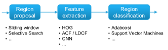
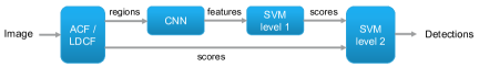
Figure 1: Detector pipelines. In (a), a typical pedestrian detection pipeline in the state of the art methods. In (b), proposed pipeline for Region based Convolutional Neural Networks (R-CNN).

Starting with the introduction of AlexNet in 2012, which won by a large margin the ImageNet Large Scale Visual Recognition Challenge [3], deep convolutional neural networks have become the dominant approach in image classification, recently achieving human-level performances [9]. The seminal work by Girschick on Regions with convolutional neural networks (R-CNN) [5] extended those results to object detection. In the R-CNN paradigm, detection is performed in two stages: first, a separate algorithm generates candidate object proposals based on e.g. region segmentation or edges; then, a CNN is run on the proposals to generate the final detection results. While for generic object detection an object agnostic method such as Selective Search [10] is necessary, for more focused tasks like pedestrian detection such proposals are under-performing compared to the state of the art [2] and by using an accurate pedestrian detector as proposal method, significant gains can be achieved. Moreover, the proposals generated by a specialized object detector have a higher probability of containing the object of interest, reducing the number of proposal regions needed: as shown by [2] in the supplemental material, only 3 proposal per images are enough to reach a recall of more than 90%. While methods for neural network compression have a long history [11], the pace of research has accelerated in response to the large networks introduced after 2012. Denil et al. demonstrated that the parameters of deep neural networks are highly redundant and can be reduced up to 20$\times$ with no appreciable loss of accuracy, giving a strong incentive to network compression.

Early approaches are based on enforcing weight sparsity, either through low-rank approximations [12] or by an opportune regularization term [13] [14], achieving a compression ratio up to 20$\times$ at the price of a 1-2% loss of accuracy. The convolutional layers of the network can be compressed either by 1-rank approximation [15], filter decomposition [16] or Tucker decomposition [17], achieving a compression rate of 5$\times$. The sparsity of convolutional layers has the added benefit of reducing the number of operations, up to 4$\times$ in the case of [14]. Other approaches replace the fully connected layers of the network (the ones contributing the most to the number of parameters) with a different kind of layer with a lower number of parameters. Examples are kernel machines [18], tensors [19], circulant matrices [20] or a cascade of diagonalized matrices [21]; convolutional layers can also be replaced by separable filters [22]. Alternatively, the network weights can be compressed by an hashing function and the hashing trick used to carry out computations directly in the compressed space. Stages with $1\times 1$ convolutions are an effective way of reducing the number of parameters in a network and they are often used in very deep networks such as the Inception architecture [23] and in Residual Networks [24]; however, when applied to smaller networks can achieve the same level of accuracy as AlexNet with 40$\times$ less parameters [25].

However, a simple strategy based on scalar quantization of the weights [26] and connection pruning [27] is surprisingly effective and with network retraining achieves a 37$\times$ compression on AlexNet with almost no loss in performance [7]. The performances of this approach are further improved by enforcing a layer-wise reconstruction penalty to the quantized weights [28].

III Proposed pipeline

The baseline CNN detector, dubbed DeepPed [8], follows from [2] in combining R-CNN with an efficient pedestrian detector used as proposal method. The Aggregated Channel Features (ACF) detector [29] has been chosen for its speed and accuracy. An improved version of ACF, known as Locally Decorrelated Channel Features (LDCF) [30], was also taken into account, but despite its higher accuracy it was discarded due to its computational complexity, which is ten times higher than ACF.

In DeepPed, an input image is analyzed by ACF and several regions are proposed as potential pedestrians, with a score associated to each region. A pre-trained AlexNet network, trained on the 1000 categories of the ImageNet challenge and publicly available, is used as starting point. The last classification layer, which is application-specific, is removed and and replaced with a Support Vector Machine (SVM). The model is then retrained by fine-tuning on the Caltech Pedestrian training dataset [31] sub-sampled by 3$\times$ as suggested by [29] and using 6-fold cross-validation to select the best performing network. The training examples are pedestrian and non-pedestrian windows chosen by ACF and selected among the highest-scoring proposals. The ACF score and the SVM score from the CNN are then further combined by stacking a second SVM trained on the validation set, which gives the final detection score.

Figure 2 shows the performance of the final DeepPed pipeline compared with other state-of-the art approaches in pedestrian detection. The details of the algorithm are discussed in [8], where each step of the pipeline is analyzed and optimized in order to increase the final detection accuracy. In the following sections, we focus on reducing the space required to store the parameters of this network.

IV Model compression

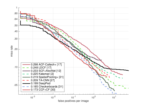
Figure 2: Comparison between the proposed DeepPed (solid black line) and other popular pedestrian detection algorithms. Note that the proposed method does not make use of multiple frame information, i.e. it does not exploit the optical flow between contiguous frames.

In order to reduce the parameter memory, two strategies inspired by [7] have been chosen to compress the network weights: scalar quantization and weight pruning. In the first case, we consider for each layer the distribution of individual weights and we quantize their values with k-means using a variable number of centroids; in the second case, we set to zero the weights with the lowest absolute value, using different values for the threshold in order to change the proportion of non-zero weights. Finally, the two approaches are combined, either by quantizing and then pruning the resulting weights, or by pruning and then quantizing the resulting distribution. As the experiments in Section V will show, the two approaches are largely independent one from the other and thus the compression factors can be composed maintaining roughly the same accuracy level.

More in detail, the following procedures have been used to compress the weights:

• Scalar quantization: each CNN layer is compressed individually. All the weight values in the layer parameters are clustered using the k-means algorithm, where the number of centroids is chosen as a function of the compression factor. Assuming that the uncompressed weights are represented each with $B$ bits, the number of centroids is:

  $$n_{centroids}=2^{\frac{B}{f_{compr}}}$$

  Henceforth, we will consider a single precision floating point representation ($B=32$) for the uncompressed weights. The maximum achievable compression rate is thus $32$ ($n_{centroids}=2$).

• Pruning: each CNN layer is compressed individually. Weights whose absolute value is smaller than a threshold are zeroed out, i.e.:

  $$w_{i,j}=\begin{cases}0,&\text{if}\ \left|w_{i,j}\right|<threshold\\ w_{i,j},&\text{otherwise}\end{cases}$$

  The threshold is set as the $p$th percentile of the weight distribution, where $p=100\cdot(1-\frac{1}{f})$ and $f$ is the compression factor; i.e. the 75th percentile is chosen for $f=4$.

• Quantization and Pruning: The combination of both quantization and pruning lets the strengths of one method compensate the shortcomings of the other. As shown in V, a higher level of compression can be achieved with respect to the single methods alone, while reaching the same level of accuracy.

Differently for quantization, the distribution of pruned connections needs to be stored, increasing the storage requirements. For example, if a binary map coding the pruned or not-pruned status of the connections is used, the fully connected layers of DeepPed would require a map of 6.8 MB. However, in a scenario in which a hardware designer can draw on an Application Specific Integrated Circuit (ASIC) or on an Field Programmable Gate Array (FPGA) all the connections between neurons individually, the pruned weights would translate in missing connections, and since power consumption increases linearly with wire capacity loads, the pruned connections would reduce power, space and storage usage.

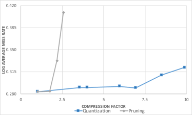
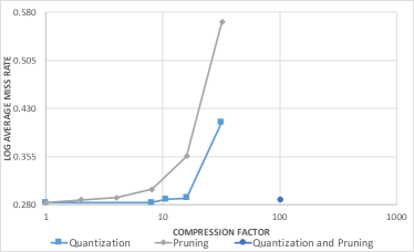
Figure 3: DeepPed results. In (a), comparison between compression by scalar quantization and by pruning in convolutional layers: the pruning method has a dramatic impact on the information content. In (b), comparison between compression by scalar quantization and by pruning in fully connected layers.

V Experimental evaluation and results

TABLE I: Final compressed model. Compression factors and sizes per layer.

Layer	CF Quantization	CF Pruning	Original size (MB)	Compressed size (MB)
Conv 1	3.56	-	0.13	0.037
Conv 2	4	-	1.17	0.293
Conv 3	4	2	3.38	0.422
Conv 4	4	2	2.53	0.319
Conv 5	4	-	1.69	0.422
Fully Connected 1	16	4	144.02	0.66
Fully Connected 2	16	4	64.02	1.35
Total	61.92		216.94	3.50

In the experiments, we tested the following approaches:

• scalar quantization alone

• weight pruning alone

• weight pruning followed by scalar quantization

Moreover, we tested the compression separately on two different set of layers:

• compressing the convolutional layers

• compressing the fully connected layers

Most of the network parameters reside in the fully connected layers, and thus the latter set is the most important; however, to reach high compression rates, both sets of layers need to be taken into account. The target size is 4 MB, a typical size for local SRAM in embedded platforms.

To assess the impact of compression on the network accuracy we resort to the evaluation metrics proposed by Dollár at al. [31] on the Caltech Pedestrian dataset. In particular, the performance of the different methods is evaluated in terms of trade-off between the compression factor (CF) and the log average miss rate (LAMR), as measured on the Caltech Pedestrian test set. The LAMR metric computes the geometric mean of the miss rate in the interval between 0.01 false detections per frame and 1 false detections per frame and can be interpreted as a smoothed estimate of the miss rate at 0.1 false detections per frame. Besides the initial fine-tuning of the DeepPed uncompressed model, the methods we tested do not require additional training, so only the test set has been used in the experiments. The original DeepPed model with ACF proposals reaches a LAMR of 28.3%.

We assess the effect of scalar quantization by measuring the accuracy of the model after compressing the fully connected (fc) layers at a factor of 8, 10.7, 16 and 32 (4, 3, 2 and 1 bit per weight) and keeping the convolutional layers unchanged. Likewise, we assess pruning by reducing the number of connections by 2, 4, 8, 16 and 32 times. The results are shown in Figure 3, with the compression factors in logarithmic scale: quantization is more efficient than pruning, and compression up to 8$\times$ can be achieved without appreciable loss of accuracy.

In the case of convolutional (conv) layers, we observe that the first layer is strongly affected by compression, while the fourth and fifth layers are more resilient. For this reason, the first layer is always compressed with 9 bits (CF=3.56) and never pruned; the remaining layers are compressed or pruned with increasingly high factors. Scalar quantization is tested at a factor of 3.56, 4, 6, 7, 8.5 and 10; pruning is tested by using the factors $\left(1,2,2,2\right)$, $\left(2,2,2,4\right)$ and $\left(2,2,4,4\right)$ for the convolutional layers from 2 to 5, resulting in overall compression factors for convolutional layers at 1.74, 2.17 and 2.57. The results are shown in Figure 3: the performances degrade much faster than in the case of fully connected layers, as expected from the fact that weight sharing in the convolutional layers already counts as a form of parameter reduction. As in the case of fully connected layers, convolutional layers are more robust to scalar quantization, achieving compression factor up to 6$\times$ with a small cost in accuracy. Pruning instead leads to a rapid degradation of performances with factors greater than 2$\times$, showing that throwing away weights with small coefficients is not desirable in convolutional layers, since the effect of these small contributions greatly influences the final accuracy.

The two methods are combined in the case of fully connected layers, where we prune $\frac{2}{3}$ of the connections and we quantize the remaining weights with 1 bit, resulting in a compression factor of 102$\times$. As Figure 3 shows, combining the two approaches actually helps both, and despite a difference of an order of magnitude in compression factor, the accuracy is comparable to scalar quantization at 10$\times$. Pruning even improves the results of quantization at 1 bit, because now the centroids need not to fit irrelevant weights. By compressing only the fully connected weights, the model already reaches a size of 10.9 MB.

TABLE II: Best performing compressed models.

Layers	Compression		Size (MB)		LAMR
	Quant.	Pruning	Original	Compr.
conv1-5	5.94$\times$		2.23	1.5	29.2% (+0.9%)
fc6-7	102$\times$		208.04	2.04	28.6% (+0.3%)
Total	61.35$\times$		216.93	3.54	28.7% (+0.4%)

We finally combine compression of convolutional and fully connected layers. Table II summarizes the performances for the best model in each scenario and for the final selected model; for the final model, Table I shows the compression factors and sizes layer by layer. The result is a model with a total size of 3.5 MB and an overall compression factor of 61.92. The final model accuracy is only slightly worse than the accuracy reachable when compressing only the fully connected layers (LAMR from $28.6\%$ to $28.7\%$), despite requiring less than one third the size of the latter. Moreover, when fully connected compression is applied together with convolutional compression, the overall accuracy increases with respect to the case when only convolutional layers are compressed (LAMR from $29.2\%$ to $28.7\%$). A possible motivation for this behavior is related to the “screening” capabilities of quantization applied on fully connected layers, acting as a filter on the noise generated in convolutional layers compression. Since 4 MB of embedded memory are viable in the 28 nm Fully Depleted Silicon On Insulator (FDSOI) STMicroelectronics fabrication process, this model enables several low-power and low-cost embedded applications.

The DeepPed architecture combined with the proposed compression scheme has been ported on an NVIDIA Jetson TK1 board and integrated with an optimized implementation of the ACF detector. The detector is capable of running at 2.4 frames per second (fps) when processing 5 proposal per frame. Moreover, by applying a tracking-by-detection algorithm such as [32] and using an average tracking length of 5 frames, the speed of the detector increases up to 10 fps, most of it spent in the CNN evaluation stage.

VI Conclusions

In this paper we present a detailed study of the effect of neural network compression in the case of a pedestrian detector and we show that a combination of simple yet effective methods allows to significanlty reduce the memory required to store the network parameters, achieving a final compression factor of 62$\times$. The behavior analysis of both convolutional and fully connected layers under scalar quantization and connection pruning shows that while the fully connected layers are the most redundant ones, high compression rates are achievable on convolutional layers with a small effect on the final accuracy. Thus, with a proper choice of compression parameters the accuracy of the system is preserved while allowing the development of embedded architectures at a small cost and low power consumption.

References

- [1] N. C. for Statistics and Analysis, “Early Estimate of Motor Vehicle Traffic Fatalities for the First Nine Months (Jan–Sep) of 2015,” National Highway Traffic Safety Administration, Washington DC, Tech. Rep., 2016.
- [2] J. Hosang, M. Omran, R. Benenson, and B. Schiele, “Taking a Deeper Look at Pedestrians,” in CVPR, Boston, MA, jan 2015.
- [3] A. Krizhevsky, I. Sutskever, and G. Hinton, “Imagenet classification with deep convolutional neural networks,” in NIPS, Lake Tahoe, NV, 2012, pp. 1–9.
- [4] K. Simonyan and A. Zisserman, “Very Deep Convolutional Networks for Large-Scale Image Recognition,” Google Research, Tech. Rep., sep 2014.
- [5] R. Girshick, J. Donahue, T. Darrell, and J. Malik, “Rich feature hierarchies for accurate object detection and semantic segmentation,” in CVPR, Columbus, OH, nov 2014.
- [6] S. Han, X. Liu, H. Mao, J. Pu, A. Pedram, M. A. Horowitz, and W. J. Dally, “EIE: Efficient Inference Engine on Compressed Deep Neural Network,” in ISCA, feb 2016.
- [7] S. Han, H. Mao, and W. J. Dally, “Deep Compression: Compressing Deep Neural Networks with Pruning, Trained Quantization and Huffman Coding,” in ICLR, San Juan, Puerto Rico, oct 2016.
- [8] D. Tomè, F. Monti, L. Baroffio, L. Bondi, M. Tagliasacchi, and S. Tubaro, “Deep convolutional neural networks for pedestrian detection,” Politecnico di Milano, Tech. Rep., oct 2015.
- [9] K. He, X. Zhang, S. Ren, and J. Sun, “Delving Deep into Rectifiers: Surpassing Human-Level Performance on ImageNet Classification,” in CVPR, Boston, MA, feb 2015.
- [10] J. R. R. Uijlings, K. E. A. Van De Sande, T. Gevers, and A. W. M. Smeulders, “Selective search for object recognition,” International Journal of Computer Vision, vol. 104, pp. 154–171, 2013.
- [11] Y. LeCun, J. S. Denker, and S. A. Solla, “Optimal Brain Damage,” in NIPS, no. 598-605, Denver, CO, 1990.
- [12] E. Denton, W. Zaremba, J. Bruna, Y. LeCun, and R. Fergus, “Exploiting Linear Structure Within Convolutional Networks for Efficient Evaluation,” in NIPS, Montreal, Canada, apr 2014.
- [13] M. D. Collins and P. Kohli, “Memory Bounded Deep Convolutional Networks,” Microsoft Research, Tech. Rep., dec 2014.
- [14] B. Liu, M. Wang, H. Foroosh, M. Tappen, and M. Penksy, “Sparse Convolutional Neural Networks,” in CVPR. Boston, MA: IEEE, jun 2015, pp. 806–814.
- [15] M. Jaderberg, A. Vedaldi, and A. Zisserman, “Speeding up Convolutional Neural Networks with Low Rank Expansions,” Arxiv, may 2014.
- [16] X. Zhang, J. Zou, K. He, and J. Sun, “Accelerating Very Deep Convolutional Networks for Classification and Detection,” Arxiv, may 2015.
- [17] Y.-D. Kim, E. Park, S. Yoo, T. Choi, L. Yang, and D. Shin, “Compression of Deep Convolutional Neural Networks for Fast and Low Power Mobile Applications,” in ICLR, San Juan, Puerto Rico, may 2016.
- [18] Z. Yang, M. Moczulski, M. Denil, N. de Freitas, A. Smola, L. Song, and Z. Wang, “Deep Fried Convnets,” in CVPR, Boston, MA, dec 2015, p. 9.
- [19] A. Novikov, D. Podoprikhin, A. Osokin, and D. Vetrov, “Tensorizing Neural Networks,” in NIPS, Motreal, Canada, sep 2015.
- [20] Y. Cheng, F. X. Yu, R. S. Feris, S. Kumar, A. Choudhary, and S.-F. Chang, “An exploration of parameter redundancy in deep networks with circulant projections,” in ICCV, Santiago, Chile, feb 2015.
- [21] M. Moczulski, M. Denil, J. Appleyard, and N. de Freitas, “ACDC: A Structured Efficient Linear Layer,” in ICLR, San Juan, Puerto Rico, may 2016.
- [22] J. Jin, A. Dundar, and E. Culurciello, “Flattened Convolutional Neural Networks for Feedforward Acceleration,” in ICLR, San Diego (CA), dec 2015.
- [23] C. Szegedy, W. Liu, Y. Jia, P. Sermanet, S. Reed, D. Anguelov, D. Erhan, V. Vanhoucke, and A. Rabinovich, “Going Deeper with Convolutions,” in CVPR, Boston, MA, jun 2015.
- [24] K. He, X. Zhang, S. Ren, and J. Sun, “Deep Residual Learning for Image Recognition,” Microsoft Research, Tech. Rep., dec 2015.
- [25] F. N. Iandola, M. W. Moskewicz, K. Ashraf, S. Han, W. J. Dally, and K. Keutzer, “SqueezeNet: AlexNet-level accuracy with 50x fewer parameters and <1MB model size,” DeepScale, Tech. Rep., feb 2016.
- [26] Y. Gong, L. Liu, M. Yang, and L. Bourdev, “Compressing Deep Convolutional Networks using Vector Quantization,” Facebook AI Research, Tech. Rep., dec 2014.
- [27] S. Han, J. Pool, J. Tran, and W. J. Dally, “Learning both Weights and Connections for Efficient Neural Networks,” in NIPS, Montreal, Canada, jun 2015.
- [28] J. Wu, C. Leng, Y. Wang, Q. Hu, and J. Cheng, “Quantized Convolutional Neural Networks for Mobile Devices,” Arxiv 2016, p. 11, dec 2016.
- [29] P. Dollar, R. Appel, S. Belongie, and P. Perona, “Fast Feature Pyramids for Object Detection,” IEEE Transactions on Pattern Analysis and Machine Intelligence, pp. 1–14, 2014.
- [30] W. Nam, P. Dollar, and J. H. Han, “Local Decorrelation for Improved Pedestrian Detection,” in NIPS, Montreal, Canada, 2014, pp. 1–9.
- [31] P. Dollár, C. Wojek, B. Schiele, and P. Perona, “Pedestrian detection: an evaluation of the state of the art,” Pattern Analysis and Machine Intelligence, vol. 34, no. 4, pp. 743–61, 2012.
- [32] M. D. Breitenstein, F. Reichlin, B. Leibe, E. Koller-Meier, and L. Van Gool, “Online Multiperson Tracking-by-Detection from a Single, Uncalibrated Camera.” IEEE transactions on pattern analysis and machine intelligence, vol. 33, no. 9, pp. 1820–33, sep 2011.