Monte-Carlo modelling of multi-object adaptive optics performance on the European Extremely Large Telescope

Abstract

The performance of a wide-field adaptive optics system depends on input design parameters. Here we investigate the performance of a multi-object adaptive optics system design for the European Extremely Large Telescope, using an end-to-end Monte-Carlo adaptive optics simulation tool, DASP, with relevance for proposed instruments such as MOSAIC. We consider parameters such as the number of laser guide stars, sodium layer depth, wavefront sensor pixel scale, actuator pitch and natural guide star availability. We provide potential areas where costs savings can be made, and investigate trade-offs between performance and cost, and provide solutions that would enable such an instrument to be built with currently available technology. Our key recommendations include a trade-off for laser guide star wavefront sensor pixel scale of about 0.7 arcseconds per pixel, and a field of view of at least 7 arcseconds, that EMCCD technology should be used for natural guide star wavefront sensors even if reduced frame rate is necessary, and that sky coverage can be improved by a slight reduction in natural guide star sub-aperture count without significantly affecting tomographic performance. We find that adaptive optics correction can be maintained across a wide field of view, up to 7 arcminutes in diameter. We also recommend the use of at least 4 laser guide stars, and include ground-layer and multi-object adaptive optics performance estimates.

1 Introduction

The next generation of ground based astronomical telescopes will be the Extremely Large Telescopes (ELTs) (Spyromilio et al., 2008; Nelson & Sanders, 2008; Johns, 2008), which are due to see first light within the next decade. All of these telescopes rely on adaptive optics (AO) systems (Babcock, 1953) to provide compensation for the degrading effects of atmospheric turbulence, thus allowing the scientific goals of these facilities to be met. Extensive simulation of AO systems is required during the instrument design phases, so that predicted performance estimates can be made and design trade-offs explored and AO designs optimised.

High fidelity modelling of the performance of AO and telescope systems can be implemented using Monte-Carlo simulation, which involves playing a time sequence of input atmospheric perturbations through the AO system and telescope models. For ELT-scale instruments, these simulations are computationally expensive. Here, we report on an exploration of the parameter space related to a multi-object AO (MOAO) system design study for the 39 m European ELT (E-ELT). We use the Durham AO simulation platform (DASP) (Basden et al., 2007; Basden & Myers, 2012) to perform this modelling. Our models are based on a system with both laser guide stars (LGSs) and natural guide stars (NGSs) (the number of which we explore), and we use a high resolution atmospheric model (as used in previous studies, e.g.  Basden, 2015b) which is stratified into 35 discrete layers of turbulence. Our results have relevance for proposed and future MOAO instruments such as MOSAIC, and also more generally for other wide-field AO systems.

Within this study, we investigate factors such as the number of LGSs, the elongation of LGSs as seen by the wavefront sensors (WFSs) (due to the extent of the mesosphere sodium layer depth), the number, position and magnitude of NGSs within the field of view, deformable mirror (DM) requirements, detector requirements, WFS sensitivity and field of view and the effect of turbulence strength. We explore AO performance across the field of view, and our default results are presented on-axis, which we show to be pessimistic compared to most of the rest of the field of view. We also consider the performance improvements achievable by operating the LGS and NGS WFSs at different frame rates, and consider the use of currently available commercial cameras as wavefront sensors.

The results that we present can be used to aid design decisions for ELT instrumentation, and also to provide a benchmark for simulation comparison. These results are complementary to those from other modelling tools for ELT MOAO instrumentation (which for a single on-axis channel can be viewed as laser tomographic AO (LTAO)), for example Le Louarn et al. (2012); Arcidiacono et al. (2014).

In §2 we present the key parameters of our simulations, and details of the parameter space that is explored, along with key algorithms. In §3 we present our resulting estimates of AO system performance, and we conclude in §4.

2 ELT-scale MOAO system modelling

We base our modelling on DASP, which has been cross checked and verified against other AO simulation codes, and which has a long history of AO system modelling. In a previous study (Basden et al., 2014), we explored many different NGS asterisms available within a cosmological field (which by definition are relatively free of suitable bright guide stars), and the effect that these have on AO performance. Here, we base this study on the same set of NGSs, as shown in Fig. 1. Unless otherwise stated, we use asterism 0 as the default case, as this provides a close-to-median performance. Conversion from guide star magnitude to detected WFS flux level is given by Basden et al. (2014)

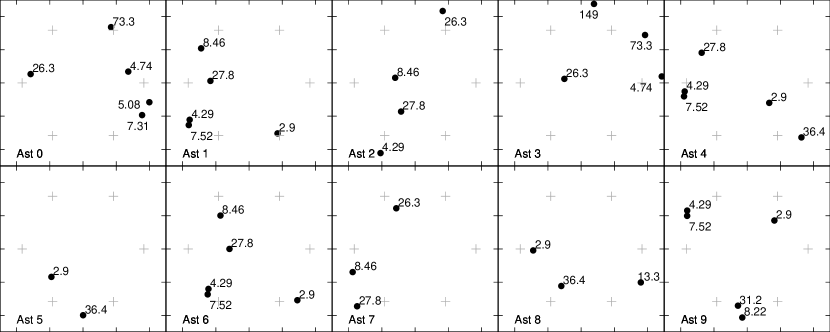
Figure 1: A figure showing the NGS asterisms, and LGS positions, that are used throughout this study. The numbers next to the guide stars represent flux in photons per sub-aperture per frame at 250 Hz. The LGS positions are given by +. Asterism number is denoted by “Ast”. The total field of view across each asterism is 10 arcminutes, and the axis tick marks are 2 arcminutes apart.

The key AO performance metric that we present here is ensquared energy within a 150 mas box diameter at H-band (1650 nm wavelength). The reason for this is that for a wide-field MOAO system with limited guide star numbers (both NGS and LGS), Strehl ratio is typically low, and ensquared energy is therefore more sensitive to changes in AO performance as parameter space is explored. Additionally, MOAO instruments are typically coupled to spectrographs, and of relevance here is how much light (energy) can be fed into an optical fibre. However, we also consider other performance metrics, and performance at other wavelengths. We ensure that the science point spread functions (PSFs) are well averaged, and typically integrate for 20 s of telescope time (5,000 iterations). The uncertainties in our results due to Monte-Carlo randomness are below 1%, which we have verified using a suite of separate Monte-Carlo instantiations.

We ignore the tip-tilt signal from the LGSs (since this is generally not known), and we use the NGSs for full high order correction, in addition to tip-tilt correction. Where NGS flux is particularly low, we investigate reducing the frame rate of these particular WFSs (to increase the flux). When doing this, wavefront reconstruction is performed using the newest available measurement, at the rate of the fastest wavefront sensor, i.e. a zero-order hold for the slower WFSs. We do not investigate more complicated algorithms.

The E-ELT design has a “deformable secondary” DM (actually the fourth mirror in the optical train, M4). Our simulations therefore have a 2-DM design, using this M4 DM to perform a global ground layer correction, and then individual MOAO DMs to compensate along a specific line of sight. We assume that M4 is optically conjugated to the ground layer, though in the E-ELT design it is actually conjugated at about 625 m. However, a previous study has shown that this has a negligible effect on AO performance (Basden, 2015b).

2.1 Details of the simulation model

The simulations presented here use a standard European Southern Observatory (ESO) turbulence profile for the E-ELT site (Sarazin et al., 2013), containing 35 turbulent layers extending up to about 20 km. The default outer scale is 25 m with a 13.5 cm Fried’s parameter (at zenith). Five variations of this profile are studied, with the median seeing case, and one case for each quartile. Unless stated otherwise, we assume the median profile, and we observe at 30^∘ from zenith. We assume an AO system update rate of 250 Hz, which is fairly typical for MOAO systems (Lardière et al., 2014; Gendron et al., 2011; Basden et al., 2016) and has been used in previous studies of ELT MOAO systems (Basden, 2014). For wide-field AO systems, AO latency does not tend to dominate the error budget, and therefore we do not present any investigations of AO frame rate here, other than reductions in the speed of faint NGSs as mentioned previously.

We assume a primary mirror diameter (largest optical diameter) of 38.55 m, and the M4 DM has $75\times 75$ actuators in a square grid by default. We also compare performance with a hexagonal actuator pattern. We assume a telescope central obscuration diameter of 11 m, and our models include the hexagonal edge pattern based on a primary mirror design created from 798 segmented hexagonal mirrors, matching the E-ELT. The telescope pupil function is modelled as direction dependent, with vignetting by the central obscuration changing depending on line of sight. We also include telescope support structures (spiders) in this pupil function, following models used by Basden (2015b).

2.1.1 Wavefront sensors

In our default case, the wavefront sensors all have $74\times 74$ sub-apertures. We also consider AO performance when the number of NGS WFS sub-apertures are reduced (to increase individual sub-aperture flux). We use up to 5 NGSs (at positions given by Fig. 1), and up to 6 LGSs (6 for the default case) equally spaced around a circular asterism which has a default diameter of 7.3 arcmin. The LGSs are side-launched from four launch locations, spread equally around the telescope, 22 m from the central axis. Our default simulation uses a sodium layer with a Gaussian profile and a full-width at half-maximum (FWHM) depth of 10 km, centred at 90 km above the ground (with focal anisoplanatism). We assume that the LGS PSFs have a 1 arcsecond FWHM across the spot profile, due to a combination of atmospheric broadening and a finite width laser plume. Combined with our default LGS pixel scale and sub-aperture size, this results in a small amount of spot truncation with sub-apertures furthest from the laser launch aperture having flux reduced by about 2.5% due to truncation. The default LGS flux is 5000 photons per sub-aperture per frame (approximately 6 million photons m^-2 s^-1 on-sky with a 90% telescope throughput and an 85% WFS throughput), and we investigate other signal levels. This flux level is chosen based on measurements of sodium layer return flux by the ESO Wendelstein LGS unit (Bonaccini Calia, 2016) which returns between 5–21 million photons m^-2 s^-1.

Sub-apertures typically have $16\times 16$ pixels, unless otherwise stated. For the LGS WFSs, this helps to reduce the effects of spot truncation. For the NGS WFSs, such a large field of view is not strictly necessary, but is used for simplicity. We do however investigate smaller sub-apertures. We include readout noise, with a default value of 0.1 electrons per pixel, corresponding to electron multiplying CCD (EMCCD) technology, and investigate performance with up to 3 electrons readout noise, corresponding to equivalent levels experienced by scientific CMOS (sCMOS) technology detectors due to the non-Gaussian distribution of readout noise (Basden, 2015a). Photon shot noise is also included. We apply a threshold to the sub-apertures before slope calculation which has a default value of three times the readout noise.

Our default wavefront sensor pixels scale is 0.7 arcseconds per pixel for the LGS WFSs, and 0.25 arcseconds per pixel for the NGS WFSs.

Since instrumental and telescope optical throughputs, and precise detector quantum efficiencies are not well known, we also investigate AO performance when NGS flux is increased and reduced, to provide an estimation for sensitivity to changes in detected flux.

2.1.2 Wavefront reconstruction

We perform tomographic wavefront reconstruction using a virtual DM approach. First, wavefront sensor signals are reconstructed at several discrete heights to give an estimate of the wavefront phase at these locations. Projection along a given line of sight then provides the signal which is sent to the individual MOAO DMs, which are conjugated to the telesecope pupil. We find that using 12 such virtual DMs gives good performance, with little gained by using an increased number (and using fewer leads to reduced performance). The virtual DMs are conjugated close to dominant atmospheric layers, and the position of these is modified when using different atmospheric profiles.

The pitch of phase reconstruction is dependent on layer strength rather than constant (Gavel et al., 2003), to help reduce computational load, though is fixed at the LGS sub-aperture pitch for the ground conjugate DM. We find that slightly improved performance can be obtained using an increased number of phase reconstruction points for non-ground conjugate DMs, though do not present this here. Wavefront reconstruction is based on a minimum mean square error (MMSE) algorithm (Ellerbroek et al., 2003). We approximate wavefront phase covariance using a Laplacian regularisation, and noise covariance is approximated to a single value for each wavefront sensor, dependent on flux and readout noise. Although this is slightly sub-optimal, it allows us to simplify our modelling.

2.1.3 Deformable mirrors

The DMs are modelled using a cubic spline interpolation function, which uses given actuator heights and positions to compute a surface map of the DM. The MOAO DMs have $64\times 64$ sub-apertures by default, though we also investigate lower actuator counts, to match a range of commercially available DMs. A previous study has investigated required stroke and DM imperfections (Basden, 2014).

3 Wide field of view MOAO performance estimation for the E-ELT

When designing an AO system, maximum performance is always desirable. However, budget limitations usually mean that design trade-offs must be made. Here, we present results from several trade-off studies that will allow ELT MOAO performance to be optimised within a given budget.

Fig. 2 shows predicted AO performance (ensquared energy within a 150 mas box size) across the 10 arcminute field of view for our default simulation case, at multiple wavelength bands. It can be seen that within the LGS asterism diameter, AO correction is relatively uniform, but that performance drops faster outside.

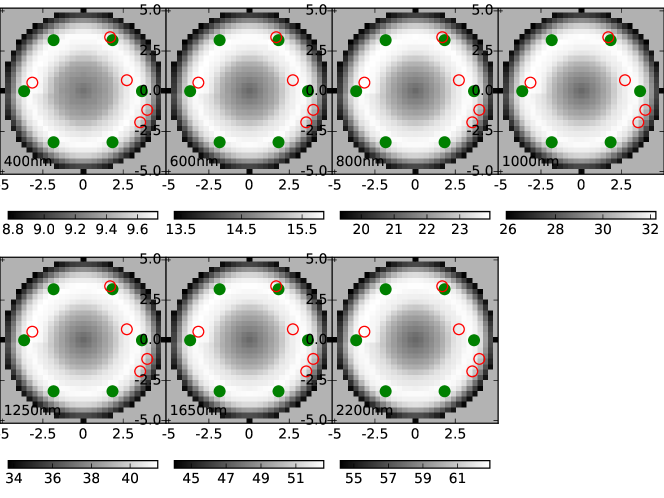
Figure 2: A figure showing predicted ensquared energy in a 150 mas box across a 10 arcminute field of view at the wavelengths given on the sub-figures. The LGS positions are shown by filled green circles, and the NGS positions by unfilled red circles.

3.1 The effect of LGS WFS pixel scale on AO performance

The sensitivity of a WFS is determined in part by its pixel scale. For elongated LGS spots, there is a trade-off between the number of detector pixels per sub-aperture (each of which introduces noise), the spot size (with elongation determined by off-axis distance and sodium layer profile), the expected range of spot motion, and the number of pixels over which flux is distributed. Fig. 3 shows predicted on-axis AO performance as a function of sodium layer depth for different pixel scales (resulting in different elongation of Shack-Hartmann spots). In this case, each sub-aperture has $16\times 16$ pixels, and receives a mean flux of 5000 photons per frame. It can be seen here that for larger sodium layer depths, it is favourable to have larger pixel scales. We have therefore selected 0.7 arcseconds per pixel as the default for this study, since performance remains good up to depths of 30 km which is a likely upper limit (Pfrommer & Hickson, 2014). We note that a smaller pixel scale would lead to an improvement of a few percent in ensquared energy when sodium layer depth is small. However, this gain quickly drops off as the depth increases, and 0.7 arcseconds per pixel is a good compromise.

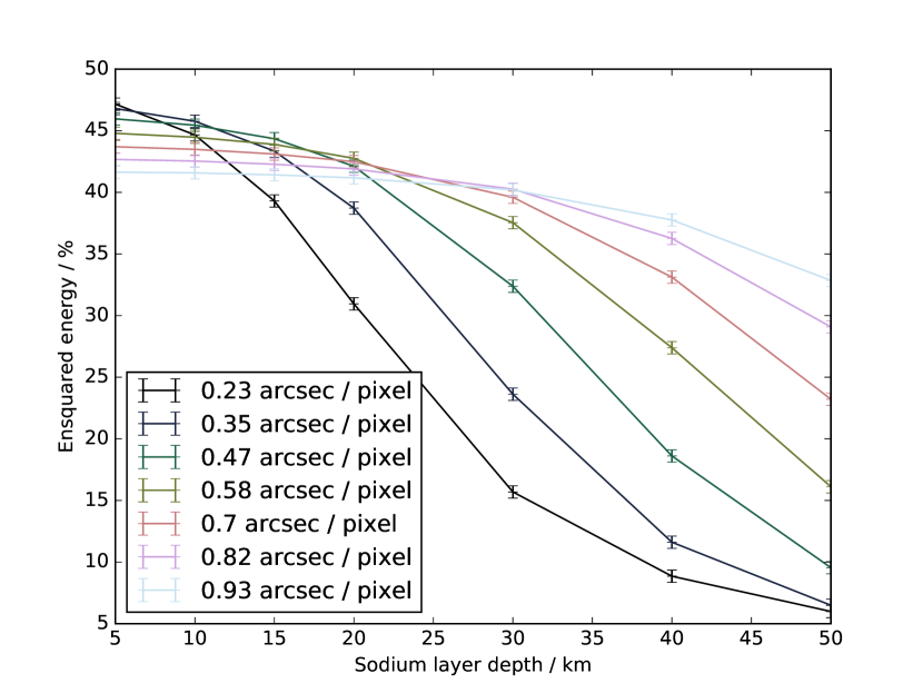
Figure 3: A figure showing on-axis AO performance (H-band ensquared energy within a 150 mas box) as a function of sodium layer depth (full width half maximum) for different pixel scales as given by the legend.

We also investigate the effect of a reduction in number of pixels per LGS sub-aperture. This is of interest in instrument designs because a requirement for fewer pixels equates to smaller detectors, increasing the likelihood of commercial availability. Additionally, fewer pixels have reduced readout noise, increasing performance, but also contribute to greater truncation of elongated LGS spots. We find (Fig. 4(a)) that is only slightly affected by sub-aperture size, until LGS spots become more severely truncated (Fig. 4(b)).

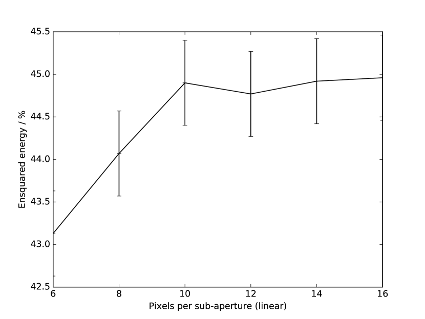
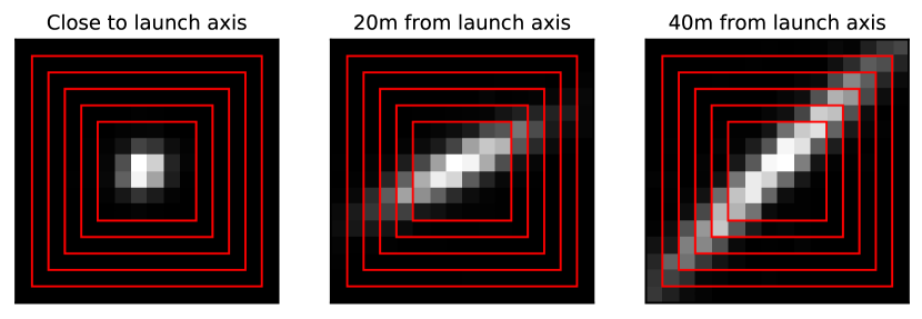
Figure 4: (a) A figure showing AO performance (H-band ensquared energy in 150 mas) as a function of linear sub-aperture size in pixels. The pixel scale is kept constant at 0.7 arcsec per pixel. (b) Showing the LGS truncation for different sub-apertures at increasing distances from the LGS launch axis. The boxes show sub-aperture sizes from $6\times 6$ to $16\times 16$ pixels, and the sodium layer depth FWHM is 10 km

3.2 Exploration of LGS number

We have previously explored MOAO performance with a number of different NGS asterisms (Basden et al., 2014). Here, for each of these asterisms, we investigate performance as a function of number of LGSs used, as shown in Fig. 5. It can be seen that the rate of drop in performance is dependent on the NGS asterism, and that in particular, asterism 5 gives poorer performance. We note that this particular asterism contains only 2 stars, and that one of these is very faint (2.9 photons per pixel per frame at 250 Hz).

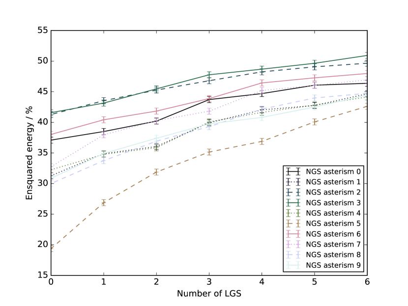
Figure 5: A figure showing on-axis AO performance (H-band ensquared energy within a 150 mas box) for different numbers of LGSs, and different NGS asterisms.

We note that this result does not point to a conclusive LGS requirement. Performance is seen to increase as guide star number increases, and for particular NGS asterisms can drop off sharply when few LGSs are used. It is encouraging that good performance is seen with 4 LGSs, since this is the current baseline number that will be provided by ESO at the E-ELT. Whilst maximum performance for the best asterisms drops from 52% to 48% as LGS number is decreased from 6 to 4, performance with the worst performing asterism drops from 42% to 37%.

We also note that when number of LGS is reduced, it would be possible to compensate the performance loss by increasing the number of NGSs. However, this is not something that we investigate, partly due to the reduction in sky-coverage that would ensue, and because of the increase in system complexity with greater numbers of natural guide star acquisition systems.

3.3 Reduction in frame rate and sub-aperture count of faint NGSs

Given that some of the NGSs within our chosen asterisms are extremely faint, there are two obvious ways in which flux can be increased. Either, sub-aperture count can be reduced (so spreading available flux between fewer sub-apertures), or the WFS frame rate can be reduced (allowing longer integration times). Having a variable sub-aperture count in an AO system is not always simple if Shack-Hartmann systems are used: an optical realignment is required, and mechanisms are required to change the lenslet arrays. This is not an attractive prospect for an ELT-scale MOAO system, however one possibility may be to have a pre-defined number of high and low order wavefront sensors present, which can then be selected depending on target availability. Alternatively, a Pyramid wavefront sensor (Ragazzoni, 1996) can be used, which provides the ability to re-bin wavefront sensor images on-the-fly. Here, we do not consider the use of Pyramid sensors as the relative merits of Shack-Hartmann and Pyramid systems have been explored elsewhere, and are not part of the baseline design for the current E-ELT MOAO instrument concept. Additionally, pyramid sensors are non-linear, which for a partially open-loop instrument such as the MOAO instruments simulated here, introduces significant additional complexity. Techniques to combine pyramid and Shack-Hartmann wavefront sensor signals in a tomographic AO system are also not well studied. However we note that this would potentially be another way to improve performance. To simplify our investigation, we consider the case in which the sub-aperture count of all NGS WFSs is reduced, and expected performance is shown in Fig. 6. It can be seen that a factor of two reduction in sub-aperture count (across the pupil) can lead to slight performance improvement for some asterisms under consideration, but that further reductions lead to worse performance, i.e. NGS information is required for tomographic wavefront reconstruction. However, we suggest that in cases where sky coverage is important, NGS WFS sub-aperture count could be reduced, increasing coverage, but leading to slightly lower performance overall. We also consider the case where slope measurements from a high order ($74\times 74$) sensor are averaged to give a global tip-tilt measurement (i.e. using the NGS for tip-tilt only, without requiring optical modifications). However, this yields a more significant drop in performance (with H-band ensquared energy within 150 mas dropping to about 30%). Therefore, we do not consider this option further here.

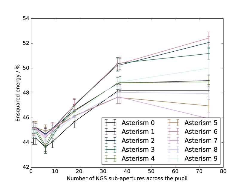
Figure 6: A figure showing on-axis AO performance (H-band ensquared energy within a 150 mas box) as a function of number of NGS sub-apertures, for the different NGS asterisms under consideration.

A reduction in faint NGS WFS frame rate can also be used to increase detected NGS flux, and one which can be performed entirely by the software controlling the AO system (i.e. no changes to the optical or mechanical design are required). To investigate this, we take a pragmatic approach: we assume that the LGS WFSs and bright NGS WFSs will operate at the baseline frame rate of 250 Hz. We then reduce the frame rate of fainter NGS WFSs in steps of size equal to the time period of the LGS WFSs (4 ms), until the detected flux for these WFSs reaches some set level. For example, if we specify a minimum flux of 20 photons per sub-aperture per frame, then a WFS that measures 15 photons at 250 Hz would be reduced to 125 Hz (delivering 30 photons) and a WFS that measures 7 photons at 250 Hz would be reduced to 83 Hz (3 time steps), delivering 21 photons. Fig. 7 shows predicted on-axis AO performance for this investigation. It is clear that this approach can significantly increase AO performance when sources are faint. In general, we find that a minimum flux of about 10 detected photons per sub-aperture offers best performance for the asterisms studied.

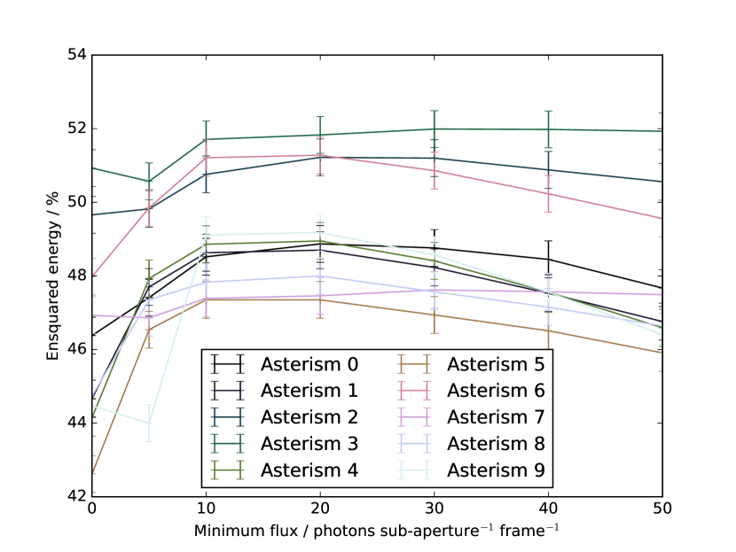
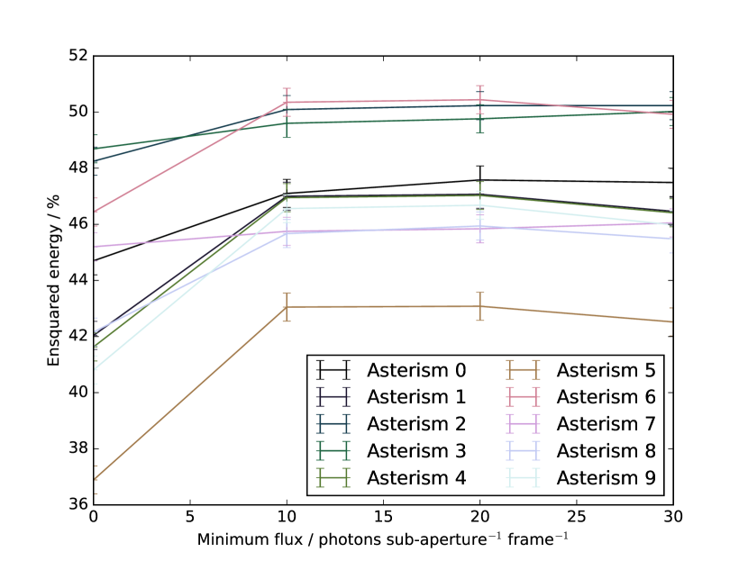
Figure 7: A figure showing on-axis AO performance (H-band ensquared energy within a 150 mas box) as NGS frame rate is reduced so that a given minimum flux is recorded (given by the x-axis), for (a) 6 LGS, and (b) 4 LGS.

3.4 Investigation of commercial WFS detector configurations

In order to reduce risk associated with development of a MOAO system, we here consider the use of a commercially available detector for the NGS WFSs, a $1024\times 1024$ EMCCD. We use camera specifications of an Andor Technologies iXon Ultra 888 (Technologies, 2016) which has a maximum frame rate (full frame) of 26 Hz. We also note than an Imperx Puma camera (Imperx, 2016) would also meet these specifications. We assume 0.1 electrons readout noise, and the modes of operation that we consider are given in table 1. We have focused on this detector for several reasons:

1. It has enough pixels to provide a reasonable sub-aperture size, to avoid centroid gain variations due to changes in seeing.

2. It has low readout noise, essential for increasing sky coverage.

3. It has a frame rate that (as we show) is sufficient to not significantly affect AO performance.

For the NGS WFSs, we also consider the use of the proposed (not yet available) ESO LGSD dectector with a $1760\times 1680$ pixels, and a maximum frame rate of over 250 Hz (Downing et al., 2014). This detector is specified with a readout noise of 3 electrons.

Window size	AFR (MFR)	Pixels per	Number of LGS
	/ Hz	sub-aperture	integrations per NGS
			frame
$962\times 962$	27.8 (30)	$13\times 13$	9
$888\times 888$	35.7 (36)	$12\times 12$	7
$740\times 740$	50 (52)	$10\times 10$	5
$592\times 592$	62.5 (75)	$8\times 8$	4
$444\times 444$	83.3 (110)	$6\times 6$	3

Table 1: A table showing possible modes of operation for the NGS using a $1024\times 1024$ pixel EMCCD. The maximum frame rate (MFR) of the camera for each mode of operation is given, though we reduce this for each case to ensure a whole number of 250 Hz LGS integrations fit in each NGS frame period, given by the actual frame rate (AFR).

For the LGS WFSs we assume $16\times 16$ pixels per sub-aperture and 3 electrons readout noise. We note that there are two distinct detector possibilities that can meet this specification, though neither is yet commercially available in a suitable camera. The first is the ESO LGSD (Downing et al., 2014) (manufactured by E2V), while the second is the Fairchild Imaging LTN4625A sCMOS detector (Systems, 2014).

For the NGS WFSs, we investigate the trade-off between maximum frame rate, and number of pixels per sub-aperture in Fig. 8. Here we can see that better performance is achieved using a higher frame rate, and hence fewer pixels per sub-aperture. For comparison, the case using the LGSD detector for the NGS WFSs is also shown, and it is evident that performance is far worse, primarily due to the higher readout noise. We therefore recommend the use of lower readout noise detectors for the NGS WFSs even if these are required to run at lower frame rates.

When the detector with 0.1 electrons readout noise is used, frame rate must be reduced (Table 1) due to camera readout modes. Fig. 8 displays two sets of information for clarity. Firstly, we reduce the camera frame rate (increase the exposure time), but do not add any additional readout delay (signified by “no readout delay” in the legend). We note that is unphysical with this detector. We therefore also reduce the frame rate, and increase the readout time, to give actual achieved performance (signified by “Readout delay” in the legend). It is therefore evident that this additional delay begins to have significant impact, and that therefore, smaller sub-apertures (with increased frame rate) are favoured. For comparison, we also show performance using NGS asterism 5, demonstrating that good performance can be achieved even in the challenging case of the sparsest identified NGS asterism.

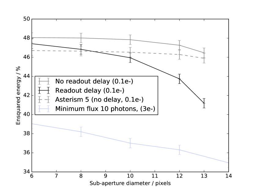
Figure 8: A figure showing AO performance (on-axis H-band ensquared energy in a 150 mas box) for the different NGS WFS camera options described in the text and legend. Asterism 0 is used unless otherwise stated. For the 0.1e- readout noise case, frame rate is reduced as per table 1, while a frame rate of 250 Hz is assumed for the 3e- readout noise case, reduced for faint guide stars such that at least 10 photons per sub-aperture per frame are delivered.

We note that we do not include the impact of telescope vibrations within these results. Therefore the results given at lower frame rates are likely to be more optimistic, since lower frame rates will suffer more from uncorrected vibrations, even when vibration mitigation techniques, such as linear-quadratic-gaussian (LQG) control, are used (Sivo et al., 2014). Higher order vibrational modes can be compensated using LGS measurements. It is only the lowest order modes (tip-tilt), with correspondingly lower frequencies, which would require NGS signals for correction.

Our recommendation for wavefront sensor detector technology is therefore to use low readout noise EMCCD detectors for the NGS WFSs, which can be operated at a lower frame rate, and higher readout noise complimentary metal-oxide semiconductor (CMOS) detectors for the LGSs, where larger detector area is important to prevent performance degradation due to spot truncation, and where incident flux can be higher such that the increased readout noise has less of an impact. The increased readout rates of large CMOS devices (compared with equivalent sized EMCCDs) is also advantageous for the LGSs.

3.5 NGS flux investigation

Since instrumental and telescope optical throughputs are not known, we investigate performance as a function of NGS flux, i.e. we apply a global scaling to the flux provided by a given NGS asterism. Fig. 9 shows these results for one NGS asterism (asterism 0), and these can be compared with Basden et al. (2014). This figure also demonstrates how AO performance can be improved by reducing the WFS frame rate used with low-flux NGSs. Here, we can see that in the case of the NGS asterism 0 studied here, by reducing NGS WFS frame rates so that each sub-aperture contains at least 10 photons per frame, an improvement in performance can be seen compared with when all wavefront sensors operate at the same frame rate. For comparison, when no NGSs are used (and the LGS tip-tilt signal is assumed valid), ensquared energy within a 150 mas box is found to be about 24%.

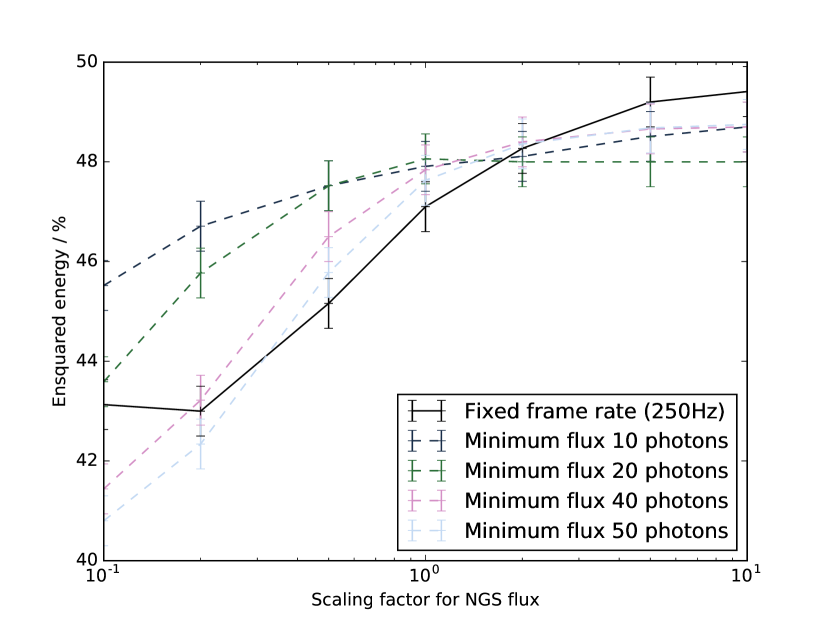
Figure 9: A figure showing AO performance (H-band ensquared energy within 150 mas) as a function of globally scaled NGS flux. Shown are plots for all WFSs having the same frame rate (250 Hz), and where NGS WFSs have reduced frame rate such that a minimum flux level is recorded, as given in the legend (in photons per sub-aperture per frame).

3.6 LGS flux investigation

In contrary to NGS flux which is known, LGS flux will vary depending on conditions within the sodium layer. We therefore explore AO performance as a function of LGS return flux level. We consider several different detector scenarios, each with different readout noise levels. First, we consider the case where the LGS and NGS WFS cameras have identical readout noise (from 0.1 to 3 electrons). We then also consider the case where the NGS WFS readout noise is fixed at 0.1 electrons (since we know that such a detector exists, as described in §3.4), while LGS readout noise varies. The range of LGS flux used is given from measured on-sky flux return (Bonaccini Calia, 2015).

Fig. 10 shows the results, and it can be seen that when the NGS WFS readout noise is low, the expected LGS flux is sufficient to maintain good AO performance. However, when both LGS and NGS WFS readout noise increase AO performance drops. Therefore, if instrumental trade-offs must be made related to detector readout noise, it would be advantageous to ensure that low readout noise for the NGS WFS is prioritised. LGS WFS readout noise level is not critical with the expected LGS flux return at these frame rates.

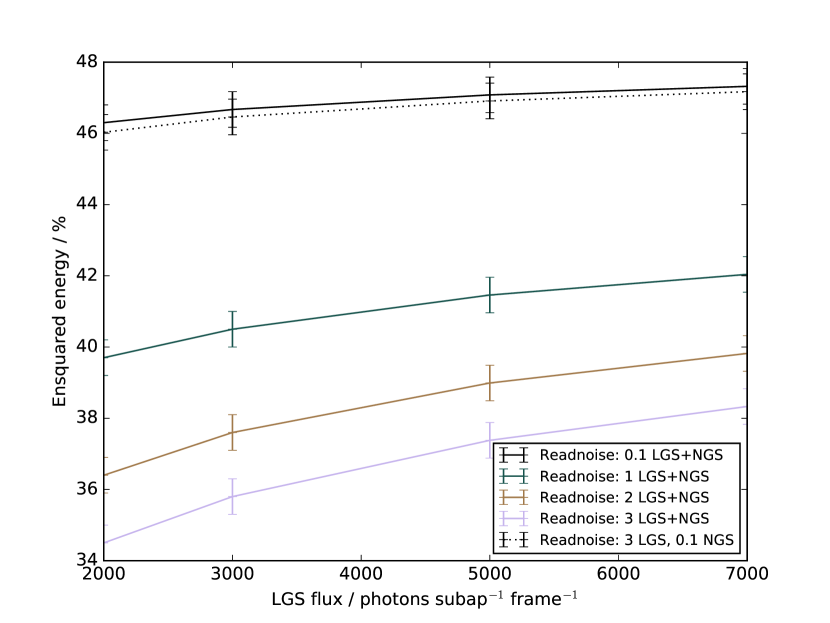
Figure 10: A figure showing AO performance (H-band ensquared energy within 150 mas) as a function of LGS flux (in photons per sub-aperture per frame), for different detector readout noise levels, as given in the legend. For solid curves, the LGS and NGS detectors have the same readout noise (given in the legend). For the dashed curve, the NGS has a readout noise of 0.1 electrons, while the LGS readout noise is given in the legend.

3.7 LGS asterism diameter

Although the performance of LTAO and MOAO as a function of LGS asterism diameter has been well studied elsewhere (Le Louarn et al., 2012; Basden et al., 2013), we include here such a study, to provide a reference, and for comparisons with other results. Fig. 11 provides this information for both H-band Strehl ratio and ensquared energy (with a 150 mas box size).

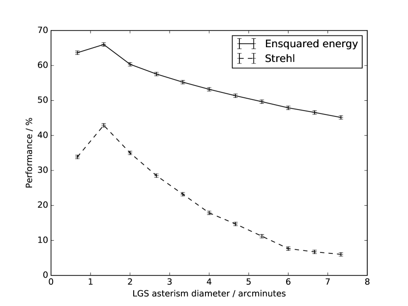
Figure 11: A figure showing AO performance at H-band as a function of LGS asterism diameter. Ensquared energy is within a 150 mas box size.

3.8 Guide star asterism rotation

When operating multiple LGS AO systems, there are two possibilities for LGS tracking: either they can track the telescope pupil, or track the sky rotation during observations. In the former case, relative alignment between the LGS and un-de-rotated components (such as M4) will remain constant, while relative alignment between the LGS and NGS WFSs will change. Therefore, continual update of the tomographic reconstruction matrix will be necessary to account for the change in relative WFS alignment. The required frequency of this update is determined by the tolerance of AO performance to mis-rotation.

In the latter case, relative alignment between M4 and the WFSs will change, and it is necessary to be able to steer the LGSs (to maintain tracking). The relative WFS alignments will also change with flexure and rotation of lenslet arrays with respect to other guide stars.

The impact of sub-aperture rotation has been studied previously (Basden et al., 2013). Here, we consider only the effect of LGS motion (tracking the sky) resulting in a change in tomography, i.e. in portion of the atmosphere through which the LGS propagates. These simulations do not include the effect of rotation of wavefront sensors with respect to others. Fig. 12 shows AO performance as a function of rotation angle between the on-sky guide star positions, and provides information on how frequently a wavefront reconstruction matrix must be updated to maintain performance during AO operation. Here, we rotate the on-sky position of either the LGSs or the NGSs. Sub-aperture alignment remains constant, i.e. aligned with DM actuators. This figure therefore shows how performance changes as the guide stars sample different parts of the turbulent volume than the tomographic reconstruction expects. We note that the drop in performance is relatively small. This is to be expected because ground layer sampling remains unaffected (it is sampled regardless of where the guide stars point), and the ground layer encompasses a significant amount of turbulent strength. We see that performance is maintained for differential rotations of up to about one degree. Therefore, update of the tomographic control matrix is necessary whenever the relative sky-pupil rotation becomes larger than one degree. We note that this figure does not include any differential rotation of the WFS sub-aperture alignment, or between the DM actuator grids and the sub-aperture grids. These effects could have a large impact in practice, and so in the case where the wavefront sensor alignment is not maintained (by optical derotation), further investigation would be necessary.

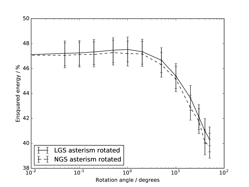
Figure 12: A figure showing AO performance (H-band ensquared energy within a 150 mas box) as a function of differential rotation between DMs and on-sky guide star position.

3.9 DM actuator count

DMs are key components within an AO system, and for a MOAO system which requires one DM per channel, can introduce a significant cost to the overall design. Higher order DMs are generally more expensive, and therefore it may be attractive to reduce system cost by reducing the number of DM actuators. We have therefore investigated AO performance when using MOAO DMs of different orders, as shown in table 2, for 3 currently available DM sizes. We see that reducing DM order leads to a drop in AO performance. However, individual instrumental science requirements may mean that performance goals can still be met with a lower performance, and so using lower order DMs should not be ruled out simply because performance is reduced. We note that these results are similar to those reported by Basden et al. (2013).

M4 actuator geometry	MOAO	Strehl	EE
	actuator count
Square $75\times 75$	$64\times 64$	6.77	46.9
Square $75\times 75$	$32\times 32$	4.38	41.0
Square $75\times 75$	$17\times 17$	2.88	35.7
Hexagonal $75\times 65$	$64\times 64$	6.31	46.0

Table 2: A table showing H-band on-axis AO performance for different DM configurations (EE is ensquared energy is within a 150 mas box size).

We also consider the use of a hexagonal actuator pattern for M4, (the global ground layer correction), with the DM having $75\times 65$ actuators. As expected, this only has a small impact on performance (given in the table), and so, for generality, we have used a square actuator pattern throughout this paper.

3.10 Sensitivity to atmospheric turbulence profiles

We have been using median seeing from the standard ESO 35-layer atmospheric profile (Sarazin et al., 2013) for these simulations. However, under different seeing conditions, AO performance can be significantly different. Table 3 shows how AO performance is expected to vary using the defined 4 quartile profiles. Additionally, AO performance when using an alternative 31-layer atmospheric profile (which is defined in ESO internal document ESO-191766v7) is also given. We see here that under poor atmospheric conditions, AO performance is significantly worse. Therefore when designing an AO instrument to meet specific science requirements, it is important to specify observing condition, i.e. should science requirements always be achievable, or only some fraction of the time.

Profile	Strehl	Ensquared energy	GLAO ensquared
			energy
Quartile 1	17.3	61.2	42.7
Quartile 2	8.4	48.3	29.9
Median	5.2	46.9	24.0
Quartile 3	3.0	36.9	19.5
Quartile 4	0.7	22.1	5.9
31-layer	5.6	47.4	12.6

Table 3: A table showing H-band AO performance under different atmospheric conditions. Ensquared energy is within a 150 mas box.

3.11 GLAO performance

An MOAO system is able to perform tomographic ground layer AO (GLAO) correction for free, using either a common DM (e.g. E-ELT M4), or the individual MOAO DMs (since these are usually ground conjugated).

We therefore investigate GLAO performance as a function of LGS asterism diameter, and number of LGSs. As seen in Fig. 13, performance is fairly insensitive to these changes, since all configurations are able to identify the ground layer. However, we note that the correction quality is significantly degraded from that achieved using MOAO, i.e. GLAO ensquared energy is only about half of the MOAO energy for the given atmospheric profile. Here, we have assumed that the GLAO DM is conjugated at zero. However, as mentioned previously, the E-ELT M4 DM is expected to be conjugated at about 625 m. A previous study (Basden, 2015b) has shown that this difference is expected to have little impact on performance.

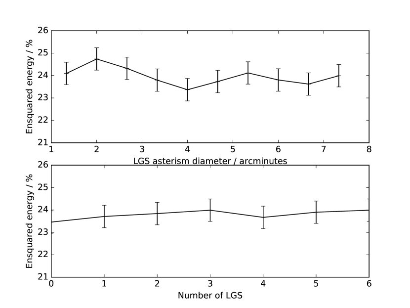
Figure 13: A figure showing GLAO performance (H-band ensquared energy within a 150 mas box) as a function of LGS asterism diameter (with 6 LGS), and number of LGS (with a 7.3 arcminute asterism diameter).

3.12 Comparisons with other simulation results

Direct comparison with previous results from other simulation tools is not trivial, due to significant differences in input parameters (wavelengths, atmosphere models, sub-aperture count, etc.) However, a study of performance trends is possible, and we find that several of the performance trends that we present here (e.g. performance as a function of asterism diameter, with scaling of NGS flux, number of LGS, and LGS pixel scale) are similar to those in previous studies using Monte-Carlo end-to-end AO simulation (Basden, 2015b; Le Louarn et al., 2012; Tallon et al., 2011; Foppiani et al., 2010; Basden et al., 2014; Basden et al., 2013). We note that Monte-Carlo models are pessimistic when compared to analytical model results (Neichel et al., 2008).

4 Conclusions

We have performed detailed Monte-Carlo modelling of several of the design parameters for a potential E-ELT MOAO instrument using a full Monte-Carlo end-to-end AO simulation tool, DASP. The recommendations that we draw from this study include LGS pixel scale (typically optimal at 0.7 arcseconds per pixel), minimum sub-aperture size (at least $10\times 10$ pixels), a study of number of guide stars, and reduction in NGS WFS frame rates so that a minimum detected flux is received (at least 10 photons per sub-aperture when using an EMCCD). We identify current commercial cameras that would be suitable for wavefront sensors (reducing the risk associated with such an instrument). We include a study of several demanding NGS asterisms, taken from availability of stars within a cosmological field, and also consider performance as a function of LGS return flux. We also consider different DM sizes and geometries and the effect of differential rotation between DMs and on-sky guide star positions. Although Strehl ratios are typically fairly low (6–10% at H-band), the ensquared energy requirements for a typical spectrograph (e.g. MOSAIC) are likely to be met, being in the range of 50% for energy within a 150 mas box.

References

- Arcidiacono et al. (2014) Arcidiacono C., Schreiber L., Bregoli G., Diolaiti E., Foppiani I., Cosentino G., Lombini M., Butler R. C., Ciliegi P., 2014, in Society of Photo-Optical Instrumentation Engineers (SPIE) Conference Series Vol. 9148 of Society of Photo-Optical Instrumentation Engineers (SPIE) Conference Series, End to end numerical simulations of the MAORY multiconjugate adaptive optics system. p. 6
- Babcock (1953) Babcock H. W., 1953, Pub. Astron. Soc. Pacific, 65, 229
- Basden (2014) Basden A. G., 2014, MNRAS, 440, 577
- Basden (2015a) Basden A. G., 2015a, JATIS, 1(3), 039002
- Basden (2015b) Basden A. G., 2015b, MNRAS, 453, 3035
- Basden et al. (2016) Basden A. G., Atkinson D., Bharmal N. A., Bitenc U., Brangier M., Buey T., Butterley T., et al. 2016, MNRAS, 459, 1350
- Basden et al. (2013) Basden A. G., Bharmal N. A., Myers R. M., Morris S. L., Morris T. J., 2013, MNRAS, 435, 992
- Basden et al. (2007) Basden A. G., Butterley T., Myers R. M., Wilson R. W., 2007, Appl. Optics, 46, 1089
- Basden et al. (2014) Basden A. G., Evans C. J., Morris T. J., 2014, MNRAS, 445, 4008
- Basden & Myers (2012) Basden A. G., Myers R. M., 2012, MNRAS, 424, 1483
- Bonaccini Calia (2015) Bonaccini Calia D., , 2015, private communication, presentation at EWASS 2015
- Bonaccini Calia (2016) Bonaccini Calia D., 2016, in Adaptive Optics Systems V Vol. 9909 of Society of Photo-Optical Instrumentation Engineers (SPIE) Conference Series, LGS return flux: report on the Tenerife optimization experiments and comparison with the Toptica laser results at the VLT. p. 9909
- Downing et al. (2014) Downing M., Kolb J., Balard P., Dierickx B., et al. 2014, in High Energy, Optical, and Infrared Detectors for Astronomy VI Vol. 9154 of Society of Photo-Optical Instrumentation Engineers (SPIE) Conference Series, LGSD/NGSD: high speed optical CMOS imagers for E-ELT adaptive optics. p. 91540Q
- Ellerbroek et al. (2003) Ellerbroek B., Gilles L., Vogel C., 2003, Appl. Optics, 42, 4811
- Foppiani et al. (2010) Foppiani I., Diolaiti E., Lombini M., Baruffolo A., Biliotti V., Bregoli G., Cosentino G., Delabre B., Marchetti E., Schreiber L., Conan J.-M., D’Odorico S., Hubin N., 2010, in Adaptative Optics for Extremely Large Telescopes MCAO for the E-ELT: preliminary design overview of the MAORY module. p. 2013
- Gavel et al. (2003) Gavel D., Dekany R., Bauman B., Nelson J., , 2003, Multi-conjugate deformable mirror fitting error, http://cfao.ucolick.org/research/aoforelt/MCAO_DM_FittingError.pdf
- Gendron et al. (2011) Gendron E., Vidal F., Brangier M., Morris T., Hubert Z., Basden A. G., Rousset G., Myers R., 2011, A&A, 529, L2
-
Imperx (2016)
Imperx 2016, Technical report, Imperx Puma Specification,
http://www.imperx.com/latest-news/imperx-introduces-puma-2mp-daynight-camera/. Imperx - Johns (2008) Johns M., 2008, in Extremely Large Telescopes: Which Wavelengths? Retirement Symposium for Arne Ardeberg Vol. 6986, The Giant Magellan Telescope (GMT). pp 698603–698603–12
- Lardière et al. (2014) Lardière O., Andersen D., Blain C., Bradley C., Gamroth D., Jackson K., Lach P., Nash R., Venn K., Véran J.-P., Correia C., Oya S., Hayano Y., Terada H., Ono Y., Akiyama M., 2014, in Adaptive Optics Systems IV Vol. 9148 of Society of Photo-Optical Instrumentation Engineers (SPIE) Conference Series, Multi-object adaptive optics on-sky results with Raven. p. 91481G
- Le Louarn et al. (2012) Le Louarn M., Clare R., Béchet C., Tallon M., 2012 Vol. 8447, Simulations of adaptive optics systems for the e-elt. pp 84475D–84475D–7
- Neichel et al. (2008) Neichel B., Fusco T., Conan J.-M., 2008, Journal of the Optical Society of America A, 26, 219
- Nelson & Sanders (2008) Nelson J., Sanders G. H., 2008, in Society of Photo-Optical Instrumentation Engineers (SPIE) Conference Series Vol. 7012 of Society of Photo-Optical Instrumentation Engineers (SPIE) Conference Series, The status of the Thirty Meter Telescope project. pp 70121A–70121A–18
- Pfrommer & Hickson (2014) Pfrommer T., Hickson P., 2014, A&A, 565, A102
- Ragazzoni (1996) Ragazzoni R., 1996, Journal of Modern Optics, 43, 289
- Sarazin et al. (2013) Sarazin M., Le Louarn M., Ascenso J., Lombardi G., Navarrete J., 2013, in Adaptative Optics for Extremely Large Telescopes 3 Defining reference turbulence profiles for E-ELT AO performance simulations
- Sivo et al. (2014) Sivo G., Kulcsar C., Conan J., Raynaud H., Gendron E., Basden A. G., Vidal F., Morris T., 2014, Opt. Express, 22, 23565
- Spyromilio et al. (2008) Spyromilio J., Comerón F., D’Odorico S., Kissler-Patig M., Gilmozzi R., 2008, The Messenger, 133, 2
-
Systems (2014)
Systems B., 2014, Technical report, LTN4625A with sCMOS2.0 Technology product
brief,
http://fairchildimaging.com/files/ltn4625a_pb_feb_2015_vf.pdf. BAE Systems - Tallon et al. (2011) Tallon M., Béchet C., Tallon-Bosc I., Le Louarn M., Thiébaut É., Clare R., Marchetti E., 2011, in Second International Conference on Adaptive Optics for Extremely Large Telescopes. Online at http://ao4elt2.lesia.obspm.fr, id.63 Performance of MCAO on the E-ELT using the Fractal Iterative Method for fast atmospheric tomography. p. 63
-
Technologies (2016)
Technologies A., 2016, Technical report, iXon Ultra 888 Specifications,
http://www.andor.com/scientific-cameras/ixon-emccd-camera-series/ixon-ultra-888. Andor Technologies