Dynamic phase transitions of a driven Ising chain in a dissipative cavity

Abstract

We study the nonequilibrium quantum phase transition of an Ising chain in a dissipative cavity driven by an external transverse light field. When driving and dissipation are in balance, the system can reach a nonequilibrium steady state which undergoes a super-radiant phase transition as the driving strength increases. Interestingly, the super-radiant field changes the effective bias of the Ising chain in return and drives its own transition between the ferromagnetic and paramagnetic phase. We study the rich physics in this system with sophisticated behavior, and investigate important issues in its dynamics such as the stability of the system and criticality of the phase transition.

A collection of two-level atoms in a cavity is a classical system for studying atom-field interactions known as the Dicke model dicke1954coherence . It hosts many interesting physical effects including the unusual super-radiant phase transition PhysRevA.8.2517 when the strength of the atom-field interaction becomes so strong that it is comparable to the atomic level splitting. Once the coupling strength exceeds a critical value, the ground state of the system changes from vacuum to a state with nonzero macroscopic photon occupation. There has been much interest in studying the super-radiant phenomena in various contemporary context such as critical entanglement PhysRevLett.92.073602 , finite-size scaling vidal2006finite , and quantum chaos PhysRevE.67.066203 ; PhysRevLett.90.044101 . Experimentally, it has been observed in a system of laser-driven BEC coupled to an optical cavity baumann2010dicke ; brennecke2013real . Though it has an origin in atomic and optical physics, with the development of new technologies the Dicke model has found its place in many other physical systems such as iron traps garraway2011dicke ; genway2014generalized , nitrogen-vacancy (NV) centers zou2014implementation , superconducting qubits nataf2010no ; garraway2011dicke , and quantum dots scheibner2007superradiance , where the atoms and cavity can be replaced by qubits and microwave circuits.

On a separate front, every quantum system is inevitably coupled to its surrounding environment which is dissipative in nature. Though dissipation is considered an obstacle in many quantum studies, it can also be actively exploited to demonstrate interesting and nontrivial physics. For instance, various nonequilibrium many-body phases and quantum phase transitions were discovered PhysRevLett.105.015702 ; PhysRevLett.111.220408 ; lee2014dissipative ; gelhausen2016quantum ; tian2016cavity under the balance of dissipation and driving. For the Dicke model, the optical cavity is always leaky in reality and thus in principle it is an open system. Because of this consideration, dynamical quantum phase transitions in an open Dicke system has been investigated PhysRevLett.104.130401 ; PhysRevA.84.043637 ; PhysRevLett.108.043003 ; bhaseen2012dynamics ; PhysRevA.87.023831 , and it was found that such dynamical quantum phase transition can exhibit different characteristics than the conventional Dicke model.

Earlier work on the Dicke system has largely focused on weakly interacting atoms. This is reasonable in an atomic BEC system since typically interactions between neutral atoms in a cavity are weak. In many new physical systems such as iron traps genway2014generalized and solid-state qubits nataf2010no ; garraway2011dicke , though, it is possible to induce appreciable interactions between the two-level entities kim2010quantum ; kim2011quantum ; niskanen2007quantum that play the role of atoms in the original Dicke model. From a theoretical point of view, introduction of strong interactions between the two-level entities is an interesting addition to the system that can give rise to nontrivial new physics PhysRevLett.93.083001 ; gammelmark2011phase ; zhang2014quantum ; chen2016quantum . Not only can it have an impact on the interaction between the two-level entities and the cavity field, but it greatly enriches the physics of the system of the two-level entities itself. Under such a consideration, in this work we study the dynamical nonequilibrium quantum phase transition in a generalized Dicke model with cavity leakage and Ising interactions between the two-level entities. Specifically, as shown in Fig. 1 (a), our system consists of N identical atoms located inside a cavity and also driven by a transverse external light field. Though we have used atoms to describe our system, in reality they can be other entities such as ions genway2014generalized and solid-state qubits nataf2010no depending on the specific physical system garraway2011dicke . It is assumed that the atoms have two hyperfine ground states with an energy splitting of $\delta$ that are coupled by the cavity mode and external driving field via two Raman processes PhysRevA.75.013804 depicted in Fig. 1 (b). Further, atoms are arranged in a 1D chain structure with nearest-neighbor Ising interactions, which can be accomplished using a quasi-1D optical lattice potential for atoms klinder2015observation ; landig2016quantum ; duan2003controlling or simply by controlled ion-trap potential for ion qubits kim2011quantum ; genway2014generalized and controlled fabrication for solid-state qubits tian2010circuit ; nataf2010no . Such a system is described by the following Hamiltonian of a coupled spin-field system with Ising interactions,

$$\begin{split}H(t)=&(\omega_{a}-\frac{g^{2}}{\Delta_{\text{e}}})a^{{\dagger}}a+[\frac{g\beta(t)}{\Delta_{\text{e}}}a+\frac{g\beta^{*}(t)}{\Delta_{\text{e}}}a^{{\dagger}}]\sum_{i}\sigma_{i}^{x}\\ &-\delta\sum_{i}\sigma_{i}^{z}-J\sum_{i}\sigma_{i}^{y}\sigma_{i+1}^{y},\end{split}$$ (1)

where $a$ ($a^{{\dagger}}$) is the annihilation (creation) operator for the cavity field with frequency $\omega_{a}$, and $\sigma_{i}^{x}$, $\sigma_{i}^{y}$, and $\sigma_{i}^{z}$ are Pauli matrices for an effective spin whose up and down states are the two ground states in the atomic energy levels in Fig. 1 (b). $\beta(t)=\beta_{0}\exp(i\omega_{b}t+i\varphi)$ describes the effect of the driving field with frequency $\omega_{b}$ and phase $\varphi$, and $\Delta_{e}$ is the detuning of the Raman processes in Fig. 1 (b). $g$ characterizes the effective spin-field coupling strength, and $J$ is the strength of Ising interactions between neighboring spins. In these parameters, both the spin’s energy splitting $\delta$ and the spin-field coupling strength $g$ are much smaller than the frequency of the driving field and cavity mode, $\omega_{a}$, $\omega_{b}$ $\gg$ $\delta$, $g\beta_{0}/\Delta_{\text{e}}$, $J$. However, the detuning $\omega_{a}-\omega_{b}$ can be comparable to the spin’s energy splitting $\delta$ and interaction strength $J$.

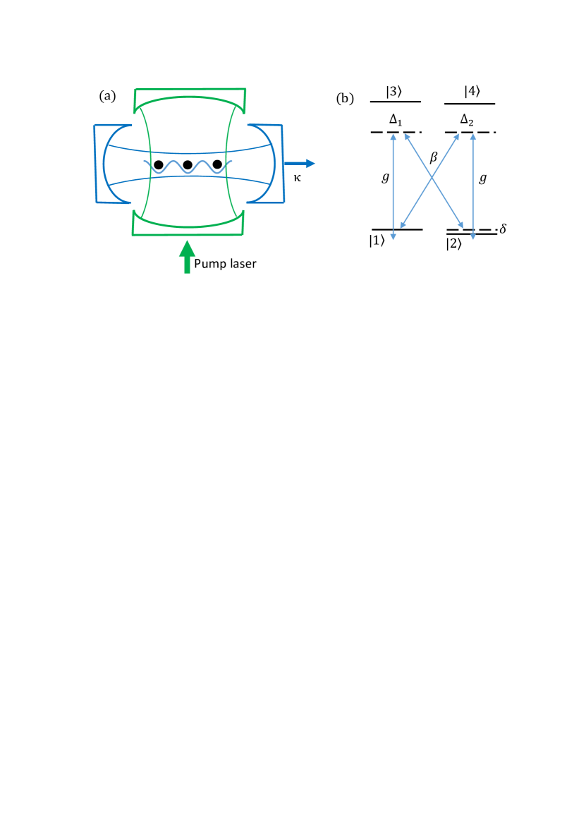
Figure 1: (a) The model system with a 1D chain of atoms with nearest-neighbor interactions in a dissipative cavity and driven by an external transverse field. (b) Energy levels of the atoms and couplings between them by the cavity field and external field. The detunings for the two Raman processes are approximately equal. I.e., $\Delta_{1}\simeq\Delta_{2}\equiv\Delta_{\text{e}}$.

To study the nonequilibrium phase transition in our system, we first shift to the rotating frame defined by the external driving field by applying the operator $U(t)=\exp(-i\omega_{b}a^{{\dagger}}at)$. After the Rotating Wave Approximation (RWA), we obtain the following effective many-body time-independent Hamiltonian,

$$\begin{split}H^{\prime}=&(\Delta-i\frac{\kappa}{2})a^{{\dagger}}a+\frac{g_{0}}{\sqrt{N}}(a^{{\dagger}}e^{i\varphi}+ae^{-i\varphi})\sum_{i}\sigma_{i}^{x}\\ &-\delta\sum_{i}\sigma_{i}^{z}-J\sum_{i}\sigma_{i}^{y}\sigma_{i+1}^{y},\end{split}$$ (2)

where $\Delta=\omega_{a}-\frac{g^{2}}{\Delta_{\text{e}}}-\omega_{b}$ is the mismatch between the cavity and external driving fields, $\kappa$ is the photon loss rate, and $g_{0}=\sqrt{N}g\beta_{0}/\Delta_{\text{e}}$ PhysRevE.67.066203 . The Hamiltonian in Eq. (2), which contains both Ising interactions between the spins and photon leakage out of the cavity, is an interesting and useful model for studying dynamic phase transitions that has not been studied so far.

In Eq. (2), the second term dictates the interaction between the spin chain and the cavity field assisted by the driving of the external field. Because of the leakage of photons out of the cavity, the system evolves irreversibly into a steady state until the effect of driving and dissipation reaches a dynamical equilibrium. Obviously, this steady state has a decisive impact on the physics of both the cavity field and Ising spin chain. To determine the steady state, we expand the field operator $a$ and the spin-chain operator $\sum_{i}\sigma_{i}^{x}$ around their mean field values $\phi_{s}$ and $S_{x}$ in the thermodynamic limit. This allows us to approximate the spin-field interaction term as

$$\begin{split}\frac{(a^{{\dagger}}e^{i\varphi}+ae^{-i\varphi})}{\sqrt{N}}\sum_{i}\sigma_{i}^{x}\approx&\sqrt{N}(a^{{\dagger}}e^{i\varphi}+ae^{-i\varphi})S_{x}\\ &+2\phi_{s}\sum_{i}\sigma_{i}^{x}-2\phi_{s}S_{x}N,\end{split}$$ (3)

where $S_{x}=\frac{1}{N}\langle{\sum_{i}\sigma_{i}^{x}}\rangle_{ss}$ and $\phi_{s}=\frac{1}{2\sqrt{N}}\langle{a^{{\dagger}}e^{i\varphi}+ae^{-i\varphi}}\rangle_{ss}$ are average values evaluated under the steady state. The effective Hamiltonian can then be written as

$$\begin{split}H_{\text{eff}}=&(\Delta-i\frac{\kappa}{2})a^{{\dagger}}a+g_{0}\sqrt{N}(a^{{\dagger}}e^{i\varphi}+ae^{-i\varphi})S_{x}\\ &-2g_{0}\phi_{s}NS_{x}-\sum_{i}\Big{(}\delta\sigma_{i}^{z}-2g_{0}\phi_{s}\sigma_{i}^{x}+J\sigma_{i}^{y}\sigma_{i+1}^{y}\Big{)}.\end{split}$$ (4)

We can now derive the equations of motion for the field operators from $H_{\text{eff}}$,

$$\begin{split}\dot{a}=-i\Delta a-ig_{0}\sqrt{N}S_{x}e^{-i\varphi}-\frac{\kappa}{2}a\\ \dot{a}^{{\dagger}}=i\Delta a^{{\dagger}}+ig_{0}\sqrt{N}S_{x}e^{i\varphi}-\frac{\kappa}{2}a^{{\dagger}},\end{split}$$ (5)

In the steady state ($\frac{d}{dt}a=0$), the mean photon field in cavity is

$$\phi_{s}=-\frac{\Delta g_{0}S_{x}}{\Delta^{2}+\kappa^{2}/4},$$ (6)

which is related to the ground state average $S_{x}$ of the spin part of the Hamiltonian zhang2014quantum . Eq. (6) reveals a critical relation between the field and spin-chain behavior resulting from the dynamic equilibrium. Specifically, macroscopic occupation of cavity photons and macroscopic polarization of the spins in the $x$ direction occur at the same time. Thus, a super-radiant phase transition, if it occurs, may be accompanied by a phase transition in the spin chain between the ferromagnetic and paramagnetic phase. To see how it dictates the system characteristics, we notice that the mean field $\phi_{s}$ in turn has a direct impact on the spin part of the Hamiltonian

$$H_{\text{Ising}}=-\sum_{i}\delta\sigma_{i}^{z}-2g_{0}\phi_{s}\sigma_{i}^{x}+J\sigma_{i}^{y}\sigma_{i+1}^{y}$$ (7)

by modulating the transverse field of the Ising model. The transverse field Ising Hamiltonian in Eq. (7), which has a ferromagnetic phase for a strong Ising interaction $J>B_{\bot}=\sqrt{\delta^{2}+4g_{0}^{2}\phi_{s}^{2}}$, and a paramagnetic phase for a strong transverse field $B_{\bot}>J$, can be solved exactly by the Jordan-Wigner transformation PhysRevLett.95.245701 . Its many-body ground state wave function, $|\Psi_{\text{g}}(\phi_{s})\rangle$, is dependent on the transverse field $B_{\bot}$ of the Ising model and hence on $\phi_{s}$. From $|\Psi_{\text{g}}(\phi_{s})\rangle$, we can calculate the macroscopic polarization in the $x$ direction,

$$S_{x}(\phi_{s})=\frac{1}{N}\langle\Psi_{\text{g}}(\phi_{s})|\sum_{i}\sigma_{i}^{x}|\Psi_{\text{g}}(\phi_{s})\rangle,$$ (8)

which is also dependent on $\phi_{s}$. By solving Eqs. (6) and (8), we can then self-consistently determine the values of $\phi_{s}$ and $S_{x}$ in the dynamical equilibrium.

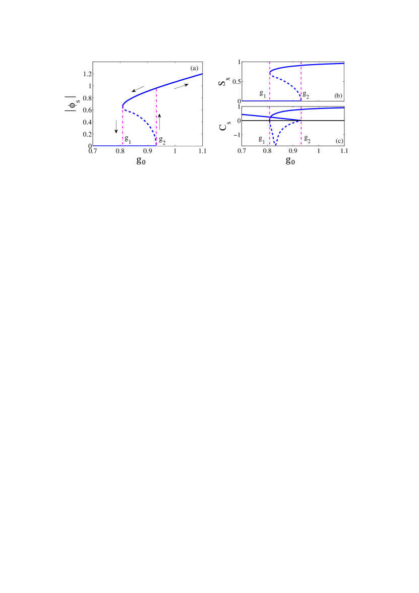
Figure 2: (a) Mean-field cavity photon numbers $\phi_{s}$ versus driving strength $g_{0}$, with a hysteretic regime of bi-stable states. (b) Mean polarization of the spin chain in the $x$ direction $S_{x}$ versus driving strength $g_{0}$, with a stable paramagnetic phase (upper branch) and a stable ferromagnetic phase (lower branch). (c) The stability coefficient $C_{s}$ versus $g_{0}$. In all plots, stable branches are in solid lines and unstable branches are in dashed lines. Other parameters are $\Delta=0.8$, $\delta=0.3$, $\kappa=0.5$, $N=200$. We use $J$ as the energy unit.

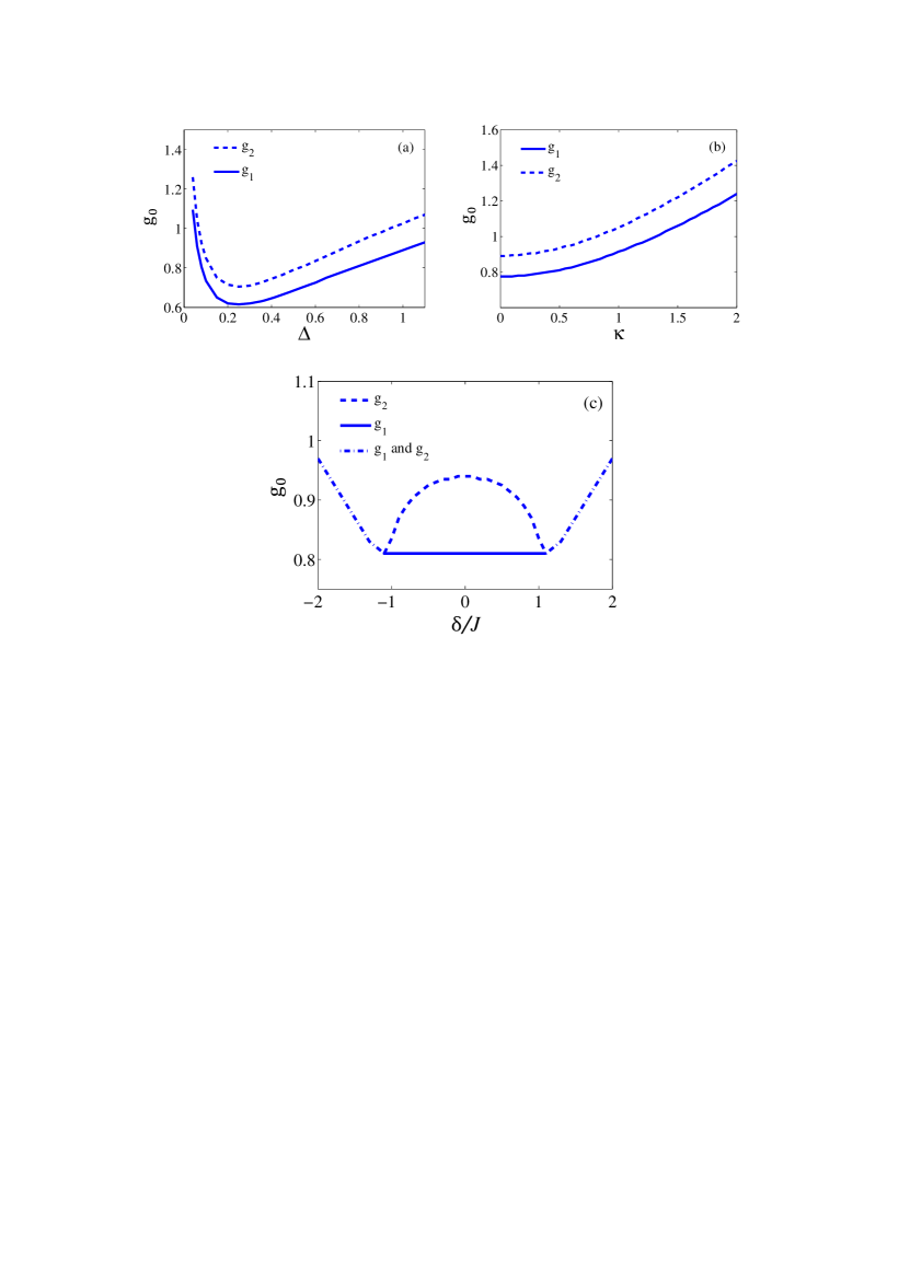
Figure 3: (a) Dependence of the upper and lower critical driving strengths for the phase transitions on the detuning. (b) Dependence of the critical driving strengths on the dissipation rate $\kappa$. (c) Dependence of the critical driving strengths on the ratio between the energy splitting of the spin and the Ising interaction strength, $\delta/J$. The two critical driving strengths become equal for $\delta/J$ greater than 1, indicating the disappearance of the hysteresis in Fig. 2. Other parameters are the same as in Fig. 2 and $J$ is the energy unit.

In Figs. 2 (a) and (b), we plot the solved values for $\phi_{s}$ and $S_{x}$ against the driving strength $g_{0}$ when the spin energy splitting $\delta$ is smaller than the Ising interaction strength $J$. It is seen that, when the coupling is weak, $\phi_{s}=0$, there is no macroscopic photon occupation in the cavity. By Eq. (6), $S_{x}=0$, the spin-chain does not exhibit a macroscopic polarization in the $x$ direction either. When the coupling strength $g_{0}$ increases, $\phi_{s}$ becomes nonzero, indicating that a super-radiant phase transition occurs. However, the solutions of $\phi_{s}$ and $S_{x}$ are not single-valued in a range of driving strength $g_{0}$. The question which solutions are physical can be resolved with a stability analysis.

To study the stability of the solutions for $\phi_{s}$ and $S_{x}$, we consider the time evolution of deviations from their mean field value. We split the field and spin operators into their steady state mean values and small fluctuations

$$a(t)= a_{s}+\delta a(t)$$ (9a)

$$\frac{1}{N}\sum_{i}\sigma_{i}^{x}(t)= S_{x}+\delta S_{x}(t),$$ (9b)

with $a_{s}=\langle a\rangle_{ss}$. Assuming a small fluctuation term for the field value, we have $\phi=\phi_{s}+\delta\phi$ with $\delta\phi=\frac{1}{2\sqrt{N}}(\delta a^{{\dagger}}e^{i\varphi}+\delta ae^{-i\varphi})$, and $\delta S_{x}(t)=\frac{\partial S_{x}}{\partial\phi}\delta\phi$ tian2010circuit . Using the equation of motion for the field operator in Eq. (5), we have

$$\dot{\delta\phi}=-\frac{\kappa}{2}C_{s}\delta\phi,$$ (10)

where

$$C_{s}=1+\frac{g_{0}}{\Delta^{2}+\kappa^{2}/4}\frac{\partial S_{x}}{\partial\phi}$$ (11)

is the stability coefficient. A solution for $\phi_{s}$ is stable if and only if $C_{s}>0$. Therefore, from the plot of $C_{s}$ in Fig. 2(c), we conclude that the branches in solid lines for the solutions of $\phi_{s}$ and $S_{x}$ are stable, whereas the branches in dashed lines are unstable.

From this stability analysis, we can infer that there is a hysteresis in the solutions for $\phi_{s}$ and $S_{x}$ with bi-stability as indicated in Figs. 2 (a) and (b). When the spin-field driving strength $g$ is increased above a critical value $g_{2}$, the value of $\phi_{s}$ jumps from 0 to a nonzero value, and the system makes a discontinuous transition to the super-radiant phase. Likewise, the Ising spin chain experiences a discontinuous phase transition at $g_{2}$ from the ferromagnetic phase to paramagnetic phase, as shown in Fig. 2 (b). Therefore, the phase transitions in our dissipative system are first-order in nature. This is notably different than the conventional transverse field Ising model, in which the quantum phase transition is continuous PhysRevLett.95.245701 . When the system is in the super-radiant phase and the driving strength is decreased, it makes a transition to the vacuum state at a coupling strength $g_{1}$ lower than $g_{2}$, giving rise to the hysteresis in Fig. 2.

Studying the impact of the system’s key parameters on the nature and characteristics of phase transitions can help gain deep insight into our dissipative system. First, we calculate how the critical coupling strengths $g_{1}$ and $g_{2}$ for the phase transitions are dependent on $\Delta$, the effective photon frequency in the effective Hamiltonian in Eq. (2). For a non-dissipative Dicke system, the coupling strength required for the super-radiant phase transition decreases monotonically with the photon frequency zhang2014quantum . As shown in Fig. 3 (a), the behavior of our dissipative system is quite different. Not only do $g_{1}$ and $g_{2}$ reach their minima at a finite value of $\Delta$, but they diverge when $\Delta\rightarrow 0$. This can be understood from Eq. (6), which suggests that the super-radiant phase transition cannot occur for $\Delta=0$ since $\phi_{s}=0$. As for the minimum values of $g_{1}$ and $g_{2}$, we can prove that they occur at $\Delta=\kappa/2$. According to Eq. (6), the values of $g_{1}(\Delta=\kappa/2)$ and $g_{2}(\Delta=\kappa/2)$ are determined by solving

$$\phi_{s}=-\frac{g_{0}S_{x}}{\kappa/2},$$ (12)

with $S_{x}$ determined by the ground state of

$$H_{\text{Ising}}=-\sum_{i}\delta\sigma_{i}^{z}-2g_{0}\phi_{s}\sigma_{i}^{x}+J\sigma_{i}^{y}\sigma_{i+1}^{y}.$$ (13)

For a value of $\Delta$ slightly different, $\Delta=\kappa/2\pm\epsilon$ ($\epsilon\ll\kappa$), $g_{1}(\Delta=\kappa/2\pm\epsilon)$ and $g_{2}(\Delta=\kappa/2\pm\epsilon)$ are determined by solving

$$\phi_{s}^{\prime}=-\frac{g_{0}^{\prime}S_{x}}{\kappa/2},$$ (14)

with $S_{x}$ determined by the ground state of

$$H_{\text{Ising}}=-\sum_{i}\delta\sigma_{i}^{z}-2g_{0}^{\prime}\phi_{s}^{\prime}\sigma_{i}^{x}+J\sigma_{i}^{y}\sigma_{i+1}^{y},$$ (15)

where $g_{0}^{\prime}$ and $\phi_{s}^{\prime}$ are obtained by expansion of Eq. (6) to second order of $\epsilon$ with the results

$$g_{0}^{\prime}=g_{0}\sqrt{1-2\epsilon^{2}/\kappa^{2}}$$ (16)

and

$$\phi_{s}^{\prime}=\frac{\phi_{s}}{\sqrt{1-2\epsilon^{2}/\kappa^{2}}}.$$ (17)

Notice that Eqs. (14) (15) are in the same form with Eqs. (12) (13), indicating that their solutions are related by a proper scaling. Specifically,

$$g_{1}^{\prime}(\Delta=\kappa/2\pm\epsilon)=g_{1}(\Delta=\kappa/2)$$ (18)

with

$$g_{1}^{\prime}(\Delta=\kappa/2\pm\epsilon)\equiv g_{1}(\Delta=\kappa/2\pm\epsilon)\sqrt{1-2\epsilon^{2}/\kappa^{2}}.$$ (19)

Thus we have

$$g_{1}(\Delta=\kappa/2\pm\epsilon)=\frac{g_{1}(\Delta=\kappa/2)}{\sqrt{1-2\epsilon^{2}/\kappa^{2}}}>g_{1}(\Delta=\kappa/2),$$ (20)

and we can conclude that the values of $g_{1}$ and $g_{2}$ are the minimal at $\Delta=\kappa/2$.

Then, we investigate the effect of dissipation rate $\kappa$ on the critical coupling strengths $g_{1}$ and $g_{2}$ for the phase transitions. As shown in Fig. 3 (b), $g_{1}$ and $g_{2}$ increase monotonically with the dissipation rate $\kappa$, suggesting that the phase transitions occur at stronger couplings when the dissipation is more severe. This is understandable, since a higher rate of dissipation must be balanced by stronger driving to support the super-radiant phase. Finally, in Fig. 3 (c), we show how $g_{1}$ and $g_{2}$ change with the relative magnitude of the spin energy splitting $\delta$ and Ising interaction strength $J$. It is seen that, when $\delta$ is smaller than $J$, $g_{1}$ and $g_{2}$ have different values, which suggests discontinuous first-order phase transitions. However, when $\delta$ is greater than $J$, $g_{1}$ and $g_{2}$ are equal. This suggests that the hysteresis in Fig. 2 disappears. Closer examination of the values of $\phi_{s}$ and $S_{x}$ reveals that the phase transitions have become continuous. This behavior is similar to that in closed Dicke systems without dissipation PhysRevLett.93.083001 ; gammelmark2011phase , except that $\delta/J$ needs to be slightly larger than 1 for the phase transitions to become continuous due to the influence of the dissipation.

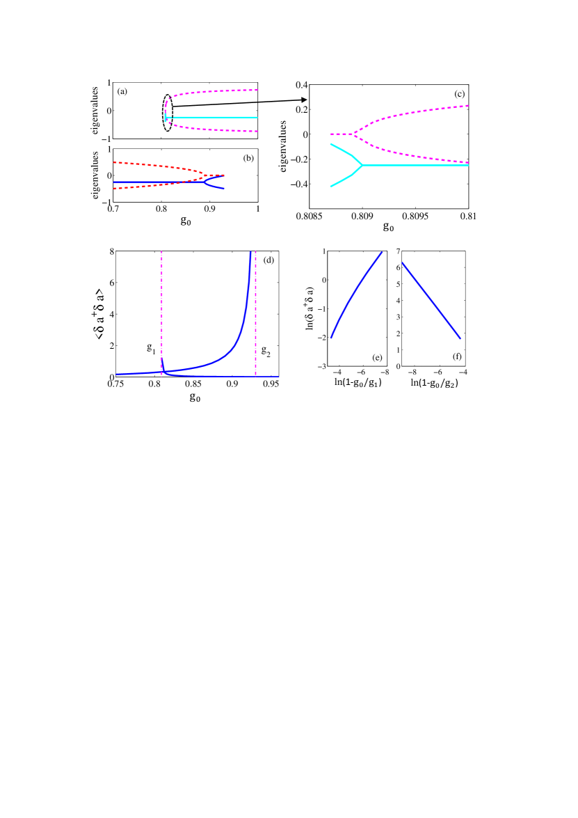
Figure 4: (a) Eigenvalues in Eq. (22) of the linear stability matrix $\mathbf{M}$ for the stable paramagnetic phase. The solid and dashed line are the real and image part respectively. (b) Eigenvalues in Eq. (22) of the linear stability matrix $\mathbf{M}$ for the stable ferromagnetic phase. (c) Closer view of (a) around the critical driving strength $g_{1}$. (d) The number of fluctuating photon number $\langle\delta a^{{\dagger}}\delta a\rangle$ of the steady state when the coupling strength approaches the critical points $g_{1}$ and $g_{2}$. (e) (f) The fluctuating photon number $\langle\delta a^{{\dagger}}\delta a\rangle$ on a log scale. Parameters for the calculation are the same as in Fig. 2 and $J$ is the energy unit.

One more characteristic of the system worth studying is fluctuations because of the crucial role they play in phase transitions binder1987theory ; plischke2006equilibrium . For simplicity, we focus on the fluctuation of the cavity field, and assume that the Ising chain always stays in the ground state corresponding to the cavity field. Under such an assumption, the fluctuation in the spin chain’s polarization in the $x$ direction, $S_{x}$, is $\delta S_{x}(t)=\frac{\partial S_{x}}{\partial\phi}\delta\phi$ to first order in the cavity filed fluctuation $\delta\phi$ tian2010circuit . Denoting the the field fluctuations with $\mathbf{V}=[\delta a,\delta a^{{\dagger}}]^{T}$, and using the equations of motion for the field operators, we have

$$\frac{\partial}{\partial t}\mathbf{V}=\mathbf{M}\mathbf{V}+\widehat{\xi},$$ (21)

where $\widehat{\xi}=(\xi,\xi^{{\dagger}})^{T}$ is the vector of operators for the quantum noise which has zero mean values and whose only non-vanishing correlation is $\langle\xi(t)\xi^{{\dagger}}(t^{\prime})\rangle=\kappa\delta(t-t^{\prime})$. $\mathbf{M}$ is the linear stability matrix of the mean field solution

$$\mathbf{M}=\begin{bmatrix}-i\Delta-i\frac{g_{0}}{2}\frac{\partial S_{x}}{\partial\phi_{s}}-\frac{\kappa}{2}&-i\frac{g_{0}}{2}\frac{\partial S_{x}}{\partial\phi_{s}}\\ i\frac{g_{0}}{2}\frac{\partial S_{x}}{\partial\phi_{s}}&i\Delta+i\frac{g_{0}}{2}\frac{\partial S_{x}}{\partial\phi_{s}}-\frac{\kappa}{2}\end{bmatrix}$$

The matrix $\mathbf{M}$ is non-normal, therefore it has different left and right eigenvectors $\mathbf{R}$, $\mathbf{L}$ PhysRevA.84.043637 , which form a biorthogonal system $\mathbf{L}\mathbf{R}=\mathbf{I}$. $\mathbf{M}$ has two eigenvalues,

$$\omega_{m1}=\frac{-\kappa-i\sqrt{4\Delta^{2}+4\Delta g_{0}\partial S_{x}/\partial\phi}}{2}$$ (22a)

$$\omega_{m2}=\frac{-\kappa+i\sqrt{4\Delta^{2}+4\Delta g_{0}\partial S_{x}/\partial\phi}}{2}.$$ (22b)

which are plotted as a function of driving strength in Figs. 4(a) and (b). When the real part of the eigenvalues is negative, the system is stable PhysRevA.84.043637 . Following the method discussed in Ref. PhysRevA.84.043637 , we solve for the number of fluctuating photon number which is

$$\langle\delta a^{{\dagger}}\delta a\rangle=-\sum_{i,j}\frac{\kappa}{\omega_{mi}+\omega_{mj}}L_{i,1}L_{j,2}R_{2,i}R_{1,j}$$ (23)

where $\omega_{mi}$, $\omega_{mj}$ are the eigenvalues of matrix $\mathbf{M}$. As shown in Fig. 4 (d), when the driving strength decreases and approaches the critical point $g_{1}$ of the system, the photon number fluctuation in the steady state becomes significant, which signals that the photon field enters a normal phase from a super-radiant phase. Likewise, when the driving strength increases and approaches the critical value $g_{2}$, the fluctuation grows quickly. In Figs. 4(e) and (f), we plot the photon fluctuations on a log scale as a function of deviation of the driving strength from the critical point $g_{1}$ and $g_{2}$. The critical exponent can be read from these plots. Near $g_{2}$, it is $-1.0$, consistent with the super-radiant phase transition in a conventional Dicke model without Ising interaction. Near $g_{1}$, the exponent is about $-0.75$.

In summary, we have studied dynamic phase transitions in an open system consisting of an Ising chain in a lossy cavity. When the external driving and cavity leakage reach a dynamic equilibrium, the cavity can undergo a super-radiant phase transition when the driving strength for the Ising chain is strong enough. Interestingly, because of the mutual impact between the Ising chain and cavity field, it is accompanied by a transition between ferromagnetic and paramagnetic phase in the Ising chain. Under certain conditions, the phase transitions are hysteretic and discontinuous, and exhibit different characteristics than those in conventional closed systems. By studying important issues of the system such as stability and fluctuations, we gained valuable insights in the unique properties of quantum phase transitions in driven systems in dynamic equilibrium.

References

- (1) Robert H Dicke. Coherence in spontaneous radiation processes. Physical Review, 93(1):99, 1954.
- (2) Klaus Hepp and Elliott H. Lieb. Equilibrium statistical mechanics of matter interacting with the quantized radiation field. Phys. Rev. A, 8:2517–2525, Nov 1973.
- (3) Neill Lambert, Clive Emary, and Tobias Brandes. Entanglement and the phase transition in single-mode superradiance. Phys. Rev. Lett., 92:073602, Feb 2004.
- (4) Julien Vidal and Sébastien Dusuel. Finite-size scaling exponents in the dicke model. EPL (Europhysics Letters), 74(5):817, 2006.
- (5) Clive Emary and Tobias Brandes. Chaos and the quantum phase transition in the dicke model. Phys. Rev. E, 67:066203, Jun 2003.
- (6) Clive Emary and Tobias Brandes. Quantum chaos triggered by precursors of a quantum phase transition: The dicke model. Phys. Rev. Lett., 90:044101, Jan 2003.
- (7) Kristian Baumann, Christine Guerlin, Ferdinand Brennecke, and Tilman Esslinger. Dicke quantum phase transition with a superfluid gas in an optical cavity. Nature, 464(7293):1301–1306, 2010.
- (8) Ferdinand Brennecke, Rafael Mottl, Kristian Baumann, Renate Landig, Tobias Donner, and Tilman Esslinger. Real-time observation of fluctuations at the driven-dissipative dicke phase transition. Proceedings of the National Academy of Sciences, 110(29):11763–11767, 2013.
- (9) Barry M Garraway. The dicke model in quantum optics: Dicke model revisited. Philosophical Transactions of the Royal Society of London A: Mathematical, Physical and Engineering Sciences, 369(1939):1137–1155, 2011.
- (10) Sam Genway, Weibin Li, Cenap Ates, Benjamin P Lanyon, and Igor Lesanovsky. Generalized dicke nonequilibrium dynamics in trapped ions. Physical review letters, 112(2):023603, 2014.
- (11) LJ Zou, David Marcos, Sebastian Diehl, Stefan Putz, Jörg Schmiedmayer, Johannes Majer, and Peter Rabl. Implementation of the dicke lattice model in hybrid quantum system arrays. Physical review letters, 113(2):023603, 2014.
- (12) Pierre Nataf and Cristiano Ciuti. No-go theorem for superradiant quantum phase transitions in cavity qed and counter-example in circuit qed. Nature communications, 1:72, 2010.
- (13) Michael Scheibner, Thomas Schmidt, Lukas Worschech, Alfred Forchel, Gerd Bacher, Thorsten Passow, and Detlef Hommel. Superradiance of quantum dots. Nature Physics, 3(2):106–110, 2007.
- (14) Sebastian Diehl, Andrea Tomadin, Andrea Micheli, Rosario Fazio, and Peter Zoller. Dynamical phase transitions and instabilities in open atomic many-body systems. Phys. Rev. Lett., 105:015702, Jul 2010.
- (15) Manas Kulkarni, Baris Öztop, and Hakan E. Türeci. Cavity-mediated near-critical dissipative dynamics of a driven condensate. Phys. Rev. Lett., 111:220408, Nov 2013.
- (16) Tony E Lee, Ching-Kit Chan, and Susanne F Yelin. Dissipative phase transitions: Independent versus collective decay and spin squeezing. Physical Review A, 90(5):052109, 2014.
- (17) Jan Gelhausen, Michael Buchhold, Achim Rosch, and Philipp Strack. Quantum-optical magnets with competing short-and long-range interactions: Rydberg-dressed spin lattice in an optical cavity. arXiv preprint arXiv:1608.01319, 2016.
- (18) Lin Tian. Cavity-assisted dynamical quantum phase transition at bifurcation points. Physical Review A, 93(4):043850, 2016.
- (19) D. Nagy, G. Kónya, G. Szirmai, and P. Domokos. Dicke-model phase transition in the quantum motion of a bose-einstein condensate in an optical cavity. Phys. Rev. Lett., 104:130401, Apr 2010.
- (20) D. Nagy, G. Szirmai, and P. Domokos. Critical exponent of a quantum-noise-driven phase transition: The open-system dicke model. Phys. Rev. A, 84:043637, Oct 2011.
- (21) V. M. Bastidas, C. Emary, B. Regler, and T. Brandes. Nonequilibrium quantum phase transitions in the dicke model. Phys. Rev. Lett., 108:043003, Jan 2012.
- (22) MJ Bhaseen, J Mayoh, BD Simons, and J Keeling. Dynamics of nonequilibrium dicke models. Physical Review A, 85(1):013817, 2012.
- (23) Emanuele G. Dalla Torre, Sebastian Diehl, Mikhail D. Lukin, Subir Sachdev, and Philipp Strack. Keldysh approach for nonequilibrium phase transitions in quantum optics: Beyond the dicke model in optical cavities. Phys. Rev. A, 87:023831, Feb 2013.
- (24) Kihwan Kim, M-S Chang, S Korenblit, R Islam, EE Edwards, JK Freericks, G-D Lin, L-M Duan, and C Monroe. Quantum simulation of frustrated ising spins with trapped ions. Nature, 465(7298):590–593, 2010.
- (25) K Kim, S Korenblit, R Islam, EE Edwards, MS Chang, C Noh, H Carmichael, GD Lin, LM Duan, CC Joseph Wang, et al. Quantum simulation of the transverse ising model with trapped ions. New Journal of Physics, 13(10):105003, 2011.
- (26) AO Niskanen, K Harrabi, F Yoshihara, Y Nakamura, S Lloyd, and JS Tsai. Quantum coherent tunable coupling of superconducting qubits. Science, 316(5825):723–726, 2007.
- (27) Chiu Fan Lee and Neil F. Johnson. First-order superradiant phase transitions in a multiqubit cavity system. Phys. Rev. Lett., 93:083001, Aug 2004.
- (28) Søren Gammelmark and Klaus Mølmer. Phase transitions and heisenberg limited metrology in an ising chain interacting with a single-mode cavity field. New Journal of Physics, 13(5):053035, 2011.
- (29) Yu-Na Zhang, Xi-Wang Luo, Guang-Can Guo, Zheng-Wei Zhou, and Xingxiang Zhou. Quantum phase transition of nonlocal ising chain with transverse field in a resonator. Physical Review B, 90(9):094510, 2014.
- (30) Yu Chen, Zhenhua Yu, and Hui Zhai. Quantum phase transitions of the bose-hubbard model inside a cavity. Physical Review A, 93(4):041601, 2016.
- (31) F. Dimer, B. Estienne, A. S. Parkins, and H. J. Carmichael. Proposed realization of the dicke-model quantum phase transition in an optical cavity qed system. Phys. Rev. A, 75:013804, Jan 2007.
- (32) Jens Klinder, H Keßler, M Reza Bakhtiari, M Thorwart, and A Hemmerich. Observation of a superradiant mott insulator in the dicke-hubbard model. Physical review letters, 115(23):230403, 2015.
- (33) Renate Landig, Lorenz Hruby, Nishant Dogra, Manuele Landini, Rafael Mottl, Tobias Donner, and Tilman Esslinger. Quantum phases from competing short-and long-range interactions in an optical lattice. Nature, 532(7600):476–479, 2016.
- (34) L-M Duan, E Demler, and MD Lukin. Controlling spin exchange interactions of ultracold atoms in optical lattices. Physical review letters, 91(9):090402, 2003.
- (35) L Tian. Circuit qed and sudden phase switching in a superconducting qubit array. Physical review letters, 105(16):167001, 2010.
- (36) Jacek Dziarmaga. Dynamics of a quantum phase transition: Exact solution of the quantum ising model. Phys. Rev. Lett., 95:245701, Dec 2005.
- (37) Kurt Binder. Theory of first-order phase transitions. Reports on progress in physics, 50(7):783, 1987.
- (38) Michael Plischke and Birger Bergersen. Equilibrium statistical physics. World Scientific Publishing, Singapore, 2006.