Voltage stabilization in DC microgrids: an approach based on line-independent plug-and-play controllers

Abstract

We consider the problem of stabilizing voltages in DC microGrids (mGs) given by the interconnection of Distributed Generation Units (DGUs), power lines and loads. We propose a decentralized control architecture where the primary controller of each DGU can be designed in a Plug-and-Play (PnP) fashion, allowing the seamless addition of new DGUs. Differently from several other approaches to primary control, local design is independent of the parameters of power lines. Moreover, differently from the PnP control scheme in [1], the plug-in of a DGU does not require to update controllers of neighboring DGUs. Local control design is cast into a Linear Matrix Inequality (LMI) problem that, if unfeasible, allows one to deny plug-in requests that might be dangerous for mG stability. The proof of closed-loop stability of voltages exploits structured Lyapunov functions, the LaSalle invariance theorem and properties of graph Laplacians. Theoretical results are backed up by simulations in PSCAD.

1 Introduction

DC mGs are networks combining energy sources, interfaced through converters, and loads connected through power lines. As DC mGs can be coupled to the main grid through AC-DC converters only, they can be thought as always operating in islanded mode. This is due to the fact that converters have finite power rating, which can limit substantially the power transfer.

Motivated by advances in power electronics, batteries and renewable DC sources, DC mGs find nowadays applications in various field such as high-efficiency households, electric vehicles, hybrid energy storage systems, data centers, avionics and marine systems [2].

In order to operate DC mGs in a safe and reliable way, several challenges must be addressed. A central one is to provide voltage stability [3, 4, 5, 6, 1, 7]. This property is fundamental and should be guaranteed even in presence of unreliable communication channels among local controllers or DGUs. This promoted the study of decentralized control architectures at the primary level of the mG control hierarchy [8]. The most popular solutions are based on droop controllers for each DGU, built on top inner voltage and current loops [8]. Stability of droop control has been however shown either for specific mG topologies [9] or for general topologies, but relying on networked secondary regulators [5].

An alternative class of decentralized primary controllers, termed PnP according to the terminology used in [10, 11] and [12], has been proposed in [1, 7]. The main feature of the PnP approach is to allow the addition and removal of DGUs independently of the mG size and without retuning all local controllers.

In particular, in [1, 7], the computation of a local controller requires to solve an LMI problem based only on information about the corresponding DGU and power lines connecting neighboring DGUs. This has two consequences. First, if a DGU is plugged-in, its neighbors must update their controllers through LMIs, as they will be connected to new lines. Second, in order to preserve stability of the mG, the plug-in of the DGU must be denied if one of the LMI problems is infeasible. Another feature of PnP control is that LMIs give, as a byproduct, local structured Lyapunov functions that can be used for certifying asymptotic stability of the whole mG.

The dependence of a local controller on power line parameters can be critical when they are not precisely known. This problem has been considered in [13] and [14] where line-independent controllers have been proposed. However, in [13] and [14] voltage stability has been studied only for mGs with at most four DGUs.

In this paper, we propose a variant of the PnP design algorithm in [1, 7]. The main novelty is that the design of local controllers is line-independent and the only global quantity used in the synthesis algorithm is a scalar parameter. As a consequence, even if a DGU wants to plug -in or -out, its neighbors do not have to update local controllers. This considerably simplifies the plug-in protocol described in [1, 7], as switching of local controllers is avoided and bumpless control architectures (for avoiding abrupt changes in the control variables) are unnecessary. Moreover, the new design procedure better complies with privacy requirements of energy markets where DGUs can have different owners. Indeed, the addition of new DGUs does not require other stakeholders to disclose models of their own DGUs or change their operation. For the new design procedure, the structure of each local controller is identical to the one proposed in [1, 7]. Also LMI problems associated to control design are similar to those in [1, 7]. However, the proof of asymptotic stability of the closed-loop system is substantially different and more involved. In particular, it is based on the fact that, under Quasi Stationary Line (QSL) approximations, electrical coupling among DGUs can be described by graph Laplacians [15]. This feature, together with the use of structured Lyapunov functions and the LaSalle Invariance principle [16], allows us to derive the desired result.

The paper is structured as follows. Results from [1, 7] about the DGU model and the structure of PnP controllers are summarized in Sections 2 and 3.1. The new PnP approach to the design of local controllers is described in Sections 3.2, 3.3 and 3.4, along with the stability analysis of the closed-loop system. Simulations in PSCAD using a 5-DGU mG and illustrating the plug-in of an additional DGU are described in Section 4.

Notation. We use $P>0$ (resp. $P\geq 0$) for indicating the real symmetric matrix $P$ is positive-definite (resp. positive-semidefinite). Let $A\in\mathbb{R}^{n\times m}$ be a matrix inducing the linear map $A:\mathbb{R}^{m}\rightarrow\mathbb{R}^{n}$. The image and the nullspace (or kernel) of $A$ are indicated with $\text{Im}(A)$ and $\text{Ker}(A)$, respectively. The symbol $\oplus$ refers to the sum of subspaces that are orthogonal (also called orthogonal direct sum).

2 DC Microgrid model

2.1 DGU electrical model

In this section, we describe the electrical model of a DC mG considered in [1, 7]. The electrical scheme of the $i$-th DGU represented within the dashed frame in Figure 1.

The DC voltage source represents a generic renewable resource and a Buck converter is commanded in order to supply a local DC load connected to the Point of Common Coupling (PCC) through a series $RL$ filter. We also assume that loads are unknown and act as current disturbances ($I_{L}$) [1, 7, 17]. Let us consider an mG composed of $N$ DGUs and let ${\mathcal{D}}=\{1,\dots,N\}$. We call two DGUs neighbors if there is a power line connecting them and denote with ${\mathcal{N}}_{i}\subset{\mathcal{D}}$ the subset of neighbors of DGU $i$. The neighboring relation is symmetric: $j\in{\mathcal{N}}_{i}$ implies $i\in{\mathcal{N}}_{j}$. Furthermore, let $\mathcal{E}=\{(i,j):$ $i\in{\mathcal{D}},$ $j\in{\mathcal{N}}_{i}\}$ collect unordered pairs of indices associated to lines. The topology of the mG is then described by the undirected graph ${\mathcal{G}}_{el}$ with nodes ${\mathcal{D}}$ and edges ${\mathcal{E}}$.

From Figure 1, by applying Kirchoff’s voltage and current laws, and exploiting QSL approximation of power lines [18, 1, 7], we obtain the following model of DGU $i$

$$\text{DGU}~{}i:\quad\left\{\begin{aligned} \frac{dV_{i}}{dt}&=\frac{1}{C_{ti}}I_{ti}+\sum\limits_{j\in{\mathcal{N}}_{i}}\left(\frac{V_{j}}{C_{ti}R_{ij}}-\frac{V_{i}}{C_{ti}R_{ij}}\right)-\frac{1}{C_{ti}}I_{Li}\\ \frac{dI_{ti}}{dt}&=-\frac{1}{L_{ti}}V_{i}-\frac{R_{ti}}{L_{ti}}I_{ti}+\frac{1}{L_{ti}}V_{ti}\\ \end{aligned}\right.$$ (1)

where variables $V_{i}$, $I_{ti}$, are the $i$-th PCC voltage and filter current, respectively, $V_{ti}$ represents the command to the Buck converter, and $R_{ti}$, $L_{ti}$ and $C_{ti}$ the converter electrical parameters. Moreover, $V_{j}$ is the voltage at the PCC of each neighboring DGU $j\in{\mathcal{N}}_{i}$ and $R_{ij}$ is the resistance of the power DC line connecting DGUs $i$ and $j$.

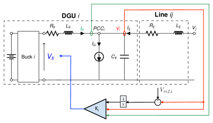
Figure 1: Electrical scheme of DGU $i$ (in the dashed frame) and local PnP voltage controller.

Remark 1.

Model (1) hinges on three main assumptions. First, Buck converter dynamics, that are inherently switching, have been averaged over time. This is however a mild approximation for modern converters that can operate at very high frequencies. Second, QSL approximations have been used. They amount to assume that power lines are mainly resistive and they have been justified in terms of singular perturbation theory [1]. Third, loads are connected at the PCC of each DGU. It has been shown that general interconnections of loads and DGUs can always be mapped into this topology using a network reduction method known as Kron reduction [15].

2.2 State-space model of the mG

Dynamics (1) can be written in terms of state-space variables as follows

$$\text{ ${\Sigma}_{[i]}^{DGU}:$}\left\{\begin{aligned} {\dot{x}}_{[i]}(t)&=A_{ii}{x}_{[i]}(t)+B_{i}{u}_{[i]}(t)+M_{i}{d}_{[i]}(t)+{\xi}_{[i]}(t)\\ {z}_{[i]}(t)&=H_{i}{x}_{[i]}(t)\\ \end{aligned}\right.$$

where ${x}_{[i]}=[V_{i},I_{ti}]^{T}$ is the state, ${u}_{[i]}=V_{ti}$ the control input, ${d}_{[i]}=I_{Li}$ the exogenous input and ${z}_{[i]}=V_{i}$ the controlled variable of the system. The term ${\xi}_{[i]}=\sum_{j\in{\mathcal{N}}_{i}}A_{ij}({x}_{[j]}-{x}_{[i]})$ accounts for the coupling with each DGU $j\in{\mathcal{N}}_{i}$. This model is identical to the one provided in [1, 7], except that all coupling terms have been embedded in variables ${\xi}_{[i]}$. The matrices of ${\Sigma}_{[i]}^{DGU}$ are obtained from (1) as:

$$A_{ii}=\begin{bmatrix}0&\frac{1}{C_{ti}}\\ -\frac{1}{L_{ti}}&-\frac{R_{ti}}{L_{ti}}\\ \end{bmatrix},\hskip 8.53581ptA_{ij}=\begin{bmatrix}\frac{1}{R_{ij}C_{ti}}&0\\ 0&0\end{bmatrix},$$

$$B_{i}=\begin{bmatrix}0\\ \frac{1}{L_{ti}}\end{bmatrix},\qquad M_{i}=\begin{bmatrix}-\frac{1}{C_{ti}}\\ 0\\ \end{bmatrix},\qquad H_{i}=\begin{bmatrix}1&0\end{bmatrix}.$$

The overall mG model is given by

$$\mathbf{\dot{x}}(t) =\mathbf{Ax}(t)+\mathbf{Bu}(t)+\mathbf{Md}(t)$$ (2)

$$\mathbf{z}(t) =\mathbf{Hx}(t)$$

where $\mathbf{x}=({x}_{[1]},\ldots,{x}_{[N]})\in\mathbb{R}^{2N}$, $\mathbf{u}=({u}_{[1]},\ldots,{u}_{[N]})\in\mathbb{R}^{N}$, $\mathbf{d}=({d}_{[1]},\ldots,{d}_{[N]})\in\mathbb{R}^{N}$, $\mathbf{z}=({z}_{[1]},\ldots,{z}_{[N]})\in\mathbb{R}^{N}$. Matrices $\mathbf{A}$, $\mathbf{B}$, $\mathbf{M}$ and $\mathbf{H}$ are reported in Appendix A.2 and A.3 of [7].

3 Design of stabilizing voltage controllers

3.1 Structure of local controllers

Let $\mathbf{z_{ref}}(t)$ be the desired reference trajectory for the output $\mathbf{z}(t)$. As in [1, 7], in order to track constant references $\mathbf{z_{ref}}(t)=\mathbf{\bar{z}_{ref}}$, when $\mathbf{d}(t)=\mathbf{\bar{d}}$ is constant as well, we augment the mG model with integrators [19]. A necessary condition for steering to zero the error $\mathbf{e}(t)=\mathbf{z_{ref}}(t)-\mathbf{z}(t)$ as $t\rightarrow\infty$, is that, for arbitrary $\mathbf{\bar{d}}$ and $\mathbf{\bar{z}_{ref}}$, there are equilibrium states and inputs $\mathbf{\bar{x}}$ and $\mathbf{\bar{u}}$ verifying (2).

The existence of these equilibria can be shown following the proof of Proposition 1 in [1].

The dynamics of the integrators is (see Figure 1, where $z_{ref_{[i]}}=V_{ref,i}$)

$${\dot{v}}_{[i]}(t)={e}_{[i]}(t) ={z_{ref}}_{[i]}(t)-{z}_{[i]}(t)$$ (3)

$$={z_{ref}}_{[i]}(t)-H_{i}{x}_{[i]}(t),$$

and hence, the augmented DGU model is

$${\hat{\Sigma}}_{[i]}^{DGU}:\left\{\begin{aligned} {\dot{\hat{x}}}_{[i]}(t)&=\hat{A}_{ii}{\hat{x}}_{[i]}(t)+\hat{B}_{i}{u}_{[i]}(t)+\hat{M}_{i}{\hat{d}}_{[i]}(t)+{\hat{\xi}}_{[i]}(t)\\ {z}_{[i]}(t)&=\hat{H}_{i}{\hat{x}}_{[i]}(t)\end{aligned}\right.$$ (4)

where ${\hat{x}}_{[i]}=[{x^{T}}_{[i]},v_{i,}]^{T}\in\mathbb{R}^{3}$ is the state, ${\hat{d}}_{[i]}=[{d}_{[i]},{z_{ref}}_{[i]}]^{T}\in\mathbb{R}^{2}$ collects the exogenous signals and ${\hat{\xi}}_{[i]}=\sum_{j\in{\mathcal{N}}_{i}}\hat{A}_{ij}({\hat{x}}_{[j]}-{\hat{x}}_{[i]})$. Matrices in (4) are defined as follows

$$\hat{A}_{ii} =\begin{bmatrix}A_{ii}&0\\ -H_{i}C_{i}&0\end{bmatrix},\hat{A}_{ij}=\begin{bmatrix}A_{ij}&0\\ 0&0\end{bmatrix},\hat{B}_{i}=\begin{bmatrix}B_{i}\\ 0\end{bmatrix},$$

$$\hat{M}_{i} =\begin{bmatrix}M_{i}&0\\ 0&1\end{bmatrix},\hskip 14.22636pt\hat{H}_{i}=\begin{bmatrix}H_{i}&0\end{bmatrix}.$$

As in Proposition 2 of [1], one can show that positivity of electrical parameters guarantees that the pair $(\hat{A}_{ii},\hat{B}_{i})$ is controllable. Hence, system (4) can be stabilized.

The overall augmented system is obtained from (4) as

$$\left\{\begin{aligned} \mathbf{\dot{\hat{x}}}(t)&=\mathbf{\hat{A}\hat{x}}(t)+\mathbf{\hat{B}u}(t)+\mathbf{\hat{M}\hat{d}}(t)\\ \mathbf{z}(t)&=\mathbf{\hat{H}\hat{x}}(t)\end{aligned}\right.$$ (5)

where $\mathbf{\hat{x}}$ and $\mathbf{\hat{d}}$ collect variables ${\hat{x}}_{[i]}$ and ${\hat{d}}_{[i]}$ respectively, and matrices $\mathbf{\hat{A}},\mathbf{\hat{B}},\mathbf{\hat{M}}$ and $\mathbf{\hat{H}}$ are obtained from systems (4).

Now we equip each DGU ${\hat{\Sigma}}_{[i]}^{DGU}$ with the following state-feedback controller

$${{\mathcal{C}}}_{[i]}:\qquad{u}_{[i]}(t)=K_{i}{\hat{x}}_{[i]}(t)$$ (6)

where $K_{i}=\left[k_{1,i}\text{ }k_{2,i}\text{ }k_{3,i}\right]\in\mathbb{R}^{1\times 3}$. It turns out that, together with the integral action (3), controllers ${{\mathcal{C}}}_{[i]}$, define a multivariable PI regulator, see Figure 1. In particular, the overall control architecture is decentralized since the computation of ${u}_{[i]}$ requires the state of ${\hat{\Sigma}}_{[i]}^{DGU}$ only. It is important to highlight that, in general, decentralized design of local regulators can fail to guarantee voltage stability of the whole mG, if couplings among DGUs are neglected during the design phase (see Appendix A). In the sequel, we show how structured Lyapunov functions can be used to ensure asymptotic stability of the whole mG, when DGUs are equipped with controllers (6).

3.2 Conditions for stability of the closed-loop mG

In absence of coupling terms ${\hat{\xi}}_{[i]}(t)$, one would like to guarantee asymptotic stability of the nominal closed-loop subsystem

$${\dot{\hat{x}}}_{[i]}(t)=\underbrace{(\hat{A}_{ii}+\hat{B}_{i}K_{i})}_{F_{i}}{\hat{x}}_{[i]}(t)+\hat{M}_{i}{{\hat{d}}}_{[i]}(t).\\$$ (7)

By direct calculation, one can show that $F_{i}$ has the following structure

$$F_{i} =\left[\begin{array}[]{c|cc}0&f_{12,i}&0\\ \hline\cr f_{21,i}&f_{22,i}&f_{23,i}\\ f_{13,i}&0&0\end{array}\right]=$$ (8)

$$=\left[\begin{array}[]{c|cc}0&\frac{1}{C_{t}}&0\\ \hline\cr\frac{(k_{i,1}-1)}{L_{ti}}&\frac{(k_{i,2}-R_{ti})}{L_{ti}}&\frac{k_{i,3}}{L_{ti}}\\ -1&0&0\end{array}\right]=\left[\begin{array}[]{c|cc}0&{\mathcal{F}}_{12,i}\\ \hline\cr{\mathcal{F}}_{21,i}&{\mathcal{F}}_{22,i}\end{array}\right].$$

From Lyapunov theory, asymptotic stability of (7) is equivalent to the existence of a Lyapunov function ${\mathcal{V}}_{i}({{\hat{x}}}_{[i]})={{\hat{x}}}_{[i]}^{T}P_{i}{{\hat{x}}}_{[i]}$ where $P_{i}\in\mathbb{R}^{3\times 3}$, $P=P^{T}>0$ and

$$Q_{i}=F_{i}^{T}P_{i}+P_{i}F_{i}$$ (9)

is negative definite. In presence of nonzero coupling terms, we will show that asymptotic stability can be achieved under two additional conditions. The first one is the use of the following separable Lyapunov functions

$${\mathcal{V}}_{i}(\hat{x}_{[i]})=\eta_{i}\hat{x}_{[i],1}^{2}+[\hat{x}_{[i],2}\text{ }\hat{x}_{[i],3}]{\mathcal{P}}_{22,i}[\hat{x}_{[i],2}\text{ }\hat{x}_{[i],3}]^{T},$$

where

$${\mathcal{P}}_{22,i}=\left[\begin{array}[]{cc}p_{22,i}&p_{23,i}\\ p_{23,i}&p_{33,i}\end{array}\right].$$ (10)

This requirement is summarized in the next assumption.

Assumption 1.

Gains $K_{i}$, $i\in{\mathcal{D}}$ are designed such that, in (9), the positive definite matrix $P_{i}$ has the structure

$$P_{i}=\left[\begin{array}[]{c|c}\eta_{i}&\mathbf{0}_{1\times 2}\\ \hline\cr\mathbf{0}_{2\times 1}&{\mathcal{P}}_{22,i}\\ \end{array}\right],$$ (11)

where the entries of ${\mathcal{P}}_{22,i}$ are arbitrary and $\eta_{i}>0$ is a local parameter.

The second condition concerns the values of parameters $\eta_{i}$.

Assumption 2.

Given a constant $\bar{\sigma}>0$ (a parameter common to all DGUs), parameters $\eta_{i}$ in (11) are given by

$$\eta_{i}=\bar{\sigma}C_{ti}\hskip 19.91692pt\forall i\in{\mathcal{D}}.$$ (12)

The next result shows that, under Assumption 1, Lyapunov theory certifies, at most, marginal stability of (7).

Proposition 1.

Under Assumption 1, the matrix $Q_{i}$ cannot be negative definite. Moreover, if

$$Q_{i}\leq 0,$$ (13)

then $Q_{i}$ has the following structure:

$$Q_{i}=\left[\begin{array}[]{c|cc}0&0&0\\ \hline\cr 0&q_{22,i}&q_{23,i}\\ 0&q_{23,i}&q_{33,i}\\ \end{array}\right]=\left[\begin{array}[]{c|cc}0&\mathbf{0}_{1\times 2}\\ \hline\cr\mathbf{0}_{2\times 1}&Q_{22,i}\end{array}\right].$$ (14)

Proof.

By direct computation, from (8) and (11) one has $q_{11,i}=0$, showing that $Q_{i}$ cannot be negative definite, as its first minor is not positive. Moreover, if a negative semidefinite matrix has a zero element on its diagonal, then the corresponding row and column have zero entries. This basic property can be shown as follows. If ${\mathcal{Q}}\in\mathbb{R}^{n\times n}$ is symmetric and negative semidefinite, then $x^{T}{\mathcal{Q}}x\leq 0$, $\forall x\in\mathbb{R}^{n}$. Partitioning ${\mathcal{Q}}$ and $x$ as

$${\mathcal{Q}}=\left[\begin{array}[]{c|cc}{\mathcal{Q}}_{11}&\widetilde{{\mathcal{Q}}}^{T}\\ \hline\cr\widetilde{{\mathcal{Q}}}&\widehat{{\mathcal{Q}}}\end{array}\right]\hskip 14.22636ptx=\left[\begin{array}[]{c}x_{11}\\ \tilde{x}\end{array}\right],$$

one obtains

$$x^{T}{\mathcal{Q}}x=x_{11}^{2}{\mathcal{Q}}_{11}+2x_{11}\widetilde{{\mathcal{Q}}}^{T}\tilde{x}+\tilde{x}^{T}\widehat{{\mathcal{Q}}}\tilde{x}.$$

Without loss of generality, assume ${\mathcal{Q}}_{11}=0$. Then, for any $x$ with $\tilde{x}=0$ and $x_{11}\neq 0$, one has $x^{T}{\mathcal{Q}}x=0$, i.e. $x$ is a maximizer of $x^{T}{\mathcal{Q}}x.$ Consequently, it must hold $\frac{\mathrm{d}}{\mathrm{dt}}\left(x^{T}{\mathcal{Q}}x\right)=0$, i.e. $2{\mathcal{Q}}x=0$, yielding

$$\left\{\begin{aligned} {\mathcal{Q}}_{11}x_{11}+\widetilde{{\mathcal{Q}}}^{T}\tilde{x}&=0\\ \widetilde{{\mathcal{Q}}}x_{11}+\widehat{{\mathcal{Q}}}\tilde{x}&=0\\ \end{aligned}\right.$$

Using ${\mathcal{Q}}_{11}=0$ and $\tilde{x}=0$, the previous linear system reduces to $\widetilde{{\mathcal{Q}}}x_{11}=0$, that implies $\widetilde{{\mathcal{Q}}}=0$. Concluding, (13) implies (14). ∎

Consider now the overall closed-loop mG model

$$\left\{\begin{aligned} \mathbf{\dot{\hat{x}}}(t)&=(\mathbf{\hat{A}+\hat{B}K})\mathbf{\hat{x}}(t)+\mathbf{\hat{M}{\hat{d}}}(t)\\ \mathbf{z}(t)&=\mathbf{\hat{H}\hat{x}}(t)\end{aligned}\right.$$ (15)

obtained by combining (5) and (6), with $\mathbf{K}={\mbox{diag}}(K_{1},\dots,K_{N})$. Consider also the collective Lyapunov function

$${\mathcal{V}}(\mathbf{{\hat{x}}})=\sum_{i=1}^{N}{\mathcal{V}}_{i}(\hat{x}_{[i]})=\mathbf{{\hat{x}}}^{T}\mathbf{P}\mathbf{{\hat{x}}}$$ (16)

where $\mathbf{P}={\mbox{diag}}(P_{1},\dots,P_{N})$. One has $\dot{\mathcal{V}}(\mathbf{{\hat{x}}})=\mathbf{{\hat{x}}}^{T}\mathbf{Q}\mathbf{{\hat{x}}}$ where

$$\mathbf{Q}=(\mathbf{\hat{A}}+\mathbf{\hat{B}K})^{T}\mathbf{P}+\mathbf{P}(\mathbf{\hat{A}}+\mathbf{\hat{B}K}).$$

A consequence of Proposition 1 is that, under Assumption 1, the matrix $\mathbf{Q}$ cannot be negative definite. At most, one has

$$\mathbf{Q}\leq 0.$$ (17)

Moreover, even if (13) holds for all $i\in{\mathcal{D}}$, the inequality (17) might be violated because of the nonzero coupling terms $\hat{A}_{ij}$ in matrix $\mathbf{\hat{A}}$. The next result shows that this cannot happen under Assumption 2.

Proposition 2.

Under Assumptions 1 and 2, if gains $K_{i}$ are computed in order to fulfill (13) for all $i\in{\mathcal{D}}$, then (17) holds.

Proof.

Consider the following decomposition of matrix $\mathbf{\hat{A}}$

$$\mathbf{\hat{A}}=\mathbf{\hat{A}_{D}}+\mathbf{\hat{A}_{\Xi}}+\mathbf{\hat{A}_{C}},$$ (18)

where $\mathbf{\hat{A}_{D}}={\mbox{diag}}(\hat{A}_{ii},\dots,\hat{A}_{NN})$ collects the local dynamics only, while $\mathbf{\hat{A}_{\Xi}}={\mbox{diag}}(\hat{A}_{\xi 1},\dots,\hat{A}_{\xi N})$ with

$$\hat{A}_{\xi i}=\begin{bmatrix}-\sum\limits_{j\in{\mathcal{N}}_{i}}\frac{1}{R_{ij}C_{ti}}&0&0\\ 0&0&0\\ 0&0&0\end{bmatrix},$$

takes into account the dependence of each local state on the neighboring DGUs. We want to prove (17), that, according to the decomposition (18), is equivalent to show that

$$\underbrace{\mathbf{(\hat{A}_{D}+\hat{B}K)^{T}P+P(\hat{A}_{D}+\hat{B}K)+}}_{({a})}\underbrace{\mathbf{2\hat{A}_{\Xi}P}}_{(b)}+\underbrace{\mathbf{\hat{A}_{C}}^{T}\mathbf{P+P\hat{A}_{C}}}_{(c)}\leq 0.$$ (19)

By means of (13), matrix $(a)=\mathrm{diag}(Q_{1},\dots,Q_{N})$ is negative semidefinite. Now, let us study the contribution of $(b)+(c)$ in (19). Matrix $(b)$, by construction, is block diagonal and collects on its diagonal blocks in the form

$$2{\hat{A}}_{\xi i}P_{i} =\begin{bmatrix}-2\sum\limits_{j\in{\mathcal{N}}_{i}}\frac{1}{R_{ij}C_{ti}}&0&0&\\ 0&0&0\\ 0&0&0\\ \end{bmatrix}\left[\begin{array}[]{c|c}\eta_{i}&\mathbf{0}_{1\times 2}\\ \hline\cr\mathbf{0}_{2\times 1}&{\mathcal{P}}_{22,i}\end{array}\right]=$$ (20)

$$=\begin{bmatrix}-2\sum\limits_{j\in{\mathcal{N}}_{i}}\tilde{\eta}_{ij}&0&0\\ 0&0&0\\ 0&0&0\\ \end{bmatrix},$$

where

$$\tilde{\eta}_{ij}=\frac{\eta_{i}}{R_{ij}C_{ti}}.$$ (21)

As regards matrix $(c)$, we have that each the block in position $(i,j)$ is equal to

$$\left\{\begin{array}[]{ll}P_{i}\hat{A}_{ij}+\hat{A}_{ji}^{T}P_{j}&\hskip 19.91692pt\mbox{if }j\in\mathcal{N}_{i}\\ 0&\hskip 19.91692pt\mbox{otherwise}\end{array}\right.$$

where

$$P_{i}\hat{A}_{ij}+\hat{A}_{ji}^{T}P_{j} =\begin{bmatrix}\tilde{\eta}_{ij}+\tilde{\eta}_{ji}&0&0\\ 0&0&0\\ 0&0&0\\ \end{bmatrix}.$$ (22)

From (20) and (22), we notice that only the elements in position $(1,1)$ of each $3\times 3$ block of $(b)+(c)$ can be different from zero. Hence, in order to evaluate the positive/negative definiteness of the $3N\times 3N$ matrix $(b)+(c)$, we can equivalently consider the $N\times N$ matrix

$${\mathcal{L}}=\left[\begin{array}[]{cccc}-2\sum\limits_{j\in{\mathcal{N}}_{1}}\tilde{\eta}_{1j}&\bar{\eta}_{12}&\dots&\bar{\eta}_{1N}\\ \bar{\eta}_{21}&\ddots&\ddots&\vdots\\ \vdots&\ddots&-2\sum\limits_{j\in{\mathcal{N}}_{N-1}}\tilde{\eta}_{N-1j}&\bar{\eta}_{N-1N}\\ \bar{\eta}_{N1}&\dots&\bar{\eta}_{NN-1}&-2\sum\limits_{j\in{\mathcal{N}}_{N}}\tilde{\eta}_{Nj}\end{array}\right],$$ (23)

obtained by deleting the second and third row and column in each block of $(b)+(c)$. One has ${\mathcal{L}}={\mathcal{M}}+{\mathcal{G}}$, where

$$\mathcal{M}=\begin{bmatrix}-2\sum\limits_{j\in{\mathcal{N}}_{1}}\tilde{\eta}_{1j}&0&\dots&0\\ 0&-2\sum\limits_{j\in{\mathcal{N}}_{2}}\tilde{\eta}_{2j}&\ddots&\vdots\\ \vdots&\ddots&\ddots&0\\ 0&\dots&0&-2\sum\limits_{j\in{\mathcal{N}}_{N}}\tilde{\eta}_{Nj}\end{bmatrix}$$

and

$$\mathcal{G}=\left[\begin{array}[]{cccc}0&\bar{\eta}_{12}&\dots&\bar{\eta}_{1N}\\ \bar{\eta}_{21}&0&\ddots&\vdots\\ \vdots&\ddots&\ddots&\bar{\eta}_{N-1N}\\ \bar{\eta}_{N1}&\dots&\bar{\eta}_{NN-1}&0\end{array}\right].$$ (24)

Notice that each off-diagonal element $\bar{\eta}_{ij}$ in (24) is equal to

$$\bar{\eta}_{ij}=\left\{\begin{array}[]{ll}(\tilde{\eta}_{ij}+\tilde{\eta}_{ji})&\hskip 19.91692pt\mbox{if }j\in\mathcal{N}_{i}\\ 0&\hskip 19.91692pt\mbox{otherwise}\end{array}\right.$$ (25)

At this point, from Assumption 2, one obtains that $\tilde{\eta}_{ij}=\tilde{\eta}_{ji}$ (see (21)) and, consequently, $\bar{\eta}_{ij}=\bar{\eta}_{ji}=2\tilde{\eta}_{ij}$ (see (25)). Hence, ${\mathcal{L}}$ is symmetric and has non negative off-diagonal elements and zero row and column sum. It follows that $-{\mathcal{L}}$ is a Laplacian matrix [20, 21]. As such, it verifies ${\mathcal{L}}\leq 0$ by construction. Concluding, we have shown that (19) holds. ∎

The proof of Proposition 2 reveals that, under Assumption 2, interactions between local Lyapunov functions ${\mathcal{V}}_{i}(\hat{x}_{[i]})$ due to terms $\hat{A}_{ij}$, $i\neq j$, take the form of a weighted Laplacian matrix [20, 21] associated to the graph ${\mathcal{G}}_{el}$. Furthermore, differently from the idea in [1, 7] of nullifying interactions by choosing $\eta_{i}>0$ in (11) sufficiently small, here (17) holds true even if parameters $\eta_{i}$ are large.

The next goal is to show asymptotic stability of the mG using the marginal stability result in Proposition 2 together with LaSalle invariance theorem. To this purpose, in Proposition 4 we first characterize stationary points for the Lyapunov energy ${\mathcal{V}}(\mathbf{{\hat{x}}})$. The main result is then given in Theorem 1. This will be done in Theorem 1, that will rely on the next Propositions characterizing states $\mathbf{\hat{x}}$ yielding $\dot{\mathcal{V}}(\mathbf{\hat{x}})=0$.

Proposition 3.

Let Assumptions 1 and 2 hold and let us define $h_{i}(v_{i})=v_{i}^{T}{\mathcal{Q}}_{22,i}v_{i}$, with $v_{i}\in\mathbb{R}^{2}$. If (13) is guaranteed, and $k_{3,i}\neq 0$, then

$$h_{i}(\bar{v}_{i})=0\Longleftrightarrow\bar{v}_{i}\in\mathrm{Ker}({\mathcal{F}}_{22,i}).$$

Proof.

For the sake of simplicity, in the sequel we omit the subscript $i$. We start by proving that

$$\bar{v}\in\text{Ker}({\mathcal{F}}_{22})\Longrightarrow h(\bar{v})=0.$$ (26)

To this aim, we first replace (8) and (11) in (9), thus obtaining

$${\mathcal{Q}}_{22}={\mathcal{F}}_{22}^{T}{\mathcal{P}}_{22}+{\mathcal{P}}_{22}{\mathcal{F}}_{22}.$$ (27)

Then, we write

$$h(\bar{v})=\bar{v}^{T}{\mathcal{Q}}_{22}\bar{v}=2\bar{v}^{T}{\mathcal{P}}_{22}\underbrace{{\mathcal{F}}_{22}\bar{v}}_{=0}=0.$$

Next, we show that

$$h(\bar{v})=0\Longrightarrow\bar{v}\in\text{Ker}({\mathcal{F}}_{22}).$$ (28)

We start by reformulating the condition $h(\bar{v})=0$ in (28). In particular, from basic linear algebra, we have the following orthogonal decomposition induced by ${\mathcal{F}}_{22}$: $\mathbb{R}^{2}=\text{Im}({\mathcal{F}}_{22}^{T})\oplus\text{Ker}({\mathcal{F}}_{22})$, which allows us to write any vector $v\in\mathbb{R}^{2}$ as

$$v=\hat{v}+\tilde{v},\hskip 11.38109pt\hat{v}\in\text{Im}({\mathcal{F}}_{22}^{T}),\tilde{v}\in\text{Ker}({\mathcal{F}}_{22}).$$ (29)

Since we are assuming that $Q$ is negative semidefinite and structured as in (14), vectors $\bar{v}$ satisfying $h(\bar{v})=0$ also maximize $h(\cdot)$. Hence,

$$h(\bar{v})=0\Longleftrightarrow\frac{\text{d}h}{\text{d}v}(\bar{v})={\mathcal{Q}}_{22}\bar{v}=0,$$ (30)

which, decomposing $\bar{v}$ as in (29), provides

$$h(\bar{v})=0\Longleftrightarrow{\mathcal{Q}}_{22}\hat{v}+\underbrace{{\mathcal{Q}}_{22}\tilde{v}}_{=0}=0.$$ (31)

Notice that ${\mathcal{Q}}_{22}\tilde{v}=0$ in (31) follows from the fact that $\tilde{v}\in\text{Ker}({\mathcal{F}}_{22})$. In particular, from (26), we know that $h(\tilde{v})=0$, and hence condition (30) must hold for $\bar{v}=\tilde{v}$. At this point, using (31), we can rewrite (28) as

$${\mathcal{Q}}_{22}\hat{v}=0\Longrightarrow\bar{v}\in\text{Ker}({\mathcal{F}}_{22}),$$

which, since $\bar{v}\in\text{Ker}({\mathcal{F}}_{22})\Longleftrightarrow\hat{v}=0$, finally becomes

$${\mathcal{Q}}_{22}\hat{v}=0\Longrightarrow\hat{v}=0.$$ (32)

In summary, we have shown that, in order to prove (28), one can equivalently demonstrate (32). To this aim, we parametrize $\hat{v}\in\text{Im}({\mathcal{F}}_{22}^{T})$ as

$$\text{Im}({\mathcal{F}}_{22}^{T})=\{{\mathcal{F}}_{22}^{T}\begin{bmatrix}y_{1}\\ y_{2}\\ \end{bmatrix},y_{1},y_{2}\in\mathbb{R}\}$$

which, recalling (8), becomes

$$\text{Im}({\mathcal{F}}_{22}^{T})=\left\{\begin{bmatrix}f_{22}&0\\ f_{23}&0\\ \end{bmatrix}\begin{bmatrix}y_{1}\\ y_{2}\\ \end{bmatrix},y_{1},y_{2}\in\mathbb{R}\right\}=\left\{\begin{bmatrix}f_{22}\\ f_{23}\\ \end{bmatrix}y_{1},y_{1}\in\mathbb{R}\right\}.$$

Hence, we rewrite ${\mathcal{Q}}_{22}\hat{v}=0$ in (32) as ${\mathcal{Q}}_{22}[f_{22}\text{ }f_{23}]^{T}y_{1}=0$, that, by means of (27), implies

$$\small{\mathcal{P}}_{22}{\mathcal{F}}_{22}\begin{bmatrix}f_{22}\vspace{2mm}\\ f_{23}\\ \end{bmatrix}y_{1}=-{\mathcal{F}}_{22}^{T}{\mathcal{P}}_{22}\begin{bmatrix}f_{22}\vspace{2mm}\\ f_{23}\\ \end{bmatrix}y_{1}.$$ (33)

Replacing (8) and (10) in (33), we get

$$\left\{\begin{aligned} p_{22}\left(f_{22}^{2}+f_{23}^{2}\right)y_{1}&=-f_{22}^{2}p_{22}y_{1}-f_{22}f_{23}p_{23}y_{1}\\ p_{23}\left(f_{22}^{2}+f_{23}^{2}\right)y_{1}&=-f_{22}f_{23}p_{22}y_{1}+f_{23}^{2}p_{23}y_{1}\end{aligned}\right.$$ (34)

Notice that (34) is verified if $y_{1}=0$ (i.e. if $\hat{v}=0$). To conclude the proof, we just need to show that $y_{1}=0$ is the only solution of (34). To this purpose, we proceed by contradiction and assume that there exists a $y_{1}\neq 0$ fulfilling (34). This leads to

$$p_{22}\left(2f_{22}^{2}+f_{23}^{2}\right) =-f_{22}f_{23}p_{23}$$ (35a)

$$p_{23}\left(f_{22}^{2}+f_{23}^{2}\right) =-f_{22}f_{23}p_{22}+f_{23}^{2}p_{23}$$ (35b)

Let us consider (35a) and let us assume, for the time being,

$$f_{22}\neq 0\text{ and }f_{23}\neq 0.$$ (36)

We will show later that these two conditions are satisfied if $k_{3}\neq 0$. Since it also holds $p_{22}>0$, we have $-f_{22}f_{23}p_{23}>0$, which implies $p_{23}\neq 0$. Then, we derive

$$p_{22}=\frac{f_{22}f_{23}p_{23}}{2f_{22}^{2}+f_{23}^{2}}$$

and replace it in (35b), obtaining

$$2p_{23}f_{23}^{2}+p_{23}f_{22}^{2}=\frac{f_{22}^{2}f_{23}^{2}p_{23}}{2f_{22}^{2}+f_{23}^{2}}.$$ (37)

Finally, by direct calculation, (37) amounts to

$$4f_{22}^{2}f_{23}^{2}+2f_{23}^{4}+2f_{22}^{4}=0,$$

which is true if and only if $f_{22}=f_{23}=0$. However, from (36), these conditions are never verified.

The last step is to show that (36) holds. Recalling that electrical parameters are positive, one has $k_{3}\neq 0\Longrightarrow f_{23}\neq 0$ (see (8)). Moreover, $Q\leq 0$, implies ${\mathcal{Q}}_{22}\leq 0$ (in fact, as the last row of ${\mathcal{F}}_{22}$ is zero, ${\mathcal{Q}}_{22}$ cannot be negative definite). Now, if $f_{22}=0$ holds, we would have $q_{22}=0$, which implies $q_{23}=q_{32}=0$. However, by construction, we have $q_{23}=q_{32}=f_{23}p_{22}+f_{22}p_{23}$ (see (14)), which is never zero if $f_{22,i}=0$, because $f_{23}\neq 0$ and $p_{22}\neq 0$. ∎

Proposition 4.

Let $g_{i}(w_{i})=w_{i}^{T}Q_{i}w_{i}$. Under the same assumptions of Proposition 3, $\forall i\in{\mathcal{D}}$, only vectors $\bar{w}_{i}$ in the form

$$\bar{w}_{i}=\left[\begin{array}[]{ccc}\alpha_{i}&\beta_{i}&\delta_{i}\beta_{i}\end{array}\right]^{T}$$

with $\alpha_{i}$, $\beta_{i}\in\mathbb{R}$, and $\delta_{i}=-\frac{k_{2,i}-R_{ti}}{k_{3,i}}$, fulfill

$$g_{i}(\bar{w}_{i})=\bar{w}_{i}^{T}Q_{i}\bar{w}_{i}=0.$$ (38)

Proof.

In the sequel, we omit the subscript $i$. From (14), $g(w)$ is equal to

$$\left[\begin{array}[]{c|c}w_{1}&{w}_{2}^{T}\end{array}\right]\left[\begin{array}[]{c|c}0&\mathbf{0}_{1\times 2}\\ \hline\cr\mathbf{0}_{2\times 1}&{\mathcal{Q}}_{22}\\ \end{array}\right]\left[\begin{array}[]{c}w_{1}\\ \hline\cr{w}_{2}\end{array}\right],$$ (39)

where $w_{2}\in\mathbb{R}^{2}$. Since $Q$ is negative semidefinite, the vectors $\bar{w}$ satisfying (38) also maximize $g(\cdot)$. Hence, it must hold $\frac{\mathrm{d}g}{\mathrm{d}w}(\bar{w})=Q\bar{w}=0$, i.e.

$$\left[\begin{array}[]{c|cc}0&\mathbf{0}_{1\times 2}\\ \hline\cr\mathbf{0}_{2\times 1}&{\mathcal{Q}}_{22}\\ \end{array}\right]\left[\begin{array}[]{c}\bar{w}_{1}\\ \hline\cr\bar{{w}}_{2}\end{array}\right]=0.$$ (40)

It is easy to show that, by direct calculation, a set of solutions to (38) and (40) is composed of vectors in the form

$$\bar{w}=\left[\begin{array}[]{ccc}\alpha&0&0\end{array}\right]^{T},\quad\alpha\in\mathbb{R}.$$ (41)

Moreover, from (39), we have that (38) is also verified if there exist vectors

$$\tilde{w}=\left[\begin{array}[]{c|c}w_{1}&{\underline{w}}_{2}^{T}\end{array}\right]^{T},\quad{\underline{w}}_{2}\neq[0\text{ }0]^{T},$$ (42)

such that $w_{1}\in\mathbb{R}$ and

$${\underline{w}}_{2}^{T}{\mathcal{Q}}_{22}{\underline{w}}_{2}=0.$$ (43)

By exploiting the result of Proposition 3, we know that vectors $\underline{w}_{2}$ fulfilling (43) belong to $\text{Ker}(F_{22})$, which, recalling (8), can be explicitly computed as follows

$$\mathrm{Ker}({\mathcal{F}}_{22}) =\left\{x\in\mathbb{R}^{2}:\left[\begin{array}[]{cc}f_{22}&0\\ f_{23}&0\end{array}\right]x=0\right\}=$$ (44)

$$=\left\{x\in\mathbb{R}^{2}:x=[\text{ }\beta\text{ }\delta\beta\text{ }]^{T},\beta\in\mathbb{R},\delta=-\frac{k_{2}-R_{t}}{k_{3}}\right\}.$$

The proof ends by merging (41) and (42), with ${\underline{w}}_{2}$ as in (44).

∎

Theorem 1.

If Assumptions 1 and 2 are fulfilled, the graph ${\mathcal{G}}_{el}$ is connected, (13) holds and $k_{3,i}\neq 0$, $\forall i\in{\mathcal{D}}$, the origin of (15) is asymptotically stable.

Proof.

From Proposition 2, $\dot{\mathcal{V}}(\mathbf{\hat{x}})$ is negative semidefinite (i.e. (17) holds). We want to show that the origin of the mG is also attractive using the LaSalle invariance Theorem [16]. For this purpose, we first compute the set $R=\{\mathbf{x}\in\mathbb{R}^{3N}:\mathbf{x}^{T}\mathbf{Q}\mathbf{x}=0\}$, which, by means of the decomposition in (19), coincides with

$$R =\{\mathbf{x}:\mathbf{x}^{T}\left((a)+(b)+(c)\right)\mathbf{x}=0\}$$ (45)

$$=\{\mathbf{x}:\mathbf{x}^{T}(a)\mathbf{x}+\mathbf{x}^{T}(b)\mathbf{x}+\mathbf{x}^{T}(c)\mathbf{x}=0\}$$

$$=\underbrace{\{\mathbf{x}:\mathbf{x}^{T}(a)\mathbf{x}=0\}}_{X_{1}}\cap\underbrace{\{\mathbf{x}:\mathbf{x}^{T}\left[(b)+(c)\right]\mathbf{x}=0\}}_{X_{2}}.$$

In particular, the last equality follows from the fact that $(a)$ and $(b)+(c)$ are negative semidefinite matrices (see the proof of Proposition 2). We first focus on the elements of set $X_{2}$. Since matrix $(b)+(c)$ can be seen as an ”expansion” of the Laplacian (23), with zero entries on the second and third row of each $3\times 3$ block, we have that, by construction, vectors in the form

$$\mathbf{\tilde{x}}=\left[\text{ }0\text{ }\tilde{x}_{12}\text{ }\tilde{x}_{13}\text{ }|\text{ }\cdots\text{ }|\text{ }0\text{ }\tilde{x}_{N2}\text{ }\tilde{x}_{N3}\text{ }\right]^{T},\hskip 8.53581pt\tilde{x}_{i2},\tilde{x}_{i3}\in\mathbb{R},\forall i\in{\mathcal{D}},$$ (46)

belong to $X_{2}$. Moreover, since the kernel of the Laplacian matrix of a connected graph contains only vectors with identical entries [21], it also holds

$$\{\mathbf{\bar{x}}=\bar{x}\left[\text{ }1\text{ }0\text{ }0\text{ }|\text{ }\cdots\text{ }|\text{ }1\text{ }0\text{ }0\text{ }\right]^{T},~{}\bar{x}\in\mathbb{R}\}\subset X_{2},$$ (47)

with $\bar{x}\in\mathbb{R}$. Hence, by merging (46) and (47), we have that

$$X_{2}=\{\mathbf{x}:\mathbf{x}=\left[\text{ }\bar{x}\text{ }\tilde{x}_{12}\text{ }\tilde{x}_{13}\text{ }|\text{ }\cdots\text{ }|\text{ }\bar{x}\text{ }\tilde{x}_{N2}\text{ }\tilde{x}_{N3}\text{ }\right]^{T},\bar{x},\tilde{x}_{i2},\tilde{x}_{i3}\in\mathbb{R}\}.$$

Next, we characterize the set $X_{1}$. By exploiting Proposition 4, it follows that

$$X_{1}=\{\mathbf{x}:\mathbf{x}=\left[\text{ }\alpha_{1}\text{ }\beta_{1}\text{ }\delta_{1}\beta_{1}\text{ }|\text{ }\cdots\text{ }|\text{ }\alpha_{N}\text{ }\beta_{N}\text{ }\delta_{N}\beta_{N}\text{ }\right]^{T},\alpha_{i},\beta_{i}\in\mathbb{R}\},$$ (48)

and, from (45),

$$R=\{\mathbf{x}:\mathbf{x}=\left[\text{ }\bar{\alpha}\text{ }\beta_{1}\text{ }\delta_{1}\beta_{1}\text{ }|\text{ }\cdots\text{ }|\text{ }\bar{\alpha}\text{ }\beta_{N}\text{ }\delta_{N}\beta_{N}\text{ }\right]^{T},\bar{\alpha},\beta_{i}\in\mathbb{R}\}.$$ (49)

At this point, in order to conclude the proof, we need to show that the largest invariant set $M\subseteq R$ is the origin. To this purpose, we consider (7), include coupling terms ${\hat{\xi}}_{[i]}$, set $\hat{d}_{[i]}=0$ and choose as initial state $\mathbf{\hat{x}}(0)=\left[\hat{x}_{1}(0)|\dots|\hat{x}_{N}(0)\right]^{T}\in R$. We aim to find conditions on the elements of $\mathbf{\hat{x}}(0)$ that must hold for having $\mathbf{\dot{\hat{x}}}\in R$. One has

$$\dot{\hat{x}}_{i}(0) ={F_{i}}\hat{x}_{i}(0)+\sum\limits_{j\in{\mathcal{N}}_{i}}\underbrace{\hat{A}_{ij}\left(\hat{x}_{j}(0)-\hat{x}_{i}(0)\right)}_{=0}=$$

$$=\left[\begin{array}[]{ccc}0&\frac{1}{C_{ti}}&0\vspace{2mm}\\ \frac{k_{1,i}-1}{L_{ti}}&\frac{k_{2,i}-R_{ti}}{L_{ti}}&\frac{k_{3,i}}{L_{ti}}\vspace{2mm}\\ -1&0&0\\ \end{array}\right]\left[\begin{array}[]{c}\bar{\alpha}\vspace{2mm}\\ \beta_{i}\vspace{2mm}\\ \delta_{i}\beta_{i}\end{array}\right]=$$

$$=\left[\begin{array}[]{c}\frac{\beta_{i}}{C_{ti}}\vspace{2mm}\\ \frac{k_{1,i}-1}{L_{ti}}\bar{\alpha}+\underbrace{\frac{k_{2,i}-R_{ti}}{L_{ti}}\beta_{i}+\frac{k_{3,i}}{L_{ti}}\delta_{i}\beta_{i}}_{=0}\vspace{2mm}\\ -\bar{\alpha}\end{array}\right]=\left[\begin{array}[]{c}\frac{\beta_{i}}{C_{ti}}\vspace{2mm}\\ \frac{k_{1,i}-1}{L_{ti}}\bar{\alpha}\vspace{2mm}\\ -\bar{\alpha}\end{array}\right],\normalsize$$

for all $i\in{\mathcal{D}}$. From (49), $\mathbf{\dot{\hat{x}}}(0)\in R$ if and only if, it holds

$$\frac{\beta_{i}}{C_{ti}} =\bar{\rho}$$ (50a)

$$\frac{k_{1,i}-1}{L_{ti}}\delta_{i}\bar{\alpha} =-\bar{\alpha},$$ (50b)

for $i\in{\mathcal{D}}$ and $\bar{\rho}\in\mathbb{R}$. Condition (50b) is fulfilled if either

$$\bar{\alpha}=0$$ (51)

or

$$\delta_{i}=-\frac{L_{ti}}{k_{1,i}-1}.$$ (52)

Let us first focus on (52). From Proposition 1, we have that $q_{12,i}=q_{13,i}=0$. By direct computation, one has that

$$q_{12,i}=\frac{(k_{1,i}-1)}{L_{ti}}p_{22,i}-p_{23,i}+\frac{\eta_{i}}{C_{ti}}.$$ (53)

Moreover, we show that

$$p_{22,i}=-\delta p_{23,i}.$$ (54)

From Proposition 3, we know that only vectors $v\in\mathrm{Ker}({\mathcal{F}}_{22})$ satisfy (30). Then, (54) can be obtained by solving (30) with vectors defined as in (44).

By exploiting (54), substituting (12) in (53), and setting $q_{12,i}=0$, we get

$$k_{1,i}=1-\frac{L_{ti}}{\delta_{i}}-\bar{\sigma}\frac{L_{ti}}{p_{22,i}}.$$ (55)

Then, if we replace (55) in (52), we obtain

$$\delta_{i}=\frac{\delta_{i}p_{22,i}}{p_{22,i}+\bar{\sigma}\delta_{i}}=\frac{\delta_{i}}{1+\bar{\sigma}\frac{\delta_{i}}{p_{22,i}}},$$

which is true if $\bar{\sigma}\frac{\delta_{i}}{p_{22,i}}=0$. This latter condition, however, is never verified since $L_{ti}$ in (52) is always positive, as well as $p_{22,i}$ and $\bar{\sigma}$. It follows that (50b) has only one solution, which is (51). Therefore, by considering also the solutions of (50a), we find that $\mathbf{\dot{\hat{x}}}(0)\in R$ only if $\mathbf{\hat{x}}(0)\in S$, where

$$S=\{\mathbf{x}=\left[\text{ }0\text{ }\bar{\rho}C_{t1}\text{ }\bar{\rho}\delta_{1}C_{t1}\text{ }|\text{ }\dots\text{ }|\text{ }0\text{ }\bar{\rho}C_{tN}\text{ }\bar{\rho}\delta_{N}C_{tN}\text{ }\right]^{T},\bar{\rho}\in\mathbb{R}\}.$$ (56)

Furthermore, it must hold $M\subseteq S$. Then, in order to characterize $M$, we pick an initial state $\mathbf{\tilde{x}}(0)=\left[\tilde{x}_{1}(0)|\dots|\tilde{x}_{N}(0)\right]^{T}\in S$ and impose $\mathbf{\dot{\tilde{x}}}(0)\in S$. This translates into the equations

$$\dot{\tilde{x}}_{i}(0) =(\hat{A}_{ii}+\hat{B}_{i}K_{i})\tilde{x}_{i}(0)+\sum\limits_{j\in{\mathcal{N}}_{i}}\underbrace{\hat{A}_{ij}\left(\tilde{x}_{j}(0)-\tilde{x}_{i}(0)\right)}_{=0}=$$

$$=(\hat{A}_{ii}+\hat{B}_{i}K_{i})\left[\begin{array}[]{c}0\\ \bar{\rho}C_{ti}\\ \bar{\rho}\delta_{i}C_{ti}\end{array}\right]=\left[\begin{array}[]{c}{\bar{\rho}\vspace{2mm}}\\ 0\vspace{2mm}\\ 0\end{array}\right],$$

for all $i\in{\mathcal{D}}$. It follows that $\mathbf{\dot{\tilde{x}}}(0)\in S$ only if $\bar{\rho}=0$. Since $M\subseteq S$, from (56) one has $M=\{0\}$. ∎

3.3 Line-independent controller computation through LMIs

We now show how to compute matrices $K_{i}$ and $P_{i}$ via numerical optimization so as to comply with assumptions of Theorem 1. In order to enforce, when possible, a margin of robustness, controllers $K_{i}$ should be designed such that inequality

$$(\hat{A}_{ii}+\hat{B}_{i}K_{i})^{T}P_{i}+P_{i}(\hat{A}_{ii}+\hat{B}_{i}K_{i})+\Gamma_{i}^{-1}\leq 0,$$ (57)

with $\Gamma_{i}=\mathrm{diag}(\gamma_{1i},\gamma_{2i},\gamma_{3i})$, is verified for $\gamma_{ki}\geq 0$, $k=1,2,3,$ and matrix $P_{i}$ structured as in (11). The design of the local controller ${{\mathcal{C}}}_{[i]}$ is performed solving the following problem.

Problem 1.

For parameters $\eta_{i}$ chosen as in (12), compute a vector $K_{i}$ such that Assumption 1 is verified and (13) holds.

Consider the following optimization problem

$$\mathcal{O}_{i}: \min_{\begin{subarray}{c}Y_{i},G_{i},\gamma_{1i},\\ \gamma_{2i},\gamma_{3i},\beta_{i},\zeta_{i}\end{subarray}}\quad\alpha_{1i}\gamma_{1i}+\alpha_{2i}\gamma_{2i}+\alpha_{3i}\gamma_{3i}+\alpha_{4i}\beta_{i}+\alpha_{5i}\zeta_{i}$$

$$Y_{i}=\left[\begin{smallmatrix}\eta_{i}^{-1}&0&0\\ 0&\bullet&\bullet\\ 0&\bullet&\bullet\\ \end{smallmatrix}\right]>0$$ (58a)

$$\begin{bmatrix}Y_{i}\hat{A}_{ii}^{T}+G_{i}^{T}\hat{B}_{i}^{T}+\hat{A}_{ii}Y_{i}+\hat{B}_{i}G_{i}&Y_{i}\\ Y_{i}&-\Gamma_{i}\end{bmatrix}\leq 0$$ (58b)

$$\begin{bmatrix}-\beta_{i}I&G_{i}^{T}\\ G_{i}&-I\end{bmatrix}<0$$ (58c)

$$\begin{bmatrix}Y_{i}&I\\ I&\zeta_{i}I\end{bmatrix}>0$$ (58d)

$$\gamma_{1i},\gamma_{2i},\gamma_{3i}\geq 0,\quad\beta_{i}>0,\quad\zeta_{i}>0$$ (58e)

where $\alpha_{ji}$, $j=1\dots,5$ represent positive weights and $\bullet$ are arbitrary entries. We notice that all constraints in (58) are LMIs. Therefore, the optimization problem ${\mathcal{O}}_{i}$ is convex and can be solved in polynomial time [22]. The next Lemma, proved in [1], establishes the relations between problem ${\mathcal{O}}_{i}$ and matrices $K_{i}$ and $P_{i}$.

Lemma 1.

Problem $\mathcal{O}_{i}$ is feasible if and only if Problem 1 has a solution. Moreover, $K_{i}$ and $P_{i}$ in (9) are given by $K_{i}=G_{i}Y_{i}^{-1}$, $P_{i}=Y_{i}^{-1}$ and

$$||{K_{i}}||_{2}<\sqrt{\beta_{i}}\zeta_{i}.$$ (59)

We highlight that a suitable tuning of weights $\alpha_{ji}$, $j=1,\dots,5$, in the cost of problem ${\mathcal{O}}_{i}$ allows one to achieve a trade-off between the magnitude of $\Gamma_{i}$ and the aggressiveness of the control action, governed in (59) by the magnitude of $\beta_{i}$ and $\zeta_{i}$.

Next, we discuss the key features of the proposed decentralized control approach. We first notice that constraints in (58) depend upon local fixed matrices ($\hat{A}_{ii}$, $\hat{B}_{i}$) and local design parameters ($\alpha_{1i}$, $\alpha_{2i}$, $\alpha_{3i}$, $\alpha_{4i}$, $\alpha_{5i}$). It follows that the computation of controller ${{\mathcal{C}}}_{[i]}$ is completely independent from the computation of controllers ${{\mathcal{C}}}_{[j]}$, $j\neq i$, up to the knowledge of the common parameter $\bar{\sigma}$ in (12). Secondly, (58) is independent of parameters of electrical lines connecting DGUs. Thirdly, as discussed after Proposition 2, differently from [1, 7], the design procedure does not require that parameters $\eta_{i}$ are sufficiently small, so as to reduce the coupling among DGUs (see term (b) in (23) of [1]). Finally, if problems ${\mathcal{O}}_{i}$, $i\in{\mathcal{D}}$, are feasible, then the overall closed-loop mG is asymptotically stable, provided that $k_{3,i}\neq 0$, $i\in{\mathcal{D}}$ (see Theorem 1). As for the latter condition, it was always fulfilled in all numerical experiments we performed. Nevertheless, if it does not hold, one can try to solve again (58) after changing the weights in the cost. Algorithm 1 collects the steps of the overall design procedure. For improving the closed-loop bandwidth of each controlled DGU and the rejection of current disturbances $I_{Li}$, it also includes the optional design of pre-filters $\tilde{C}_{[i]}$ and disturbance compensators $N_{[i]}$ [1, 7].

Algorithm 1 Design of controller ${{\mathcal{C}}}_{[i]}$ and compensators ${\tilde{C}}_{[i]}$ and ${N}_{[i]}$ for subsystem ${\hat{\Sigma}}_{[i]}^{DGU}$

Input: DGU ${\hat{\Sigma}}_{[i]}^{DGU}$ as in (4)
Output: Controller ${{\mathcal{C}}}_{[i]}$ and, optionally, pre-filter ${\tilde{C}}_{[i]}$ and compensator ${N}_{[i]}$

1. Find $K_{i}$ solving the LMI problem (58). If it is not feasible, or $k_{3,i}\neq 0$ cannot be obtained, stop (the controller ${{\mathcal{C}}}_{[i]}$ cannot be designed).
   Optional step

2. Design an asymptotically stable local pre-filter ${\tilde{C}}_{[i]}$ and compensator ${N}_{[i]}$ (see Section III.D in [1]).

Remark 2.

In order to assess the conservativeness of the LMI (58), we solved it for $\bar{\sigma}=10$ and for various combinations of parameters $(R_{t},L_{t},C_{t})$ characterizing the DGUs, checking when they are infeasible. In particular, we derived from the literature meaningful parameter ranges for converters typically used in low-voltage DC mGs. Numerical results, which are reported in Appendix B, show that the LMIs are always feasible.

3.4 PnP operations

As in [1, 7], we describe the operations that need to be performed for handling the addition and removal of DGUs, while preserving the stability of the overall closed-loop system. We consider an mG composed of subsystems ${\hat{\Sigma}}_{[i]}^{DGU},i\in{\mathcal{D}}$, equipped with local controllers ${{\mathcal{C}}}_{[i]}$ and compensators ${\tilde{C}}_{[i]}$ and ${N}_{[i]}$, $i\in{\mathcal{D}}$ produced by Algorithm 1. We also assume the graph ${\mathcal{G}}_{el}$ is connected.

Plugging-in operation Assume that a new DGU ${\hat{\Sigma}}_{[N+1]}^{DGU}$ sends a plug-in request. Let ${\mathcal{N}}_{N+1}$ be the set of DGUs that will be connected to ${\hat{\Sigma}}_{[N+1]}^{DGU}$ through power lines. The design of controller ${{\mathcal{C}}}_{[N+1]}$ and compensators ${\tilde{C}}_{[N+1]}$ and ${N}_{[N+1]}$ requires Algorithm 1 to be executed. Differently from the plugging-in protocol described in [1, 7], there is no need to redesign controllers ${{\mathcal{C}}}_{[j]}$ and compensators ${\tilde{C}}_{[j]}$ and ${N}_{[j]}$, $\forall j\in{\mathcal{N}}_{N+1}$, because matrices $\hat{A}_{jj}$, $j\in{\mathcal{N}}_{N+1}$ do not change. Therefore, if Algorithm 1 does not stop in Step A when computing controllers ${{\mathcal{C}}}_{[N+1]}$, the plug-in of ${\hat{\Sigma}}_{[N+1]}^{DGU}$ is allowed.

Unplugging operation Assume now that DGU $k\in{\mathcal{D}}$, needs to be disconnected from the network. Differently from [1, 7], since the unplugging of subsystem ${\hat{\Sigma}}_{[k]}^{DGU}$ does not change the matrix $\hat{A}_{jj}$ of each ${\hat{\Sigma}}_{[j]}^{DGU}$, $j\in{\mathcal{N}}_{k}$, DGU $k$ can be removed without redesigning the local controllers ${{\mathcal{C}}}_{[j]}$, $j\notin{\mathcal{N}}_{k}$. in view of Theorem 1, stability is preserved as long as the new graph ${\mathcal{G}}_{el}$ is still connected.

Remark 3.

According to the above PnP operations, whenever a DGU $i$ wants to be plugged -in or -out, no updating of controllers of neighboring DGU $j$, $j\in{\mathcal{N}}_{i}$ is required. As a consequence, there is no need to equip each local controller with bumpless control scheme described in [1, 7] for ensuring smooth behaviors of the control variable when controllers are switched in real-time.

4 Simulation results

In this section, performance of the proposed controllers is evaluated. In order to compare the new PnP design methodology with the one in [1, 7], we performed the same simulation described in Scenario 2 in [1]. Notably, we consider the meshed mG in Figure 2 composed of DGUs $1-5$. We highlight that the DGUs have non-identical electrical parameters, which are listed in Tables 2, 3 and 4 in Appendix C of [7]. As in [1], voltage references for the DGUs are set to slightly different values (see Table II, in [1]), so as to make the case study more realistic, whereas the constant ratio $\bar{\sigma}$ in (12) has been chosen equal to 10.

Figure 2: Graph ${\mathcal{G}}_{el}$ of the mG composed of DGUs 1-5 until $t=4$ s and of 6 DGUs after the plugging-in of ${\hat{\Sigma}}_{[6]}^{DGU}$ (in green). At time $t=12$ s, DGU 3 is removed (in red).

We assume that DGUs 1-5 supply $10\mbox{ }\Omega$, $6\mbox{ }\Omega$, $4\mbox{ }\Omega$, $2\mbox{ }\Omega$ and $3\mbox{ }\Omega$ resistive loads, respectively. In PnP controllers ${{\mathcal{C}}}_{[i]}$, no compensators $\tilde{C}_{i}$ and $N_{i}$ have been used.

At $t=0$, DGUs 1-5 are interconnected and equipped with controllers ${{\mathcal{C}}}_{[i]}$, $i=1,\dots,5$, produced by Algorithm 1.

Plug-in of a new DGU

At time $t=4$ s, we simulate the connection of DGU ${\hat{\Sigma}}_{[6]}^{DGU}$ with ${\hat{\Sigma}}_{[1]}^{DGU}$ and ${\hat{\Sigma}}_{[5]}^{DGU}$ (as shown in Figure 2) so as to assess the PnP capabilities of our design procedure. According to the plug-in protocol described in Section 3.4, one must run Algorithm 1 only for designing ${{\mathcal{C}}}_{[6]}$. As the Algorithm does not stop in Step A, the plug-in of DGU 6 is performed and, most importantly, no update of the controllers ${\mathcal{C}}_{[j]}$, $j\in{{\mathcal{N}}_{6}}$, with ${\mathcal{N}}_{6}=\{1,5\}$ is required. Figure 3 illustrates voltages at PCCs 1, 5 and 6 around the plug-in time. Although we have different voltages at PCCs, we notice very small deviations of the output signals of DGUs 1, 5 and 6 from their references when DGU 6 is plugged-in. Moreover, since no switch of controller is performed, these perturbation are much smaller than those in the corresponding experiments shown in [1].

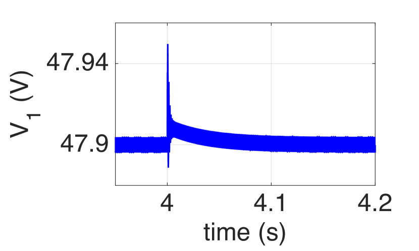
(a) Voltage at $PCC_{1}$.

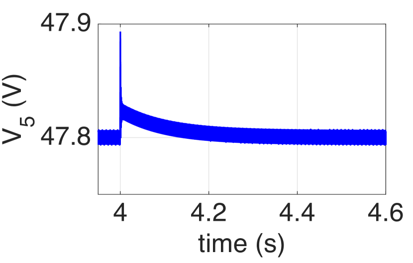
(b) Voltage at $PCC_{5}$.

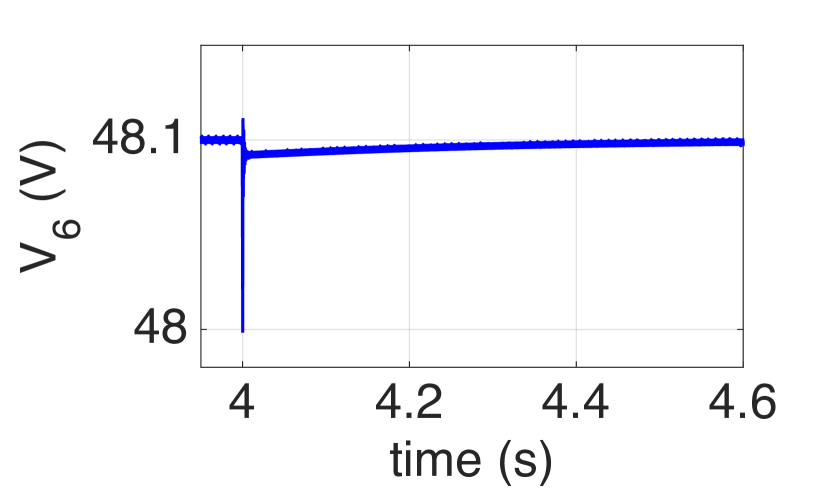
(c) Voltage at $PCC_{6}$.

Figure 3: Performance of PnP decentralized voltage controllers during the plug-in of DGU 6 at time $t=4$ s.

Robustness to unknown load changes

At $t=8$ s, the load of DGU 6 is decreased from $8\mbox{ }\Omega$ to $4\mbox{ }\Omega$. As shown in Figures 4(a)-4(b), right after $t=8$ the voltages at $PCC_{1}$ and $PCC_{5}$ slightly deviate from their references. However, these oscillations disappear after very short transients. A similar behavior can be noticed for the PCC voltage of DGU 6 (Figure 4(c)).

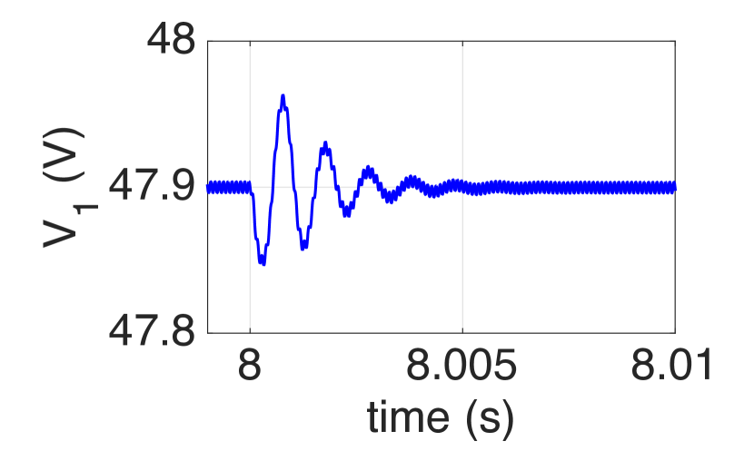
(a) Voltage at $PCC_{1}$.

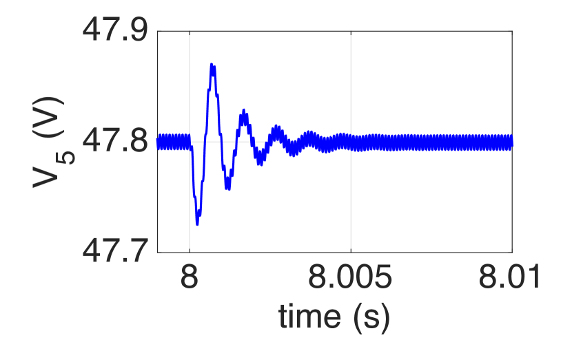
(b) Voltage at $PCC_{5}$.

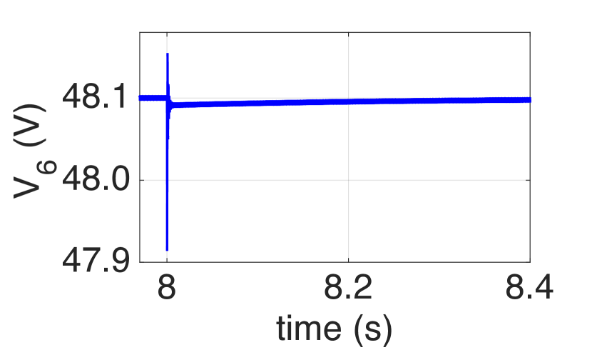
(c) Voltage at $PCC_{6}$.

Figure 4: Performance of PnP decentralized voltage controllers in terms of robustness to an abrupt change of load resistances at time $t=8$ s.

Unplugging of a DGU

At time $t=12s$ we perform the disconnection of ${\hat{\Sigma}}_{[3]}^{DGU}$ (see Figure 2). As described in Section 3.4, no controller update is required for the DGUs that were connected to it (i.e. DGUs 1 and 4). Figure 5 shows voltages at PCCs 1 and 4 around the unplugging event. Since controllers ${\mathcal{C}}_{[1]}$ and ${\mathcal{C}}_{[4]}$ do not need to be updated, subsystems ${\hat{\Sigma}}_{[j]}^{DGU}$, $j\in{\mathcal{N}}_{3}$, show deviations from their respective references which are smaller than those provided in [1].

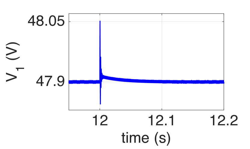
(a) Voltage at $PCC_{1}$.

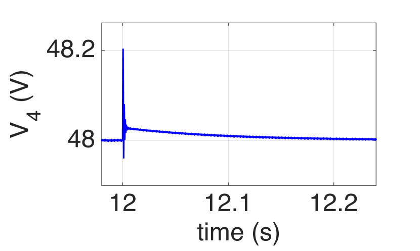
(b) Voltage at $PCC_{4}$.

Figure 5: Performance of PnP decentralized voltage controllers during the unplugging of DGU 3 at $t=12$ s.

5 Conclusions

In this paper, a totally decentralized scalable approach for voltage regulation in DC mG has been presented. Differently from the PnP design algorithm in [1, 7], the synthesis of local controllers does not require knowledge of power line parameters. Moreover, whenever the plug-in (resp. -out) of a DGU is required, its future (resp. previous) neighbors do not have to retune their local controller, thus considerably simplifying the PnP protocol while still guaranteeing the overall mG stability. Future research will focus on characterizing how performance of the closed-loop mG, depends on the topology of the electrical graph. We will also study how to couple the new PnP primary control layer with higher-level regulation schemes for achieving, e.g., current sharing.

Appendix A How interactions among DGUs can destabilize the mG

In this Appendix, we show why designing decentralized stabilizing controllers without taking into account Assumptions 1 and 2 (i.e. without counteracting the contribution of coupling terms on the total system energy computation) may lead to mG instability when DGUs are interconnected.

We consider two DGUs with dynamics

$${\hat{\Sigma}}_{[1]} :\left\{\begin{aligned} {\dot{\hat{x}}}_{[1]}(t)&=\hat{A}_{11}{\hat{x}}_{[1]}(t)+\hat{A}_{12}{\hat{x}}_{[2]}(t)+\hat{B}_{1}{u}_{[1]}(t)+\hat{M}_{1}{\hat{d}}_{[1]}(t)\\ {y}_{[1]}(t)&=\hat{C}_{1}{\hat{x}}_{[1]}(t)\end{aligned}\right.$$ (60)

$${\hat{\Sigma}}_{[2]} :\left\{\begin{aligned} {\dot{\hat{x}}}_{[2]}(t)&=\hat{A}_{22}{\hat{x}}_{[2]}(t)+\hat{A}_{21}{\hat{x}}_{[1]}(t)+\hat{B}_{2}{u}_{[2]}(t)+\hat{M}_{2}{\hat{d}}_{[2]}(t)\\ {y}_{[2]}(t)&=\hat{C}_{2}{\hat{x}}_{[2]}(t)\end{aligned}\right.$$

where ${\hat{x}}_{[i]}=[V_{i},I_{ti},v_{i}]^{T}$, ${u}_{[i]}=V_{ti}$, ${y}_{[i]}=V_{i}$, ${\hat{d}}_{[i]}=[I_{Li},V_{ref,i}]^{T}$, $i=1,2$, are, respectively, the state, the control input, the controlled variable and the exogenous input (see Section 2.2). Matrices in (60) have the same structure as in [1], i.e., since in this example ${\mathcal{N}}_{1}=\{2\}$ and ${\mathcal{N}}_{2}=\{1\}$, one has

$$A_{ii}=\begin{bmatrix}-\frac{1}{R_{ij}C_{ti}}&\frac{1}{C_{ti}}\\ -\frac{1}{L_{ti}}&-\frac{R_{ti}}{L_{ti}}\\ \end{bmatrix},\hskip 8.53581pti=1,2.$$ (61)

Electrical parameters, which are similar to those in [23], are reported in Table 1.

In the sequel, we separately analyze the impact of couplings on the mG stability when DGUs are locally stabilized via either Linear Quadratic Regulators (LQRs) or through pole placement design.

Linear Quadratic Regulators

We design decentralized controllers for each DGU assuming that they are dynamically decoupled, hence $\hat{A}_{12}=\hat{A}_{21}=0$. Since the state ${{\hat{x}}}_{[i]}$ is measured, we can design the following state-feedback decentralized controllers

$${u}_{[1]}(t) =K_{1}{\hat{x}}_{[1]}(t)$$ (62)

$${u}_{[2]}(t) =K_{2}{\hat{x}}_{[2]}(t)$$

where $K_{1}$ and $K_{2}$ are LQRs computed using the weights $Q_{1}={\mbox{diag}}(10^{-3},10^{-2},10^{3})$, $R_{1}=0.1$ and $Q_{2}={\mbox{diag}}(10^{-2},10^{-2},10^{4})$, $R_{2}=10^{-2}$, respectively. Control laws (62) guarantee that the closed-loop decoupled DGUs

$$\begin{bmatrix}{\dot{\hat{x}}}_{[1]}(t)\\ {\dot{\hat{x}}}_{[2]}(t)\end{bmatrix} =\begin{bmatrix}\hat{A}_{11}&0\\ 0&\hat{A}_{22}\\ \end{bmatrix}\begin{bmatrix}{\hat{x}}_{[1]}(t)\\ {\hat{x}}_{[2]}(t)\end{bmatrix}+\begin{bmatrix}\hat{B}_{1}K_{1}&0\\ 0&\hat{B}_{2}K_{2}\end{bmatrix}\begin{bmatrix}{\hat{x}}_{[1]}(t)\\ {\hat{x}}_{[2]}(t)\end{bmatrix}=$$ (63)

$$=\underbrace{\begin{bmatrix}\hat{A}_{11}+\hat{B}_{1}K_{1}&0\\ 0&\hat{A}_{22}+\hat{B}_{2}K_{2}\\ \end{bmatrix}}_{\mathbf{\hat{A}_{CL}^{D}}}\begin{bmatrix}{\hat{x}}_{[1]}(t)\\ {\hat{x}}_{[2]}(t)\end{bmatrix}$$

are asymptotically stable. Indeed, $\mathrm{eig}(\mathbf{\hat{A}_{CL}^{D}})=\mathrm{eig}(\hat{A}_{11}+\hat{B}_{1}K_{1})\text{ }\cup\text{ }\mathrm{eig}(\hat{A}_{22}+\hat{B}_{2}K_{2})$ is the set

$$\{-9.0629\cdot 10^{3},-0.0143\cdot 10^{3},-0.1945\cdot 10^{3}\}\cup\{-9.9717\cdot 10^{3},-0.0486\cdot 10^{3},-0.6064\cdot 10^{3}\}.$$

Considering coupling terms, the closed-loop system becomes

$$\begin{bmatrix}{\dot{\hat{x}}}_{[1]}(t)\\ {\dot{\hat{x}}}_{[2]}(t)\end{bmatrix} =\begin{bmatrix}\hat{A}_{11}&\hat{A}_{12}\\ \hat{A}_{21}&\hat{A}_{22}\\ \end{bmatrix}\begin{bmatrix}{\hat{x}}_{[1]}(t)\\ {\hat{x}}_{[2]}(t)\end{bmatrix}+\begin{bmatrix}\hat{B}_{1}K_{1}&0\\ 0&\hat{B}_{2}K_{2}\end{bmatrix}\begin{bmatrix}{\hat{x}}_{[1]}(t)\\ {\hat{x}}_{[2]}(t)\end{bmatrix}=$$ (64)

$$=\begin{bmatrix}{\dot{\hat{x}}}_{[1]}(t)\\ {\dot{\hat{x}}}_{[2]}(t)\end{bmatrix}\underbrace{\begin{bmatrix}\hat{A}_{11}+\hat{B}_{1}K_{1}&\hat{A}_{12}\\ \hat{A}_{21}&\hat{A}_{22}+\hat{B}_{1}K_{1}\\ \end{bmatrix}}_{\mathbf{\hat{A}_{CL}^{C}}}\begin{bmatrix}{\dot{\hat{x}}}_{[1]}(t)\\ {\dot{\hat{x}}}_{[2]}(t)\end{bmatrix}.$$

Since the controllers have been designed without taking into account interactions among DGUs, we cannot ensure that system (64) is asymptotically stable. In fact, for the proposed example, we have

$$\text{eig}(\mathbf{\hat{A}_{CL}^{C}})=\{-19077,\mathbf{20+560\mathrm{i}},\mathbf{20-560\mathrm{i}},-690,-161,-11\}.$$

Pole placement design

An alternative method for designing decentralized stabilizing controllers (62), is to assume again $\hat{A}_{12}=\hat{A}_{21}=0$ and place the closed-loop poles of subsystems ${\hat{\Sigma}}_{[1]}$ and ${\hat{\Sigma}}_{[2]}$ (i.e. the eigenvalues of $\mathbf{\hat{A}_{CL}^{D}}$) in the left half plane. In particular, since the pair $(\hat{A}_{ii},\hat{B}_{i})$ is controllable (see Proposition 2 in [1]), we can set

$$\text{eig}(\hat{A}_{11}+\hat{B}_{1}K_{1}) =\{-8.5190\cdot 10^{3},-530.4,-1.46\}$$ (65)

$$\text{eig}(\hat{A}_{22}+\hat{B}_{2}K_{2}) =\{-9.3734\cdot 10^{3},-571.9,-1.44\}$$

and derive gains $K_{1}$ and $K_{2}$ satisfying (65) by using the algorithm in [24]. Obviously, the obtained controllers stabilize the closed-loop decoupled subsystems (63). However, they cannot guarantee that the interconnection of DGUs 1 and 2 (i.e. system (64)) is asymptotically stable. Indeed, we get

$$\text{eig}(\mathbf{\hat{A}_{CL}^{C}})=\{-18803,\mathbf{23+2319\mathrm{i}},\mathbf{23-2319\mathrm{i}},-237,-0.16,-0.13\}.$$

Table 1: Electrical parameters of the mG with dynamics (60).

Converter parameters
DGU	$R_{t}$ $(\Omega)$	$L_{t}$ (mH)	$C_{t}$ (mF)
${\hat{\Sigma}}_{[1]}$	0.1	1.8	2.2
${\hat{\Sigma}}_{[2]}$	0.2	1.7	2
Transmission line parameters
$R_{12}$ $(\Omega)$		$L_{12}$ ($\mu$H)
0.05		1.8

Appendix B Feasibility of the LMI test

This Appendix summarizes the studies we performed in order to (i) evaluate the applicability of our line-independent control design procedure, and (ii) provide a proper comparison between the proposed approach and our previous work [1]. For both the analyses, LMIs have been solved in MatLab/Yalmip, using SeDuMi solver.

B.1 Line-independent design: conservativity of the plug-in test (58)

In order to better assess the applicability of the line-independent control design procedure (and to provide a guideline to the choice of $\bar{\sigma}$ in (12)), we performed the following extensive analysis. For $\bar{\sigma}=10$, we solved LMI (58) considering different values of the DGU’s converter parameters $(R_{t},L_{t},C_{t})$, and check when LMIs are infeasible.

Figure 6 shows combinations of these parameters for which the LMIs are feasible (blue circles), and infeasible (red stars). Although we used wide ranges for converter’s parameters, numerical results reveal that, for values typically found in the literature for low-voltage DC mGs (i.e. the points within the green box in Figure 6), LMIs are always feasible. This confirms the validity of the proposed control design methodology.

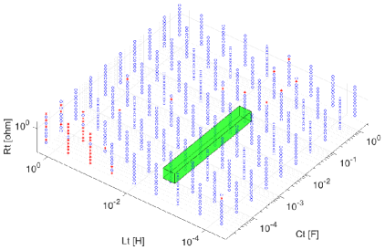
Figure 6: LMI results for combinations of $R_{t}$, $L_{t}$ and $C_{t}$. Blue circles indicate feasible LMIs while red stars correspond to infeasible ones. The green box encloses typical DGU parameters for low-voltage DC mGs.

B.2 Comparison with the line-dependent approach in [1]

In order to compare the proposed design methodology with the one in [1], we show the existence of a limit on the maximum number of subsystems which can be connected to the PCC of a given DGU (say DGU $i$), before obtaining the infeasibility of the $i$-th local line-dependent plug-in test (i.e. the LMI (25) in [1]).

We start by considering the interconnection of DGUs 1 and 2 at stage $k=1$ (see Figure 7(a)). Then, at each stage $k>1$, we solve the LMI (25) in [1] for DGU 1 (using $\eta=10^{-4}$), connecting one DGU at a time to $PCC_{1}$, thus creating the star topology shown in Figure 7(b). Electrical and optimization parameters used for this analysis are reported in Table 2.

Numerical results reveal that the feasibility test for DGU 1 fails when the plug-in of DGU 4 is requested. This is due to the fact that the design of each local controller depends on the parameters of power lines connecting the corresponding unit to its neighbors. On the other hand, in Appendix B.1 we have shown that, for $\bar{\sigma}=0$, the line-independent LMIs (58) are always feasible.

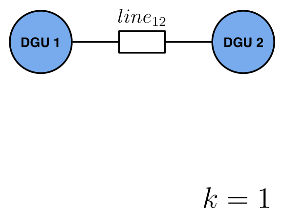
(a) Starting mG.

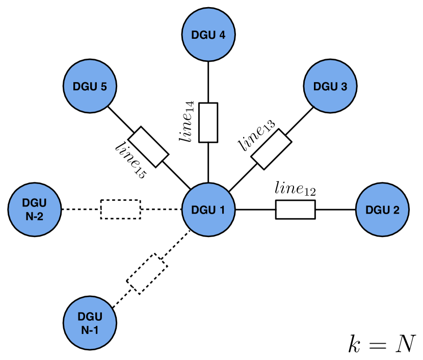
(b) Star-connected mG after $N$ stages.

Figure 7: Finding the maximum number of DGUs which can be connected $PCC_{1}$ before obtaining a plug-in request failure.

Table 2: Electrical and optimization parameters.

Converter parameters
DGU	$R_{t}$ $(\Omega)$	$L_{t}$ (mH)	$C_{t}$ (mF)
${\hat{\Sigma}}_{[1]}$	0.2	1.8	2.2
${\hat{\Sigma}}_{[2]}$	0.3	2	2.2
${\hat{\Sigma}}_{[3]}$	0.1	2.2	2.2
${\hat{\Sigma}}_{[4]}$	0.5	3	2.2
Transmission line parameters
Connected DGUs $(i,j)$		Resistance $R_{ij}(\Omega)$	Inductance $L_{ij}(\mu H)$
$(1,2)$		0.05	2.1
$(1,3)$		0.07	1.8
$(1,4)$		0.03	2.5
Optimization parameters
$\alpha_{1}$	$\alpha_{2}$		$\alpha_{3}$
$10^{-6}$	$10^{-2}$		$10^{-3}$

References

- [1] M. Tucci, S. Riverso, J. C. Vasquez, J. M. Guerrero, and G. Ferrari-Trecate, “A decentralized scalable approach to voltage control of dc islanded microgrids,” IEEE Transactions on Control Systems Technology, p. DOI: 10.1109/TCST.2016.2525001, 2015.
- [2] T. Dragičević, X. Lu, J. C. Vasquez, and J. M. Guerrero, “DC microgrids–part II: A review of power architectures, applications, and standardization issues,” IEEE Transactions on Power Electronics, vol. 31, no. 5, pp. 3528–3549, 2016.
- [3] T. Dragičević, X. Lu, J. Vasquez, and J. Guerrero, “DC microgrids–part I: A review of control strategies and stabilization techniques,” IEEE Transactions on Power Electronics, vol. 31, no. 7, pp. 4876–4891, 2016.
- [4] M. Andreasson, R. Wiget, D. Dimarogonas, K. Johansson, and G. Andersson, “Distributed primary frequency control through multi-terminal HVDC transmission systems,” in American Control Conference, 2015, pp. 5029–5034.
- [5] J. Zhao and F. Dörfler, “Distributed control and optimization in DC microgrids,” Automatica, vol. 61, pp. 18–26, 2015.
- [6] D. Zonetti, R. Ortega, and A. Benchaib, “A globally asymptotically stable decentralized PI controller for multi-terminal high-voltage DC transmission systems,” in European Control Conference, 2014, pp. 1397–1403.
- [7] M. Tucci, S. Riverso, J. C. Vasquez, J. M. Guerrero, and G. Ferrari-Trecate, “A decentralized scalable approach to voltage control of DC islanded microgrids,” Dipartimento di Ingegneria Industriale e dell’Informazione, Università degli Studi di Pavia, Pavia, Italy, Tech. Rep., 2015. [Online]. Available: arXiv:1405.2421
- [8] J. M. Guerrero, J. C. Vasquez, J. Matas, D. Vicuna, L. García, and M. Castilla, “Hierarchical control of droop-controlled AC and DC microgrids - A general approach toward standardization,” IEEE Transactions on Industrial Electronics, vol. 58, no. 1, pp. 158–172, 2011.
- [9] Q. Shafiee, T. Dragičević, J. C. Vasquez, and J. M. Guerrero, “Hierarchical Control for Multiple DC-Microgrids Clusters,” IEEE Transactions on Energy Conversion, vol. 29, no. 4, pp. 922–933, 2014.
- [10] S. Riverso, M. Farina, and G. Ferrari-Trecate, “Plug-and-Play Decentralized Model Predictive Control for Linear Systems,” IEEE Transactions on Automatic Control, vol. 58, no. 10, pp. 2608–2614, 2013.
- [11] ——, “Plug-and-Play Model Predictive Control based on robust control invariant sets,” Automatica, vol. 50, no. 8, pp. 2179–2186, 2014.
- [12] S. Bansal, M. Zeilinger, and C. Tomlin, “Plug-and-play model predictive control for electric vehicle charging and voltage control in smart grids,” in IEEE 53rd Conference on Decision and Control,, 2014, pp. 5894–5900.
- [13] G. Cezar, R. Rajagopal, and B. Zhang, “Stability of interconnected DC converters,” in 54th IEEE Conference on Decision and Control. IEEE, 2015, pp. 9––14.
- [14] M. Hamzeh, M. Ghafouri, H. Karimi, K. Sheshyekani, and J. Guerrero, “Power oscillations damping in dc microgrids,” IEEE Transactions on Energy Conversion, vol. 8969, no. To appear, 2016.
- [15] F. Dörfler and F. Bullo, “Kron reduction of graphs with applications to electrical networks,” IEEE Transactions on Circuits and Systems I: Regular Papers, vol. 60, no. 1, pp. 150–163, 2013.
- [16] H. K. Khalil, Nonlinear systems (3rd edition). Prentice Hall, 2001.
- [17] M. Babazadeh and H. Karimi, “A Robust Two-Degree-of-Freedom Control Strategy for an Islanded Microgrid,” IEEE Transactions on Power Delivery, vol. 28, no. 3, pp. 1339–1347, 2013.
- [18] V. Venkatasubramanian, H. Schattler, and J. Zaborszky, “Fast Time-Varying Phasor Analysis in the Balanced Three-Phase Large Electric Power System,” IEEE Transactions on Automatic Control, vol. 40, no. 11, pp. 1975–1982, 1995.
- [19] S. Skogestad and I. Postlethwaite, Multivariable feedback control: analysis and design. New York, NY, USA: John Wiley & Sons, 1996.
- [20] R. Grone, R. Merris, and V. S. Sunder, “The Laplacian spectrum of a graph,” SIAM Journal on Matrix Analysis and Applications, vol. 11, no. 2, pp. 218–238, 1990.
- [21] C. Godsil and G. Royle, “Algebraic graph theory, volume 207 of graduate texts in mathematics,” 2001.
- [22] S. Boyd, L. El Ghaoui, E. Feron, and V. Balakrishnan, Linear matrix inequalities in system and control theory. Philadelphia, Pennsylvania, USA: SIAM Studies in Applied Mathematics, vol. 15, 1994.
- [23] Q. Shafiee, T. Dragičević, J. C. Vasquez, and J. M. Guerrero, “Modeling, Stability Analysis and Active Stabilization of Multiple DC-Microgrid Clusters,” in Proceedings of the IEEE International Energy Conference (ENERGYCON), Dubrovnik, Croatia, May 13-16, 2014, pp. 1284–1290.
- [24] J. Kautsky, N. K. Nichols, and P. Van Dooren, “Robust pole assignment in linear state feedback,” International Journal of Control, vol. 41, no. 5, pp. 1129–1155, 1985.
- [25] M. Hamzeh, M. Ghafouri, H. Karimi, K. Sheshyekani, and J. M. Guerrero, “Power oscillations damping in DC microgrids,” IEEE Transactions on Energy Conversion, vol. 31, no. 3, pp. 970–980, Sept 2016.
- [26] T. Dragicevic, J. M. Guerrero, J. C. Vasquez, and D. Skrlec, “Supervisory control of an adaptive-droop regulated DC microgrid with battery management capability,” IEEE Transactions on Power Electronics, vol. 29, no. 2, pp. 695–706, Feb 2014.