Unveiling the nucleon tensor charge at Jefferson Lab: A study of the SoLID case

Abstract

Future experiments at the Jefferson Lab 12 GeV upgrade, in particular, the Solenoidal Large Intensity Device (SoLID), aim at a very precise data set in the region where the partonic structure of the nucleon is dominated by the valence quarks. One of the main goals is to constrain the quark transversity distributions. We apply recent theoretical advances of the global QCD extraction of the transversity distributions to study the impact of future experimental data from the SoLID experiments. Especially, we develop a simple strategy based on the Hessian matrix analysis that allows one to estimate the uncertainties of the transversity quark distributions and their tensor charges extracted from SoLID data simulation. We find that the SoLID measurements with the proton and the effective neutron targets can improve the precision of the $u$- and $d$-quark transversity distributions up to one order of magnitude in the range $0.05<x<0.6$.

1 Introduction

The nucleon tensor charge is a fundamental property of the nucleon and its determination is among the main goals of existing and future experimental facilities [1, 2, 3, 4, 5, 6, 7]. It also plays an important role in constraining new physics beyond the standard model [8, 9, 10] and has been an active subject of lattice QCD  [9, 11, 12, 13, 14, 15, 16, 17, 18, 19] and Dyson-Schwinger Equation (DSE) [20, 21] calculations. In terms of the partonic structure of the nucleon, the tensor charge, $\delta q$ for a particular quark type $q$, is constructed from the quark transversity distribution, $h_{1}(x,Q^{2})$, which is one of the three leading-twist quark distributions that describe completely spin-1/2 nucleon [1, 2, 3, 4, 5]:

$$\delta q\left(Q^{2}\right)\equiv\int_{0}^{1}dx\,\left(h_{1}^{q}(x,Q^{2})-h_{1}^{\bar{q}}(x,Q^{2})\right)\ .$$ (1)

It is extremely important to extend the experimental study of the quark transversity distribution to both large and small Bjorken $x$ to constrain the total tensor charge contributions. The Jefferson Lab 12 GeV program [6] is going to explore the region of relatively large-$x$ dominated by valence quarks while the planned Electron Ion Collider  [5, 7, 22] is going to extend the range to unexplored lower values of $x$, providing a possibility to study the anti-quark transversity distributions.

In this paper we analyze the impact of future proposed SoLID experiment at Jefferson Lab 12 GeV on the determination of tensor charge and transversity distributions for $u$- and $d$-quarks. Our studies are based on the QCD global fit of the available Semi-Inclusive Deep Inelastic Scattering (SIDIS) data and $e^{+}e^{-}$ annihilation into hadron pairs performed in Ref. [23] which we will refer as KPSY15. The current available experimental data suggests that anti-quark transversities are very small compared to $u$- and $d$-quark transversities. In this study we assumed that anti-quark transversities are negligible. Using the best fit of transversity distributions of Ref. [23] we simulated pseudodata for SoLID experiment and estimate the improvement of $u$- and $d$-quark transversity distributions with respect to our present knowledge. In order to perform a reliable estimate of improvement we develop a simple method based on Hessian error analysis described in Section 4.

This study also provides information on contribution of tensor charge from kinematical region of Jefferson Lab 12 GeV and will serve as a guide in planning future experiments.

2 Present status of extraction of transversity from experimental data

Transversity is a chiral odd quantity and thus in order to be measured in a physics process it should couple to another chiral odd distribution. There are several ways of accessing transversity. It can be studied in SIDIS process where it couples, for instance, to the Collins TMD fragmentation functions [24], and produces the so-called Collins asymmetries. Transversity can also couple to the dihadron interference fragmentation functions in SIDIS [25] and thus collinear transversity can be studied directly. Transversity can be studied in the Drell-Yan process in polarized hadron-hadron scattering [26, 27] where it couples either to anti-quark transversity or to the so-called the Boer-Mulders functions.

SIDIS experimental measurements have been made at HERMES  [28, 29], COMPASS  [30, 31, 32], and JLab HALL A [33] experiments. The BELLE, BABAR and the BESIII collaborations have studied the asymmetries in $e^{+}e^{-}$ annihilation into hadron pairs at the center of mass energy around $\sqrt{s}\simeq 10.6$ GeV [34, 35, 36], and $\sqrt{s}\simeq 3.6$ GeV [37], respectively.

The effort to extract transversity distributions and Collins fragmentation functions has been carried out extensively in the last few years [38, 39, 40, 41, 23]. QCD analysis of the data where transversity couples to the so-called dihadron interference fragmentation functions was performed in Ref. [42]. These results have demonstrated the powerful capability of the asymmetry measurements in constraining quark transversity distributions and hence the nucleon tensor charge in high energy scattering experiments. The first extraction of the transversity distributions and Collins fragmentation functions with TMD evolution was performed in Refs. [43, 23].

Collins asymmetries in SIDIS are generated by the convolution of the transversity function $h_{1}$ and Collins function $H_{1}^{\perp}$. The relevant contributions to the SIDIS cross-sections are

$$\frac{d^{5}\sigma(S_{\perp})}{dx_{B}dydzd^{2}P_{T}}=\sigma_{0}\Big{[}F_{UU}+\sin(\phi_{h}+\phi_{s})\,\frac{2(1-y)}{1+(1-y)^{2}}\,F_{UT}^{\sin\left(\phi_{h}+\phi_{s}\right)}+...\Big{]}\,,$$ (2)

where $\sigma_{0}=\frac{2\pi\alpha_{\rm em}^{2}}{Q^{2}}\frac{1+(1-y)^{2}}{y}$, and $\phi_{s}$ and $\phi_{h}$ are the azimuthal angles for the nucleon spin and the transverse momentum of the outgoing hadron with respect to the lepton plane, respectively. $F_{UU}$ and $F_{UT}^{\sin(\phi_{h}+\phi_{s})}$ are the unpolarized and transverse spin-dependent polarized structure functions respectively, and the ellipsis represents other polarized structure functions not relevant for this analysis. The polarized structure function $F_{UT}^{\sin\left(\phi_{h}+\phi_{s}\right)}$ contains the convolution of transversity distributions with the Collins  fragmentation functions, $h_{1}\otimes H_{1}^{\perp}$, and unpolarized structure function $F_{UU}$ is the convolution of the unpolarized TMD distributions and the unpolarized fragmentation functions, $f_{1}\otimes D_{1}$. The Collins asymmetry is defined as

$$A_{UT}^{\sin\left(\phi_{h}+\phi_{s}\right)}(x,y,z,P_{T})=\frac{2(1-y)}{1+(1-y)^{2}}\,\frac{F_{UT}^{\sin\left(\phi_{h}+\phi_{s}\right)}}{F_{UU}}\ .$$ (3)

Neglecting sea quark contributions, the structure function $F_{UT}^{\sin\left(\phi_{h}+\phi_{s}\right)}$ for the proton (P) and the neutron (N) targets can be written as:

$$F_{UT}^{\sin\left(\phi_{h}+\phi_{s}\right)}(P,\pi^{+}) =e_{u}^{2}h_{1}^{u}\otimes H_{1}^{\perp,fav}+e_{d}^{2}h_{1}^{d}\otimes H_{1}^{\perp,unf}\;,$$ (4)

$$F_{UT}^{\sin\left(\phi_{h}+\phi_{s}\right)}(P,\pi^{-}) =e_{u}^{2}h_{1}^{u}\otimes H_{1}^{\perp,unf}+e_{d}^{2}h_{1}^{d}\otimes H_{1}^{\perp,fav}\;,$$ (5)

$$F_{UT}^{\sin\left(\phi_{h}+\phi_{s}\right)}(N,\pi^{+}) =e_{u}^{2}h_{1}^{d}\otimes H_{1}^{\perp,fav}+e_{d}^{2}h_{1}^{u}\otimes H_{1}^{\perp,unf}\;,$$ (6)

$$F_{UT}^{\sin\left(\phi_{h}+\phi_{s}\right)}(N,\pi^{-}) =e_{u}^{2}h_{1}^{d}\otimes H_{1}^{\perp,unf}+e_{d}^{2}h_{1}^{u}\otimes H_{1}^{\perp,fav}\;.$$ (7)

Here $H_{1}^{\perp,fav}$ and $H_{1}^{\perp,unf}$, are the favored and the unfavored Collins fragmentation functions, respectively. In this context, favored refers to fragmentation of struck quarks of the same type as the constituent valence quarks of the produced pion while the unfavored being the opposite case. Previous global analysis [23, 40] have found that both the favored and unfavored Collins functions have approximately similar magnitude (with opposite signs). Therefore, since $e_{u}^{2}$ = 4$e_{d}^{2}$, the $u$-quark transversity is more constrained in the proton sample than $d$-quark transversity and the situation is reversed in the neutron case. One expects from these considerations that only the neutron target can help to reach the same relative impact on determination of $d$-quark transversity compared to improvement of $u$-quark transversity from the proton target data.

In the KPSY15 analysis the transversity distributions was parametrized as at the input scale $Q_{0}=\sqrt{2.4}$ GeV as

$$h_{1}^{q}(x,Q_{0})= N_{q}^{h}x^{a_{q}}(1-x)^{b_{q}}\frac{(a_{q}+b_{q})^{a_{q}+b_{q}}}{a_{q}^{a_{q}}b_{q}^{b_{q}}}\,\cdot\frac{1}{2}\left(f_{1}^{q}(x,Q_{0})+g_{1}^{q}(x,Q_{0})\right)\ ,$$ (8)

where $f_{1}^{q}$ and $g_{1}^{q}$ are the collinear unpolarized [44] and polarized [45] quark distributions for $q=u-$ and $d$-quark, respectively.

On the other hand, the twist-3 Collins fragmentation functions were parametrized in terms of the unpolarized fragmentation functions,

$$\hat{H}_{fav}^{(3)}(z,Q_{0}) =N_{u}^{c}z^{\alpha_{u}}(1-z)^{\beta_{u}}D_{\pi^{+}/u}(z,Q_{0})\ ,$$ (9)

$$\hat{H}_{unf}^{(3)}(z,Q_{0}) =N_{d}^{c}z^{\alpha_{d}}(1-z)^{\beta_{d}}D_{\pi^{+}/d}(z,Q_{0})\ ,$$ (10)

which correspond to the favored and unfavored Collins fragmentation functions, respectively. For $D_{\pi^{+}/q}$ we use the recent extraction from Ref. [46].

In summary, the analysis of KPSY15 used a total of 13 parameters in their global fit: $N_{u}^{h}$, $N_{d}^{h}$, $a_{u}$, $a_{d}$, $b_{u}$, $b_{d}$, $N_{u}^{c}$, $N_{d}^{c}$, $\alpha_{u}$, $\alpha_{d}$, $\beta_{d}$, $\beta_{u}$, $g_{c}$ (GeV²), where $g_{c}$ is a parameter to model the width of the Collins fragmentation function. The parameters are shown in Table 1.

$N_{u}^{h}$	=	$0.85\pm 0.09$	$a_{u}$	=	$0.69\pm 0.04$	$b_{u}$	=	$0.05\pm 0.04$
$N_{d}^{h}$	=	$-1.0\pm 0.13$	$a_{d}$	=	$1.79\pm 0.32$	$b_{d}$	=	$7.00\pm 2.65$
$N_{u}^{c}$	=	$-0.262\pm 0.025$	$\alpha_{u}$	=	$1.69\pm 0.01$	$\beta_{u}$	=	$0.00\pm 0.54$
$N_{d}^{c}$	=	$0.195\pm 0.007$	$\alpha_{d}$	=	$0.32\pm 0.04$	$\beta_{d}$	=	$0.00\pm 0.79$
$g_{c}$	=	$0.0236\pm 0.0007$	(GeV2)

Table 1: Fitted parameters of the transversity distributions for $u$- and $d$-quark, and Collins fragmentation functions. The table is from Ref. [23]

Since the existing experimental data have only probed the limited region $0.0065<x<0.35$, the following partial contribution to the tensor charge, neglecting anti-quark contributions, was defined [23]

$$\delta q^{[x_{\rm min},x_{\rm max}]}\left(Q^{2}\right)\equiv\int_{x_{\rm min}}^{x_{\rm max}}dx\,h_{1}^{q}(x,Q^{2})\ .$$ (11)

3 Simulated Data for SoLID

Several SIDIS experiments have been approved at Jefferson Lab 12 GeV to measure the asymmetries from proton and neutron targets with polarization in both the transverse and longitudinal directions. Among those, three Hall A experiments, E12-10-006 [47] (90 days), E12-11-007 [48] (35 days), and E12-11-108 [49] (120 days), plan to take data using the proposed high intensity and large acceptance device named SoLID [50, 51], and measure both the single-spin asymmetries (SSA) and double-spin asymmetries (DSA) on polarized $\mathrm{NH_{3}}$ (proton) and $\mathrm{{}^{3}He}$ (effective neutron) targets. These experiments can produce an extensive set of SIDIS data with very high accuracy and thus provide unique opportunity to study TMD structure functions in the valence quark region.

In these experiments, the electron beam energy will be set at two different values, 8.8 GeV and 11 GeV. The momentum of the detected electrons and hadrons can range from 1 GeV/c up to their maximum values. The SoLID configuration dedicated to the SIDIS measurements provides a full $2\pi$ coverage in azimuthal angle and a coverage of the polar angle from $8^{\circ}$ up to $24^{\circ}$. The polarized luminosities of the proton target and the $\mathrm{{}^{3}He}$ target are $10^{35}$ cm${}^{-2}\cdot$ s^-1 and $10^{36}$ cm${}^{-2}\cdot$ s^-1, respectively. The polarization and dilution factor of the proton ($\mathrm{{}^{3}He}$) target are 70% (60%) and 0.13 (0.3), respectively.

For the purpose of the present analysis, we simulate the Collins asymmetries using the KPSY15 parametrization at the kinematic settings presented in the proposals of these experiments  [47, 48, 49]. The high luminosity allows us to bin the data in four dimensions, e.g. $x$, $z$, $Q^{2}$, and $P_{T}$. The acceptance of the proposed SoLID measurements are summarized in Table 2. There are in total 1014 bins for $\mathrm{{}^{3}He}(e,e^{\prime})\pi^{+}$, 879 bins for $\mathrm{{}^{3}He}(e,e^{\prime})\pi^{-}$, 612 bins for $p(e,e^{\prime})\pi^{+}$, and 488 bins for $p(e,e^{\prime})\pi^{-}$, respectively. The number of events in each bin is calculated by integrating over the cross sections and acceptance of individual events in this bin, and then accounting for the detector efficiencies and the target related characteristics, such as the luminosity, target polarization, effective neutron polarization as well as the dilution factor. The average values of $x$, $z$, $Q^{2}$, and $P_{T}$ are recorded in each bin together with the statistical uncertainty.

We also estimate the overall systematic uncertainty related to the experimental measurement, such as the raw asymmetry, target polarization, detector resolution, nuclear effects, random coincidence, and radiative corrections. The final uncertainties of the simulated Collins asymmetries are given as statistical and systematic uncertainties added in quadrature.

Variable	Min	Max	Bin Size	Bins
$Q^{2}$	1.0 GeV2	8.0 GeV2	$\sim 1.0$ GeV2	6 bins
$z$	0.3	0.7	0.05	8 bins
$P_{T}$	0.0 GeV	1.6 GeV	0.2 GeV	$\leq$ 8 bins
$x$	0.05	0.6	NA	$\leq$ 8 bins

Table 2: Kinematic limits of SoLID. The bin-size for $P_{T}$ is doubled when number of total events $<5\times 10^{6}$, and the bin size in $x$ varies to keep number of events in one bin $\sim 10^{6}$. The actual bin size of the last bin with the center at $x=0.6$ will extend up to $x\sim 0.7$.

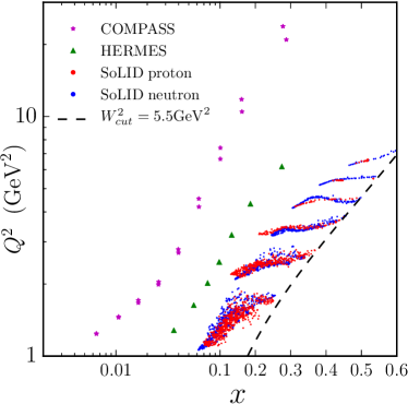
Figure 1: $x-Q^{2}$ kinematical plane of bins for SoLID data with HERMES [28, 29] and COMPASS [30, 31, 32] data sets.

The distribution of bins in $x-Q^{2}$ plane for SoLID and the comparison to HERMES [28, 29] and COMPASS [30, 31, 32], bins are presented in Fig. 1. The SoLID experiment plans to extend mainly into the larger $x$ region with $Q^{2}$ coverage comparable with HERMES. A direct comparison of the statistical precision of SoLID and the existing data is not possible due to different binning criteria between experiments, but an estimate of the level of precision can be given. For example, the average statistical precision of each bin for SoLID is about 1% consisting of more than 600 bins for $p(e,e^{\prime})\pi^{+}$ channel, compared to 37.1% (relative to the size of the asymmetry) for HERMES consisting of 7 bins in $x$ shown in Fig. 1 for the same channel. Note that SoLID implements $W^{2}$ cut at around 5.5 GeV². We leave the feasibility of implementing target mass corrections and usage of low $W$ region in the analysis of the experimental data for future developments of the theory and phenomenology.

4 Error estimation methodology from simulated data

In this section we describe the new method to estimate the impact of the future SoLID data to the transversity distribution of $u$- and $d$-quarks. Our method follows Bayesian statistics where the new information is added sequentially on top of the prior knowledge without requiring a combined analysis of the old data and the new data. We provide a simple strategy to quantify the impact of new measurements on the transversity distribution using the Hessian approach.

In general the information of the best fit parameters and their uncertainties is encoded in the likelihood function

$$\mathcal{L}(D|\bm{\alpha})\sim\exp\left(-\frac{1}{2}\chi^{2}(\bm{a},D)\right)$$ (12)

where $\bm{a}$ represents a vector of the model parameters and $D$ denotes collectively the experimental data points and their uncertainties . $\chi^{2}$ is the standard Chi-squared function defined as

$$\chi^{2}=\sum_{i}\left(\frac{D_{i}-T_{i}(\bm{a})}{\delta D_{i}}\right)^{2}\ ,$$ (13)

where $T_{i}(\bm{a})$ is the theoretical calculation for experimental measurement of $D_{i}$ and $\delta D_{i}$ is the experimental error of the measurement. The probability density of the parameters can be constructed from the likelihood function using the Bayes’ theorem:

$$\mathcal{P}(\bm{a}|D)\sim\mathcal{L}(D|\bm{a})~{}\pi(\bm{a})\ ,$$ (14)

where $\pi(\bm{a})$ is the prior distribution. Typically the latter is set to be normalized theta functions to remove unphysical regions in the parameter space. The expectation value and variance for an observable $\mathcal{O}$ (i.e. $h_{1}^{u,d},\delta u,\delta d$) can be estimated as

$$E[\mathcal{O}] =\int d^{n}a\ \mathcal{P}(\bm{a}|D)\ \mathcal{O}(\bm{a})\ ,$$

$$V[\mathcal{O}] =\int d^{n}a\ \mathcal{P}(\bm{a}|D)\ [\mathcal{O}(\bm{a})-E[\mathcal{O}]]^{2}\ .$$ (15)

In most of the situations the evaluation of the above integrals are not practical due to the large number of parameters needed in the model as well as numerical cost in evaluating $\mathcal{P}(\bm{a}|D)$ or equivalently the $\chi^{2}$ function. A traditional method to estimate Eq. (15) is the maximum likelihood (ML). First the parameters $\bm{a}_{0}$ that maximizes the likelihood (or minimized the $\chi^{2}$ function) is determined so that one can write

$$E[\mathcal{O}]\approx\mathcal{O}(\bm{a}_{0})\ .$$ (16)

A very simple method to estimate the variance is the Hessian approach [52, 53]. The idea is to compute the covariance matrix of the parameters using the Hessian of the $\chi^{2}$ function:

$$C_{i,j}^{-1}\approx H_{i,j}=\left.\frac{1}{2}\frac{\partial\chi^{2}(\bm{a},D)}{\partial a_{i}\partial a_{j}}\right|_{\bm{a}_{0}}\ .$$ (17)

From the eigen values $\lambda_{k}$ and their corresponding normalized eigen vectors $\bm{v}_{k}$ of the covariance matrix one can estimate the variance on $\mathcal{O}$ as

$$V[\mathcal{O}]=\frac{\Delta\chi^{2}}{4}\sum_{k}\left(\mathcal{O}(\bm{a}_{0}+\sqrt{\lambda_{k}}\bm{v}_{k})-\mathcal{O}(\bm{a}_{0}-\sqrt{\lambda_{k}}\bm{v}_{k})\right)^{2}.$$ (18)

The factor of $\Delta\chi^{2}$ (commonly known as the tolerance factor) is introduced in order to accommodate possible tensions among the data sets. In the ideal Gaussian statistics, $68\%$ CL corresponds to $\Delta\chi^{2}=1$. In the present analysis we use the value of $\Delta\chi^{2}=29.7$ quoted in the KPSY15 analysis. We stress however that our analysis focuses on the relative improvement after inclusion of the future SoLID data for which the tolerance factor drops out.

A simple Bayesian strategy to estimate the impact of the future measurements on the existing uncertainties is to update the covariance matrix. Since the only information provided is the projected statistical and systematic uncertainties, the expectation values (or equivalently $\bm{a}_{0}$) remain the same. To update the covariance matrix we note that the $\chi^{2}$ function is additive and one can write the new Hessian matrix as

$$H^{\rm New}_{i,j}=\left.\frac{1}{2}\frac{\partial\chi^{2}(\bm{a},D_{\rm old})}{\partial a_{i}\partial a_{j}}\right|_{\bm{a}_{0}}+\left.\frac{1}{2}\frac{\partial\chi^{2}(\bm{a},D_{\rm new})}{\partial a_{i}\partial a_{j}}\right|_{\bm{a}_{0}}\ ,$$ (19)

where $D_{old}$ is the data set used in a previous analysis (i.e. KPSY15) and the $D_{new}$ is the simulated data set for the future experiment. In our analysis only the covariance matrix from the KPSY15 analysis was provided. The new covariance matrix with the projected SoLID measurements was calculated as

$$C_{\rm New}^{-1}=H^{\rm New}_{i,j}=C_{\rm{\rm KPSY15}}^{-1}+\left.\frac{1}{2}\frac{\partial\chi^{2}(\bm{a},D_{\rm SoLID})}{\partial a_{i}\partial a_{j}}\right|_{\bm{a}_{0}}\ .$$ (20)

Using the new covariance matrix one can determine the impact of future data sets by estimating the uncertainties for the observables $\mathcal{O}$, such as transversity or tensor charges, using Eq. (18).

5 Tensor charge and transversity from SoLID

Our results for $u$- and $d$-quark transversity distributions at $Q^{2}=2.4$ GeV² are presented in Fig. 2 along with results from KPSY15. The uncertainties of KPSY15 are given as light shaded bands, while the projected errors after the SoLID data are taken into account are shown as dark shaded bands. To quantify the improvement of adding the future SoLID data, we show in the bottom plots of Fig. 2 the ratio of the estimated errors relative to the current errors. The results are shown using only the proton target data (left panels), the neutron data (central panels), and combination of the proton and the neutron data sets (right panels). In KPSY15 the uncertainty bands for transversity was calculated using the envelop method with a tolerance of $\Delta\chi^{2}=29.7$ which differs somehow from our Hessian error analysis. We stress that while the absolute error bands can differ depending on the error analysis, the ratio of the errors is independent of the error analysis.

One can see that, the proton target data improves $u$-quark transversity uncertainty (as can be seen from the left plot of the bottom panel of Fig. 2) while $d$-quark transversity improvement remains at a modest $\sim 60$% level. The effective neutron target data as expected allows for a much better improvement of $d$-quark transversity uncertainty (as can be seen from the central plot of the bottom panel of Fig. 2) and a relatively good improvement of $u$-quark (up to 80% reduction of errors) as well. It happens because of a higher statistics on the effective neutron target in comparison to the proton target. The right plot of the bottom panel of Fig. 2 shows that in the kinematical region of SoLID, $0.05<x<0.6$, the errors will be reduced by approximately 90%, i.e. one order of magnitude, for both $u$- and $d$-quark transversities if measurements are performed on both the proton and effective neutron targets.

Notice that the maximal improvements are attained in region covered by the SoLID data $0.05<x<0.6$ and the impact decreases outside of this region as expected. One may notice the “bump” around $x\simeq 0.2$ of the $d$-quark transversity in all three bottom plots. It appears to be an artifact of usage of Soffer positivity bound [54] in the parametrization of transversity for $u$- and $d$-quarks. Indeed, around $x\simeq 0.2$ the error corridor saturates the bound and it shows up as a “bump” in the ratio plot.

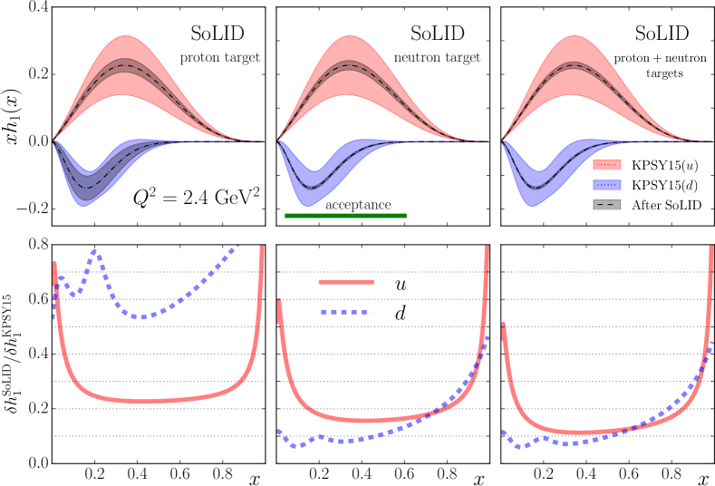
Figure 2: Upper panels: $u$-quark and $d$-quark transversity distributions at $Q^{2}=2.4$ (GeV²) as a function of $x$ with existing errors from KPSY15 (light shade area) and the estimated errors after the SoLID data (both statistical and systematical errors are included in quadrature) are taken into account. The acceptance region in $x$ of the SoLID experiment is indicated by the green horizontal line. Left plot: only the proton target data are taken into account, central plot: only the neutron target data are taken into account, right plot: combination of proton and neutron targets data are taken into account. Bottom panels: The ratio of the estimated errors and the current errors of transversity, $\delta h_{1}^{\rm SoLID}/\delta h_{1}^{\rm KPSY15}$, for $u$ (solid line) and $d$ (dashed line) quarks. Left plot: the proton target, central plot: the neutron target, right plot: combination of proton and neutron targets. The “bumps” around $x\simeq 0.2$ of the $d$-quark ratio plots are artifacts of usage of Soffer positivity bound [54] when parametrizing transversity.

Table 3: Table of tensor charges computed using Eq. (11). Tensor charges are calculated at $Q^{2}=2.4$ GeV² and $Q^{2}=10$ GeV² and in four regions of $x$ corresponding to the acceptance of SoLID, $0.05<x<0.6$; the full region, $0<x<1$; and the regions outside of acceptance, $0<x<0.05$, $0.6<x<1$. The errors are computed at 90% C.L. The isovector nulceon tensor charge $g_{T}$ is calculated using the full region $0<x<1$ and a truncated region $0.05<x<0.6$, see Eq. (21).

observable	$Q^{2}({\rm GeV^{2}})$	${\rm KPSY15}$	$\delta_{\rm KPSY15}$	$\delta_{\rm SoLID}$	$\delta_{\rm SoLID}/\delta_{\rm KPSY15}(\%)$
$\delta u^{[0,0.05]}$	2.4	0.046	0.010	0.005	49
$\delta u^{[0.05,0.6]}$	2.4	0.349	0.122	0.015	12
$\delta u^{[0.6,1]}$	2.4	0.018	0.007	0.001	14
$\delta u^{[0,1]}$	2.4	0.413	0.133	0.018	14
$\delta u^{[0,0.05]}$	10	0.051	0.011	0.005	46
$\delta u^{[0.05,0.6]}$	10	0.332	0.117	0.014	12
$\delta u^{[0.6,1]}$	10	0.0126	0.0048	0.0007	14
$\delta u^{[0,1]}$	10	0.395	0.128	0.018	14
$\delta d^{[0,0.05]}$	2.4	-0.029	0.028	0.003	10
$\delta d^{[0.05,0.6]}$	2.4	-0.200	0.073	0.006	9
$\delta d^{[0.6,1]}$	2.4	-0.00004	0.00009	0.00001	13
$\delta d^{[0,1]}$	2.4	-0.229	0.094	0.008	9
$\delta d^{[0,0.05]}$	10	-0.035	0.030	0.003	10
$\delta d^{[0.05,0.6]}$	10	-0.184	0.067	0.006	9
$\delta d^{[0.6,1]}$	10	-0.00002	0.00006	0.00001	14
$\delta d^{[0,1]}$	10	-0.219	0.090	0.008	9
$g_{T}^{(\rm truncated)}$	2.4	0.55	0.14	0.018	13
$g_{T}^{(\rm full)}$	2.4	0.64	0.15	0.021	14
$g_{T}^{(\rm truncated)}$	10	0.51	0.13	0.017	13
$g_{T}^{(\rm full)}$	10	0.61	0.14	0.020	14

The tensor charges can be calculated using Eq. (11) if one neglects sea-quark contributions. In Table 3 we present the estimated improvements for the truncated tensor charges at $Q^{2}=2.4$ GeV² and $Q^{2}=10$ GeV² separated into three kinematical regions of $x$: the region of SoLID acceptance ($0.05<x<0.6$) and the regions outside of SoLID coverage. For the region where SoLID has the maximum impact we find the improvement of about 90% (up to one order of magnitude) for both $u$- and $d$-quark tensor charges.

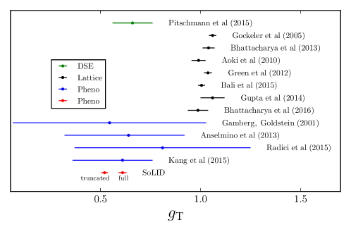
Figure 3: The isovector nucleon tensor charge $g_{T}$ after the pseudo-data of SoLID is taken into account is compared with result of Kang et al 2015 [23] at $Q^{2}=10$ GeV², result from Ref. [42] (Radici et al 2015) at 68% C.L. and $Q^{2}=4$ GeV², and result from Ref. [40] at 95% C.L. (Anselmino et al 2013) at $Q^{2}=0.8$ GeV², and Ref. [55] (Gamberg, Goldstein 2001) at $Q^{2}=1$ GeV². Other points are lattice computation at $Q^{2}=4$ GeV² of Bali et al Ref. [15], Gupta et al Ref. [16], Green et al Ref. [11], Aoki et al Ref. [18], Bhattacharya et al ref. [12, 13], Gockeler et al Ref. [19]. Pitschmann et al is DSE calculation Ref. [21] at $Q^{2}=4$ GeV². Two SoLID points are the truncated and full tensor charges from Eq. (21).

Finally we present our estimates for the precision of extraction of isovector nucleon tensor charge $g_{T}=\delta u-\delta d$, after the data of SoLID is taken into account:

$$g_{T}^{(\rm truncated)}=+0.55^{+0.018}_{-0.018}\ ,\quad\quad\quad g_{T}^{(\rm full)}=+0.64^{+0.021}_{-0.021}\ ,$$ (21)

at $Q^{2}=2.4$ GeV² where truncated means contribution from the region covered by the SoLID data $0.05<x<0.6$, and full is the contribution from $0<x<1$. See Table 3 for a detailed comparison. The precision of this result can be readily compared to precision of the lattice QCD calculations. As studied in Ref. [42], parametrizations of transversity that are substantially different in the region not covered by experimental data but similar in the region covered by the data lead to the growth of uncertainties of $g_{T}$ in the full kinematical region $0<x<1$. The relative improvement of the error, however, is less sensitive to the particular choice of parametrization especially in the region where data exists. With this in mind our result of the improvement of $g_{T}^{(\rm truncated)}$ is a more reliable estimate. As one can see from Eq. (21) and Fig. 3 we predict an order of magnitude improvement of the error. Future data from Electron Ion Collider will extend the region of the data and allow to explore low-x region.

In Fig. 3 we compare our result with extraction of Radici et al Ref. [42] at $Q^{2}=4$ GeV², Anselmino et al Ref. [40] at $Q^{2}=0.8$ GeV²; Gamberg, Goldstein 2001 Ref. [55] at $Q^{2}=1$ GeV². Our result is also compared to a series of lattice computations, at $Q^{2}=4$ GeV² of Bali et al Ref. [15], Gupta et al Ref. [16], Green et al Ref. [11], Aoki et al Ref. [18], Bhattacharya et al Refs. [12, 13], Gockeler et al Ref. [19]. Pitschmann et al [21] is a DSE calculation at $Q^{2}=4$ GeV². The value of $g_{T}$ extracted from the data may influence searches beyond the standard model [8, 9, 10].

6 Summary and Conclusions

We have studied impact of future SoLID data on both the proton and the effective neutron targets on extraction of transversity for $u$- and $d$-quarks and tensor charge of the nucleon. A new method based on Hessian error analysis was developed in order to estimate the impact of future new data sets on TMD distributions. Based on the global QCD analysis with TMD evolution of the current data of Ref. [23] we estimated that the combination of both the proton and the effective neutron targets is essential for the appropriate extraction of tensor charge. As one can clearly see in Fig. 2 we predict a balanced improvement in the precision of extraction for both $u$- and $d$-quarks up to one order of magnitude in the range $0.05<x<0.6$ with such a combination of measurements.

We would like to emphasize that it is also important to investigate other possible contributions to asymmetries that may influence extraction of the quark transversity distributions from the experimental data. One particular example is the higher-twist contributions, which can be thoroughly studied when the future data are available from Jefferson Lab 12 GeV upgrade, including both spin-averaged and spin-dependent cross section measurements. In addition, with the wide kinematic coverage in $Q^{2}$, the planed Electron Ion Collider will provide valuable information on higher twist contributions as well.

Under assumptions of Ref. [23] we also predict an impressive improvement in the extraction of tensor charge as can be seen in Table 3 in the presence of SoLID measurements. It appears that the acceptance region of SoLID will reveal most of contribution from $u$ and $d$ quarks to the tensor charge of the nucleon. The contribution from the region of high-$x$ not covered by SoLID ($x>0.6$) appear to be small for both $u$ and $d$ quarks, see Table 3. The same is true for the contribution from low-$x$ region, ($x<0.05$). The contribution to the tensor charge from anti-quarks at low-$x$ region was omitted in the present analysis. We leave for future the study of the impact of the Electron Ion Collider on the sea-quark transversity distributions.

The precision at which isovector tensor charge $g_{T}$ can be extracted from the SoLID data will be comparable to the precision of lattice QCD calculates, as can be seen from Fig. 3, and will provide a unique opportunity for searches beyond the standard model. Our results demonstrate the powerful capabilities of future measurements of SoLID apparatus at Jefferson Lab 12 GeV Upgrade.

References

References

- [1] J. P. Ralston, D. E. Soper, Production of dimuons from high-energy polarized proton- proton collisions, Nucl. Phys. B152 (1979) 109.
- [2] R. L. Jaffe, X. Ji, Chiral odd parton distributions and polarized Drell-Yan, Phys. Rev. Lett. 67 (1991) 552–555.
- [3] J. L. Cortes, B. Pire, J. P. Ralston, Measuring the transverse polarization of quarks in the proton, Z. Phys. C55 (1992) 409–416. doi:10.1007/BF01565099.
- [4] V. Barone, A. Drago, P. G. Ratcliffe, Transverse polarisation of quarks in hadrons, Phys. Rept. 359 (2002) 1–168. arXiv:hep-ph/0104283.
- [5] D. Boer, M. Diehl, R. Milner, R. Venugopalan, W. Vogelsang, et al., Gluons and the quark sea at high energies: Distributions, polarization, tomographyarXiv:1108.1713.
- [6] J. Dudek, R. Ent, R. Essig, K. Kumar, C. Meyer, et al., Physics Opportunities with the 12 GeV Upgrade at Jefferson Lab, Eur.Phys.J. A48 (2012) 187. arXiv:1208.1244, doi:10.1140/epja/i2012-12187-1.
- [7] A. Accardi, J. Albacete, M. Anselmino, N. Armesto, E. Aschenauer, et al., Electron Ion Collider: The Next QCD Frontier - Understanding the glue that binds us allarXiv:1212.1701.
- [8] M. Cirelli, E. Del Nobile, P. Panci, Tools for model-independent bounds in direct dark matter searches, JCAP 1310 (2013) 019. arXiv:1307.5955, doi:10.1088/1475-7516/2013/10/019.
- [9] T. Bhattacharya, V. Cirigliano, S. D. Cohen, A. Filipuzzi, M. Gonzalez-Alonso, et al., Probing Novel Scalar and Tensor Interactions from (Ultra)Cold Neutrons to the LHC, Phys.Rev. D85 (2012) 054512. arXiv:1110.6448, doi:10.1103/PhysRevD.85.054512.
- [10] A. Courtoy, S. Bae ler, M. Gonz lez-Alonso, S. Liuti, Beyond-Standard-Model Tensor Interaction and Hadron Phenomenology, Phys. Rev. Lett. 115 (2015) 162001. arXiv:1503.06814, doi:10.1103/PhysRevLett.115.162001.
- [11] J. Green, J. Negele, A. Pochinsky, S. Syritsyn, M. Engelhardt, et al., Nucleon Scalar and Tensor Charges from Lattice QCD with Light Wilson Quarks, Phys.Rev. D86 (2012) 114509. arXiv:1206.4527, doi:10.1103/PhysRevD.86.114509.
- [12] T. Bhattacharya, S. D. Cohen, R. Gupta, A. Joseph, H.-W. Lin, et al., Nucleon Charges and Electromagnetic Form Factors from 2+1+1-Flavor Lattice QCD, Phys.Rev. D89 (9) (2014) 094502. arXiv:1306.5435, doi:10.1103/PhysRevD.89.094502.
- [13] T. Bhattacharya, V. Cirigliano, S. Cohen, R. Gupta, H.-W. Lin, B. Yoon, Axial, Scalar and Tensor Charges of the Nucleon from 2+1+1-flavor Lattice QCDarXiv:1606.07049.
- [14] J.-W. Chen, S. D. Cohen, X. Ji, H.-W. Lin, J.-H. Zhang, Nucleon Helicity and Transversity Parton Distributions from Lattice QCD, Nucl. Phys. B911 (2016) 246–273. arXiv:1603.06664, doi:10.1016/j.nuclphysb.2016.07.033.
- [15] G. S. Bali, S. Collins, B. Gl ssle, M. G ckeler, J. Najjar, et al., Nucleon isovector couplings from lattice QCD, Phys.Rev. D91 (5) (2015) 054501. arXiv:1412.7336, doi:10.1103/PhysRevD.91.054501.
- [16] R. Gupta, T. Bhattacharya, A. Joseph, H.-W. Lin, B. Yoon, Precision calculations of nucleon charges , , , PoS Lattice2014 (2014) 152. arXiv:1501.07639.
- [17] N. Yamanaka, H. Ohki, S. Hashimoto, T. Kaneko, Nucleon axial and tensor charges with dynamical overlap quarks, PoS LATTICE2015 (2016) 121. arXiv:1511.04589.
- [18] Y. Aoki, T. Blum, H.-W. Lin, S. Ohta, S. Sasaki, et al., Nucleon isovector structure functions in (2+1)-flavor QCD with domain wall fermions, Phys.Rev. D82 (2010) 014501. arXiv:1003.3387, doi:10.1103/PhysRevD.82.014501.
- [19] M. Gockeler, et al., Quark helicity flip generalized parton distributions from two-flavor lattice QCD, Phys.Lett. B627 (2005) 113–123. arXiv:hep-lat/0507001, doi:10.1016/j.physletb.2005.09.002.
- [20] N. Yamanaka, T. M. Doi, S. Imai, H. Suganuma, Quark tensor charge and electric dipole moment within the Schwinger-Dyson formalism, Phys. Rev. D88 (2013) 074036. arXiv:1307.4208, doi:10.1103/PhysRevD.88.074036.
- [21] M. Pitschmann, C.-Y. Seng, C. D. Roberts, S. M. Schmidt, Nucleon tensor charges and electric dipole moments, Phys.Rev. D91 (7) (2015) 074004. arXiv:1411.2052, doi:10.1103/PhysRevD.91.074004.
-
[22]
E.-C. Aschenauer, et al.,
Pre-Town
Meeting on Spin Physics at an Electron-Ion Collider, 2014.
arXiv:1410.8831.
URL http://inspirehep.net/record/1325551/files/arXiv:1410.8831.pdf - [23] Z.-B. Kang, A. Prokudin, P. Sun, F. Yuan, Extraction of Quark Transversity Distribution and Collins Fragmentation Functions with QCD Evolution, Phys. Rev. D93 (1) (2016) 014009. arXiv:1505.05589, doi:10.1103/PhysRevD.93.014009.
- [24] J. C. Collins, Fragmentation of transversely polarized quarks probed in transverse momentum distributions, Nucl.Phys. B396 (1993) 161–182. arXiv:hep-ph/9208213, doi:10.1016/0550-3213(93)90262-N.
- [25] J. C. Collins, S. F. Heppelmann, G. A. Ladinsky, Measuring transversity densities in singly polarized hadron hadron and lepton - hadron collisions, Nucl. Phys. B420 (1994) 565–582. arXiv:hep-ph/9305309, doi:10.1016/0550-3213(94)90078-7.
- [26] V. Barone, et al., Antiproton-proton scattering experiments with polarizationarXiv:hep-ex/0505054.
- [27] E.-C. Aschenauer, et al., The RHIC SPIN Program: Achievements and Future OpportunitiesarXiv:1501.01220.
- [28] A. Airapetian, et al., Single-spin asymmetries in semi-inclusive deep-inelastic scattering on a transversely polarized hydrogen target, Phys. Rev. Lett. 94 (2005) 012002. arXiv:hep-ex/0408013.
- [29] A. Airapetian, et al., Effects of transversity in deep-inelastic scattering by polarized protons, Phys. Lett. B693 (2010) 11–16. arXiv:1006.4221, doi:10.1016/j.physletb.2010.08.012.
- [30] M. Alekseev, et al., Collins and Sivers asymmetries for pions and kaons in muon-deuteron DIS, Phys. Lett. B673 (2009) 127–135. arXiv:0802.2160, doi:10.1016/j.physletb.2009.01.060.
- [31] C. Adolph, et al., Experimental investigation of transverse spin asymmetries in muon-p SIDIS processes: Collins asymmetries, Phys.Lett. B717 (2012) 376–382. arXiv:1205.5121, doi:10.1016/j.physletb.2012.09.055.
- [32] C. Adolph, et al., Collins and Sivers asymmetries in muonproduction of pions and kaons off transversely polarised protons, Phys. Lett. B744 (2015) 250–259. arXiv:1408.4405, doi:10.1016/j.physletb.2015.03.056.
- [33] X. Qian, et al., Single Spin Asymmetries in Charged Pion Production from Semi-Inclusive Deep Inelastic Scattering on a Transversely Polarized 3He Target, Phys.Rev.Lett. 107 (2011) 072003. arXiv:1106.0363, doi:10.1103/PhysRevLett.107.072003.
- [34] K. Abe, et al., Measurement of azimuthal asymmetries in inclusive production of hadron pairs in e+ e- annihilation at Belle, Phys. Rev. Lett. 96 (2006) 232002. arXiv:hep-ex/0507063, doi:10.1103/PhysRevLett.96.232002.
- [35] R. Seidl, et al., Measurement of Azimuthal Asymmetries in Inclusive Production of Hadron Pairs in e+e- Annihilation at GeV, Phys. Rev. D78 (2008) 032011. arXiv:0805.2975, doi:10.1103/PhysRevD.78.032011.
- [36] I. Garzia, Measurement of Collins asymmetries in inclusive production of pion pairs in collisions at BABAR, PoS ICHEP2012 (2013) 272. arXiv:1211.5293.
- [37] M. Ablikim, et al., Measurement of azimuthal asymmetries in inclusive charged dipion production in annihilations at = 3.65 GeVarXiv:1507.06824.
- [38] M. Anselmino, et al., Transversity and Collins functions from SIDIS and e+ e- data, Phys. Rev. D75 (2007) 054032. arXiv:hep-ph/0701006.
- [39] M. Anselmino, M. Boglione, U. D’Alesio, A. Kotzinian, F. Murgia, A. Prokudin, S. Melis, Update on transversity and Collins functions from SIDIS and e+ e- data, Nucl. Phys. Proc. Suppl. 191 (2009) 98–107. arXiv:0812.4366, doi:10.1016/j.nuclphysbps.2009.03.117.
- [40] M. Anselmino, M. Boglione, U. D’Alesio, S. Melis, F. Murgia, et al., Simultaneous extraction of transversity and Collins functions from new SIDIS and e+e- data, Phys.Rev. D87 (2013) 094019. arXiv:1303.3822, doi:10.1103/PhysRevD.87.094019.
- [41] M. Anselmino, M. Boglione, U. D’Alesio, J. O. Gonzalez Hernandez, S. Melis, F. Murgia, A. Prokudin, Collins functions for pions from SIDIS and new data: a first glance at their transverse momentum dependence, Phys. Rev. D92 (11) (2015) 114023. arXiv:1510.05389, doi:10.1103/PhysRevD.92.114023.
- [42] M. Radici, A. Courtoy, A. Bacchetta, M. Guagnelli, Improved extraction of valence transversity distributions from inclusive dihadron production, JHEP 05 (2015) 123. arXiv:1503.03495, doi:10.1007/JHEP05(2015)123.
- [43] Z.-B. Kang, A. Prokudin, P. Sun, F. Yuan, Nucleon tensor charge from Collins azimuthal asymmetry measurements, Phys.Rev. D91 (7) (2015) 071501. arXiv:1410.4877, doi:10.1103/PhysRevD.91.071501.
- [44] H.-L. Lai, M. Guzzi, J. Huston, Z. Li, P. M. Nadolsky, et al., New parton distributions for collider physics, Phys.Rev. D82 (2010) 074024. arXiv:1007.2241, doi:10.1103/PhysRevD.82.074024.
- [45] D. de Florian, R. Sassot, M. Stratmann, W. Vogelsang, Extraction of Spin-Dependent Parton Densities and Their Uncertainties, Phys.Rev. D80 (2009) 034030. arXiv:0904.3821, doi:10.1103/PhysRevD.80.034030.
- [46] D. de Florian, R. Sassot, M. Epele, R. J. Hernández-Pinto, M. Stratmann, Parton-to-Pion Fragmentation Reloaded, Phys.Rev. D91 (1) (2015) 014035. arXiv:1410.6027, doi:10.1103/PhysRevD.91.014035.
-
[47]
E12-10-006,
SIDIS
with Transversely Polarized 3He Target using SoLID.
URL http://hallaweb.jlab.org/collab/PAC/PAC35/PR-10-006-SoLID-Transversity.pdf -
[48]
E12-11-007,
SIDIS
with Longitudinally Polarized 3He Target using SoLID.
URL http://www.jlab.org/exp_prog/PACpage/PAC37/proposals/Proposals/New%20Proposals/PR-11-007.pdf -
[49]
E12-11-108,
SIDIS with
Polarized Proton Target using SoLID.
URL https://www.jlab.org/exp_prog/proposals/11/PR12-11-108.pdf -
[50]
SoLID-Collaboration,
Solenoidal
Large Intensity Device (SoLID) Preliminary Conceptual Design Report.
URL http://hallaweb.jlab.org/12GeV/SoLID/download/doc/solid_precdr.pdf - [51] J. P. Chen, H. Gao, T. K. Hemmick, Z. E. Meziani, P. A. Souder, A White Paper on SoLID (Solenoidal Large Intensity Device)arXiv:1409.7741.
- [52] D. Stump, J. Pumplin, R. Brock, D. Casey, J. Huston, J. Kalk, H. L. Lai, W. K. Tung, Uncertainties of predictions from parton distribution functions. 1. The Lagrange multiplier method, Phys. Rev. D65 (2001) 014012. arXiv:hep-ph/0101051, doi:10.1103/PhysRevD.65.014012.
- [53] J. Pumplin, D. Stump, R. Brock, D. Casey, J. Huston, J. Kalk, H. L. Lai, W. K. Tung, Uncertainties of predictions from parton distribution functions. 2. The Hessian method, Phys. Rev. D65 (2001) 014013. arXiv:hep-ph/0101032, doi:10.1103/PhysRevD.65.014013.
- [54] J. Soffer, Positivity constraints for spin dependent parton distributions, Phys. Rev. Lett. 74 (1995) 1292–1294. arXiv:hep-ph/9409254, doi:10.1103/PhysRevLett.74.1292.
- [55] L. P. Gamberg, G. R. Goldstein, Flavor spin symmetry estimate of the nucleon tensor charge, Phys. Rev. Lett. 87 (2001) 242001. arXiv:hep-ph/0107176, doi:10.1103/PhysRevLett.87.242001.