On the Performance Analysis of Underlay Cognitive Radio Systems: A Deployment Perspective

Abstract

We study the performance of cognitive Underlay System (US) that employ power control mechanism at the Secondary Transmitter (ST) from a deployment perspective. Existing baseline models considered for performance analysis either assume the knowledge of involved channels at the ST or retrieve this information by means of a band manager or a feedback channel, however, such situations rarely exist in practice. Motivated by this fact, we propose a novel approach that incorporates estimation of the involved channels at the ST, in order to characterize the performance of the US in terms of interference power received at the primary receiver and throughput at the secondary receiver (or secondary throughput). Moreover, we apply an outage constraint that captures the impact of imperfect channel knowledge, particularly on the uncertain interference. Besides this, we employ a transmit power constraint at the ST to classify the operation of the US in terms of an interference-limited regime and a power-limited regime. In addition, we characterize the expressions of the uncertain interference and the secondary throughput for the case where the involved channels encounter Nakagami-$m$ fading. Finally, we investigate a fundamental tradeoff between the estimation time and the secondary throughput depicting an optimized performance of the US.

I Introduction

Cognitive Radio (CR) communications is considered as one of the viable solutions that addresses the problem of spectrum scarcity of future wireless networks. Secondary access to the licensed spectrum can be broadly categorized into different CR paradigms, namely, interweave, underlay and overlay systems [2]. Among these, underlay and interweave systems are largely associated with the techniques that are applicable at the physical layer and therefore can be considered feasible for hardware deployment. The interweave systems employ spectrum sensing to detect the presence of primary user signals while avoiding harmful interference to the primary system. On the other hand, an Underlay System (US) exploits the interference tolerance capability of the primary systems that allows the secondary users to transmit even in the presence of the primary users. To accomplish this, the US employs techniques such as power control to maintain the interference (power) received at the Primary Receiver (PR) below a specified level, defined as Interference Threshold (IT) [3]. In this paper, we focus on the performance characterization of the US that employs power control at the Secondary Transmitter (ST).

I-A Motivation and Related Work

In order to enable shared access to the licensed spectrum, it is essential to characterize the performance of a CR system in reference to the primary and the secondary systems. With regard to the primary system, the performance of a US is characterized in terms of interference received at the PR, which arises due to concurrent data transmission over the same channel by the secondary system. Recently, power control at the ST has emerged as an effective way of regulating the interference induced by the ST. However, the power control primarily requires the knowledge of the primary interference channel between the ST and the PR at the ST. The preliminary investigations [3, 4, 5, 6, 7], considered for the performance evaluation of the US, assume this knowledge to be perfectly known at the ST. Such situations rarely exist in practical implementations. In order to address this, the performance analysis based on imperfect channel knowledge has been dealt extensively in [8, 9, 10, 11, 12, 13, 14, 15, 16, 17, 18].

It is worth noticing that the majority of these works [8, 11, 10] in reference to the imperfect channel knowledge consider that the channel’s knowledge at the ST is obtained from a band manager, an approach proposed in [19]. Whereas [13, 9] rely on the presence of a feedback link from the PR to the ST [20]. The fact is, the feasibility of the band manager or the feedback link across two different systems is unrealistic from a practical standpoint. In addition, due to latency, the channel knowledge obtained while implementing these approaches may be outdated, as considered in [9, 10, 11, 13]. Besides, for the existence of the feedback link, the demodulation of the secondary user signals at the PR and a resource (time) allocation explicitly for communicating the channel knowledge impose an additional overhead for the primary system. These issues render the hardware implementation of the US in reference to the aforementioned approaches challenging. In contrast to these approaches, we propose a novel strategy, according to which the channel estimation is employed directly at the secondary system. Thus, by avoiding the realization of the band manager or the feedback link and the issues related to it, this paper outlines the key aspects that facilitate the hardware deployment of the US.

Along with the performance of the primary system, the achievable data rate at the Secondary Receiver (SR) for the link between the ST and the SR contributes significantly to the overall performance of the US [8, 7, 9, 15, 14, 11, 13]. As a matter of fact, the knowledge of the data rate at the ST can be utilized for guaranteeing a certain quality of service, which enables us to visualize potential applications or prominent use cases for the CR system. In order to characterize the data rate, the ST (along with the primary interference channel, which is associated with power control mechanism) requires the knowledge of access channel between the ST and the SR, and secondary interference channel between the Primary Transmitter (PT) and the SR. Despite these facts, the performance characterization of the US’s data rate in reference to the estimation of the access and the secondary interference channels has not been considered in [8, 9, 10, 11, 13, 14] or only marginally in [12, 15, 16].

From a deployment perspective, it is worthy to understand that the interference channels are representative of the channels that exist between different (primary and secondary) systems. This signifies that in order to carry out channel estimation based on the conventional techniques such as pilot-based channel estimation, which is mainly employed in the previous works, a preliminary processing of the primary user signal is necessary. The existence of multiple wireless standards and their complexity forbid the deployment of a dedicated circuitry corresponding to each primary user signals [21]. In this regard, in order to facilitate hardware deployment of the US, it is necessary to select the estimation techniques such that the complexity and the versatility (to the unknown primary user signals) requirements are satisfied. In this paper, similar to [22], we address this critical problem by employing a received power-based estimation at the ST and the SR for the interference channels. In contrast to the interweave scenario considered in [22], we investigate an underlay scenario herein. Recently, a successful deployment of the received power-based channel estimation at the ST in context to the US has been studied in [23].

In addition, [8, 9, 10, 11, 12, 13, 14, 15, 16, 17] consider that the PR employs pilot-based channel estimation for the channel PR-ST, which is possible only if the PR is willing: (i) to allocate time resources, (ii) to assign a dedicated circuitry for demodulating the secondary user signals and (iii) to establish a feedback link to the ST, thereby challenging the hardware implementation of the US. In contrast, for the proposed received power-based estimation, a certain time needs to be allocated by the secondary user for channel estimation that affects the secondary throughput. Since the aspect concerning the time allocation for the channel estimation has not been taken into account in any of the previous investigations related to the cognitive US [8, 9, 10, 11, 12, 13, 14, 15, 16, 17], the performance of the US in terms of the secondary throughput is overestimated. Moreover, the imperfect knowledge of the primary interference channel leads to an uncertainty in the interference at the PR, which in certain cases may exceed the IT. Under such conditions, the conventional constraint imposed in [3, 4, 7, 6] is strictly violated. As a result, this uncertain interference originated from imperfect channel knowledge may seriously degrade the performance of the primary systems. In order to tackle this issue, we propose to employ an outage constraint that regulates the uncertain interference caused at the PR.

Besides, through analysis (performed later in Section III), it is revealed that the uncertain interference is associated with the estimation time and the controlled power. In this context, the estimation time is indirectly associated with the secondary throughput through the controlled power, signifying the influence of the imperfect channel knowledge. On the other side, the time allocation directly affects the secondary throughput. In this paper, we examine this relationship between the estimation time and the secondary throughput while constraining the uncertain interference below a desired level. Although the previous studies have considered channel estimation, the effect of the imperfect channel knowledge in terms of the time allocation and the uncertain interference in context to the US is still underdeveloped.

I-B Contributions

In this paper, we provide the following contributions:

I-B1 Analytical Framework

The main contribution of this paper is to derive an analytical framework for underlay CR systems that employ a power control mechanism and incorporate the estimation of the following interacting channels: (i) primary interference channel between the ST and the PR, (ii) secondary interference channel between the PT and the SR, and (iii) access channel between the ST and the SR. In contrast to the existing works that demand the presence of a band manager or a feedback link in order to retrieve channel knowledge, we propose to employ channel estimation at the secondary system. In order to facilitate the deployment of the US, we propose to employ received power-based channel estimation, specially for the interference channels so that low complexity and versatility requirements to estimate primary user signals is accomplished. Clearly, the channel estimation is detrimental (in terms of the time allocation and the uncertain interference) to the performance of the US, leading to performance degradation. By comparing its performance with the ideal scenario (with perfect channel knowledge), we study the performance degradation caused due to the imperfect channel knowledge.

Besides, we characterize the variations due to the imperfect channel knowledge in the performance parameters, which include interference at the PR and throughput at the SR in terms of their cumulative distribution functions (cdfs) pertaining to the deterministic (not random) and the random behavior (channel fading) of the interacting channels. Particularly, these variations lead to uncertainty in the interference that may seriously disrupt the operation of the primary system. To regulate this uncertain interference below a tolerable limit, we propose to employ an outage constraint over the uncertain interference.

I-B2 Interference-limited and Power-limited Regimes

The power control at the ST depends on the received signal from the PR to noise power ratio at the ST over the link between the PR and the ST, which characterizes the quality of the primary interference channel. In this paper, we characterize the controlled power in terms of the estimation time and the signal to noise ratio such that the outage constraint is satisfied. In practice, the controlled power is limited by the maximum transmit power. Due to this limitation, good channel conditions (which correspond to a low signal to noise power) do not translate into performance gains for the US. We study this behavior of the US in terms of the performance bound, which is illustrated as a relation between the received signal to noise ratio and the estimation time. As depicted later in Figure 3, based on this performance bound, we classify the operation of the US as the interference-limited and the power-limited regimes.

I-B3 Estimation-throughput Tradeoff

Besides, we propose a successful incorporation of the time allocated for the channel estimation in the secondary system’s frame structure. The time resources dedicated to channel estimation cause a linear decrease in the secondary throughput. Therefore, a low estimation time increases the secondary throughput, since less time is allocated for the channel estimation. On the other side, its low value increases the uncertain interference, thus, requires a severe power control that ultimately reduces the secondary throughput. We study the association of the estimation time in reference to the time allocation and the controlled power to derive a fundamental tradeoff between the estimation time and the secondary throughput such that the uncertain interference is kept below a desired level. We employ this tradeoff to derive a suitable estimation time that achieves a maximum secondary throughput for the US. In other words, the considered tradeoff signifies the fact that the performance degradation in terms of the secondary throughput can be effectively controlled through an appropriate selection of the estimation time.

I-B4 Estimation-dominant and Channel-dominant Regimes

For the random channel, we classify the variations in the interference arising due to channel estimation and channel fading as an estimation-dominant regime and a channel-dominant regime, respectively. Based on this analysis, it is revealed that a suitable selection of the estimation time leads to the performance (in terms of the secondary throughput) closer to the one predicted by the existing models that consider the perfect channel knowledge of the interacting channels.

I-C Organization

The subsequent sections of the paper are organized as follows: Section II presents the system model that describes the deployment scenario, the medium access and the signal model. It further presents the problem description and the proposed approach. Section III characterizes the cdfs of the performance parameters and establishes the estimation-throughput tradeoff. Section IV analyzes the numerical results based on the obtained expressions. Finally, Section V concludes the paper. Table I lists the definitions of acronyms and important mathematical notations used throughout the paper.

TABLE I: Definitions of Acronyms and Notations used

Acronyms and Notations	Definitions
CR	Cognitive Radio
IM, EM	Ideal Model, Estimation Model
US	Underlay System
PT, PR, ST, SR	Primary Transmitter, Primary Receiver, Secondary Transmitter, Secondary Receiver
$f_{\text{s}}$	Sampling frequency
$\tau,\tau_{\text{p}},T$	Estimation time interval (received power-based estimation), Estimation time interval (pilot-based channel estimation), Frame duration
$\rho_{\text{out}}$	Outage probability constraint
$P_{\text{Tx,ST,full}}$	Maximum transmit power or transmit power constraint at ST
$P_{\text{Tx,ST,cont}}$	Control power at ST
$h_{\text{PR,ST}},h_{\text{PT,SR}},h_{\text{ST,SR}}$	Channel coefficient for the link PR-ST, PT-SR, ST-SR
$\gamma$	Signal to noise ratio for the link PR-ST at ST
$R_{\text{s}},\text{C}_{\text{s}}$	Throughput at SR, Data rate at SR
$F_{(\cdot)}$	Cumulative distribution function of random variable $(\cdot)$
$f_{(\cdot)}$	Probability density function of random variable $(\cdot)$
$\hat{(\cdot)}$	Estimated value of ($\cdot$)
$\tilde{(\cdot)}$	Suitable value of the parameter ($\cdot$) that achieves maximum performance
$\mathbb{E}_{(\cdot)}$	Expectation with respect to ($\cdot$)
$\mathbb{P}$	Probability measure
$P_{\text{Tx,PT}},P_{\text{Tx,PR}}$	Transmit power at PT and PR
$P_{\text{Rx,ST}},P_{\text{Rx,SR}},P_{\text{Rx,PR}}$	Power received at ST from PR, interference power received at SR from PT, interference power received at PR from ST
$\sigma^{2}$	noise variance for primary and secondary systems

II System Model

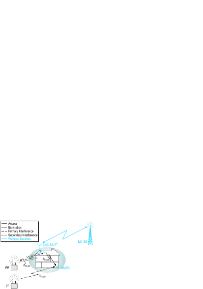
Figure 1: A cognitive small cell scenario demonstrating: (i) the underlay paradigm, (ii) the associated network elements, which constitute Cognitive Small Cell-Base Station/Secondary Transmitter (CSC-BS/ST), Mobile Station/Secondary Receiver (MS/SR), Macro Cell-Base Station (MC-BS) and Primary Transmitter (PT), (iii) the interacting channels: primary interference channel, secondary interference channel and access channel.

II-A Underlay Scenario and Medium Access

The Cognitive Small Cell (CSC), a CR application, characterizes a small cell deployment that fulfills the spectral requirements of the Mobile Stations (MSs) operating indoor, Figure 1. For the disposition of the CSC in the network, the following key elements are essential: a CSC-Base Station (CSC-BS), a Macro Cell-Base Station (MC-BS) and an MS [22]. Considering the fact that the power control is employed at the CSC-BS, the CSC-BS and the MS represent the ST and the SR, respectively. In order to acquire the knowledge concerning the primary interference channel, the ST listens to the transmissions from the PR. In this work, we consider those primary systems where the PR performs transmissions interchangeably over time (time division duplexing TDD and half-duplex frequency division duplexing FDD) or frequency (full-duplex FDD) with the PT. These transmissions can occur over the same band (TDD) or over separate bands (half-duplex and full-duplex FDD). In cellular networks, these duplexing modes are effectively deployed in the Long Term Evolution (LTE) standard [24]. The ST follows these duplexing modes to exploit channel reciprocity principle and determine the interference received at the PR, thus, controls its power for transmitting signals over the access channel such that it satisfies the outage constraint by operating at the IT. Particularly for the half-duplex and the full duplex FDD, it is assumed that the coherence bandwidth is large as compared to the frequency separation between the estimation channel and the band of interest.

We propose to employ a slotted medium access for the US, where the time axis is segmented into frames. As depicted in Figure 2, the frame duration $T$ is chosen in such a way that the frames are aligned to the primary users’ transmissions, i.e., the uplink and the downlink transmissions for the primary and secondary systems occur simultaneously. In this regard, a perfect frame synchronization is assumed between the two systems. In order to incorporate channel estimation, we further propose to employ a periodic channel estimation, according to which the US uses time intervals ($\tau$ and $\tau_{\text{p}}$ in the uplink, and $\tau$ in the downlink) to perform channel estimation followed by data transmission ($T-\tau-\tau_{\text{p}}$ in the uplink and $T-\tau$ in the downlink), see Figure 2. In order to consider variations due to channel fading, we assume that the interacting channels remain constant over at least two frame durations ($2T$). Based on this assumption, every alternating transmission frame observes a different received power, consider Figure 2. Since the channel knowledge is essential to employ the power control so that the primary users are sufficiently protected from the uncertain interference induced due to the imperfect channel knowledge, it is reasonable to carry out estimation for $\tau$ time interval followed by data transmission with controlled power in the remaining time for each frame.

Figure 2: Frame structure of the US illustrating the time allocation for channel estimation and data transmission from the perspective of a ST and a SR. In this regard, corresponding to the uplink and the downlink, the primary interference and secondary interference channel estimation occur at the ST and the SR, respectively. PR (Tx)/PR (Rx) represents the transmission/reception of the primary signal from the PR/PT to the PT/PR.

In accordance with the half duplexing modes, the ST and the SR implement the received power-based estimation to acquire the knowledge of the primary and the secondary interference channel over consecutive frames, as illustrated in Figure 2. For the case where the primary system follows full-duplex FDD, the proposed frame structure can be adapted such that the primary and the secondary interference channel estimation occurs in a single frame. Besides this, the access channel estimation is performed by listening to the pilot symbols transmitted by the SR, classified as the pilot-based channel estimation. At first, we consider the proposed frame structure for a deterministic channel, i.e., the performance is analyzed for a certain channel gain (path-loss channel), without taking into account the effect of channel fading. We then extend the performance analysis for the proposed framework by considering channel fading.

II-B Signal Model

In the uplink, during the estimation phase, the discrete and complex signal received from the PR at the ST is given by

$$y_{\text{ST}}[n]=h_{\text{PR,ST}}\cdot\sqrt{P_{\text{Tx,PR}}}\cdot x_{\text{PR}}[n]+w_{\text{ST}}[n],$$ (1)

where $x_{\text{PR}}[n]$ corresponds to a discrete and complex sample transmitted by the PR with unit power, $P_{\text{Tx,PR}}$ is the transmit power at the PR (known at the ST), $|h_{\text{PR,ST}}|^{2}$ represents the power gain for the primary interference channel and $w_{\text{ST}}[n]$ is circularly symmetric Additive White Gaussian Noise (AWGN) at the ST with $\mathcal{CN}(0,\sigma^{2})$.

In the downlink, during data transmission phase, the interference (received from the ST) plus noise signal at the PR is given by

$$y_{\text{PR}}[n]=h_{\text{PR,ST}}\cdot\sqrt{P_{\text{Tx,ST,cont}}}\cdot x_{\text{ST,cont}}[n]+w_{\text{PR}}[n],$$ (2)

and on the other side, the received signal at the SR follows

$$y_{\text{SR}}[n]= h_{\text{ST,SR}}\cdot\sqrt{P_{\text{Tx,ST,cont}}}\cdot x_{\text{ST,cont}}[n]+$$

$$h_{\text{PT,SR}}\cdot\sqrt{P_{\text{Tx,PT}}}\cdot x_{\text{PT}}[n]+w_{\text{SR}}[n],$$ (3)

where $x_{\text{ST,cont}}[n]$ corresponds to a discrete and complex sample transmitted by the ST with unit power, $P_{\text{Tx,ST,cont}}$ is the controlled transmit power and $x_{\text{PT}}[n]$ is the transmit signal from the PT with transmit power $P_{\text{Tx,PT}}$. Further, $|h_{\text{ST,SR}}|^{2}$ and $|h_{\text{PT,SR}}|^{2}$ represent the power gain for the access channel and the secondary interference channel, respectively. $w_{\text{PR}}[n]$ and $w_{\text{SR}}[n]$ are AWGN at the PR and at the SR, respectively, with $\mathcal{CN}(0,\sigma^{2})$.

II-C Problem Description

According to the existing investigations (also referred as ideal model), an ST of an US is required to control its transmit power in such a way that the interference received ($P_{\text{Rx,PR}}$) at the PR is below IT ($\theta_{\text{I}}$) [3]

$$P_{\text{Rx,PR}}=|h_{\text{PR,ST}}|^{2}P_{\text{Tx,ST,cont}}\leq\theta_{\text{I}}.$$ (4)

After determining the controlled power at the ST using (4), the data rate at the SR over the access channel is defined as

$$\text{C}_{\text{s}}=\log_{2}\left(1+\frac{|h_{\text{ST,SR}}|^{2}P_{\text{Tx,ST,cont}}}{|h_{\text{PT,SR}}|^{2}P_{\text{Tx,PT}}+\sigma^{2}}\right).$$ (5)

From the deployment perspective, the ideal model depicted in (4) and (5) has following issues:

• Without the knowledge of the primary interference channel $h_{\text{PR,ST}}$, it is impossible to employ the power control at the ST, which is based on (4).

• Furthermore, along with $P_{\text{Tx,ST,cont}}$, the knowledge of the access channel $h_{\text{ST,SR}}$ and the secondary interference channel $h_{\text{PT,SR}}$ is required to determine $\text{C}_{\text{s}}$, according to (5).

The ideal model considers the perfect knowledge of the aforementioned channels at the ST, which is not available in practice. In this regard, it is necessary to incorporate channel estimation in the system model. The imperfect channel knowledge, however, translates to the variations in the performance parameters, $P_{\text{Rx,PR}}$ and $\text{C}_{\text{s}}$. Particularly, a variation in $P_{\text{Rx,PR}}$ due to uncertain interference that exceeds $\theta_{\text{I}}$ causes the violation of the outage constraint illustrated in (4). Unless captured, this uncertain interference may seriously degrade the performance of the US. Since the ideal model assumes the perfect knowledge of the involved channels, it is incapable of depicting the degradation in the performance due to the time allocation for the channel estimation and the imperfect knowledge of the channels.

II-D Proposed Approach

In order to facilitate channel estimation for the US, it is essential to take the aforementioned issues into account. To accomplish this, the following strategy is proposed in the paper.

• At first, we consider the estimation of the involved channels. In this regard, we propose to employ a received power-based estimation for the interference channels and a pilot-based estimation for the access channel.

• To capture the effect of the imperfect channel knowledge, we characterize the variations in the estimated parameters (namely, received power for the interference channels and power gain for the access channels) in terms of their cdfs.

• The aforementioned variations are translated to the performance parameters, which include the uncertain interference and the secondary throughput. We further characterize these variation in the performance parameters in terms of their cdfs. More specifically, using the characterization of the uncertain interference, we propose a novel power control mechanism that regulates the uncertain interference at the PR.

• Finally, using the derived expressions, we analyze a relationship between the estimation time and the expected secondary throughput for the US. We extend the proposed framework (also referred as estimation model) to analyze the impact of channel fading on the performance of the system.

Since the channel estimation in the context of CR systems involves different systems, suitable channel estimation techniques should be selected such that the following requirements: (i) low complexity and (ii) versatility towards unknown primary user signals, essential from the deployment perspective, are respected. Similar problem for the interweave CR systems has been deeply investigated in [22], where the authors propose to employ a received power-based estimation for the channels between the primary and the secondary systems and a pilot-based estimation for the access channel. Following a similar strategy, we propose to employ received power-based and pilot-based estimation techniques in the underlay CR systems. It is also worth stating that, since the signal model in [22] (orthogonal frequency division multiplexing transmission) differs from the one (constant power transmission) studied in this paper, we derive new mathematical expressions for the performance parameters. In the following paragraphs, we consider the estimation of the power gains of the primary interference channel $|\hat{h}_{\text{PR,ST}}|^{2}$, the access channel $|\hat{h}_{\text{ST,SR}}|^{2}$ and the secondary interference channel $|\hat{h}_{\text{PR,SR}}|^{2}$.

II-D1 Estimation of primary interference channel

Considering

$$P_{\text{Rx,ST}}=|h_{\text{PR,ST}}|^{2}P_{\text{Tx,PR}}+\sigma^{2},$$ (6)

and the knowledge of PR’s transmit power $P_{\text{Tx,PR}}$, the ST employs received power-based estimation to obtain the knowledge of $|h_{\text{PR,ST}}|^{2}$. To accomplish this, in reference to (1), the ST listens to the transmissions from the PR and acquires the knowledge of $|h_{\text{PR,ST}}|^{2}$ indirectly by estimating the power received in the uplink as $\hat{P}_{\text{Rx,ST}}={\frac{1}{{\tau f_{\text{s}}}}\sum_{n}^{\tau f_{\text{s}}}}{|y_{\text{ST}}[n]|^{2}}$, where $f_{\text{s}}$ being the sampling frequency and $\tau$ represents the estimation time interval. $f_{\text{s}}$ and $\tau$ are such that the number of samples $\tau f_{\text{s}}$ is an integer. The estimated received power $\hat{P}_{\text{Rx,ST}}$ is utilized to determine the controlled power $P_{\text{Tx,ST,cont}}$ at which the data transmission over the downlink is carried out, consider Figure 2. In accordance to the received power-based estimation for the primary interference channel in (6), it is noticed that the knowledge of $P_{\text{Tx,PR}}$ at the ST is essential for the characterization of the controlled power (considered later in Lemma 4). This knowledge can be retrieved from the specification of different wireless standards such as GSM, EDGE and LTE, etc. [26]. It is well-known that certain standards follow adaptive modulation and coding, which can consequently change $P_{\text{Tx,PR}}$. Under this situation, the ST can employ more complex techniques such as pilot assisted techniques in order to determine $P_{\text{Tx,PR}}$ for the given frame.

For a certain value of $|h_{\text{PR,ST}}|^{2}$, the received power at the ST estimated using $\tau f_{\text{s}}$ samples follows a non-central chi-squared distribution $F_{\hat{P}_{\text{Rx,ST}}}\sim\operatorname*{{\mathcal{X}^{\prime}}^{2}}2(\lambda_{\text{p,1}},\tau f_{\text{s}})$ with non-centrality parameter $\lambda_{\text{p,1}}=\tau f_{\text{s}}|h_{\text{PR,ST}}|^{2}P_{\text{Tx,PR}}/\sigma^{2}=\tau f_{\text{s}}\gamma$ [27], where $\gamma$ is defined as the ratio of the received signal power (from the PR) to noise at the ST and $\tau f_{\text{s}}$ corresponds to the degrees of freedom. For analytical tractability, we consider the following approximation.

Approximation 1

For all degrees of freedom, the $\operatorname*{{\mathcal{X}^{\prime}}^{2}}2$ distribution can be approximated by a Gamma distribution [28]. The parameters of the Gamma distribution are obtained by matching the first two central moments to those of $\operatorname*{{\mathcal{X}^{\prime}}^{2}}2$.

Lemma 1

The cdf of $\hat{P}_{\text{Rx,ST}}$ is characterized as

$$F_{\hat{P}_{\text{Rx,ST}}}(x)\approx 1-\Gamma \left(a_{\text{p,1}},\frac{x}{b_{\text{p,1}}}\right),$$ (7)

$$\text{where }a_{\text{p,1}}=\frac{\tau f_{\text{s}}(1+\gamma)^{2}}{2+4\gamma} \text{ and }b_{\text{p,1}}=\frac{\sigma^{2}(2+4\gamma)}{\tau f_{\text{s}}(1+\gamma)},$$ (8)

and $\Gamma(\cdot,\cdot)$ represents the regularized upper-incomplete Gamma function [28].

Proof:

Applying Approximation 1 to $\operatorname*{{\mathcal{X}^{\prime}}^{2}}2(\lambda_{\text{p,1}},\tau f_{\text{s}})$ yields (7). ∎

II-D2 Estimation of access channel

In the uplink, the discrete and complex pilot signal transmitted by the SR undergoes matched filtering and demodulation at the ST, consider Figure 2, hence, we employ a pilot-based estimation at the ST to acquire the knowledge of the access channel. According to [29], the maximum-likelihood estimate with $\tau_{\text{p}}{f_{\text{s}}}$ pilot symbols is given by

$$\hat{h}_{\text{s}}=h_{\text{ST,SR}}+\frac{\sum^{\tau_{\text{p}}{f_{\text{s}}}}_{n=1}w_{\text{ST}}[n]}{\tau_{\text{p}}{f_{\text{s}}}},$$ (9)

where $\frac{\sum^{\tau_{\text{p}}{f_{\text{s}}}}_{n}w_{\text{ST}}[n]}{\tau_{\text{p}}{f_{\text{s}}}}$ represents the estimation error. With no loss of generality, the pilot symbols are considered to be $+1$. As a result, the estimate $\hat{h}_{\text{s}}$ is unbiased, efficient, i.e., achieves the Cramér-Rao bound with equality, with asymptotic variance ${\mathbb{E}}\left[|h_{\text{ST,SR}}-\hat{h}_{\text{s}}|^{2}\right]=\frac{\sigma^{2}}{\tau_{\text{p}}{f_{\text{s}}}}$ [29]. Hence, $\hat{h}_{\text{s}}$ conditioned on $h_{\text{ST,SR}}$ follows a circularly symmetric Gaussian distribution, given by

$$\hat{h}_{\text{s}}|h_{\text{ST,SR}}\sim\mathcal{C}\mathcal{N}\left(h_{\text{ST,SR}},\frac{\sigma^{2}}{\tau_{\text{p}}{f_{\text{s}}}}\right).$$ (10)

Consequently, for a certain value of $|h_{\text{ST,SR}}|^{2}$, the estimated power gain $|\hat{h}_{\text{s}}|^{2}$ follows a non-central chi-squared $\operatorname*{{\mathcal{X}^{\prime}}^{2}}2(\lambda_{\text{s}},2)$ distribution with 2 degrees of freedom and non-centrality parameter $\lambda_{\text{s}}=\frac{\tau_{\text{p}}{f_{\text{s}}}|h_{\text{ST,SR}}|^{2}}{\sigma^{2}}$.

Lemma 2

The cdf of $|\hat{h}_{\text{ST,SR}}|^{2}$ is characterized as

$$F_{|\hat{h}_{\text{ST,SR}}|^{2}}(x)\approx 1-\Gamma \left(a_{\text{s}},\frac{x}{b_{\text{s}}}\right),$$ (11)

$$\text{where }a_{\text{s}}=\frac{(2+\lambda_{\text{s}})^{2}}{4+4\lambda_{\text{s}}} \text{ and }b_{\text{s}}=\frac{\sigma^{2}(4+4\lambda_{\text{s}})}{(2+\lambda_{\text{s}})}.$$ (12)

Proof:

Applying Approximation 1 to $\operatorname*{{\mathcal{X}^{\prime}}^{2}}2(\lambda_{\text{s}},2)$ yields (11). ∎

II-D3 Estimation of secondary interference channel

In the downlink, the SR estimates the interference (power) received from the PT, consider (3). The power estimated over the signal $h_{\text{PT,SR}}\cdot\sqrt{P_{\text{Tx,PT}}}\cdot x_{\text{PT}}[n]+w_{\text{SR}}[n]$ corresponds to the interference plus noise power ($P_{\text{Rx,SR}}=|h_{\text{PT,SR}}|^{2}P_{\text{Tx,PR}}+\sigma^{2}$, where $P_{\text{Rx,SR}}$ represents the true value, consider (5)). The estimated received power at the SR is determined as $\hat{P}_{\text{Rx,SR}}={\frac{1}{{\tau f_{\text{s}}}}\sum_{n}^{\tau f_{\text{s}}}}{|h_{\text{PT,SR}}\cdot\sqrt{P_{\text{Tx,PT}}}\cdot x_{\text{PT}}[n]+w_{\text{SR}}[n]|^{2}}$. To characterize the secondary throughput, $\hat{P}_{\text{Rx,SR}}$ is made available to the ST over a low rate feedback channel. Similar to $\hat{P}_{\text{Rx,ST}}$, for a certain value of $|h_{\text{PT,SR}}|^{2}$, $\hat{P}_{\text{Rx,SR}}$ follows a non-central chi-squared distribution $\operatorname*{{\mathcal{X}^{\prime}}^{2}}2(\lambda_{\text{p,2}},\tau f_{\text{s}})$, with non-centrality parameter $\lambda_{\text{p,2}}=\tau f_{\text{s}}|h_{\text{PT,SR}}|^{2}P_{\text{Tx,PT}}/\sigma^{2}$.

Lemma 3

The cdf of $\hat{P}_{\text{Rx,SR}}$ is characterized as

$$F_{\hat{P}_{\text{Rx,SR}}}(x)\approx 1-\Gamma \left(a_{\text{p,2}},\frac{x}{b_{\text{p,2}}}\right),$$ (13)

$$\text{where }a_{\text{p,2}}=\frac{(\tau f_{\text{s}}+\lambda_{\text{p,2}})^{2}}{2\tau f_{\text{s}}+4\lambda_{\text{p,2}}} \text{ and }b_{\text{p,2}}=\frac{\sigma^{2}(2\tau f_{\text{s}}+4\lambda_{\text{p,2}})}{(\tau f_{\text{s}}+\lambda_{\text{p,2}})}.$$ (14)

Proof:

Applying Approximation 1 to $\operatorname*{{\mathcal{X}^{\prime}}^{2}}2(\lambda_{\text{p,2}},\tau f_{\text{s}})$ yields (13). ∎

It is important to note that, in this paper, we are dealing with a single PT and a single PR. However, in practice, it is possible that the ST and the SR accumulate significant interference (defined as aggregate interference) from other PRs and PTs (co-channel interference due to frequency reuse) in the network[30, 31] over the primary interference channel and the secondary interference channel, respectively. For the secondary interference channel, the only difference is that the SR now estimates the aggregate interference. Due to this, the expression of $\hat{P}_{\text{Rx,SR}}$ in the secondary throughput remains unchanged. On the other side, by estimating the aggregate interference on the primary interference channel, the ST overestimates $\hat{P}_{\text{Rx,ST}}$ and exercises a greater power control. Even for such a case, the outage constraint on the primary interference channel to the desired PR is satisfied, however, reduces the secondary throughput.

III Theoretical Analysis

III-A Deterministic Channel

In this section, we investigate the performance of the US for a specific frame. In this sense, the involved channels $h_{\text{PR,ST}}$, $h_{\text{PT,SR}}$ and $h_{\text{ST,SR}}$ are deterministic (not random). First, we employ an outage probability constraint $\rho_{\text{out}}$ on the interference to capture the variations in the $P_{\text{Rx,PR}}$ incurred due to channel estimation, defined as

$$\mathbb{P}\left(P_{\text{Rx,PR}}=|\hat{h}_{\text{PR,ST}}|^{2}P_{\text{Tx,ST,cont}}\geq\theta_{\text{I}}\right)\leq\rho_{\text{out}}.$$ (15)

Substituting $$|\hat{h}_{\text{PR,ST}}|^{2}$$ from (6) yields

$$\mathbb{P}\left(\left(\frac{\hat{P}_{\text{Rx,ST}}-\sigma^{2}}{P_{\text{Tx,PR}}}\right)P_{\text{Tx,ST,cont}}\geq\theta_{\text{I}}\right)\leq\rho_{\text{out}}.$$ (16)

Besides the outage constraint, $P_{\text{Tx,ST,cont}}$ is limited by a predefined transmit power $P_{\text{Tx,ST,full}}$. To capture this aspect, the transmit power constraint at the ST is defined as

$$P_{\text{Tx,ST,cont}}\leq P_{\text{Tx,ST,full}}.$$ (17)

We consider that the same power is allocated to all the symbols transmitted within a frame by the ST. In this regard, the transmit power constraint on symbol basis and frame basis is equivalent. As a consequence, the constraint depicted in (17) is applicable to both the cases. Based on the constraints in (16) and (17), we subsequently determine the expression of the controlled power for the proposed framework.

Lemma 4

Subject to the outage constraint on the uncertain interference and the transmit power constraint at the ST, the controlled power at the ST is given by

$$P_{\text{Tx,ST,cont}} =\begin{cases}\frac{\theta_{\text{I}}P_{\text{Tx,PR}}}{\left(b_{\text{p,1}}\Gamma^{-1}(\rho_{\text{out}},a_{\text{p,1}})-\sigma^{2}\right)},&\mbox{for }P_{\text{Tx,ST,cont}}<P_{\text{Tx,ST,full}}\\ P_{\text{Tx,ST,full}},&\mbox{for }P_{\text{Tx,ST,cont}}\geq P_{\text{Tx,ST,full}}\end{cases},$$ (18)

where $a_{\text{p,1}}$ and $b_{\text{p,1}}$ are defined in (8) and $\Gamma^{-1}(\cdot,\cdot)$ is the inverse function of regularized upper-incomplete Gamma function [28].

Proof:

Substituting the cdf $F_{\hat{P}_{\text{Rx,ST}}}(x)$, defined in (7), in (16) and combining with (17) yields (18). ∎

Clearly, the performance of the US improves over the access channel (in terms of the secondary throughput) with $P_{\text{Tx,ST,cont}}$, but $P_{\text{Tx,ST,cont}}$ increases for the values of $|h_{\text{PR,ST}}|^{2}$, which correspond to the lower values of $\gamma$. However, in practice, the wireless systems are limited by the transmit power $P_{\text{Tx,ST,full}}$, which bounds the performance of the US. In order to understand the effect of the power limitation on the US, we characterize a performance bound in terms of the estimation time.

Corollary 1

Subject to the outage constraint on the uncertain interference and the transmit power constraint at the ST, the performance bound ($\gamma^{*}$) of the US is defined as

$$\Gamma\left(\frac{\tau f_{\text{s}}(1+\gamma^{*})^{2}}{2+4\gamma^{*}},\frac{\tau f_{\text{s}}(1+\gamma^{*})}{\sigma^{2}(2+4\gamma^{*})}\left(\frac{\theta_{\text{I}}P_{\text{Tx,PR}}}{P_{\text{Tx,ST,full}}}+\sigma^{2}\right)\right)=\rho_{\text{out}}.$$ (19)

Proof:

Substituting $P_{\text{Tx,ST,cont}}$ with $P_{\text{Tx,ST,full}}$ in (16) and reformulating gives

$$\mathbb{P}\left(\hat{P}_{\text{Rx,ST}}\geq\frac{\theta_{\text{I}}P_{\text{Tx,PR}}}{P_{\text{Tx,ST,full}}}+\sigma^{2}\right) \leq\rho_{\text{out}}.$$ (20)

Using (7) in Lemma 1 gives

$$\Gamma\left(\frac{\tau f_{\text{s}}(1+\gamma)^{2}}{2+4\gamma},\frac{\tau f_{\text{s}}(1+\gamma)}{\sigma^{2}(2+4\gamma)}\left(\frac{\theta_{\text{I}}P_{\text{Tx,PR}}}{P_{\text{Tx,ST,full}}}+\sigma^{2}\right)\right) \leq\rho_{\text{out}}.$$ (21)

Substituting $\gamma$ with $\gamma^{*}$ and replacing the expression in (21) with equality yields (19). ∎

Figure 3: An illustration of the performance bound ($\gamma^{*}$) for the US depicted in terms of estimation time ($\tau$), where $\gamma$ represents the ratio of the received power (from the PR) to noise at the ST. It further classifies the operation of the US as the interference-limited and the power-limited regimes.

Remark 1

Figure 3 analyzes the variations of $\gamma^{*}$ with $\tau$. Using the expression $\gamma^{*}$ obtained in Corollary 1, we classify the operation of the US into the following regimes: (i) interference-limited regime and (ii) power-limited regime. Inside the interference-limited regime $\gamma>\gamma^{*}$, due to good quality of the channel ST-PR (unfavorable to the US), the system is limited due to the exceeding level of the uncertain interference, which can be regulated effectively by employing power control at the US to satisfy the given outage constraint ($\rho_{\text{out}}$). At $\gamma=\gamma^{*}$, the ST operates at the maximum allowable power $P_{\text{Tx,ST,cont}}=P_{\text{Tx,ST,full}}$ while respecting the tolerance limits defined for the uncertain interference. From a different perspective, the situation $\gamma=\gamma^{*}$ also represents those USs that are unable to carry out power control. With regard to the outage constraint and the lack of the power control, for a given choice of $\gamma^{*}$, such systems can operate only at a specific value of $\tau$.

On the other side, the region $\gamma<\gamma^{*}$, which depicts a weak link quality between the ST and the PR, is beneficial to the secondary user. However, due to the transmit power constraint, the USs can operate at or below $P_{\text{Tx,ST,full}}$. As a result, these favorable conditions do not translate to any performance gain. Therefore, this regime is characterized as a power-limited regime. Besides, it is interesting to observe that for small values of the estimation time, $\gamma^{*}\rightarrow-\infty$, which signifies that low $\tau$ increases the uncertainty in the interference. In order to regulate the level of this uncertainty, US has to be proactive in terms of the power control to be able to satisfy the outage constraint. It is also observed that as $\tau\rightarrow\infty$, $\gamma^{*}$ converges asymptotically to a certain value. This signifies the fact that, beyond a certain value, the time resources allocated for the channel estimation do not account to any significant improvement in the terms of the uncertain interference or indirectly in terms of the controlled power. As a result, the performance of the US in the form of controlled power gets saturated, thus, limiting the performance of the US in terms of the secondary throughput.

Next, we capture the variations in the secondary throughput in terms of its expected value. To accomplish this, the cdf of the estimated data rate, given by

$$\hat{\text{{C}}}_{\text{s}}=\log_{2}\left(1+\frac{|\hat{h}_{\text{ST,SR}}|^{2}P_{\text{Tx,ST,cont}}}{\hat{P}_{\text{Rx,SR}}}\right)$$ (22)

is evaluated over the access channel at the ST. It is worth noticing the fact that unlike $\text{C}_{\text{s}}$ defined in (5), $\hat{\text{{C}}}_{\text{s}}$ entails the random behavior due to the estimation of $|\hat{h}_{\text{ST,SR}}|^{2}$ and $\hat{P}_{\text{Rx,SR}}$.

Lemma 5

The cdf of data rate $\hat{\text{{C}}}_{\text{s}}$ is given by

$$F_{\hat{\text{{C}}}_{\text{s}}}(x) =\int\limits_{0}^{x}f_{\hat{\text{{C}}}_{\text{s}}}(t)dt,$$ (23)

where the pdf is given by

$$f_{\hat{\text{{C}}}_{\text{s}}}(x)= 2^{x}\ln 2\frac{(2^{x}-1)^{a_{\text{s}}-1}\Gamma(a_{\text{s}}+a_{\text{p,2}})}{\Gamma(a_{\text{s}})\Gamma(a_{\text{p,2}})(b_{\text{s}}P_{\text{Tx,ST,cont}})^{a_{\text{s}}}b_{\text{p,2}}^{a_{\text{p,2}}}}\times$$

$$\left(\frac{1}{b_{\text{p,2}}}+\frac{2^{x}-1}{b_{\text{s}}P_{\text{Tx,ST,cont}}}\right).$$ (24)

Proof:

See Appendix V. ∎

(a)

(b)

Figure 4: CDF of $\hat{\text{{C}}}_{\text{s}}$ for different received interference to noise ratio $\frac{|h_{\text{PT,SR}}|^{2}P_{\text{Tx,PT}}}{\sigma^{2}}$ over the secondary interference channel and estimation time $\tau$. (a) $\frac{|h_{\text{PT,SR}}|^{2}P_{\text{Tx,PT}}}{\sigma^{2}}\in\{-10,0,10\}$\text{\,}\mathrm{d}\mathrm{B}$$ and $\tau=$1\text{\,}\mathrm{m}\mathrm{s}$$, (b) $\tau=\{0.1,1,10\}$\text{\,}\mathrm{m}\mathrm{s}$$ and $\frac{|h_{\text{PT,SR}}|^{2}P_{\text{Tx,PR}}}{\sigma^{2}}=$0\text{\,}\mathrm{d}\mathrm{B}$$, for the following values of the system parameters, $\gamma=$10\text{\,}\mathrm{d}\mathrm{B}$$, $P_{\text{Tx,ST,cont}}=$0\text{\,}\mathrm{d}\mathrm{B}\mathrm{m}$$. The solid line represents the values computed using the analytical expressions while the markers represent the values obtained from the simulations.

In consideration to the Approximation 1, which is applied to obtain the cdfs’ of $\hat{P}_{\text{Rx,ST}}$, $|\hat{h}_{\text{ST,SR}}|^{2}$ and $\hat{P}_{\text{Rx,SR}}$ in Lemma 5, the theoretical expression of the cdf depicted in (23) is validated by means of simulations in Figure 4 with different choices of the system parameters, which include $\gamma=$10\text{\,}\mathrm{d}\mathrm{B}$$, $P_{\text{Tx,ST,cont}}=$0\text{\,}\mathrm{d}\mathrm{B}\mathrm{m}$$, $\frac{|h_{\text{PT,SR}}|^{2}P_{\text{Tx,PT}}}{\sigma^{2}}\in\{-10,0,10\}$\text{\,}\mathrm{d}\mathrm{B}$$ and $\tau=\{0.1,1,10\}$\text{\,}\mathrm{m}\mathrm{s}$$.

Besides the outage constraint on the uncertain interference, the expected secondary throughput (averaged over $2T$ frame durations, which include the uplink and the downlink transmissions, consider Figure 2) over the access channel at the SR is defined as

$$R_{\text{s}}(\tau) =\frac{T-\tau-\frac{\tau_{\text{p}}}{2}}{T}{\mathbb{E}}_{\hat{\text{{C}}}_{\text{s}}}\left[\hat{\text{{C}}}_{\text{s}}\right],$$ (25)

where ${\mathbb{E}}_{\hat{\text{{C}}}_{\text{s}}}\left[\cdot\right]$ corresponds to an expectation over $\hat{\text{{C}}}_{\text{s}}$, whose pdf is characterized in Lemma 5.

Remark 2

At this point, it is well-known that the performance degradation due to channel estimation in the form of the secondary throughput is inherent to the US. Specifically, the time allocation and the uncertain interference are responsible of this degradation. The controlled power, determined in Lemma 4, characterized as a function of the estimation time allows us to regulate the uncertain interference. As discussed previously in Remark 1, the low estimation time enables a severe control in power, thereby decreasing the secondary throughput. On the other hand, less time resources allocated for the channel estimation increases the secondary throughput. This phenomenon can be captured by observing the variation of the secondary throughput along the estimation time such that the constraints depicted in (16) and (17) are fulfilled. Below, Problem 1 captures this relationship between the estimation time and the secondary throughput defined as an estimation-throughput tradeoff. More importantly, we utilize this tradeoff to determine a suitable estimation time at which the maximum throughput at the SR is achieved.

Problem 1

The achievable expected secondary throughput subject to the outage constraint on the uncertain interference and the transmit power constraint at the ST is defined as

$$R_{\text{s}}(\tilde{\tau})=\operatorname*{max}_{\tau} \text{ }{R_{\text{s}}(\tau)},$$ (26)

s.t. $$\text{ }(\ref{eq:opc}),\text{ }(\ref{eq:pc}),$$

where $R_{\text{s}}(\tilde{\tau})$ corresponds to optimum throughput at $\tilde{\tau}$.

Proof:

The constrained optimization problem is solved by substituting $P_{\text{Tx,ST,cont}}$ from Lemma 3, determined by applying the outage and the transmit power constraints defined in (16) and (17), in (25). The pdf of $\hat{\text{{C}}}_{\text{s}}$, determined in (24), is used to evaluate the expectation. Following this, we obtain an expression of the expected secondary throughput as a function of $\tau$

$$R_{\text{s}}(\tau)=\frac{T-\tau-\frac{\tau_{\text{p}}}{2}}{T}\int\limits_{0}^{\infty}xf_{\hat{\text{{C}}}_{\text{s}}}(x)dx.$$ (27)

Solving numerically the expression in (27) yields $\tilde{\tau}$ and $R_{\text{s}}(\tilde{\tau})$. ∎

Corollary 2

Problem 1 considers the optimization of the expected secondary throughput for the proposed framework that employ power control and considers the effect of the imperfect channel knowledge. In accordance to Corollary 1, these USs correspond to the USs that operate in the interference-limited regime $\gamma^{*}\geq\gamma$. Besides, it is interesting to compare its performance with those USs that employ channel estimation (as proposed in the paper) and satisfy the outage constraint on the uncertain interference, however, employ no power control, i.e., operate at $P_{\text{Tx,ST,full}}$. With regard to Corollary 1, these systems correspond to the ones operating on the curve $\gamma^{*}=\gamma$. For the latter approach, the secondary throughput is obtained by substituting $P_{\text{Tx,ST,cont}}$ with $P_{\text{Tx,ST,full}}$ in (25), where $\tau$ in (25) is determined using Corollary 1. Such a comparison allows us to quantify the performance gain procured by the US when power control is employed at the ST.

III-B Random Channel

Here, our objective is to investigate the performance of the proposed approach, where the interacting channels encounter quasi-static block fading. Specifically, the performance of the US is analyzed over multiple frames, where every alternating transmission according to the frame structure presented in Figure 2 observes a different channel. In this regard, we characterize the channel gains $h_{\text{PR,ST}}$, $h_{\text{PT,SR}}$ and $h_{\text{ST,SR}}$ according to Nakagami-$m$ fading model. As a consequence, the power gains $|h_{\text{PR,ST}}|^{2}$, $|h_{\text{PT,SR}}|^{2}$ and $|h_{\text{ST,SR}}|^{2}$ follow a Gamma distribution [32], whose corresponding cdfs are defined as

$$F_{|h_{\text{PR,ST}}|^{2}}(x)=1-\Gamma\left(m_{\text{PR,ST}},\frac{m_{\text{PR,ST}}x}{|\bar{h}_{\text{PR,ST}}|^{2}}\right),$$ (28)

$$F_{|h_{\text{PT,SR}}|^{2}}(x)=1-\Gamma\left(m_{\text{PT,SR}},\frac{m_{\text{PT,SR}}x}{|\bar{h}_{\text{PT,SR}}|^{2}}\right),$$ (29)

$$F_{|h_{\text{ST,SR}}|^{2}}(x)=1-\Gamma\left(m_{\text{ST,SR}},\frac{m_{\text{ST,SR}}x}{|\bar{h}_{\text{ST,SR}}|^{2}}\right),$$ (30)

where $m_{\text{PR,ST}}$, $m_{\text{PT,SR}}$ and $m_{\text{ST,SR}}$ represent the $m$ parameter, whereas $|\bar{h}_{\text{PR,ST}}|^{2}$, $|\bar{h}_{\text{PT,SR}}|^{2}$ and $|\bar{h}_{\text{ST,SR}}|^{2}$ are the expected values for channels $|h_{\text{PR,ST}}|^{2}$, $|h_{\text{PT,SR}}|^{2}$ and $|h_{\text{ST,SR}}|^{2}$, respectively. The performance analysis subject to channel fading has been considered by Ghasemi et al. [33, 4], where the authors in [33, 4] evaluated the expected data rate while constraining the interference at the PR. The influence of channel fading (however, without channel estimation signifying the perfect channel knowledge) has been quantified in terms of the outage constraint on the uncertain interference, is given by

$$\operatorname*{max}_{P_{\text{Tx,ST,cont}}} \text{ }{\mathbb{E}}_{|h_{\text{PT,SR}}|^{2},|h_{\text{ST,SR}}|^{2}}\left[\text{C}_{\text{s}}\right],$$ (31)

s.t. $$\text{ }\mathbb{P}(P_{\text{Rx,PR}}=|h_{\text{PR,ST}}|^{2}P_{\text{Tx,ST,cont}}\geq\theta_{\text{I}})\leq\rho_{\text{out}},$$ (32)

where ${\mathbb{E}}_{|h_{\text{PT,SR}}|^{2},|h_{\text{ST,SR}}|^{2}}\left[\cdot\right]$ corresponds to an expectation with respect to $|h_{\text{PT,SR}}|^{2},|h_{\text{ST,SR}}|^{2}$, which are entailed in $\text{C}_{\text{s}}$, refer to (5).

Despite the knowledge of the fading model, similar to the ideal model depicted for the deterministic channel (Section II-C), the characterization in (31) and (32) assumes the perfect knowledge of the realizations of the power gains $(|h_{\text{PR,ST}}|^{2},|h_{\text{PT,SR}}|^{2},|h_{\text{ST,SR}}|^{2})$ for the corresponding channels. In view of this, we extend our proposed framework to investigate the effect of the random channel (channel fading) on the performance of the US.

In this regard, we first determine the expression of the outage constraint on the uncertain interference

$$\smash[b]{\overbrace{{\mathbb{E}}_{|h_{\text{PR,ST}}|^{2}}\left[\smash[b]{\underbrace{\mathbb{P}\left(\left(\frac{\hat{P}_{\text{Rx,ST}}-\sigma^{2}}{P_{\text{Tx,PR}}}\right)P_{\text{Tx,ST,cont}}\geq\theta_{\text{I}}\right)}_{\text{Channel Estimation}}}\right]}^{\text{Channel Fading}}}\leq\rho_{\text{out}},$$ (33)

where $\hat{P}_{\text{Rx,ST}}$ depends on the underlying value of $|h_{\text{PR,ST}}|^{2}$, which is a random variable. In contrast to the constraint in (32), (33) captures the variations due to the channel estimation $(\mathbb{P}(\cdot)$ determined in terms of $\hat{P}_{\text{Rx,ST}}$) and the channel fading (${\mathbb{E}}_{|h_{\text{PR,ST}}|^{2}}\left[\cdot\right]$). Based on (33) and transmit power constraint defined in (17), we further obtain the expression of the controlled power $(P_{\text{Tx,ST,cont}})$ for the case with random channel.

Lemma 6

Subject to the outage constraint on the uncertain interference and the transmit power constraint at the ST, the controlled power at the ST under Nakagami-$m$ fading is given by (see top of next page)

$$P_{\text{Tx,ST,cont}} =\begin{cases}\int\limits_{0}^{\infty}\Gamma\left(\frac{\tau f_{\text{s}}(1+xP_{\text{Tx,PR}}/\sigma^{2})^{2}}{2+4xP_{\text{Tx,PR}}/\sigma^{2}},\frac{\tau f_{\text{s}}(1+xP_{\text{Tx,PR}}/\sigma^{2})}{\sigma^{2}(2+4xP_{\text{Tx,PR}}/\sigma^{2})}\left(\frac{\theta_{\text{I}}P_{\text{Tx,PR}}}{P_{\text{Tx,ST,cont}}}+\sigma^{2}\right)\right)dF_{|h_{\text{PR,ST}}|^{2}}(x)=\rho_{\text{out}},&\mbox{for }P_{\text{Tx,ST,cont}}<P_{\text{Tx,ST,full}}\\ P_{\text{Tx,ST,full}},&\mbox{for }P_{\text{Tx,ST,cont}}\geq P_{\text{Tx,ST,full}}\end{cases}.$$ (34)

, where $F_{|h_{\text{PR,ST}}|^{2}}(\cdot)$ is defined in (28).

Proof:

Since it is complicated to obtain a closed form expression of the integral in (34), we evaluate the controlled power numerically. ∎

Similar to analysis performed in Corollary 1 for the deterministic channel, below, we determine the performance bound $(\gamma^{*})$ in terms of $\tau$ for the random channel. To this end, we substitute $P_{\text{Tx,ST,cont}}$ with $P_{\text{Tx,ST,full}}$ in the expression (34)

$$\int\limits_{0}^{\infty}\Gamma\Bigg{(}\frac{\tau f_{\text{s}}(1+xP_{\text{Tx,PR}}/\sigma^{2})^{2}}{2+4xP_{\text{Tx,PR}}/\sigma^{2}},\frac{\tau f_{\text{s}}(1+xP_{\text{Tx,PR}}/\sigma^{2})}{\sigma^{2}(2+4xP_{\text{Tx,PR}}/\sigma^{2})}\times$$

$$\left(\frac{\theta_{\text{I}}P_{\text{Tx,PR}}}{P_{\text{Tx,ST,full}}}+\sigma^{2}\right)\Bigg{)}dF_{|h_{\text{PR,ST}}|^{2}}(x) \leq\rho_{\text{out}}.$$ (35)

In order to obtain $\gamma^{*}$, we evaluate the integral on the left side to obtain function of $|h_{\text{PR,ST}}|^{2}$ and $\tau$. Since no closed form expression of this function is obtained, we represent this function as

$$g(|h_{\text{PR,ST}}|^{2},\tau f_{\text{s}})\leq\rho_{\text{out}}.$$

Substituting $|h_{\text{PR,ST}}|^{2}=\frac{\gamma^{*}\sigma^{2}}{P_{\text{Tx,PR}}}$ and replacing with equality, we determine $\gamma^{*}$ for the random channel as

$$g\left(\frac{\gamma^{*}\sigma^{2}}{P_{\text{Tx,PR}}},\tau f_{\text{s}}\right) =\rho_{\text{out}}.$$

Figure 5: An extension of the interference-limited and the power-limited regimes for the US to the random channels, where the channels are subject to Nakagami-$m$ fading. The performance bound ($\gamma^{*}$) is depicted in terms of estimation time ($\tau$). The different curves demonstrates the severity $(m\in\{0,5,1,2,5,\infty\})$ in fading observed by the channels.

Remark 3

Figure 5 analyzes the variation of $\gamma^{*}$ with $\tau$ for different $m\in\{0.5,1,2,5,\infty\}$, where $m=\infty$ represents a deterministic channel. It is observed that $\gamma^{*}$ attains a lower value as the channel fading becomes severe, thereby enabling the US to operate at low $\gamma$ by extending the interference-limited regime. Following the analysis from Remark 1, this also reflects that the power control becomes proactive as the severity in the fading increases. In addition, it is noticed that the deterministic channel is more sensitive to the estimation time as compared to the random channels.

After determining the controlled power in Lemma 6 that regulates the uncertain interference, we determine the expression of the secondary throughput.

$$R_{\text{s}}(\tau) ={\mathbb{E}}_{\hat{\text{{C}}}_{\text{s}},|h_{\text{PT,SR}}|^{2},|h_{\text{ST,SR}}|^{2}}\left[\frac{T-\tau-\frac{\tau_{\text{p}}}{2}}{T}\hat{\text{{C}}}_{\text{s}}\right],$$ (36)

where ${\mathbb{E}}_{\hat{\text{{C}}}_{\text{s}},|h_{\text{PT,SR}}|^{2},|h_{\text{ST,SR}}|^{2}}\left[\cdot\right]$ corresponds to an expectation over $\hat{\text{{C}}}_{\text{s}}$, $|h_{\text{PT,SR}}|^{2}$ and $|h_{\text{ST,SR}}|^{2}$, whose cdfs are characterized in Lemma 5, (29) and (30), respectively. It is worth noticing that $\hat{\text{{C}}}_{\text{s}}$ captures the variations due to channel estimation $|\hat{h}_{\text{ST,SR}}|^{2}$ and $\hat{P}_{\text{Rx,ST}}$, (22), however, due to channel fading, the underlying values of the channels $|h_{\text{PT,SR}}|^{2}$ and $|h_{\text{ST,SR}}|^{2}$ are random. In this context, we perform an expectation with respect to $|h_{\text{PT,SR}}|^{2}$ and $|h_{\text{ST,SR}}|^{2}$, as depicted in (36). Similar to the deterministic channel, we characterize the estimation-throughput tradeoff for the random channel.

Problem 2

The achievable expected secondary throughput subject to the outage constraint on the uncertain interference and the transmit power constraint at the ST under Nakagami-$m$ fading is defined as

$$R_{\text{s}}(\tilde{\tau})=\operatorname*{max}_{\tau} \text{ }{R_{\text{s}}(\tau)},$$ (37)

s.t. $$\text{ }(\ref{eq:opc_fad}),\text{ }(\ref{eq:pc}),$$

where $R_{\text{s}}(\tilde{\tau})$ corresponds to optimum throughput at $\tilde{\tau}$.

Corollary 3

Here, we extend the approach depicted in Corollary 2 to study the performance of those USs that employ channel estimation, operates without power control, satisfy the outage constraint and are subjected to Nakagami-$m$ fading. The expected secondary throughput for this particular approach is obtained by replacing $P_{\text{Tx,ST,cont}}$ in the expression in (36) with $P_{\text{Tx,ST,full}}$, where $\tau$ is determined using (35).

IV Numerical Analysis

In this section, we evaluate the performance of the US based on the proposed model. To accomplish this: (i) we perform simulations to validate the expressions obtained, (ii) we analyze the performance loss incurred due to the channel estimation. In addition, we consider the ideal model to benchmark and evaluate the performance loss. Unless stated explicitly, the following values of the parameters are considered for the analysis, $f_{\text{s}}=$1\text{\,}\mathrm{M}\mathrm{H}\mathrm{z}$$, $|h_{\text{PR,ST}}|^{2}$ (deterministic) or $|\bar{h}_{\text{PR,ST}}|^{2}$ (random) $=$-100\text{\,}\mathrm{d}\mathrm{B}$$, $|h_{\text{PT,SR}}|^{2}$ (deterministic) or $|\bar{h}_{\text{PT,SR}}|^{2}$ (random) = $-100\text{\,}\mathrm{d}\mathrm{B}$, $|h_{\text{ST,SR}}|^{2}$ (deterministic) or $|\bar{h}_{\text{ST,SR}}|^{2}$ (random) $=$-80\text{\,}\mathrm{d}\mathrm{B}$$, $\theta_{\text{I}}=$-110\text{\,}\mathrm{d}\mathrm{B}\mathrm{m}$$, $T=$100\text{\,}\mathrm{m}\mathrm{s}$$, $\rho_{\text{out}}=0.10$, $P_{\text{Tx,ST,full}}=$0\text{\,}\mathrm{d}\mathrm{B}\mathrm{m}$$, $\sigma^{2}=$-100\text{\,}\mathrm{d}\mathrm{B}\mathrm{m}$$, $\gamma=$0\text{\,}\mathrm{d}\mathrm{B}$$, $P_{\text{Tx,PR}}=$0\text{\,}\mathrm{d}\mathrm{B}\mathrm{m}$$, $\tau_{\text{p}}{f_{\text{s}}}=10$ and $m\in\{1,5\}$.

IV-A Deterministic Channel

(a)

(b)

Figure 6: (a) Control power versus estimation time with $\gamma=$0\text{\,}\mathrm{d}\mathrm{B}$$, $\rho_{\text{out}}\in\{0.01,0.1\}$ and $P_{\text{Tx,ST,full}}=$0\text{\,}\mathrm{d}\mathrm{B}\mathrm{m}$$. (b) Estimation-throughput tradeoff with $\gamma=$0\text{\,}\mathrm{d}\mathrm{B}$$, $\rho_{\text{out}}\in\{0.01,0.1\}$ and $P_{\text{Tx,ST,full}}=$0\text{\,}\mathrm{d}\mathrm{B}\mathrm{m}$$.

First, we evaluate the performance of the proposed framework in context to the deterministic channel. Figure 6a considers the variation of $P_{\text{Tx,ST,cont}}$ versus $\tau$, refer to Corollary 1 corresponding to the Ideal Model (IM) and the proposed Estimation Model (EM). Since the IM considers the perfect channel knowledge, its controlled power remains invariant to the estimation time. In addition, It is noticed that the ST controls its transmit power ($P_{\text{Tx,ST,cont}}$) more severely for low values of $\tau$, consequently affecting the link budget for the access channel. Besides, Figure 6b analyzes the performance of the US in terms of the estimation-throughput tradeoff, considered in Problem 1. It can be depicted that the estimation-throughput tradeoff yields a suitable estimation time $\tilde{\tau}$ that results in an optimum secondary throughput $R_{\text{s}}(\tilde{\tau})$. Hereafter, for the performance analysis with respect to the deterministic channel, we consider the theoretical expressions and choose to operate at the suitable estimation time.

(a)

(b)

Figure 7: Optimum secondary throughput $(R_{\text{s}}(\tilde{\tau}))$ versus the ratio of the received power to noise $(\gamma)$ with $\rho_{\text{out}}=0.1$ and $P_{\text{Tx,ST,full}}\in\{-10,0\}$\text{\,}\mathrm{d}\mathrm{B}\mathrm{m}$$ for (a) $|h_{\text{PT,SR}}|^{2}=$-100\text{\,}\mathrm{d}\mathrm{B}\mathrm{m}$$ and (b) $|h_{\text{PT,SR}}|^{2}=$-90\text{\,}\mathrm{d}\mathrm{B}\mathrm{m}$$, which translate to an interference power (from the PT) to noise ratio of (a) $0\text{\,}\mathrm{d}\mathrm{B}$ and (b) $10\text{\,}\mathrm{d}\mathrm{B}$, respectively, at the SR.

To procure further insights, it is necessary to consider the variation of $R_{\text{s}}(\tilde{\tau})$ with $\gamma$ for different choices of the interference from the PT to noise ratio at the SR over the secondary interference channel (regulated using $|h_{\text{PT,SR}}|^{2}\in\{-90,-100\}$\text{\,}\mathrm{d}\mathrm{B}\mathrm{m}$$), as depicted in Figure 7. Due to the limited transmit power at the ST, it is observed that $R_{\text{s}}(\tilde{\tau})$ gets saturated below a certain $\gamma$, thereby limiting the performance of the US, depicted in Corollary 2. Upon increasing $P_{\text{Tx,ST,full}}$ from $-10\text{\,}\mathrm{d}\mathrm{B}$ to $0\text{\,}\mathrm{d}\mathrm{B}$, the point where the saturation is achieved shifts to a lower $\gamma$. This is due to the fact that higher $P_{\text{Tx,ST,full}}$ extends the interference-limited regime to a lower $\gamma$. In other words, it signifies that, because of low $\gamma$, the secondary system exploits the benefit of operating at a high controlled power. Particularly for $P_{\text{Tx,ST,full}}=$-10\text{\,}\mathrm{d}\mathrm{B}\mathrm{m}$$, a severe performance loss indicated by the margin between the IM and the EM is witnessed by the US for $\gamma\leq$-2\text{\,}\mathrm{d}\mathrm{B}$$. This concludes that the consideration of the maximum transmit power at the ST is essential while designing the system. Besides this, Figure 7 depicts the performance of the US with no power control, proposed in Corollary 2. As indicated in Figure 3, beyond a certain $\gamma=\gamma^{*}$, the US with no power control delivers no secondary throughput. In order to avoid such situations, the US can exercise power control in order to deliver non-zero secondary throughput.

IV-B Random Channel

Here, we evaluate the performance of the proposed framework, where the interacting channels are under the influence of Nakagami-$m$ fading. For simplification of the analysis, we assume that $m$ is same for all the involved channels, which means $m_{\text{PR,ST}}=m_{\text{PT,SR}}=m_{\text{ST,SR}}$. In addition, we investigate the performance under following fading scenarios: (i) severe fading $m=1$, which corresponds to Rayleigh fading, and (ii) mild fading $m=5$. First, we analyze the variation of $P_{\text{Tx,ST,cont}}$ along the estimation time. It is observed that the mild fading scenario ($m=5$) is more sensitive to the estimation time, see Figure 8a. In reference to the analysis for the deterministic channel considered in Figure 6a, the power control according to the EM saturates with IM at a smaller $\tau$. Complementing the observations carried out in Figure 5, it is concluded that the severe fading scenarios are subjected to a severe power control.

(a)

(b)

Figure 8: (a) Control power versus estimation time with $\gamma=$0\text{\,}\mathrm{d}\mathrm{B}$$, $\rho_{\text{out}}=0.1$ and $P_{\text{Tx,ST,full}}=$0\text{\,}\mathrm{d}\mathrm{B}\mathrm{m}$$, where Nakagami-$m$ fading is employed to characterize channel fading. (b) Estimation-throughput tradeoff with $\gamma=$0\text{\,}\mathrm{d}\mathrm{B}$$, $\rho_{\text{out}}=0.1$ and $P_{\text{Tx,ST,full}}=$0\text{\,}\mathrm{d}\mathrm{B}\mathrm{m}$$ with Nakagami-$m$ fading. The plot classifies the estimation time into the estimation-dominant and the channel-dominant regime.

Besides, we capture the influence of channel fading on the performance of the US in terms of the estimation-throughput, as depicted in Problem 2. In this regard, the estimation-throughput tradeoff corresponding to the mild and severe fading scenarios is illustrated in Figure 8b. Similar to the case with the deterministic channel, it is depicted that for a suitable choice of the estimation time, the performance of the proposed framework that captures the imperfect channel knowledge is comparable to the ideal conditions in terms of the achievable secondary throughput. Since the US is subjected to the variations from the channel estimation and the channel fading, we classify the estimation time into an estimation-dominant regime and a channel-dominant regime. These regimes signify that the estimation time can only reduce the imperfections (incurred in the US) due to the channel estimation, however, beyond a certain estimation time ($\tilde{\tau}$), the time resources allocated for channel estimation slightly contribute to the performance improvement (in terms of the controlled power, which finally affects the secondary throughput) and mainly result in the performance degradation (due to the factor $\frac{T-\tau-\frac{\tau_{\text{p}}}{2}}{T}$ in (36)) in the secondary throughput.

(a)

(b)

Figure 9: Optimum secondary throughput $(R_{\text{s}}(\tilde{\tau}))$ versus the ratio of the received power to noise $(\gamma)$ for Nakagami-$m$ fading with $\rho_{\text{out}}=0.1$ and $P_{\text{Tx,ST,full}}=0$ $\text{\,}\mathrm{d}\mathrm{B}\mathrm{m}$ for (a) $|h_{\text{PT,SR}}|^{2}=$-100\text{\,}\mathrm{d}\mathrm{B}\mathrm{m}$$ and (b) $|h_{\text{PT,SR}}|^{2}=$-90\text{\,}\mathrm{d}\mathrm{B}\mathrm{m}$$, which correspond to the interference power (from the PT) to noise ratio of (a) $0\text{\,}\mathrm{d}\mathrm{B}$ and (b) $10\text{\,}\mathrm{d}\mathrm{B}$, respectively, at the SR.

Upon determining the optimum secondary throughput $(R_{\text{s}}(\tilde{\tau}))$ using the estimation-throughput tradeoff, we consider the variation of the $R_{\text{s}}(\tilde{\tau})$ along the received signal (from the PR) to noise ratio at the ST for different choices of the power gain over the secondary interference channel, which correspond to the interference (from the PT) to noise ratio at the SR, consider Figure 9. It is observed that for a large range ($\gamma\geq$-10\text{\,}\mathrm{d}\mathrm{B}$$), the optimum secondary throughput determined by the EM closely follows the secondary throughput depicted by the IM. In addition, Figure 9 considers the performance of the US with no power control, Corollary 3. Following the discussion in Remark 3, where it was noticed the performance bound ($\gamma^{*}$) shifts to a lower $\gamma$ when fading becomes severe, thus, enabling the ST to carry out a rigorous power control, refer to Figure 5. This effect is finally translated to the secondary throughput, where $m=1$ approaches the region with no secondary throughput at a lower $\gamma$ as compared to $m=5$, consider Figure 9.

V Conclusion

In this paper, we studied the performance of the US from a deployment perspective by putting emphasis on the fact that the knowledge of the interacting channels is pivotal to the implementation of the underlay principle over the hardware. In this view, a novel approach that incorporates the estimation of the involved channels at the secondary system has been proposed. Considering the time resources utilized for the channel estimation and the uncertainty due its imperfect knowledge, it has been shown that the channel estimation has a detrimental effect on the performance, leading to its degradation. To tackle the uncertain interference, an outage constraint that precisely regulates the uncertain interference at the PR has been employed. Besides, it has been observed that the operation of the power control at the ST is limited by the maximum transmit power. This limitation, complementing with the channel estimation has been studied in terms of the interference-limited and the power-limited regimes to determine the performance bounds of the US. Finally, from the perspective of a system designer, an estimation-throughput tradeoff has been established that allows us to determine the achievable secondary throughput for the US. In consideration to the channel fading, it has been observed that the performance degradation is highly prone to the scenarios that are subjected to mild channel fading.

In our future work, we plan to extend the proposed analysis to capture the influence of multiple primary and secondary users present in the network on the performance of the US. In addition, the performance evaluation presented in the paper considers symmetric fading, i.e., the channel gains are subjected to the same value of $m$. However, depending on the deployment scenario, the derived expressions can be utilized to realize asymmetric fading by substituting different values of $m$ corresponding to the channels. In this regard, we plan to extend the proposed framework to study the influence of asymmetric fading on the performance of the US. [Proof of Lemma 5]

Proof:

For simplification, we deal $\frac{|\hat{h}_{\text{ST,SR}}|^{2}P_{\text{Tx,ST,cont}}}{\hat{P}_{\text{Rx,SR}}}$ as individual terms $|\hat{h}_{\text{ST,SR}}|^{2}P_{\text{Tx,ST,cont}}$ and $\hat{P}_{\text{Rx,SR}}$ and determine the pdfs $f_{|\hat{h}_{\text{ST,SR}}|^{2}P_{\text{Tx,ST,cont}}}(\cdot)$ and $f_{\hat{P}_{\text{Rx,SR}}}(\cdot)$ separately. Using (11) in Lemma 2, the pdf of $f_{|\hat{h}_{\text{ST,SR}}|^{2}P_{\text{Tx,PR}}}$ is determined as

$$f_{|\hat{h}_{\text{ST,SR}}|^{2}P_{\text{Tx,ST,cont}}}(x)= \frac{1}{\Gamma(a_{\text{s}})(b_{\text{s}}P_{\text{Tx,ST,cont}})^{a_{\text{s}}}}x^{a_{\text{s}}-1}\times$$

$$\exp\left(-\frac{x}{b_{\text{s}}P_{\text{Tx,ST,cont}}}\right),$$ (38)

where $a_{\text{s}}$ and $b_{\text{s}}$ are defined in (12). Similarly, using Lemma 3, the pdf of $\hat{P}_{\text{Rx,SR}}$ is characterized as

$$f_{\hat{P}_{\text{Rx,SR}}}(x)=\frac{1}{\Gamma(a_{\text{p,2}})(b_{\text{p,2}})^{a_{\text{p,2}}}}x^{a_{\text{p,2}}-1}\exp\left(-\frac{x}{b_{\text{p,2}}}\right),$$ (39)

where $a_{\text{p,2}}$ and $b_{\text{p,2}}$ are defined in (14).

Using (38) and (39), we apply Mellin transform [34] to determine the pdf of $\frac{|\hat{h}_{\text{ST,SR}}|^{2}P_{\text{Tx,ST,cont}}}{\hat{P}_{\text{Rx,SR}}}$ as

$$f_{\frac{|\hat{h}_{\text{ST,SR}}|^{2}P_{\text{Tx,ST,cont}}}{\hat{P}_{\text{Rx,SR}}}}(x)= \frac{(x)^{a_{\text{s}}-1}\Gamma(a_{\text{s}}+a_{\text{p,2}})}{\Gamma(a_{\text{s}})\Gamma(a_{\text{p,2}})(b_{\text{s}}P_{\text{Tx,ST,cont}})^{a_{\text{s}}}b_{\text{p,2}}^{a_{\text{p,2}}}}\times$$

$$\left(\frac{1}{b_{\text{p,2}}}+\frac{x-1}{b_{\text{s}}P_{\text{Tx,ST,cont}}}\right).$$ (40)

Finally, substituting the expression $\frac{|\hat{h}_{\text{ST,SR}}|^{2}P_{\text{Tx,ST,cont}}}{\hat{P}_{\text{Rx,SR}}}$ in $\hat{\text{{C}}}_{\text{s}}$ yields (24). ∎

References

- [1] A. Kaushik, S. K. Sharma, S. Chatzinotas, B. Ottersten, and F. K. Jondral, “Estimation-Throughput tradeoff for underlay cognitive radio systems,” in IEEE International Conference on Communications (ICC), Jun. 2015, pp. 7701–7706.
- [2] A. Goldsmith, S. A. Jafar, I. Maric, and S. Srinivasa, “Breaking Spectrum Gridlock With Cognitive Radios: An Information Theoretic Perspective,” Proceedings of the IEEE, vol. 97, no. 5, pp. 894–914, May 2009.
- [3] Y. Xing, C. N. Mathur, M. A. Haleem, R. Chandramouli, and K. P. Subbalakshmi, “Dynamic Spectrum Access with QoS and Interference Temperature Constraints,” IEEE Trans. Mobile Comput., vol. 6, no. 4, pp. 423–433, Apr. 2007.
- [4] A. Ghasemi and E. S. Sousa, “Fundamental limits of spectrum-sharing in fading environments,” IEEE Trans. Wireless Commun., vol. 6, no. 2, pp. 649–658, Feb. 2007.
- [5] H. A. Suraweera, J. Gao, P. J. Smith, M. Shafi, and M. Faulkner, “Channel Capacity Limits of Cognitive Radio in Asymmetric Fading Environments,” in IEEE International Conference on Communications (ICC), May 2008, pp. 4048–4053.
- [6] L. Musavian and S. Aissa, “Capacity and power allocation for spectrum-sharing communications in fading channels,” IEEE Trans. Wireless Commun., vol. 8, no. 1, pp. 148–156, Jan. 2009.
- [7] X. Kang, Y.-C. Liang, A. Nallanathan, H. Garg, and R. Zhang, “Optimal power allocation for fading channels in cognitive radio networks: Ergodic capacity and outage capacity,” IEEE Trans. Wireless Commun., vol. 8, no. 2, pp. 940–950, Feb. 2009.
- [8] L. Musavian and S. Aissa, “Fundamental capacity limits of cognitive radio in fading environments with imperfect channel information,” IEEE Trans. Commun., vol. 57, no. 11, pp. 3472–3480, Nov. 2009.
- [9] H. A. Suraweera, P. J. Smith, and M. Shafi, “Capacity Limits and Performance Analysis of Cognitive Radio With Imperfect Channel Knowledge,” IEEE Trans. Veh. Technol., vol. 59, no. 4, pp. 1811–1822, May 2010.
- [10] H. Kim, H. Wang, S. Lim, and D. Hong, “On the Impact of Outdated Channel Information on the Capacity of Secondary User in Spectrum Sharing Environments,” IEEE Trans. Wireless Commun., vol. 11, no. 1, pp. 284–295, Jan. 2012.
- [11] Z. Rezki and M. S. Alouini, “Ergodic Capacity of Cognitive Radio Under Imperfect Channel-State Information,” IEEE Trans. Veh. Technol., vol. 61, no. 5, pp. 2108–2119, Jun. 2012.
- [12] E. Stathakis, M. Skoglund, and L. K. Rasmussen, “On combined beamforming and OSTBC over the cognitive radio Z-channel with partial CSI,” in IEEE International Conference on Communications (ICC), Jun. 2012, pp. 2380–2384.
- [13] L. Sboui, Z. Rezki, and M. S. Alouini, “A Unified Framework for the Ergodic Capacity of Spectrum Sharing Cognitive Radio Systems,” IEEE Trans. Wireless Commun., vol. 12, no. 2, pp. 877–887, Feb. 2013.
- [14] X. Zhang, J. Xing, Z. Yan, Y. Gao, and W. Wang, “Outage Performance Study of Cognitive Relay Networks with Imperfect Channel Knowledge,” IEEE Commun. Lett., vol. 17, no. 1, pp. 27–30, Jan. 2013.
- [15] P. J. Smith, P. A. Dmochowski, H. A. Suraweera, and M. Shafi, “The Effects of Limited Channel Knowledge on Cognitive Radio System Capacity,” IEEE Trans. Veh. Technol., vol. 62, no. 2, pp. 927–933, Feb. 2013.
- [16] Y. Li, G. Zhu, S. Lin, K. Guan, L. Liu, and Y. Li, “Power allocation scheme for the underlay cognitive radio user with the imperfect channel state information,” in 5th IET International Conference on Wireless, Mobile and Multimedia Networks (ICWMMN 2013), Nov. 2013, pp. 320–324.
- [17] P. de Kerret, M. C. Filippou, and D. Gesbert, “Statistically coordinated precoding for the MISO cognitive radio channel,” in 48th Asilomar Conference on Signals, Systems and Computers, Nov. 2014, pp. 1083–1087.
- [18] S. Sharma, T. Bogale, S. Chatzinotas, B. Ottersten, L. Le, and X. Wang, “Cognitive Radio Techniques under Practical Imperfections: A Survey,” IEEE Commun. Surveys Tuts., vol. 17, no. 4, pp. 1858–1884, Fourthquater 2015.
- [19] J. M. Peha, “Approaches to spectrum sharing,” IEEE Commun. Mag., vol. 43, no. 2, pp. 10–12, Feb. 2005.
- [20] R. Zhang, “On Peak versus Average Interference Power Constraints for Spectrum Sharing in Cognitive Radio Networks,” in 3rd IEEE Symposium on New Frontiers in Dynamic Spectrum Access Networks (DySPAN), Oct. 2008, pp. 1–5.
- [21] D. Cabric, A. Tkachenko, and R. W. Brodersen, “Experimental Study of Spectrum Sensing Based on Energy Detection and Network Cooperation,” in Proceedings of the First International Workshop on Technology and Policy for Accessing Spectrum. ACM, 2006. [Online]. Available: http://doi.acm.org/10.1145/1234388.1234400
- [22] A. Kaushik, S. K. Sharma, S. Chatzinotas, B. Ottersten, and F. K. Jondral, “Sensing-Throughput Tradeoff for Cognitive Radio as Interweave System: A Deployment-Centric Viewpoint,” IEEE Trans. Wireless Commun., vol. 16, no. 5, pp. 3690–3702, May 2016.
- [23] H. Becker, A. Kaushik, S. K. Sharma, S. Chatzinotas, and F. K. Jondral, “Experimental Study of an Underlay Cognitive Radio System: Model Validation and Demonstration,” in 11th International Conference on Cognitive Radio Oriented Wireless Networks and Communications (CROWNCOM), May-Jun. 2016, pp. 511–523.
- [24] S. Sesia, I. Toufik, and M. Baker, LTE - The UMTS Long Term Evolution : From Theory To Practice. Chichester: Wiley, 2009.
- [25] Y.-C. Liang, Y. Zeng, E. C. Y. Peh, and A. T. Hoang, “Sensing-Throughput Tradeoff for Cognitive Radio Networks,” IEEE Trans. Wireless Commun., vol. 7, no. 4, pp. 1326–1337, Apr. 2008.
- [26] S. K. Sharma, S. Chatzinotas, and B. Ottersten, “A Hybrid Cognitive Transceiver Architecture: Sensing-Throughput Tradeoff,” in 9th International Conference on Cognitive Radio Oriented Wireless Networks and Communications (CROWNCOM), Jun. 2014, pp. 143–149.
- [27] S. Kay, Fundamentals of Statistical Signal Processing: Detection theory, ser. Prentice Hall Signal Processing Series. Prentice-Hall PTR, 1998.
- [28] M. Abramowitz and I. A. Stegun, Handbook of Mathematical Functions with Formulas, Graphs, and Mathematical Tables, ninth Dover printing, tenth GPO printing ed. New York: Dover, 1964.
- [29] W. Gifford, M. Win, and M. Chiani, “Antenna subset diversity with non-ideal channel estimation,” IEEE Trans. Wireless Commun., vol. 7, no. 5, pp. 1527–1539, May 2008.
- [30] H. ElSawy, E. Hossain, and D. I. Kim, “HetNets with cognitive small cells: user offloading and distributed channel access techniques,” IEEE Commun. Mag., vol. 51, no. 6, pp. 28–36, Jun. 2013.
- [31] A. Kaushik, R. Tanbourgi, and F. Jondral, “Operating characteristics of underlay cognitive relay networks,” in IEEE 25th Annual International Symposium on Personal, Indoor, and Mobile Radio Communication (PIMRC), Sep. 2014, pp. 1206–1210.
- [32] A. Goldsmith, Wireless Communications. New York, NY, USA: Cambridge University Press, 2005.
- [33] A. Ghasemi and E. S. Sousa, “Capacity of Fading Channels Under Spectrum-Sharing Constraints,” in IEEE International Conference on Communications (ICC), vol. 10, Jun. 2006, pp. 4373–4378.
- [34] F. W. J. Olver, D. W. Lozier, R. F. Boisvert, and C. W. Clark, Eds., NIST Handbook of Mathematical Functions. New York, NY: Cambridge University Press, 2010.