Constant curvature surfaces in a pseudo-isotropic space

Abstract.

In this study, we deal with the local structure of curves and surfaces immersed in a pseudo-isotropic space $\mathbb{I}_{p}^{3}$ that is a particular Cayley-Klein space. We provide the formulas of curvature, torsion and Frenet trihedron in order for spacelike and timelike curves. The causal character of all admissible surfaces in $\mathbb{I}_{p}^{3}$ has to be timelike or lightlike up to its absolute. We introduce the formulas of Gaussian and mean curvature for timelike surfaces in $\mathbb{I}_{p}^{3}$. As applications, we describe the surfaces of revolution which are the orbits of a plane curve under a hyperbolic rotation with constant Gaussian and mean curvature.

1. Introduction and preliminaries

Let $P\left(\mathbb{R}^{3}\right)$ be the projective 3-space and $\left(x_{0}:x_{1}:x_{2}:x_{3}\right)$ the homogenous coordinates. By a quadric, we mean a subset of points of $P\left(\mathbb{R}^{3}\right)$ described as zeros of a quadratic form associated with a non-zero symmetric bilinear form of $P\left(\mathbb{R}^{3}\right).$

The Cayley-Klein 3-spaces can be defined in $P\left(\mathbb{R}^{3}\right)$ with an absolute figure, namely a sequence of quadrics and subspaces of $P\left(\mathbb{R}^{3}\right)$, see [12, 15, 25, 28]. We are interested in a particular Cayley-Klein space, the pseudo-isotropic 3-space $\mathbb{I}_{p}^{3}$. Its absolute is composed of the quadruple $\left\{\omega,f_{1},f_{2},F\right\},$ where $\omega$ is the plane at infinity, $f_{1},f_{2}$ two real lines in $\omega$, $F$ the intersection of $f_{1}$ and $f_{2}.$ In coordinate form, these arguments are given by

$$\omega:x_{0}=0,\text{ }f_{1}:x_{0}=x_{1}=0,\text{ }f_{2}:x_{0}=x_{2}=0,\text{ }F\left(0:0:0:1\right).$$

For further details, see [8, 13, 17, 18].

We deal with an affine model of $\mathbb{I}_{p}^{3}$ via the coordinates $\left(x=\frac{x_{1}}{x_{0}},y=\frac{x_{2}}{x_{0}},z=\frac{x_{3}}{x_{0}}\right),$ $x_{0}\neq 0.$ The group of pseudo-isotropic motions is a six-parameter group given by

(2.1) $$\left(x,y,z\right)\longmapsto\left(x^{\prime},y^{\prime},z^{\prime}\right):\left\{\begin{array}[]{l}x^{\prime}=a+qx,\\ y^{\prime}=b+\frac{1}{q}y\text{ }\left(q\neq 0\right),\\ z^{\prime}=c+dx+ey+z,\end{array}\right.$$

where $a,b,c,d,e,q\in\mathbb{R}.$ The pseudo-isotropic metric is introduced by the absolute, i.e. $ds^{2}=dx^{2}-dy^{2}$. Note that this metric can be also considered as $ds^{2}=dxdy$ by standing $x=(x+y)/2$, $x=(x-y)/2$.

The investigation of curves and surfaces in 3-spaces is a classical field of study in differential geometry. In spite of the fact that the cyclides in $\mathbb{I}_{p}^{3}$, i.e. algebraic surfaces of order 4, have been studied for many years; as far as we know, the local structure of curves and surfaces in $\mathbb{I}_{p}^{3}$ have not been established.

Indeed, we found motivation for this paper in B. Divjak’s works ([8, 9, 20]), in which the author introduced the differential geometry of curves and surfaces in the pseudo-Galilean space as generalizing that of the Galilean space. Intending a similar approach for the isotropic geometry (for details, see [1, 2, 3, 5, 11, 14, 22, 23, 26, 27]), we are interested in the local theory of curves and surfaces in $\mathbb{I}_{p}^{3}.$

The fact that the pseudo-isotropic metric is indefinite requires to introduce some basic notions (e.g. the causal character, the pseudo-angle, etc.) in $\mathbb{I}_{p}^{3}$ from the semi-Riemannian geometry (see Section 2). For detailed properties of such a geometry see [6, 16, 24].

In Section 3, it is suprisingly observed that each lightlike curve in $\mathbb{I}_{p}^{3}$ lies in the isotropic plane of the form $x\pm y=c,$ $c\in\mathbb{R}.$ As the local structures of the non-lightlike curves, the formulas in $\mathbb{I}_{p}^{3}$ analogous to the famous Frenet’s formulas were given.

We get in Section 4 that each immersed admissible surface in $\mathbb{I}_{p}^{3}$ is timelike or lightlike. The formulas of the Gaussian and the mean curvatures for timelike surfaces are also introduced.

As several applications, in Section 5, we study and classify the surfaces of revolution, imposing some natural curvature conditions.

2. Basics in the sense of pseudo-isotropic geometry

The pseudo-isotropic scalar product between two vectors $u=\left(u_{1},u_{2},u_{3}\right)$ and $v=\left(v_{1},v_{2},v_{3}\right)\in\mathbb{I}_{p}^{3}$ can be defined as

$$\left\langle u,v\right\rangle=\left\{\begin{array}[]{ll}u_{3}v_{3},&\text{if }u_{1}=u_{2}=v_{1}=v_{2}=0\text{,}\\ u_{1}v_{1}-u_{2}v_{2},&\text{otherwise.}\end{array}\right.$$

A line is said to be isotropic (resp. non-isotropic) if its point at infinity is (resp. no) the absolute point $F$. Moreover, a plane is said to be isotropic (resp. non-isotropic) if its line at infinity containes (resp. does not) the absolute point $F$. In the affine model of $\mathbb{I}_{p}^{3}$, the isotropic lines and planes are parallel to the $z-$axis. In the non-isotropic planes, the Lorentzian metric is basically used.

Let us consider the projection onto $xy-$plane given by

$$u=\left(u_{1},u_{2},u_{3}\right)\longmapsto\tilde{u}=\left(u_{1},u_{2},0\right),$$

usually called top view. A nonzero vector $u$ is said to be isotropic (resp. non-isotropic) if $\tilde{u}=0$ (resp. $\tilde{u}\neq 0$). The zero vector is assumed to be non-isotropic. A non-isotropic vector $u\in\mathbb{I}_{p}^{3}$ is respectively called spacelike, timelike and lightlike (or null) if $\left\langle u,u\right\rangle>0$ or $u=0,$ $\left\langle u,u\right\rangle<0$ and $\left\langle u,u\right\rangle=0$ $\left(u\neq 0\right).$

The set of all lightlike vectors of $\mathbb{I}_{p}^{3}$ is called lightlike cone, i.e.,

$$\Lambda=\left\{\left.\left(u_{1},u_{2},u_{3}\right)\in\mathbb{I}_{p}^{3}\right|u_{1}^{2}-u_{2}^{2}=0\right\}-\left\{0\in\mathbb{I}_{p}^{3}\right\}.$$

Denote $\mathcal{T}$ the set of all timelike vectors in $\mathbb{I}_{p}^{3}.$ For some $u\in\mathcal{T}$, the set given by

$$\mathcal{C}\left(u\right)=\left\{v\in\mathcal{T}:\left\langle u,v\right\rangle<0\right\}$$

is called the timelike cone of $\mathbb{I}_{p}^{3}$ containing $u.$

The pseudo-isotropic angle of two timelike non-isotropic vectors $u,v\in\mathbb{I}_{p}^{3}$ lying in the same timelike-cone is defined as the Lorentzian angle between $\tilde{u}$ and $\tilde{v}$, i.e.

$$\left\langle u,v\right\rangle=-\sqrt{-\left\langle u,u\right\rangle}\sqrt{-\left\langle v,v\right\rangle}\cosh\phi.$$

Note that all isotropic vectors are isotropically orthonogal to non-isotropic ones. Further, two non-isotropic vectors $u,v$ in $\mathbb{I}_{p}^{3}$ are orthonogal if $\left\langle u,v\right\rangle=0.$

3. Spacelike and timelike curves in $\mathbb{I}_{p}^{3}$

Let $\alpha\left(s\right)=\left(x\left(s\right),y\left(s\right),z\left(s\right)\right)$ be a regular curve in $\mathbb{I}_{p}^{3},$ i.e. $\alpha^{\prime}\left(s\right)=\dfrac{d\alpha}{ds}\neq 0$ for all $s.$ Then it is said to be admissible if $\alpha\left(s\right)$ has no isotropic osculating plane. An admissible curve $\alpha\left(s\right)$ in $\mathbb{I}_{p}^{3}$ is said to be spacelike (resp. timelike, lightlike) if $\alpha^{\prime}\left(s\right)$ is spacelike (resp. timelike, lightlike) for all $s.$ An easy compute shows that all lightlike curves lie in the isotropic plane of the form $x\pm y=c,$ $c\in\mathbb{R}.$

Henceforth, we consider only spacelike and timelike admissible curves.

Now let $\alpha=\alpha\left(s\right)$ be a spacelike curve in $\mathbb{I}_{p}^{3}$ parameterized by arc-length. Then we have

(3.1) $$\left\langle\alpha^{\prime},\alpha^{\prime}\right\rangle=\left(x^{\prime}\right)^{2}-\left(y^{\prime}\right)^{2}=1$$

and taking derivative of $\left(3.1\right)$ gives

(3.2) $$x^{\prime}x^{\prime\prime}-y^{\prime}y^{\prime\prime}=0.$$

Denote $T=\alpha^{\prime}$ and call it tangent vector field. Since $T^{\prime}=\alpha^{\prime\prime}$ is timelike in $\mathbb{I}_{p}^{3}$ we can define the following

$$\kappa=\sqrt{\left(y^{\prime\prime}\right)^{2}-\left(x^{\prime\prime}\right)^{2}},$$

called curvature of $\alpha.$ Using $\left(3.2\right),$ we get

(3.3) $$\kappa=\frac{y^{\prime\prime}}{x^{\prime}}\text{ or }\kappa=\frac{x^{\prime\prime}}{y^{\prime}}.$$

Considering $\left(3.1\right)$ and $\left(3.2\right)$ into $\left(3.3\right)$ we find

(3.4) $$\kappa=\det\left(\tilde{\alpha}^{\prime},\tilde{\alpha}^{\prime\prime}\right).$$

Define the normal vector field and torsion of $\alpha$ respectively as

(3.5) $$N=\frac{1}{\kappa}T^{\prime}\text{ and }\tau=\frac{\det\left(\alpha^{\prime},\alpha^{\prime\prime},\alpha^{\prime\prime\prime}\right)}{\kappa^{2}},\text{ }\kappa\neq 0.$$

Since $B=\left(0,0,1\right)$ is isotropically orthogonal to $T$ and $N,$ we can take it as the binormal vector field of $\alpha.$

From $\left(3.5\right)$ we have

(3.6) $$N^{\prime}=\left(\frac{1}{\kappa}\right)^{\prime}\left(x^{\prime\prime},y^{\prime\prime},z^{\prime\prime}\right)+\frac{1}{\kappa}\left(x^{\prime\prime\prime},y^{\prime\prime\prime},z^{\prime\prime\prime}\right).$$

Put $N^{\prime}=\left(n_{1},n_{2},n_{3}\right)$. Hence we write

(3.7) $$n_{1}=\left(\frac{1}{\kappa}\right)^{\prime}x^{\prime\prime}+\frac{1}{\kappa}x^{\prime\prime\prime}.$$

Using $\left(3.4\right)$ into $\left(3.7\right)$ yields

(3.8) $$n_{1}=-\frac{x^{\prime}}{\kappa^{2}}\left(x^{\prime\prime}y^{\prime\prime\prime}-x^{\prime\prime\prime}y^{\prime\prime}\right).$$

By taking derivative of $\left(3.2\right)$ and considering into $\left(3.8\right)$ we obtain

(3.9) $$n_{1}=-\kappa x^{\prime}.$$

Similar computations gives

(3.10) $$n_{2}=-\kappa y^{\prime}.$$

For the third component of $N^{\prime}$, we have

$$n_{3}=\left(\frac{1}{\kappa}\right)^{\prime}z^{\prime\prime}+\frac{1}{\kappa}z^{\prime\prime\prime}.$$

It follows from $\left(3.4\right)$ that

(3.11) $$n_{3}=\frac{1}{\kappa^{2}}\left\{-\left(x^{\prime}y^{\prime\prime\prime}-x^{\prime\prime\prime}y^{\prime}\right)z^{\prime\prime}+\left(x^{\prime}y^{\prime\prime}-x^{\prime\prime}y^{\prime}\right)z^{\prime\prime\prime}\right\}.$$

By adding and substracting $\left(x^{\prime\prime}y^{\prime\prime\prime}-y^{\prime\prime}x^{\prime\prime\prime}\right)z^{\prime}$ in $\left(3.11\right)$ we conclude

(3.12) $$n_{3}=\frac{1}{\kappa^{2}}\left\{\det\left(\alpha^{\prime},\alpha^{\prime\prime},\alpha^{\prime\prime\prime}\right)-\left(x^{\prime\prime}y^{\prime\prime\prime}-x^{\prime\prime\prime}y^{\prime\prime}\right)z^{\prime}\right\}.$$

Taking derivative of $\left(3.2\right)$ and considering into $\left(3.12\right)$ implies

(3.13) $$n_{3}=\tau-\kappa z^{\prime}.$$

$\left(3.9\right),$ $\left(3.10\right)$ and $\left(3.13\right)$ yield that $N^{\prime}=-\kappa T+\tau B$. Thus we obtain the formulas analogous to these of Frenet as follows

$$\left\{\begin{array}[]{l}T^{\prime}=\kappa N\\ N^{\prime}=-\kappa T+\tau B\\ B^{\prime}=0.\end{array}\right.$$

By similar arguments, we can find the derivative formulas of the vector fields $T,N,B$ for a timelike curve in $\mathbb{I}_{p}^{3}$ as

$$\left\{\begin{array}[]{l}T^{\prime}=\kappa N\\ N^{\prime}=\kappa T-\tau B\\ B^{\prime}=0,\end{array}\right.$$

where $\kappa=\sqrt{\left(x^{\prime\prime}\right)^{2}-\left(y^{\prime\prime}\right)^{2}}$ and $\tau=\dfrac{\det\left(\alpha^{\prime},\alpha^{\prime\prime},\alpha^{\prime\prime\prime}\right)}{\kappa^{2}}.$

Example 3.1.

Consider a hyperbolic cylindrical curve in $\mathbb{I}_{p}^{3}$ given by (see [7])

(3.14) $$\alpha\left(s\right)=\left(\cosh s,\sinh s,z\left(s\right)\right).$$

This is a timelike curve of arc-length in $\mathbb{I}_{p}^{3}$ with $\kappa\left(s\right)=1$ and

(3.15) $$\tau\left(s\right)=z^{\prime}\left(s\right)-z^{\prime\prime\prime}\left(s\right).$$

If $\alpha$ has constant torsion $\tau_{0},$ then by solving $\left(3.15\right)$ we find

$$z\left(s\right)=\tau_{0}s+c_{1}e^{s}-c_{2}e^{-s}+c_{3},\text{ }c_{1},c_{2},c_{3}\in\mathbb{R},$$

which gives the elemantary result:

Proposition 3.1.

Let $\alpha$ be a hyperbolic cylindrical curve in $\mathbb{I}_{p}^{3}$ with constant torsion $\tau_{0}.$ Then it is of the form

$$\alpha\left(s\right)=\left(\cosh s,\sinh s,\tau_{0}s+c_{1}e^{s}-c_{2}e^{-s}+c_{3}\right),$$

where $c_{1},c_{2},c_{3}\in\mathbb{R}.$

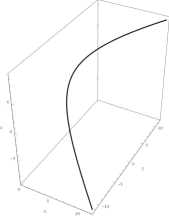
Figure 1. A hyperbolic cylindrical curve with $\tau_{0}=3$, $s\in(-\pi,\pi)$.

4. Timelike surfaces in $\mathbb{I}_{p}^{3}$

Let $M$ be a surface immersed in $\mathbb{I}_{p}^{3}$ without isotropic tangent planes. Then we call such a surface admissible. Let $T_{x}M$ be a non-isotropic tangent plane at a point $x\in M$. An admissible surface $M$ is said to be timelike (resp. lightlike) if the induced metric $g$ in $T_{x}M$ for each $x\in M$ from $\mathbb{I}_{p}^{3}$ is non-degenerate of index 1 (resp. degenerate).

Henceforth, we will not consider lightlike surfaces.

Assume that $M$ has a local parameterization in $\mathbb{I}_{p}^{3}$ as follows:

$$r:D\subseteq\mathbb{R}^{2}\longrightarrow\mathbb{I}_{p}^{3}:\text{ }\left(u_{1},u_{2}\right)\longmapsto\left(x\left(u_{1},u_{2}\right),y\left(u_{1},u_{2}\right),z\left(u_{1},u_{2}\right)\right)$$

for smooth real-valued functions $x,y,z$ on a domain $D\subseteq\mathbb{R}^{2}.$ Denote $\left(g_{ij}\right)$ the matrical expression of $g$ with respect to the basis $\left\{r_{u_{1}},r_{u_{2}}\right\}.$ Then we have

$$g_{ij}=\left\langle r_{u_{i}},r_{u_{j}}\right\rangle,\text{ }r_{u_{i}}=\frac{\partial r}{\partial u_{i}},\text{ }i,j=1,2.$$

It is easy to see that

$$\det\left(g_{ij}\right)=-\left(x_{u_{1}}y_{u_{2}}-x_{u_{2}}y_{u_{1}}\right)^{2}.$$

The unit normal vector field of $M$ is the isotropic vector $\xi=\left(0,0,1\right)$ since it is isotropically orthogonal to the tangent plane of $M$.

For the second fundamental form of $M$, we follow the similar way with Sachs (see [20], p. 155). Let $r\left(s\right)$ be an arc-length curve on $M$ and $T$ its tangent vector. We can take a side tangential vector $\sigma$ in $T_{x}M$ such that $\left\{T,\sigma\right\}$ is a positive oriented base. Therefore we have a decomposition:

$$r^{\prime\prime}=\frac{d^{2}r}{ds^{2}}=\kappa N=\kappa_{g}\sigma+\kappa_{n}\xi,$$

where $N$, $\kappa_{g}$ and $\kappa_{n}$ are the normal vector, geodesic and normal curvatures of $r$ on $M$, respectively. Put $\sigma=a_{1}r_{u_{1}}+a_{2}r_{u_{2}}.$ Due to $T=r_{u_{1}}\frac{du_{1}}{ds}+u_{2}\frac{du_{2}}{ds}$ and $\left\langle T,\sigma\right\rangle=0,$ we get

$$a_{1}=\theta\left(g_{12}\frac{du_{1}}{ds}+g_{22}\frac{du_{2}}{ds}\right),\text{ }a_{2}=-\theta\left(g_{11}\frac{du_{1}}{ds}+g_{12}\frac{du_{2}}{ds}\right),$$

where $\theta=\theta\left(u_{1},u_{2}\right)$ is some nonzero smooth function. Then we achieve

$$1=\det\left(\tilde{T},\tilde{\sigma}\right)=-\sqrt{\left|\det\left(g_{ij}\right)\right|}\theta$$

and hence

$$\sigma=-\frac{1}{\sqrt{\left|\det\left(g_{ij}\right)\right|}}\left[\left(g_{12}\frac{du_{1}}{ds}+g_{22}\frac{du_{2}}{ds}\right)r_{u_{1}}-\left(g_{11}\frac{du_{1}}{ds}+g_{12}\frac{du_{2}}{ds}\right)r_{u_{2}}\right].$$

Accordingly, we compute that

$$\left.\begin{array}[]{l}\kappa_{n}=\det\left(r^{\prime},\sigma,r^{\prime\prime}\right)=\dfrac{1}{\sqrt{\left|\det\left(g_{ij}\right)\right|}}\det\left(r_{u_{1}},r_{u_{2}},r^{\prime\prime}\right)\\ =\dfrac{1}{\sqrt{\left|\det\left(g_{ij}\right)\right|}}\sum\limits_{i,j=1}^{2}\det\left(r_{u_{1}},r_{u_{2}},r_{u_{i}u_{j}}\right)\left(\dfrac{du_{i}}{ds}\right)\left(\dfrac{du_{j}}{ds}\right),\end{array}\right.$$

which leads to the components of the second fundamental form given by

$$h_{ij}=\frac{\det\left(r_{u_{1}},r_{u_{2}},r_{u_{i}u_{j}}\right)}{\sqrt{\left|\det\left(g_{ij}\right)\right|}},\text{ }r_{u_{i}u_{j}}=\frac{\partial^{2}r}{\partial u_{i}\partial u_{j}},\text{ }i,j=1,2.$$

Thus the Gaussian curvature and the mean curvature of $M$ are respectively defined by

(4.1) $$K=\frac{\det\left(h_{ij}\right)}{\det\left(g_{ij}\right)}$$

and

(4.2) $$H=\frac{g_{11}h_{22}-2g_{12}h_{12}+g_{22}h_{11}}{2\det\left(g_{ij}\right)}.$$

By permutation of the coordinates, two different types of graph surfaces appear up to the absolute of $\mathbb{I}_{p}^{3}.$ For a graph of the function $u=u\left(x,y\right),$ the formulas (4.1) and (4.2) reduce to

$$K=-u_{xx}u_{yy}+\left(u_{xy}\right)^{2},\text{ }H=\frac{1}{2}\left(u_{xx}-u_{yy}\right).$$

Since the metric on the graph surface induced from $\mathbb{I}_{p}^{3}$ is $g=dx^{2}-dy^{2}$, it always becomes a flat surface. So, its Laplacian turns to

$$\bigtriangleup=\frac{\partial^{2}}{\partial u_{1}^{2}}-\frac{\partial^{2}}{\partial u_{2}^{2}}.$$

On the other side, the Gaussian and mean curvatures of the graph of $u=u\left(y,z\right)$ are given by

$$K=-\frac{u_{yy}u_{zz}-\left(u_{yz}\right)^{2}}{\left(u_{z}\right)^{4}},\text{ }H=\frac{\left(u_{z}\right)^{2}u_{yy}-2u_{y}u_{z}u_{yz}+\left(\left(u_{y}\right)^{2}-1\right)u_{zz}}{2\left(u_{z}\right)^{3}}.$$

5. Constant curvature surfaces of revolution in $\mathbb{I}_{p}^{3}$

Da Silva [8] provided via hyperbolic numbers that the pseudo isotropic motion given by $\bar{x}=px,$ $\bar{y}=\frac{1}{p}y,$ $p\neq 0$ is equivalent to the hyperpolic rotation (about $z-$axis) given by

(5.1) $$\bar{x}=x\cosh\theta+y\sinh\theta,\text{ }\bar{y}=x\sinh\theta+y\cosh\theta,$$

where $\theta\in\mathbb{R}.$

Let $u\longmapsto\left(u,0,f\left(u\right)\right)$ be a spacelike admissible curve lying in the isotropic $xz-$plane of $\mathbb{I}_{p}^{3}$ for a smooth function $f$. Rotating it around $z-$axis via hyperbolic rotations given by $\left(5.1\right)$ we derive

(5.2) $$r\left(u,v\right)=\left(u\cosh v,u\sinh v,f\left(u\right)\right).$$

We call the rotating curve profile curve. If the profile curve is a timelike curve $u\longmapsto\left(0,u,f\left(u\right)\right)$ lying in the isotropic $yz-$plane of $\mathbb{I}_{p}^{3}$, then rotating it around $\mathbf{z}-$axis yields

(5.3) $$r\left(u,v\right)=\left(u\sinh v,u\cosh v,f\left(u\right)\right).$$

The surfaces given by $\left(5.2\right)$ and $\left(5.3\right)$ are called surfaces of revolution in $\mathbb{I}_{p}^{3}.$ The Gaussian curvature of these surfaces in $\mathbb{I}_{p}^{3}$ is

(5.4) $$K=\frac{f^{\prime}f^{\prime\prime}}{u},$$

where $f^{\prime}\left(u\right)=\dfrac{df}{du},$ etc.

Now we assume that it has nonzero constant Gaussian curvature $K_{0}$ in $\mathbb{I}_{p}^{3}.$ Then $\left(5.4\right)$ can be rewritten as

(5.5) $$f^{\prime}=\sqrt{c_{1}+K_{0}u^{2}},c_{1}\in\mathbb{R}.$$

After integrating $\left(5.5\right),$ we obtain

$$f\left(u\right)=\frac{u}{2}\sqrt{c_{1}+K_{0}u^{2}}+\frac{c_{1}}{2\sqrt{K_{0}}}\ln\left(2K_{0}u+2\sqrt{K_{0}}\sqrt{c_{1}+K_{0}u^{2}}\right)+c_{2},\text{ }c_{2}\in\mathbb{R}$$

which implies the following result.

Theorem 5.1.

Let $M$ be a surface of revolution in $\mathbb{I}_{p}^{3}$ with nonzero constant Gaussian curvature $K_{0}.$ Then its profile curve is of the form $\left(u,0,f\left(u\right)\right)$, where

$$f\left(u\right)=\frac{u}{2}\psi\left(u\right)+\frac{c_{1}}{2\sqrt{K_{0}}}\ln\left|2\sqrt{K_{0}}\left(\sqrt{K_{0}}x+\psi\left(u\right)\right)\right|$$

for $\psi\left(u\right)=\sqrt{c_{1}+K_{0}u^{2}}$, $c_{1},c_{2}\in\mathbb{R}.$

We immediately have the following from $(5.4)$.

Corollary 5.1.

A surface of revolution is flat in $\mathbb{I}_{p}^{3}$ if and only if its profile curve is a non-isotropic line given by $\left(u,0,c_{1}u+c_{2}\right),$ $c_{1},c_{2}\in\mathbb{R}.$

The mean curvature $H$ of a surface of revolution $M$ in $\mathbb{I}_{p}^{3}$ is

(5.6) $$H=\frac{1}{2}\left(\frac{f^{\prime}}{u}+f^{\prime\prime}\right).$$

Assume that $M$ has constant mean curvature $H_{0}.$ After solving $\left(5.6\right)$ we deduce

$$f\left(u\right)=\frac{H_{0}}{2}u^{2}+c_{1}\ln u+c_{2},\text{ }c_{1},c_{2}\in\mathbb{R}.$$

Therefore we have proved the following results.

Theorem 5.2.

Let $M$ be a surface of revolution in $\mathbb{I}_{p}^{3}$ with constant mean curvature $H_{0}.$ Then its profile curve is of the form $\left(u,0,f\left(u\right)\right)$, where

$$f\left(u\right)=\frac{H_{0}}{2}u^{2}+c_{1}\ln u+c_{2},\text{ }c_{1},c_{2}\in\mathbb{R}.$$

Corollary 5.2.

A surface of revolution is minimal in $\mathbb{I}_{p}^{3}$ if and only if its profile curve is a non-isotropic curve given by $\left(u,0,c_{1}\ln u+c_{2}\right),$ $c_{1},c_{2}\in\mathbb{R}.$

Example 5.1.

Take the surfaces of revolution in $\mathbb{I}_{p}^{3}$ parameterized

$$r\left(u,v\right)=\left(u\cosh v,u\sinh v,u\right),\text{ }\left(u,v\right)\in\left[1,2\right]\times\left[0,1\right]$$

and

$$\left(u,v\right)=\left(u\cosh v,u\sinh v,\ln u+u^{2}\right),\text{ }\left(u,v\right)\in\left[1,2\right]\times\left[-1,1\right].$$

The above first surface is flat and the second is a constant mean curvature surface of revolution, $H=2.$ We plot these as in Figure 2 and Figure 3, respectively.

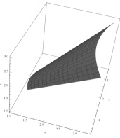
Figure 2. A flat surface of revolution, $K=0$.

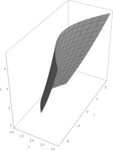
Figure 3. A constant curvature surface of revolution, $H=2$.

6. Surfaces of revolution with $H^{2}=K$ in $\mathbb{I}_{p}^{3}$

Next we aim to classify the surfaces of revolution given by (5.2) in $\mathbb{I}_{p}^{3}$ that satisfy $H^{2}=K$ which is the equality sign of the Euler inequality. For more generalizations of the famous inequality, see [4, 19, 20].

By considering the equalities $\left(5.4\right)$ and $\left(5.6\right),$ we have

(6.1) $$\frac{1}{4}\left(\left(\frac{f^{\prime}}{u}\right)^{2}+2\frac{f^{\prime}f^{\prime\prime}}{u}+\left(f^{\prime\prime}\right)^{2}\right)=\frac{f^{\prime}f^{\prime\prime}}{u}.$$

We can rewirte $\left(6.1\right)$ as

$$\left(\frac{f^{\prime}}{u}-f^{\prime\prime}\right)^{2}=0,$$

which implies

$$\frac{f^{\prime}}{u}-f^{\prime\prime}=0.$$

After solving this, we obtain

$$f\left(u\right)=c_{1}\frac{u^{2}}{2}+c_{2}$$

for $c_{1},c_{2}\in\mathbb{R}.$ By comparing (5.2) with (6.2) we see that the surface of revolution can be given in explicit form

(6.3) $$z=\frac{c_{1}}{2}\left(x^{2}-y^{2}\right)+c_{2},$$

which implies the following result.

Theorem 6.1.

The surfaces of revolution given by (5.2) in $\mathbb{I}_{p}^{3}$ with $H^{2}=K$ are only the spheres of parabolic type.

Example 6.1.

Consider the sphere of parabolic type in $\mathbb{I}_{p}^{3}$ given via $\left(6.3\right)$ such that $c_{1}=2$ and $c_{2}=0.$ Then its curvatures become $H=2$ and $K=4$. We plot it as in Figure 4.

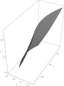
Figure 4. A surface of revolution with $H^{2}=K$.

7. Acknowlodgements

The figures in the present study were made by Wolfram Mathematica 11.0.

References

[1] M.E. Aydin, A Mihai, Ruled surfaces generated by elliptic
cylindrical curves in the isotropic space, Georgian Math. J., accepted for
publication.
[2] M.E. Aydin, I. Mihai, On certain surfaces in the isotropic
4-space, Math. Commun. 22(1) (2017), 41–51.
[3] M.E. Aydin, Classification results on surfaces in the isotropic 3-space, AKU J. Sci. Eng. 16 (2016), 239‐246.
[4] B. Y. Chen, Mean curvature and shape operator of isometric
immersions in real-space-forms, Glasg. Math. J. 38 (1996), 87–97.
[5] B. Y. Chen, S. Decu, L. Verstraelen, Notes on isotropic geometry
of production models, Kragujevac J. Math. 38(1) (2014), 23–33.
[6] B. Y. Chen, Pseudo-Riemannian geometry, -Invariants and
applications, World Scientific, Singapore, 2011.
[7] M. Crasmareanu, Cylindrical Tzitzeica curves implies forced
harmonic oscillators, Balkan J. Geom. Appl., 7(1) (2002), 37-42.
[8] L.C.B. Da Silva, Rotation minimizing frames and spherical curves
in simply isotropic and semi-isotropic 3-spaces, arXiv:1707.06321 [math.DG].
[9] B. Divjak, Geometrija pseudogalilejevih prostora (Ph.D. thesis),
University of Zagreb, 1997.
[10] B. Divjak, Curves in pseudo-Galilean geometry, Annales
Universitatis Scientiarum Budapestinensis de Rolando Eötvös
Nominatae 41 (1998), 117–128.
[11] Z. Erjavec, B. Divjak, D. Horvat, The general solutions of
Frenet’s system in the equiform geometry of the Galilean, pseudo-Galilean,
simple isotropic and double isotropic space, Int. Math. Forum 6(17) (2011),
837-856.
[12] O. Giering, Vorlesungen über höhere Geometrie, Friedr.
Vieweg & Sohn, Braunschweig, Germany, 1982.
[13] M. Husty, O. Röschel, On a particular class of cyclides in
isotropic respectively pseudoisotropic space, Coll. Math. Soc. J. Bolyai 46
(1984), 531–557.
[14] M.K. Karacan, D.W. Yoon, S. Kiziltug, Helicoidal surfaces in the three dimensional
simply isotropic space , Tamkang J. Math. 48 (2017), 123–134.
[15] D. Klawitter, Clifford Algebras: Geometric Modelling and Chain
Geometries with Application in Kinematics, Springer Spektrum, 2015.
[16] R. Lopez, Differential Geometry of curves and surfaces in
Lorentz-Minkowski space, Int. Electron. J. Geom. 7 (2014), 44-107.
[17] F. Meszaros, Die Zykliden 3. Ordnung im pseudoisotropen Raum
II,, Math. Pannonica 4(2) (1993), 273-285.
[18] F. Meszaros, Klassifikationstheorie der verallgemeinerten
zykliden 4. ordnung in pseudoisotropen Raum, Math. Pannonica 18(2) (2007),
299-323.
[19] A. Mihai, Geometric inequalities for purely real submanifolds
in complex space forms, Results Math. 55 (2009), 457–468.
[20] I. Mihai, On the generalized Wintgen inequality for Lagrangian
submanifolds in complex space forms, Nonlinear Analysis 95 (2014), 714-720.
[21] Z. Milin-Sipus, B. Divjak, Surfaces of constant curvature in
the pseudo-Galilean space, Int. J. Math. Sci., 2012, Art ID375264, 28pp.
[22] Z. Milin-Sipus, Translation surfaces of constant curvatures in
a simply isotropic space, Period. Math. Hung. 68 (2014), 160-175
[23] A.O. Ogrenmis, Rotational surfaces in isotropic spaces
satisfying Weingarten conditions, Open Physics 14(9) (2016), 221–225.
[24] B. O‘Neill, Semi-Riemannian geometry with applications to
relativity, Academic Press, New York, 1983.
[25] A. Onishchick, R. Sulanke, Projective and Cayley-Klein
Geometries, Springer, 2006.
[26] H. Sachs, Isotrope Geometrie des Raumes, Vieweg Verlag,
Braunschweig, 1990.
[27] K. Strubecker, Differentialgeometrie des isotropen Raumes III,
Flachentheorie, Math. Zeitsch. 48 (1942), 369-427.
[28] I. M. Yaglom, A simple non-Euclidean Geometry and Its Physical
Basis, An elementary account of Galilean geometry and the Galilean principle
of relativity, Heidelberg Science Library. Translated from the Russian by
Abe Shenitzer. With the editorial assistance of Basil Gordon.
Springer-Verlag, New York-Heidelberg, 1979.