Exact Solutions and Conserved Quantities in $f(R,T)$ Gravity

Abstract

This paper explores Noether and Noether gauge symmetries of anisotropic universe model in $f(R,T)$ gravity. We consider two particular models of this gravity and evaluate their symmetry generators as well as associated conserved quantities. We also find exact solution by using cyclic variable and investigate its behavior via cosmological parameters. The behavior of cosmological parameters turns out to be consistent with recent observations which indicates accelerated expansion of the universe. Next we study Noether gauge symmetry and corresponding conserved quantities for both isotropic and anisotropic universe models. We conclude that symmetry generators and the associated conserved quantities appear in all cases.

Keywords: Noether symmetry; Conserved quantity; $f(R,T)$ gravity.
PACS: 04.20.Jb; 04.50.Kd; 95.36.+x.

1 Introduction

In the last century, the crucial observational discoveries established revolutionary advancements in modern cosmology that introduced a new vision of the current accelerated expanding universe. The accelerated epoch of the universe known as “dark energy” (DE) possesses a huge amount of negative pressure. At theoretical level, the conclusive evidences about accelerated expansion of the universe and enigmatic behavior of DE lead to introduce modified theories of gravity. The $f(R)$ gravity is the simplest proposal ($R$ represents Ricci scalar) developed by replacing $R$ with a generic function independent of any non-minimal curvature and matter coupling in the Einstein-Hilbert action.

Different researchers established basic review of $f(R)$ gravity [1] and also discussed stability of its different models [2]. The idea of coupling between curvature and matter was initially presented by Nojiri and Odintsov [3] who explored explicit and implicit couplings in $f(R)$ gravity. Harko et al. [4] developed a gravitational theory involving both curvature as well as matter components known as $f(R,T)$ gravity ($T$ denotes trace of the energy-momentum tensor). Sharif and Zubair [5] discussed universe evolution via energy conditions along with stability criteria, reconstructed different DE models, exact solutions of anisotropic universe and thermodynamical picture in $f(R,T)$ gravity.

The discovery of CMBR reveals that the early universe was spatially homogeneous but largely anisotropic while this anisotropy still exists in terms of CMB temperature in the present universe. We consider Bianchi type models which measure the effect of anisotropy in the early universe through current observations [6]. The anisotropic universe model indicates that the initial anisotropy determines the fate of rapid expansion of the early universe which will continue for initially large values of anisotropy. If the initial anisotropy is small then the rapid expansion will end leading to a highly isotropic universe [7]. Akarsu and Kilinc [8] studied Bianchi type I (BI) model that corresponds to de Sitter universe for different equation of state (EoS) models. Sharif and Zubair [9] formulated exact solutions of BI universe model for power-law and exponential expansions in $f(R,T)$ gravity. Shamir [10] discussed exact solutions of locally rotationally symmetric (LRS) BI universe model and investigated physical behavior of cosmological parameters in this gravity. Kanakavalli and Ananda [11] obtained exact solutions of LRS BI model in the presence of cosmic string source and curvature-matter coupling.

Symmetry approximation plays a crucial role to determine exact solutions or elegantly reduces complexity of a non-linear system of equations. Noether symmetry is a useful approach to evaluate unknown parameters of differential equations. Sharif and Waheed explored Bardeen model [12] as well as stringy charged black holes [13] via approximate symmetry. They also evaluated Noether symmetries of FRW and LRS BI models by including an inverse curvature term in the action of Brans-Dicke theory [14]. Kucukakca et al. [15] established exact solutions of LRS BI universe model through Noether symmetry approach in the same gravity. Jamil et al. [16] discussed Noether symmetry in $f(\mathcal{T})$ gravity ($\mathcal{T}$ denotes torsion) that involves matter as well as scalar field contributions and determined explicit form of $f(\mathcal{T})$ for quintessence and phantom models. Kucukakca [17] found exact solutions of flat FRW universe model via Noether symmetry in scalar-tensor theory incorporating non-minimal coupling with torsion scalar. Sharif and Shafique [18] discussed Noether and Noether gauge symmetries in this gravity. Sharif and Fatima [19] explored Noether symmetry of flat FRW model through vacuum and non-vacuum cases in $f(G)$ gravity.

Capozziello et al. [20] explored Noether symmetry to determine exact solutions of spherically symmetric spacetime in $f(R)$ gravity. Vakili [21] obtained Noether symmetry of flat FRW metric and analyzed the behavior of effective EoS parameter in quintessence phase. Jamil et al. [22] studied Noether symmetry of flat FRW universe using tachyon model in this gravity. Hussain et al. [23] studied Noether gauge symmetry of flat FRW universe model for $f(R)$ power-law model which generates zero gauge term. Shamir et al. [24] analyzed Noether gauge symmetry for the same model as well as for static spherically symmetric spacetime and found non-zero gauge term. Kucukakca and Camci [25] established Noether gauge symmetry of FRW universe model in Palatini formalism of $f(R)$ gravity. Momeni et al. [26] investigated the existence of Noether symmetry and discussed stability of solutions for flat FRW universe model in $f(R,T)$ and mimetic $f(R)$ gravity. They also explored a class of solutions with future singularities.

In this paper, we discuss Noether and Noether gauge symmetries of BI universe model in $f(R,T)$ gravity. We formulate exact solution of the field equations to discuss cosmic evolution via cosmological parameters. The format of this paper is as follows. In section 2, we discuss a basic formalism of $f(R,T)$ gravity, Noether and Noether gauge symmetries. Section 3 explores Noether symmetry of BI model for two theoretical models of $f(R,T)$ gravity and also establish exact solution via cyclic variables. In section 4, we obtain symmetry generator and corresponding conserved quantities through Noether gauge symmetry for flat FRW and BI models. In the last section, we summarize the results.

2 Basic Framework

The current cosmic expansion successfully discusses not only from the contribution of the scalar-curvature part but also describes from a non-minimal coupling between curvature and matter components as well. This non-minimal coupling yields non-zero divergence of the energy-momentum tensor due to which an extra force appears that deviates massive test particles from geodesic trajectories. The action of such modified gravity is given by [4]

$$\mathcal{I}=\int d^{4}x\sqrt{-g}[\frac{f(R,T)}{2\kappa^{2}}+\mathcal{L}_{m}],$$ (1)

where $f$ describes a simple coupling of geometry and matter whereas $\mathcal{L}_{m}$ denotes the matter Lagrangian. The variation of action (1) with respect to $g_{\mu\nu}$ yields non-linear partial differential equation of the following form

$$f_{R}(R,T)R_{\mu\nu}-\frac{1}{2}f(R,T)g_{\mu\nu}+(g_{\mu\nu}\Box-\nabla_{\mu}\nabla_{\nu})f_{R}(R,T)+f_{T}(R,T)T_{\mu\nu}$$

$$+f_{T}(R,T)\Theta_{\mu\nu}=\kappa^{2}T_{\mu\nu},$$ (2)

where $\nabla_{\mu}$ shows covariant derivative and

$$\Box = \nabla_{\mu}\nabla^{\mu},\quad f_{R}(R,T)=\frac{\partial f(R,T)}{\partial R},\quad f_{T}(R,T)=\frac{\partial f(R,T)}{\partial T},$$

$$\Theta_{\mu\nu} = \frac{g^{\alpha\beta}\delta T_{\alpha\beta}}{\delta g^{\mu\nu}}=g_{\mu\nu}\mathcal{L}_{m}-2T_{\mu\nu}-2g^{\alpha\beta}\frac{\partial^{2}\mathcal{L}_{m}}{\partial g^{\alpha\beta}\partial g^{\mu\nu}}.$$

The trace of Eq.(2) provides a significant relationship between geometric and matter parts as follows

$$Rf_{R}(R,T)+3\Box f_{R}(R,T)-2f(R,T)+Tf_{T}(R,T)+\Theta f_{T}(R,T)=\kappa^{2}T.$$

Harko et al [4] introduced some theoretical models for different choices of matter as

• $f(R,T)$=$R+2f(T)$,

• $f(R,T)$=$f_{1}(R)+f_{2}(T)$,

• $f(R,T)$=$f_{1}(R)+f_{2}(R)f_{3}(T)$.

Noether symmetry is the most significant approach to deal with non-linear partial differential equations. The existence of Noether symmetry is possible only if Lie derivative of Lagrangian vanishes, i.e., the vector field is unique on the tangent space. In such situation, the vector field behaves as a symmetry generator which further generates conserved quantity. Noether gauge symmetry being generaliztion of Noether symmetry preserves some extra symmetries along a non-vanishing gauge term. The vector field and its first order prolongation are defined as

$$K = \xi(t,q^{i})\frac{\partial}{\partial t}+\eta^{j}(t,q^{i})\frac{\partial}{\partial q^{j}},$$

$$K^{[1]} = K+(\eta^{j},_{t}+\eta^{j},_{i}\dot{q}^{i}-\xi,_{t}\dot{q}^{j}-\xi,_{i}\dot{q}^{i}\dot{q}^{j})\frac{\partial}{\partial\dot{q}^{i}},$$

where $t$ identifies as affine parameter, $\xi,~{}\eta$ are symmetry generator coefficients, $q^{i}$ represents $n$ generalized positions and dot denotes time derivative. The vector field $K$ generates Noether gauge symmetry if Lagrangian preserves the following condition

$$K^{[1]}\mathcal{L}+(D\xi)\mathcal{L}=DG(t,q^{i}).$$

Here $G(t,q^{i})$ represents the gauge term and $D$ denotes the total derivative operator defined as

$$D = \frac{\partial}{\partial t}+\dot{q}^{i}\frac{\partial}{\partial q^{i}}.$$

According to Noether theorem, there exists a conserved quantity corresponding to each symmetry of a system. In case of Noether gauge symmetry, the conserved quantity for vector field $K$ takes the form

$$\Sigma=G-\xi\mathcal{L}-(\eta^{j}-\dot{q}^{j}\xi)\frac{\partial\mathcal{L}}{\partial\dot{q}^{j}}.$$

For the existence of Noether symmetry, the following condition must holds

$$L_{K}\mathcal{L}=K\mathcal{L}=0,$$

where $L$ represents Lie derivative while the vector field $K$ and conserved quantity corresponding to symmetry generator turn out to be

$$K=\beta^{i}(q^{i})\frac{\partial}{\partial q^{i}}+\left[\frac{d}{dt}(\beta^{i}(q^{i}))\right]\frac{\partial}{\partial\dot{q}^{i}},\quad\Sigma=-\eta^{j}\frac{\partial\mathcal{L}}{\partial\dot{q}^{j}}.$$ (3)

The equation of motion and associated Hamiltonian equation of a dynamical system are defined as

$$\frac{\partial\mathcal{L}}{\partial q^{i}}-\frac{d}{dt}\left(\frac{\partial\mathcal{L}}{\partial\dot{q}^{i}}\right)=0,\quad\Sigma_{i}\dot{q}^{i}p_{i}-\mathcal{L}=\mathcal{H},\quad p_{i}=\frac{\partial\mathcal{L}}{\partial q^{i}},$$

where $p_{i}$ represents conjugate momenta of configuration space.

3 Noether Symmetry for BI Universe Model

Here we apply Noether symmetry approach to deal with non-linear partial differential equation (2) and evaluate symmetry generators as well as corresponding conserved quantities of BI universe model given by

$$ds^{2}=-dt^{2}+a^{2}(t)dx^{2}+b^{2}(t)(dy^{2}+dz^{2}),$$ (4)

where $t$ denotes cosmic time, scale factors $a$ and $b$ measure expansion of the universe in $x$ and $y,~{}z$-directions, respectively. We consider the perfect fluid distribution given by

$$T_{\mu\nu}=(\rho+p)u_{\mu}u_{\nu}+pg_{\mu\nu},$$

where $p,~{}\rho$ and $u_{\mu}$ represent pressure, energy density and four-velocity of the fluid, respectively. To evaluate the Lagrangian, we rewrite the action (1) as

$$\mathcal{I}=\int\sqrt{-g}[f(R,T)-\lambda(R-\bar{R})-\chi(T-\bar{T})+\mathcal{L}_{m}]dt,$$ (5)

where $\sqrt{-g}=ab^{2}$, $\bar{R},~{}\bar{T}$ are dynamical constraints while $\lambda,~{}\chi$ are Lagrange multipliers given by

$$\bar{R}=\frac{2}{ab^{2}}(\ddot{a}b^{2}+2ab\ddot{b}+2b\dot{a}\dot{b}+a\dot{b^{2}}),\quad\bar{T}=3p(a,b)-\rho(a,b),$$

$$\lambda=f_{R}(R,T),\quad\chi=f_{T}(R,T).$$

The field equation (2) is not easy to tackle with perfect fluid configuration and also there is no unique definition of matter Lagrangian. In order to construct Lagrangian, we consider $\mathcal{L}_{m}=p(a,b)$ which yields

$$\mathcal{L}(a,b,R,T,\dot{a},\dot{b},\dot{R},\dot{T})=ab^{2}[f(R,T)-Rf_{R}(R,T)-Tf_{T}(R,T)$$

$$+f_{T}(R,T)(3p(a,b)-\rho(a,b))+p(a,b)]-(4b\dot{a}\dot{b}+2a\dot{b}^{2})f_{R}(R,T)$$

$$-(2b^{2}\dot{a}\dot{R}+4ab\dot{b}\dot{R})f_{RR}(R,T)-(2b^{2}\dot{a}\dot{T}+4ab\dot{b}\dot{T})f_{RT}(R,T).$$ (6)

The corresponding equations of motion and energy function of dynamical system become

$$\frac{\dot{b^{2}}}{b^{2}}+\frac{2\ddot{b}}{b}=-\frac{1}{2f_{R}(R,T)}[f(R,T)-Rf_{R}(R,T)-Tf_{T}(R,T)+f_{T}(R,T)$$

$$\times(3p(a,b)-\rho(a,b))+p(a,b)+a\{f_{T}(3p,_{{}_{a}}-\rho,_{{}_{a}})+p,_{{}_{a}}\}+\frac{4\dot{b}\dot{R}f_{RR}(R,T)}{b}$$

$$+2\ddot{R}f_{RR}(R,T)+2\dot{R}^{2}f_{RRR}(R,T)+4\dot{R}\dot{T}f_{RRT}(R,T)+2\ddot{T}f_{RT}(R,T)$$

$$+2\dot{T}^{2}f_{RTT}(R,T)],$$ (7)

$$\frac{\ddot{a}}{a}+\frac{\dot{a}\dot{b}}{ab}+\frac{\ddot{b}}{b}=-\frac{1}{4f_{R}(R,T)}[2(f(R,T)-Rf_{R}(R,T)-Tf_{T}(R,T)$$

$$+f_{T}(R,T)(3p(a,b)-\rho(a,b))+p(a,b))+b\{f_{T}(3p,_{{}_{b}}-\rho,_{{}_{b}})+p,_{{}_{b}}\}]$$

$$+2(a^{-1}\dot{a}\dot{R}+\ddot{R})f_{RR}+2\dot{R}^{2}f_{RRR}+2(a^{-1}\dot{a}\dot{T}+\ddot{T})f_{RT}+2(b^{-1}\dot{b}\dot{R}+2\dot{R}\dot{T}$$

$$+\dot{T}^{2})f_{RRT}+2b^{-1}\dot{b}\dot{T}f_{RTT}=0,$$ (8)

$$\frac{\dot{b^{2}}}{b^{2}}+\frac{2\dot{a}\dot{b}}{ab}=-\frac{1}{f_{R}(R,T)}\left[\left(\frac{2\dot{b}\dot{R}}{b}+\frac{\dot{a}\dot{R}}{a}\right)f_{RR}(R,T)+\left(\frac{2\dot{b}\dot{T}}{b}+\frac{\dot{a}\dot{T}}{a}\right)\right.$$

$$\times\left.f_{RT}(R,T)+\frac{1}{2}(f(R,T)-Rf_{R}(R,T)-Tf_{T}(R,T)+f_{T}(R,T)(3p(a,b)\right.$$

$$\left.-\rho(a,b))+p(a,b))\right].$$ (9)

The conjugate momenta corresponding to configuration space ($a,~{}b,~{}R,~{}T$) are

$$p_{a} = \frac{\partial\mathcal{L}}{\partial\dot{a}}=-4b\dot{b}f_{R}(R,T)-2b^{2}(\dot{R}f_{RR}(R,T)+\dot{T}f_{RT}(R,T)),$$ (10)

$$p_{b} = \frac{\partial\mathcal{L}}{\partial\dot{b}}=-4f_{R}(R,T)(a\dot{b}+b\dot{a}-4ab(\dot{R}f_{RR}(R,T)+\dot{T}f_{RT}(R,T)),$$ (11)

$$p_{R} = \frac{\partial\mathcal{L}}{\partial\dot{R}}=-(4ab\dot{b}+2b^{2}\dot{a})f_{RR}(R,T),$$ (12)

$$p_{T} = \frac{\partial\mathcal{L}}{\partial\dot{T}}=-(4ab\dot{b}+2b^{2}\dot{a})f_{RT}(R,T).$$ (13)

For Noether symmetry, the vector field (3) takes the following form

$$K=\alpha\frac{\partial}{\partial a}+\beta\frac{\partial}{\partial b}+\gamma\frac{\partial}{\partial R}+\delta\frac{\partial}{\partial T}+\dot{\alpha}\frac{\partial}{\partial\dot{a}}+\dot{\beta}\frac{\partial}{\partial\dot{b}}+\dot{\gamma}\frac{\partial}{\partial\dot{R}}+\dot{\delta}\frac{\partial}{\partial\dot{T}},$$ (14)

where $\alpha,~{}\beta,~{}\gamma$ and $\delta$ are unknown coefficients of generator which depend on variables $a,~{}b,~{}R$ and $T$ while the time derivatives of these coefficients are

$$\dot{\alpha} = \dot{a}\frac{\partial\alpha}{\partial a}+\dot{b}\frac{\partial\alpha}{\partial b}+\dot{R}\frac{\partial\alpha}{\partial R}+\dot{T}\frac{\partial\alpha}{\partial T},\quad\dot{\beta}=\dot{a}\frac{\partial\beta}{\partial a}+\dot{b}\frac{\partial\beta}{\partial b}+\dot{R}\frac{\partial\beta}{\partial R}+\dot{T}\frac{\partial\beta}{\partial T},$$

$$\dot{\gamma} = \dot{a}\frac{\partial\gamma}{\partial a}+\dot{b}\frac{\partial\gamma}{\partial b}+\dot{R}\frac{\partial\gamma}{\partial R}+\dot{T}\frac{\partial\gamma}{\partial T},\quad\dot{\delta}=\dot{a}\frac{\partial\delta}{\partial a}+\dot{b}\frac{\partial\delta}{\partial b}+\dot{R}\frac{\partial\delta}{\partial R}+\dot{T}\frac{\partial\delta}{\partial T}.$$ (16)

Taking Lie derivative of Lagrangian (6) for vector field (14) and inserting Eqs.(LABEL:7) and (16), we obtain the following over determined system of equations by comparing the coefficients of $\dot{a}^{2},~{}\dot{b}^{2},~{}\dot{R}^{2},~{}\dot{T}^{2},~{}\dot{a}\dot{b},~{}\dot{a}\dot{R},~{}\dot{a}\dot{T},~{}\dot{b}\dot{R},~{}\dot{b}\dot{T}$ and $\dot{R}\dot{T}$ as

$$(b\alpha,_{{}_{R}}+2a\beta,_{{}_{R}})f_{RR}=0,$$ (17)

$$(b\alpha,_{{}_{T}}+2a\beta,_{{}_{T}})f_{RT}=0,$$ (18)

$$2\beta,_{{}_{a}}f_{R}+b\gamma,_{{}_{a}}f_{RR}+b\delta,_{{}_{a}}f_{RT}=0,$$ (19)

$$b\alpha,_{{}_{R}}f_{RT}+b\alpha,_{{}_{T}}f_{RR}+2a\beta,_{{}_{R}}f_{RT}+2a\beta,_{{}_{T}}f_{RR}=0,$$ (20)

$$2\beta f_{RR}+b\gamma f_{RRR}+b\delta f_{RRT}+b\alpha,_{{}_{a}}f_{RR}+2a\beta,_{{}_{a}}f_{RR}+2\beta,_{{}_{R}}f_{R}+b\gamma,_{{}_{R}}f_{RR}$$

$$+b\delta,_{{}_{R}}f_{RT}=0,$$ (21)

$$2\beta f_{RT}+b\gamma f_{RRT}+b\delta f_{RTT}+b\alpha,_{{}_{a}}f_{RT}+2a\beta,_{{}_{a}}f_{RT}+2\beta,_{{}_{T}}f_{R}+b\gamma,_{{}_{T}}f_{RR}$$

$$+b\delta,_{{}_{T}}f_{RT}=0,$$ (22)

$$2\beta f_{R}+2b\gamma f_{RR}+2b\delta f_{RT}+2b\alpha,_{{}_{a}}f_{R}+2a\beta,_{{}_{a}}f_{R}+2b\beta,_{{}_{b}}f_{R}+2ab\gamma,_{{}_{a}}f_{RR}$$

$$+b^{2}\gamma,_{{}_{b}}f_{RR}+2ab\delta,_{{}_{a}}f_{RT}+b^{2}\delta,_{{}_{b}}f_{RT}=0,$$ (23)

$$2b\alpha f_{RR}+2a\beta f_{RR}+2ab\gamma f_{RRR}+2ab\delta f_{RRT}+b^{2}\alpha,_{{}_{b}}f_{RR}+2b\alpha,_{{}_{R}}f_{R}+2ab$$

$$\times\beta,_{{}_{b}}f_{RR}+2a\beta,_{{}_{R}}f_{R}+2ab\gamma,_{{}_{R}}f_{RR}+2ab\delta,_{{}_{R}}f_{RT}=0,$$ (24)

$$2b\alpha f_{RT}+2a\beta f_{RT}+2ab\gamma f_{RRT}+2ab\delta f_{RTT}+b^{2}\alpha,_{{}_{b}}f_{RT}+2b\alpha,_{{}_{T}}f_{R}+2ab$$

$$\times\beta,_{{}_{b}}f_{RT}+2a\beta,_{{}_{T}}f_{R}+2ab\gamma,_{{}_{T}}f_{RR}+2ab\delta,_{{}_{T}}f_{RT}=0,$$ (25)

$$\alpha f_{R}+a\gamma f_{RR}+a\delta f_{RT}+2b\alpha,_{{}_{b}}f_{R}+2a\beta,_{{}_{b}}f_{R}+2ab\gamma,_{{}_{b}}f_{RR}+2ab\delta,_{{}_{b}}$$

$$\times f_{RT}=0,$$ (26)

$$b^{2}\alpha[f-Rf_{R}-Tf_{T}+f_{T}(3p-\rho)+p+a\{f_{T}(3p,_{{}_{a}}-\rho,_{{}_{a}})+p,_{{}_{a}}\}]+\beta[2ab$$

$$\times(f-Rf_{R}-Tf_{T}+f_{T}(3p-\rho)+p)+ab^{2}\{f_{T}(3p,_{{}_{b}}-\rho,_{{}_{b}})+p,_{{}_{b}}\}]+ab^{2}$$

$$\times\gamma[-(Rf_{RR}+Tf_{RT})+f_{RT}(3p-\rho)]+ab^{2}\delta[-(Rf_{RT}+Tf_{TT})+f_{TT}$$

$$\times(3p-\rho)]=0.$$ (27)

We solve this non-linear system of partial differential equations for two models of $f(R,T)$ gravity and evaluate possible solutions of symmetry generator coefficients as well as corresponding conserved quantities.

3.1 $f(R,T)=R+2f(T)$

Here we discuss a solution for a simple model that explores Einstein gravity with matter components such as $f(R,T)=R+2f(T)$, where the curvature term behaves as a leading term of the model. This model corresponds to $\Lambda$CDM model when matter part comprises cosmological constant as a function of trace $T$. Consequently, this model reduces to

$$f(R,T)=R+2\Lambda+h(T).$$ (28)

To find the solution of Eqs.(17)-(27), we consider power-law form of unknown coefficients of vector field as

$$\alpha = \alpha_{0}a^{\alpha_{1}}b^{\alpha_{2}}R^{\alpha_{3}}T^{\alpha_{4}},\quad\beta=\beta_{0}a^{\beta_{1}}b^{\beta_{2}}R^{\beta_{3}}T^{\beta_{4}},$$ (29)

$$\gamma = \gamma_{0}a^{\gamma_{1}}b^{\gamma_{2}}R^{\gamma_{3}}T^{\gamma_{4}},\quad\delta=\delta_{0}a^{\delta_{1}}b^{\delta_{2}}R^{\delta_{3}}T^{\delta_{4}},$$ (30)

where the powers are unknown constants to be determined. Using these coefficients in Eqs.(17)-(25), we obtain

$$\alpha_{0} = -\beta_{0}(\alpha_{2}+2),\quad\alpha_{1}=1,\quad\alpha_{3}=0,\quad\alpha_{4}=0,\quad\gamma=0,$$

$$\beta_{1} = 0,\quad\beta_{2}=\alpha_{2}+1,\quad\beta_{3}=0,\quad\beta_{4}=0.$$

Inserting these values in Eq.(29), it follows that

$$\alpha=-\beta_{0}(\alpha_{2}+2)ab^{\alpha_{2}},\quad\beta=\beta_{0}b^{\alpha_{2}+1}.$$

In order to evaluate $\alpha_{2}$, we substitute these solutions in Eq.(26) which implies that either $\alpha_{2}=0$ or $\alpha_{2}=\frac{1}{2}$.

Case I: $\alpha_{2}=0$

In this case, the generator coefficients turn out to be

$$\alpha=-2\beta_{0}a,\quad\beta=\beta_{0}b.$$

In order to evaluate the remaining coefficients, we insert these values in Eqs.(7), (9) and (27) which give

$$h(T) = l_{1}T+l_{2},\quad\delta=0,\quad p=l_{3}a^{-\frac{1}{5}}b^{-\frac{2}{5}},$$

$$\rho = -\frac{1}{2l_{1}}[2\Lambda+l_{2}+(3l_{1}-1)l_{3}a^{-\frac{1}{5}}b^{-\frac{2}{5}}].$$

Substituting all these solutions in Eqs.(17)-(25), we obtain $l_{1}=-\frac{19}{3}$. Consequently, the coefficients of symmetry generator and $f(R,T)$ model become

$$\alpha=-2\beta_{0}a,\quad\beta=\beta_{0}b,\quad\gamma=0,\quad\delta=0,\quad f(R,T)=R-\frac{19T}{3},$$

where $h(T)=-\frac{19T}{3}-2\Lambda$ and $T=\frac{87}{19}l_{3}a^{-\frac{1}{5}}b^{-\frac{2}{5}}$. To avoid Dolgov-Kawasaki instability, the $f(R,T)$ model preserves the following conditions [27]

$$f_{R}(R)>0,\quad f_{RR}(R)>0,\quad 1+f_{T}(R,T)>0,\quad R>R_{0}.$$ (31)

In this case, the constructed $f(R,T)$ model is found to be viable for $l_{3}<0$. Using the values of symmetry generator coefficients, we obtain symmetry generator which yields scaling symmetry and its conserved quantity as

$$K=-2\beta_{0}a\frac{\partial}{\partial a}+\beta_{0}b\frac{\partial}{\partial b},\quad\Sigma=\beta_{0}[-4ab\dot{b}+4\dot{a}b^{2}].$$

Now we solve the field equations using cyclic variable whose existence is assured by the presence of symmetry generator of Noether symmetry. We consider a point transformation which reduces complex nature of the system to $\phi:(a,b)\rightarrow(v,z)$ implying that $\phi_{K}dv=0$ and $\phi_{K}dz=1$. The second mapping indicates that the Lagrangian must be free from the variable $z$. Imposing this point transformation, we reduce the complexity of the system as

$$v=\zeta_{0}a^{\frac{1}{2}}b,\quad z=\frac{\ln b}{\beta_{0}},$$ (32)

where $z$ is cyclic variable and $\zeta_{0}$ denotes arbitrary constant. The inverse point transformation of variables yields

$$a=\zeta_{1}v^{\frac{1}{2}}e^{-2\beta_{0}z},\quad b=\zeta_{2}e^{\beta_{0}z},\quad\rho=-\frac{30\zeta_{3}v^{-\frac{2}{5}}}{19},\quad p=\zeta_{3}v^{-\frac{2}{5}}.$$ (33)

Here we redefine arbitrary constants as $\zeta_{3}=l_{3}\zeta_{1}^{-\frac{1}{5}}\zeta_{2}^{-\frac{2}{5}}$. For the above solutions, the Lagrangian (6) and the corresponding equations of motion with associated energy function (7)-(9) take the form

$$\mathcal{L}=\zeta_{4}(4\beta_{0}v^{\frac{-1}{2}}\dot{v}\dot{z}+4\beta_{0}^{2}v^{\frac{1}{2}}\dot{z}^{2}-30v^{\frac{2}{5}}),$$

$$2\beta_{0}v^{\frac{-1}{2}}\ddot{z}+2\beta_{0}^{2}v^{-\frac{1}{2}}\dot{z}^{2}-12v^{-\frac{3}{5}}=0,$$

$$8\beta_{0}v^{\frac{1}{2}}\ddot{z}+v^{-\frac{3}{2}}\dot{v}^{2}+4\beta_{0}v^{-\frac{1}{2}}\dot{z}-2v^{-\frac{1}{2}}\ddot{v}=0,$$

$$30v^{\frac{2}{5}}+4\beta_{0}^{2}v^{\frac{1}{2}}\dot{z}^{2}+\beta_{0}v^{-\frac{3}{2}}\dot{v}^{2}\dot{z}-2\beta_{0}v^{-\frac{1}{2}}\dot{v}\ddot{z}=0.$$

We solve the above equations to evaluate the time dependent solutions of new variables ($v,~{}z$)

$$v=2(t-\zeta_{4})^{\frac{1}{2}}(t^{2}-2t+\zeta_{4}^{2}),\quad z=\frac{1}{12\beta_{0}}[12\beta_{0}\zeta_{5}-2.93-4\ln[(t-\zeta_{4})^{\frac{5}{2}}]],$$

where $\zeta_{4}$ and $\zeta_{5}$ represent integration constants. Inserting these values into Eq.(33), we obtain

$$a = \frac{8}{5}\zeta_{1}e^{-2\beta_{0}\zeta_{5}}(t-\zeta_{4})^{\frac{5}{3}},\quad b=\frac{8}{5}\zeta_{2}e^{\beta_{0}\zeta_{5}}(t-\zeta_{4})^{-\frac{1}{3}}(t^{2}-2t\zeta_{1}+\zeta_{1}^{2}),$$ (34)

$$\rho = -\frac{30\zeta_{3}}{19}[2(t-\zeta_{4})^{\frac{1}{2}}(t^{2}-2t+\zeta_{4}^{2})]^{-\frac{2}{5}},\quad p=\zeta_{3}[2(t-\zeta_{4})^{\frac{1}{2}}(t^{2}-2t+\zeta_{4}^{2})]^{-\frac{2}{5}}.$$

We study the behavior of some well-known cosmological parameters like Hubble, deceleration and EoS parameters using scale factors and matter contents. These parameters play significant role to discuss cosmic expansion as Hubble parameter $(H)$ measures the rate of cosmic expansion while deceleration parameter $(q)$ determines that either expansion is accelerated $(q<0)$ or decelerated $(q>0)$ or constant expansion ($q=0$). The EoS parameter $(\omega=\frac{p}{\rho})$ evaluates different eras of the universe and also differentiates DE era into different phases like quintessence ($-1<\omega\leq-1/3$) or phantom ($\omega<-1$). In case of BI universe model, the Hubble and deceleration parameters are

$$H=\frac{1}{3}\left(\frac{\dot{a}}{a}+\frac{2\dot{b}}{b}\right),\quad q=-\frac{\dot{H}}{H^{2}}-1.$$

Using Eq.(34), the Hubble and deceleration parameters turn out to be

$$H=\frac{5\zeta_{6}}{3}\left(1+\frac{t}{\zeta_{6}}\right),\quad q=-\frac{3}{5}(\zeta_{6}+t)^{-2}-1,$$ (36)

where $\zeta_{6}=-\zeta_{4}$. Inserting Eqs.(34) and (LABEL:32) in (7) and (9), the effective EoS parameter becomes

$$\omega_{eff}=\frac{p_{eff}}{\rho_{eff}}=1-\frac{\zeta_{4}-t+3(\sqrt{t-\zeta_{4}}(t^{2}-2t+\zeta_{4}^{2}))^{\frac{2}{5}}}{t-\zeta_{4}}.$$

The crucial pair of ($r,s$) parameters study the correspondence between constructed and standard universe models such as for ($r,s$)=(1,0), the constructed model corresponds to standard constant cosmological constant cold dark matter ($\Lambda$CDM) model. In terms of Hubble and deceleration parameters, these are defined as

$$r=q+2q^{2}-\frac{\dot{q}}{H},\quad s=\frac{r-1}{3(q-\frac{1}{2})}.$$

Using Eq.(36), these parameters take the form

$$r = 1+\frac{18}{25}\left(2(t-\zeta_{4})^{-4}-2(t-\zeta_{4})^{-3}+(t-\zeta_{4})^{-2}\right),$$

$$s = \frac{1}{3}(r-1)\left(-\frac{3(t+\zeta_{6})^{-2}}{5}-\frac{3}{2}\right)^{-1}.$$

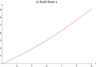
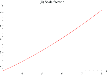
Figure 1: Plots of scale factors versus cosmic time $t$: (i) $a(t)$ versus $t$;
(ii) $b(t)$ versus $t$ for $\zeta_{1}=0.15$, $\zeta_{2}=0.09$, $\zeta_{4}=-0.99$, $\zeta_{5}=0.5$, $\beta_{0}=0.1$.

Both plots of Figure 1 represent graphical analysis of the scale factors $a$ and $b$ which show the increasing behavior of both scale factors in $x$ and $y,~{}z$-directions, respectively. This increasing nature of scale factors indicates the cosmic accelerated expansion in all directions. The graphical analysis of Hubble and deceleration parameters is shown in Figure 2. Figure 2(i) shows that the Hubble parameter grows continuously representing expanding universe whereas Figure 2(ii) shows negative deceleration parameter which corresponds to accelerated expansion of the universe. In Figure 3, the first plot indicates that the effective EoS parameter corresponds to quintessence phase while Figure 3(ii) represents correspondence of the constructed model with standard $\Lambda$CDM universe model. Thus, the analysis of cosmological parameters implies that the universe experiences accelerated expansion for BI universe model in the context of $f(R,T)$ gravity.

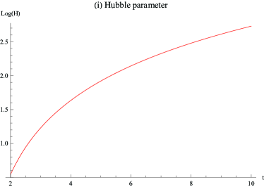
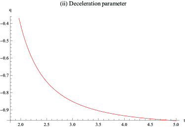
Figure 2: Plots of (i) Hubble parameter and (ii) deceleration parameter versus cosmic time $t$ for $\zeta_{6}=-0.99$.

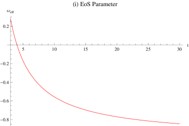
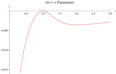
Figure 3: Plots of (i) EoS Parameter and (ii) r-s parameters versus cosmic time $t$ for $\zeta_{6}=-0.99$.

Case II: $\alpha_{2}=\frac{1}{2}$

For $\alpha_{2}=\frac{1}{2}$, the solutions become

$$\alpha=-\frac{5}{2}\beta_{0}ab^{\frac{1}{2}},\quad\beta=\beta_{0}b^{\frac{3}{2}},$$

whereas Eq.(27) yields

$$\delta = 0,\quad h(T)=-2\Lambda+c_{1}T,\quad p=c_{2}a^{\frac{3c_{1}^{2}-3c_{1}-1}{3c_{1}-1}}b^{\frac{3(5c_{1}^{2}-4c_{1}-2)}{2(3c_{1}-1)}},$$

$$\rho = \left(\frac{3c_{1}-1}{c_{1}-2}\right)c_{2}a^{\frac{3c_{1}^{2}-3c_{1}-1}{3c_{1}-1}}b^{\frac{3(5c_{1}^{2}-4c_{1}-2)}{2(3c_{1}-1)}}.$$

The above solutions satisfy the system of Eqs.(17)-(25) for $c_{1}=\frac{3\pm\sqrt{21}}{6}$. Under this condition, the solutions and considered model of $f(R,T)$ gravity take the following form

$$\alpha = -\frac{5}{2}\beta_{0}ab^{\frac{1}{2}},\quad\beta=\beta_{0}b^{\frac{3}{2}},\quad\gamma,\delta=0,\quad h(T)=-2\Lambda+\left(\frac{3\pm\sqrt{21}}{6}\right)T,$$

$$p = c_{2}b^{\frac{1}{2}},\quad\rho=\left(\frac{-3\mp\sqrt{21}}{9\mp\sqrt{21}}\right)c_{2}b^{\frac{1}{2}},\quad f(R,T)=R+\left(\frac{3\pm\sqrt{21}}{6}\right)T,$$

where $T=\left(\frac{30\mp 2\sqrt{21}}{9\mp\sqrt{21}}\right)c_{2}b^{\frac{1}{2}}$. Here, the constructed model ignores Dolgov-Kawasaki instability as $f_{R},~{}f_{RR},~{}1+f_{T}>0$. The symmetry generator and its corresponding conserved quantity turn out to be

$$K=-\frac{5}{2}\beta_{0}ab^{\frac{1}{2}}\frac{\partial}{\partial a}+\beta_{0}b^{\frac{3}{2}}\frac{\partial}{\partial b},\quad\Sigma=\beta_{0}[6ab^{\frac{3}{2}}\dot{b}-4\dot{a}b^{\frac{5}{2}}].$$

We consider $z$ to be a cyclic variable which yields

$$v=\chi_{0}a^{\frac{2}{5}}b,\quad z=-\frac{2b^{-\frac{1}{2}}}{\beta_{0}},$$

where $\chi_{0}$ denotes arbitrary constant. The corresponding inverse point transformation leads to

$$a = \chi_{1}v^{\frac{5}{2}}\left(-\frac{\beta_{0}z}{2}\right)^{5},\quad b=\chi_{2}\left(-\frac{\beta_{0}z}{2}\right)^{-2},$$

$$\quad p = c_{2}\chi_{2}\left(-\frac{\beta_{0}z}{2}\right)^{-1}\quad\rho=\left(\frac{-3\mp\sqrt{21}}{9\mp\sqrt{21}}\right)c_{2}\chi_{2}\left(-\frac{\beta_{0}z}{2}\right)^{-1},$$

where $\chi_{1},\chi_{2}$ are arbitrary constants. For these solutions, the Lagrangian (6) becomes

$$\mathcal{L} = -2\beta_{0}\chi_{1}\chi_{2}^{2}\left[5v^{\frac{3}{2}}\dot{v}-6\beta_{0}v^{\frac{5}{2}}\dot{z}^{2}\left(-\frac{\beta_{0}z}{2}\right)^{-1}\right]+c_{2}v^{\frac{5}{2}}\left[4\left(\frac{3\pm\sqrt{21}}{6}\right)\right.$$

$$\times \left.\left(\frac{6\mp\sqrt{21}}{9\mp\sqrt{21}}\right)-1\right],$$

which depends upon the cyclic variable $z$. Thus, the resulting symmetry generator for $\alpha_{2}=0$ yields scaling symmetry providing more significant results as compared to $\alpha_{2}=\frac{1}{2}$.

3.2 $f(R,T)=f_{1}(R)+f_{2}(T)$

Here we consider $f(R,T)$ model which does not encourage any absolute non-minimal coupling of curvature and matter. For vector field $K$ (14), we substitute this model in Eqs.(17)-(23) and (25) yielding the coefficients of symmetry generator in the form

$$\alpha = -\frac{2ac_{3}}{b\sqrt{f^{\prime}_{1}(R)}}-2ac_{4}\ln(f^{\prime}_{1}(R))-\frac{2c_{5}}{\sqrt{b}}-4\ln(b)ac_{4}-6\ln(b)c_{6}a+c_{7}a,$$

$$\beta = \frac{c_{3}}{\sqrt{f^{\prime}_{1}(R)}}+(c_{8}+\ln(f^{\prime}_{1}(R))c_{4})b-(c_{4}+c_{6})b\ln(b)+c_{6}b\ln(a),$$

$$\gamma = -\frac{2}{\sqrt{f^{\prime}_{1}(R)}f^{\prime\prime}_{1}(R)b}\left[b((-3c_{4}-4c_{6})\ln(b)+c_{4}+c_{8}+\frac{c_{7}}{2}\right.$$

$$+ \left.c_{6}+c_{6}\ln(a))(f^{\prime}_{1}(R))^{\frac{3}{2}}-c_{3}f^{\prime}_{1}(R)\right],$$

where prime denotes derivative with respect to $R$ and $c_{i}$ ($i=3,4,5,6,7,8$) are arbitrary constants. Inserting these solutions in Eq.(24), we obtain two solutions for $f_{1}(R)$ as $f_{1}(R)=c_{9}R+c_{10}$ which is similar to the previous case while the second solution increases the complexity of the system. To avoid this situation, we consider $f_{1}(R)=f_{0}R^{n},~{}(n\neq 0,~{}1)$ which yields

$$\alpha = ac_{11},\quad\beta=bc_{12},\quad\gamma=\frac{(c_{11}+2c_{12})R}{1-n},\quad f_{2}(T)=\frac{T}{3}+c_{13},$$

$$p = \frac{1}{12nc_{13}}\left[R^{1-n}b\rho,_{b}-Rc_{13}-6R^{1-n}c_{13}+2R^{1-n}\rho+6nc_{13}R\right],$$

$$\rho = 3f_{0}R^{n}+3c_{13}-\frac{(c_{11}a\rho,_{a}+c_{12}b\rho,_{b})}{(c_{11}+2c_{12})}.$$

These solutions satisfy (17)-(27) for $n=2$ which implies that $f_{1}(R)=f_{0}R^{2}$ and hence this quadratic curvature term describes an indirect non-minimal coupling of the matter components with geometry. Thus the matter contents and model of $f(R,T)$ gravity turn out to be

$$\rho = 3f_{0}R^{2}+3c_{13}+\frac{a^{-1+\frac{c_{12}}{c_{11}}}b}{2},\quad p=\frac{1}{24c_{13}}\left[\frac{3a^{-1+\frac{c_{12}}{c_{11}}}bR^{-1}}{2}+12c_{13}R\right],$$

$$f(R,T) = f_{0}R^{2}+\frac{T}{3}+c_{13},\quad T=3p-\rho.$$

In this case, the constructed $f(R,T)$ model is found to be viable as it preserves stability conditions (31). The corresponding symmetry generator takes the form

$$K=ac_{11}\frac{\partial}{\partial a}+bc_{12}\frac{\partial}{\partial b}-R(c_{11}+2c_{12})\frac{\partial}{\partial R}.$$

This generator yields scaling symmetry with the following conserved factors

$$\Sigma_{1}=4ab^{2}\dot{R}f_{0}-4b^{2}\dot{a}f_{0}R,\quad\Sigma_{2}=-24ab\dot{b}f_{0}R-8ab^{2}\dot{R}f_{0},$$

where $\Sigma_{1}$ and $\Sigma_{2}$ are conserved quantities corresponding to $c_{11}$ and $c_{12}$, respectively.

To reduce the complex nature of the system, we consider $\phi:(a,b,R)\rightarrow(u,v,z)$ implying that $\phi_{K}du=0$, $\phi_{K}dv=0$ and $\phi_{K}dz=1$. In this case, we choose $z$ as cyclic variable which gives

$$u=A_{0}a^{\frac{c_{11}+2c_{12}}{c_{11}}}R,\quad v=A_{1}b^{\frac{c_{11}+2c_{12}}{c_{12}}}R,\quad z=-\frac{1}{c_{11}+2c_{12}}\ln R,$$

where $A_{0}$ and $A_{1}$ denote integration constants. The corresponding inverse point transformation yields

$$a = u^{\frac{c_{11}}{c_{11}+2c_{12}}}e^{c_{11}z},\quad b=v^{\frac{c_{12}}{c_{11}+2c_{12}}}e^{c_{12}z},\quad R=e^{c_{11}+2c_{12}z}.$$

For these solutions, the Lagrangian (6) takes the form

$$\mathcal{L} = \frac{1}{(c_{11}+2c_{12})^{2}}\left(24f_{0}\dot{z}^{2}v^{\frac{2c_{12}}{c_{11}+2c_{12}}}c_{11}^{3}u^{\frac{c_{11}}{c_{11}+2c_{12}}}c_{12}+60f_{0}\dot{z}^{2}v^{\frac{2c_{12}}{c_{11}+2c_{12}}}u^{\frac{c_{11}}{c_{11}+2c_{12}}}\right.$$

$$\times \left.c_{11}^{2}c_{12}^{2}+80f_{0}\dot{z}^{2}v^{\frac{2c_{12}}{c_{11}+2c_{12}}}c_{11}c_{12}^{3}u^{\frac{c_{11}}{c_{11}+2c_{12}}}+16f_{0}\dot{v}\dot{z}u^{\frac{c_{11}}{c_{11}+2c_{12}}}c_{12}^{3}v^{-\frac{c_{11}}{c_{11}+2c_{12}}}\right.$$

$$+ \left.4f_{0}\dot{u}\dot{z}v^{\frac{2c_{12}}{c_{11}+2c_{12}}}c_{11}^{3}u^{-\frac{2c_{12}}{c_{11}+2c_{12}}}-8f_{0}\dot{u}\dot{v}c_{12}c_{11}v^{-\frac{c_{11}}{c_{11}+2c_{12}}}u^{-\frac{2c_{12}}{c_{11}+2c_{12}}}+8f_{0}\dot{u}\dot{z}\right.$$

$$\times \left.v^{\frac{2c_{12}}{c_{11}+2c_{12}}}u^{-\frac{2c_{12}}{c_{11}+2c_{12}}}c_{12}c_{11}^{2}+8f_{0}\dot{v}\dot{z}u^{\frac{c_{11}}{c_{11}+2c_{12}}}v^{-\frac{c_{11}}{c_{11}+2c_{12}}}c_{12}^{2}c_{11}-\left(u^{\frac{c_{11}}{c_{11}+2c_{12}}}e^{c_{11}z}\right)^{\frac{c_{12}}{c_{11}}}\right.$$

$$\times \left.v^{\frac{3c_{12}}{c_{11}+2c_{12}}}e^{3c_{12}z}c_{11}^{2}-4\left(u^{\frac{c_{11}}{c_{11}+2c_{12}}}e^{c_{11}z}\right)^{\frac{c_{12}}{c_{11}}}v^{\frac{3c_{12}}{c_{11}+2c_{12}}}e^{3c_{12}z}c_{12}^{2}-4f_{0}\dot{v}^{2}c_{12}^{2}\right.$$

$$\times \left.u^{\frac{c_{11}}{c_{11}+2c_{12}}}v^{-\frac{2(c_{12}+c_{11})}{c_{11}+2c_{12}}}+48f_{0}\dot{z}^{2}u^{\frac{c_{11}}{c_{11}+2c_{12}}}v^{\frac{2c_{12}}{c_{11}+2c_{12}}}c_{12}^{4}+4v^{\frac{2c_{12}}{c_{11}+2c_{12}}}u^{\frac{c_{11}}{c_{11}+2c_{12}}}\right.$$

$$\times \left.f_{0}c_{11}^{4}\dot{z}^{2}-4\left(u^{\frac{c_{11}}{c_{11}+2c_{12}}}e^{c_{11}z}\right)^{\frac{c_{12}}{c_{11}}}v^{\frac{3c_{12}}{c_{11}+2c_{12}}}e^{3c_{12}z}c_{11}c_{12}\right).$$

Here, the Lagrangian again depends on the cyclic variable $z$. Consequently, this approach does not provide a successive way to evaluate exact solution of the anisotropic universe model in this case.

4 Noether Gauge Symmetry

In this section, we determine Noether gauge symmetry of homogeneous and isotropic as well as anisotropic universe for $f(R,T)=f_{0}R^{n}+h(T)$ model.

4.1 Flat FRW Universe Model

We first consider flat FRW metric given by

$$ds^{2}=-dt^{2}+a^{2}(t)(dx^{2}+dy^{2}+dz^{2}),$$ (37)

where the scale factor $a$ describes expansion in $x,~{}y$ and $z$-directions. For isotropic universe, the Lagrangian depends on configuration space $(a,~{}R,~{}T)$ with tangent space $(a,~{}R,~{}T,~{}\dot{a},~{}\dot{R},~{}\dot{T})$. The metric variation of action (1) with $\mathcal{L}_{m}=p(a)$ leads to

$$\mathcal{L}(a,R,T,\dot{a},\dot{R},\dot{T})=a^{3}[f(R,T)-Rf_{R}(R,T)-Tf_{T}(R,T)+f_{T}(R,T)$$

$$\times(3p(a)-\rho(a))+p(a)]-6(a\dot{a}^{2}f_{R}(R,T)+a^{2}\dot{a}\dot{R}f_{RR}(R,T)$$

$$+a^{2}\dot{a}\dot{T}f_{RT}(R,T)).$$ (38)

For Noether gauge symmetry, the vector field $K$ with its first order prolongation is defined as

$$K = \tau(t,a,R,T)\frac{\partial}{\partial t}+\alpha(t,a,R,T)\frac{\partial}{\partial a}+\beta(t,a,R,T)\frac{\partial}{\partial R}+\gamma(t,a,R,T)\frac{\partial}{\partial T},$$

$$K^{[1]} = \tau\frac{\partial}{\partial t}+\alpha\frac{\partial}{\partial a}+\beta\frac{\partial}{\partial R}+\gamma\frac{\partial}{\partial T}+\dot{\alpha}\frac{\partial}{\partial\dot{a}}+\dot{\beta}\frac{\partial}{\partial\dot{R}}+\dot{\gamma}\frac{\partial}{\partial\dot{T}},$$

where $\tau,~{}\alpha,~{}\beta$ and $\gamma$ are unknown coefficients of vector field to be determined and the time derivatives of these coefficients are

$$\dot{\alpha}=\frac{\partial\alpha}{\partial t}+\dot{a}\frac{\partial\alpha}{\partial a}+\dot{R}\frac{\partial\alpha}{\partial R}+\dot{T}\frac{\partial\alpha}{\partial T}-\dot{a}\left\{\frac{\partial\tau}{\partial t}+\dot{a}\frac{\partial\tau}{\partial a}+\dot{R}\frac{\partial\tau}{\partial R}+\dot{T}\frac{\partial\tau}{\partial T}\right\},$$

$$\dot{\beta}=\frac{\partial\beta}{\partial t}+\dot{a}\frac{\partial\beta}{\partial a}+\dot{R}\frac{\partial\beta}{\partial R}+\dot{T}\frac{\partial\beta}{\partial T}-\dot{R}\left\{\frac{\partial\tau}{\partial t}+\dot{a}\frac{\partial\tau}{\partial a}+\dot{R}\frac{\partial\tau}{\partial R}+\dot{T}\frac{\partial\tau}{\partial T}\right\},$$

$$\dot{\gamma}=\frac{\partial\gamma}{\partial t}+\dot{a}\frac{\partial\gamma}{\partial a}+\dot{R}\frac{\partial\gamma}{\partial R}+\dot{T}\frac{\partial\gamma}{\partial T}-\dot{T}\left\{\frac{\partial\tau}{\partial t}+\dot{a}\frac{\partial\tau}{\partial a}+\dot{R}\frac{\partial\tau}{\partial R}+\dot{T}\frac{\partial\tau}{\partial T}\right\}.$$

The existence of Noether gauge symmetry demands

$$K^{[1]}\mathcal{L}+(D\tau)\mathcal{L}=DG(t,a,R,T),$$ (39)

where $G$ represents gauge function and $D=\partial_{t}+\dot{a}\partial_{a}+\dot{R}\partial_{R}+\dot{T}\partial_{T}$. Substituting the values of vector field, its first order prolongation and corresponding derivatives of coefficients in Eq.(39), we obtain the following system of equations

$$\tau,_{{}_{a}}=0,\quad\tau,_{{}_{R}}=0,\quad\tau,_{{}_{T}}=0,\quad G,_{{}_{T}}=0,$$ (40)

$$n(n-1)f_{0}R^{n-2}a^{2}\alpha,_{{}_{R}}=0,$$ (41)

$$n(n-1)f_{0}a^{2}R^{n-2}\alpha,_{{}_{T}}=0,$$ (42)

$$2a\alpha,_{{}_{T}}+(n-1)aR^{-1}\beta,_{{}_{T}}=0,$$ (43)

$$6n(n-1)f_{0}a^{2}R^{n-2}\alpha,_{{}_{t}}=-G,_{{}_{R}},$$ (44)

$$nf_{0}R^{n-1}[2a\alpha,_{{}_{t}}+(n-1)a^{2}R^{-1}\beta,_{{}_{t}}]=-G,_{{}_{a}},$$ (45)

$$\alpha+(n-1)aR^{-1}\beta+2a\alpha,_{{}_{a}}-a\tau,_{{}_{t}}+(n-1)a^{2}R^{-1}\beta,_{{}_{a}}=0,$$ (46)

$$2(n-1)R^{-1}\alpha+(n-1)(n-2)aR^{-2}\beta+(n-1)aR^{-1}\alpha,_{{}_{a}}+2\alpha,_{{}_{R}}-(n-1)$$

$$\times aR^{-1}\tau,_{{}_{t}}+(n-1)aR^{-1}\beta,_{{}_{R}}=0,$$ (47)

$$\alpha[3a^{2}\{f_{0}R^{n}(1-n)+h(T)-Th(T),_{{}_{T}}+h(T),_{{}_{T}}(3p-\rho)+p\}+a^{3}\{h(T),_{{}_{T}}$$

$$\times(3p,_{{}_{a}}-\rho,_{{}_{a}})+p,_{{}_{a}}\}]-n(n-1)f_{0}a^{3}R^{n-1}\beta+a^{3}\gamma h(T),_{{}_{T}T}(3p-\rho-T)$$

$$+a^{3}\tau,_{{}_{t}}\{f_{0}R^{n}(1-n)+h(T)-Th(T),_{{}_{T}}+h(T),_{{}_{T}}(3p-\rho)+p\}=G,_{{}_{t}}.$$ (48)

Solving the above system, it follows that

$$\tau = \frac{\xi_{4}t(3\xi_{11}\xi_{2}-\xi_{3}\xi_{10})}{\xi_{11}}+\xi_{13},\quad\alpha=\xi_{4}(\xi_{2}a+\xi_{3}a^{-1}),$$

$$\beta = \frac{\xi_{4}\xi_{3}(\xi_{10}+\xi_{11}a^{-2})R}{\xi_{11}(1-n)},\quad G=\frac{\xi_{1}t}{2},\quad\gamma=0,$$

where $\xi_{i}$ are arbitrary constants. For these coefficients, the symmetry generator becomes

$$K = \left(\frac{\xi_{4}t(3\xi_{11}\xi_{2}-\xi_{3}\xi_{10})}{\xi_{11}}+\xi_{13}\right)\frac{\partial}{\partial t}+\left(\frac{\xi_{4}\xi_{3}(\xi_{10}+\xi_{11}a^{-2})R}{\xi_{11}(1-n)}\right)\frac{\partial}{\partial R}$$

$$+ \xi_{4}(\xi_{2}a+\xi_{3}a^{-1})\frac{\partial}{\partial a}.$$

This generator can be split as

$$K_{1} = \frac{\partial}{\partial t},\quad K_{2}=\left(\frac{t(3\xi_{11}\xi_{2}-\xi_{3}\xi_{10})}{\xi_{11}}\right)\frac{\partial}{\partial t}+\left(\frac{\xi_{3}(\xi_{10}+\xi_{11}a^{-2})R}{\xi_{11}(1-n)}\right)\frac{\partial}{\partial R}$$

$$+ (\xi_{2}a+\xi_{3}a^{-1})\frac{\partial}{\partial a},$$

where the first generator corresponds to energy conservation. The corresponding conserved quantities are

$$\Sigma_{1} = -\frac{t(3\xi_{11}\xi_{2}-\xi_{3}\xi_{10})}{\xi_{11}}\left[a^{3}(f_{0}R^{n}(1-n)+\epsilon_{0}-\frac{\rho}{3})-6(a\dot{a}^{2}+(n-1)\right.$$

$$\times \left.a^{2}\dot{a}\dot{R}R^{-1})nf_{0}R^{n-1}\right]+6anf_{0}R^{n-1}(2\dot{a}-(n-1)aR^{-1}\dot{R})\left[(\xi_{2}a+\xi_{3}a^{-1})\right.$$

$$- \left.\frac{t\dot{a}(3\xi_{11}\xi_{2}-\xi_{3}\xi_{10})}{\xi_{11}}\right]-6n(n-1)f_{0}a^{2}R^{n-2}\dot{a}\left[\frac{\xi_{3}(\xi_{10}+\xi_{11}a^{-2})R}{\xi_{11}(1-n)}\right.$$

$$+ \left.\frac{t\dot{R}(3\xi_{11}\xi_{2}-\xi_{3}\xi_{10})}{\xi_{11}}\right],$$

$$\Sigma_{2} = -a^{3}(f_{0}R^{n}(1-n)+\epsilon_{0}-\frac{\rho}{3})-6(a\dot{a}^{2}+2(n-1)a^{2}\dot{a}\dot{R}R^{-1})nf_{0}R^{n-1}.$$

4.2 Bianchi I Universe Model

Here we investigate Noether gauge symmetry for BI universe model. In this case, the vector field and corresponding first order prolongation take the form

$$K = \tau(t,a,b,R,T)\frac{\partial}{\partial t}+\alpha(t,a,b,R,T)\frac{\partial}{\partial a}+\beta(t,a,b,R,T)\frac{\partial}{\partial b}$$

$$+ \gamma(t,a,b,R,T)\frac{\partial}{\partial R}+\delta(t,a,b,R,T)\frac{\partial}{\partial T},$$

$$K^{[1]} = \tau\frac{\partial}{\partial t}+\alpha\frac{\partial}{\partial a}+\beta\frac{\partial}{\partial b}+\gamma\frac{\partial}{\partial R}+\delta\frac{\partial}{\partial T}+\dot{\alpha}\frac{\partial}{\partial\dot{a}}+\dot{\beta}\frac{\partial}{\partial\dot{b}}+\dot{\gamma}\frac{\partial}{\partial\dot{R}}+\dot{\delta}\frac{\partial}{\partial\dot{T}},$$

where

$$\dot{\alpha}=D\alpha-\dot{a}D\tau,\quad\dot{\beta}=D\beta-\dot{b}D\tau,\quad\dot{\gamma}=D\gamma-\dot{R}D\tau,\quad\dot{\delta}=D\delta-\dot{T}D\tau.$$

Using the above vector field, its prolongation and coefficients derivatives in the condition of the existence of Noether gauge symmetry, we formulate the following system of nonlinear partial differential equations as

$$\tau,_{{}_{a}}=0,\quad\tau,_{{}_{b}}=0,\quad\tau,_{{}_{R}}=0,\quad\tau,_{{}_{T}}=0,\quad G,_{{}_{T}}=0,$$ (62)

$$b\alpha,_{{}_{R}}+2a\beta,_{{}_{R}}=0,$$

$$b\alpha,_{{}_{T}}+2a\beta,_{{}_{T}}=0,$$

$$2\beta,_{{}_{a}}+(n-1)bR^{-1}\gamma,_{{}_{a}}=0,$$

$$2\beta,_{{}_{T}}+(n-1)bR^{-1}\gamma,_{{}_{T}}=0,$$

$$b\alpha,_{{}_{T}}+a\beta,_{{}_{T}}+(n-1)abR^{-1}\gamma,_{{}_{T}}=0,$$

$$n(n-1)f_{0}R^{n-2}[2b^{2}\alpha,_{{}_{t}}+4ab\beta,_{{}_{t}}]=-G,_{{}_{R}},$$

$$nf_{0}R^{n-1}[4b\beta,_{{}_{t}}+2(n-1)b^{2}R^{-1}\gamma,_{{}_{t}}]=-G,_{{}_{a}},$$

$$nf_{0}R^{n-1}[4b\alpha,_{{}_{t}}+4a\beta,_{{}_{t}}+4(n-1)abR^{-1}\gamma,_{{}_{t}}]=-G,_{{}_{b}},$$

$$\alpha+(n-1)aR^{-1}\gamma+2b\alpha,_{{}_{b}}+2a\beta,_{{}_{b}}+2(n-1)abR^{-1}\gamma,_{{}_{b}}+a\tau,_{{}_{t}}=0,$$

$$2\beta+2(n-1)bR^{-1}\gamma+2b\alpha,_{{}_{a}}+2a\beta,_{{}_{a}}+2b\beta,_{{}_{b}}+2(n-1)abR^{-1}\gamma,_{{}_{a}}$$

$$+(n-1)b^{2}R^{-1}\gamma,_{{}_{b}}-2b\tau,_{{}_{t}}=0,$$

$$2(n-1)R^{-1}\beta+(n-1)(n-2)bR^{-2}\gamma+(n-1)bR^{-1}\alpha,_{{}_{a}}+2\beta,_{{}_{R}}$$

$$+2(n-1)aR^{-1}\beta,_{{}_{a}}+(n-1)bR^{-1}\gamma,_{{}_{R}}-(n-1)bR^{-1}\tau,_{{}_{t}}=0,$$

$$2(n-1)bR^{-1}\alpha+2(n-1)aR^{-1}\beta+2(n-1)(n-2)abR^{-2}\gamma+2b\alpha,_{{}_{R}}$$

$$+(n-1)b^{2}R^{-1}\alpha,_{{}_{b}}+2(n-1)abR^{-1}\beta,_{{}_{b}}+2a\beta,_{{}_{R}}+2(n-1)abR^{-1}\gamma,_{{}_{R}}$$

$$-2(n-1)abR^{-1}\tau,_{{}_{t}}=0,$$

$$b^{2}\alpha[f_{0}R^{n}(1-n)+h(T)-Th(T),_{{}_{T}}+h(T),_{{}_{T}}(3p-\rho)+p+a\{h(T),_{{}_{T}}$$

$$\times(3p,_{{}_{a}}-\rho,_{{}_{a}})+p,_{{}_{a}}\}]+\beta[2ab(f_{0}R^{n}(1-n)+h(T)-Th(T),_{{}_{T}}+h(T),_{{}_{T}}$$

$$\times(3p-\rho)+p)+ab^{2}\{h(T),_{{}_{T}}(3p,_{{}_{b}}-\rho,_{{}_{b}})+p,_{{}_{b}}\}]-n(n-1)f_{0}ab^{2}R^{n-1}\gamma$$

$$+ab^{2}\delta h(T),_{{}_{T}T}(3p-\rho-T)+ab^{2}\tau,_{{}_{t}}\{f_{0}R^{n}(1-n)+h(T)-Th(T),_{{}_{T}}$$

$$+h(T),_{{}_{T}}(3p-\rho)+p\}=G,_{{}_{t}}.$$

We solve this system of equations

$$\tau = \eta_{1},\quad G=(\eta_{2}t+\eta_{3})\eta_{4}\eta_{5},\quad\alpha=\eta_{5}\eta_{6}a,\quad\beta=\eta_{5}\eta_{6}b,$$

$$\gamma = \frac{\eta_{5}\eta_{6}R}{2(1-n)},\quad\delta=0,\quad\rho=-\frac{3\eta_{2}\eta_{4}(\eta_{7}+\eta_{8}\ln a)}{ab^{2}\eta_{6}\eta_{8}},$$

$$p = -\frac{1}{2nf_{0}}[f_{0}R^{n}+R^{1-n}\eta_{9}-Rnf_{0}],$$

$$f(R,T) = f_{0}R^{n}-\frac{1}{6nf_{0}}[f_{0}R^{n}+R^{1-n}\eta_{9}-Rnf_{0}]-\frac{\eta_{2}\eta_{4}(\eta_{7}+\eta_{8}\ln a)}{ab^{2}\eta_{6}\eta_{8}},$$

where the constants $\eta_{i}$ are redefined. The solution of these coefficients lead to

$$K = \eta_{1}\frac{\partial}{\partial t}+\eta_{5}\eta_{6}a\frac{\partial}{\partial a}+\eta_{5}\eta_{6}b\frac{\partial}{\partial b}+\frac{\eta_{5}\eta_{6}R}{2(1-n)}\frac{\partial}{\partial R}.$$

This generator can be split as

$$K_{1}=\frac{\partial}{\partial t},\quad K_{2}=a\frac{\partial}{\partial a}+b\frac{\partial}{\partial b}+\frac{R}{2(1-n)}\frac{\partial}{\partial R},$$

where the first generator yields energy conservation whereas the second generator provides scaling symmetry. The corresponding conserved quantities are

$$\Sigma_{1} = -ab^{2}[(f_{0}R^{n}(1-n)+\epsilon_{1}-\frac{\rho}{3})-nf_{0}R^{n-1}(2a\dot{b}^{2}+(n-1)R^{-1}(2b^{2}\dot{a}\dot{R}$$

$$+ 4ab\dot{b}\dot{R})+4b\dot{a}\dot{b})],$$

$$\Sigma_{2} = \eta_{2}t+\eta_{3}-4b^{2}\dot{a}nf_{0}R^{n-1}.$$

5 Final Remarks

In this paper, we have discussed Noether and Noether gauge symmetries of BI universe model in $f(R,T)$ gravity. We have formulated Noether symmetry generators, corresponding conserved quantities, matter contents ($p,~{}\rho$) as well as explicit forms of generic function $f(R,T)$ for BI model via two theoretical models of $f(R,T)$ gravity, i.e., $R+2\Lambda+h(T)$ and $f_{0}R^{n}+h(T)$. We have also evaluated Noether gauge symmetries and conserved quantities of homogeneous isotropic as well as anisotropic universe models for $f_{0}R^{n}+h(T)$ model.

For BI universe model, we have found two Noether symmetry generators for the first model in which the first generator gives scaling symmetry. We have solved the system by introducing cyclic variable which lead to exact solution of the scale factors and $f(R,T)$ model. The graphical behavior of scale factors indicate that the universe undergoes an expansion in $x,~{}y$ and $z$-directions. To evaluate exact solution of the anisotropic universe model for the second symmetry generator, we have constructed Lagrangian in terms of cyclic variable. The Lagrangian violates the mapping $\phi_{K}dz=1$ as it is not independent of cyclic variable $z$. Thus, the symmetry generator with scaling symmetry yields exact solution of the anisotropic universe model. We have investigated graphical behavior of the cosmological parameters, i.e., Hubble and deceleration parameters for this solution. This indicates an accelerated expansion of the universe while EoS parameter corresponds to quintessence phase. The trajectory of $r$ and $s$ parameters indicates that the constructed $f(R,T)$ model corresponds to standard $\Lambda$CDM model. For the second model ($f(R,T)=f_{1}(R)+f_{2}(T)$) when $f_{1}(R)=f_{0}R^{n}$, the symmetry generator provides scaling symmetry for $n=2$. This implies that the scaling symmetry induces an indirect non-minimal quadratic curvature matter coupling in this gravity.

Finally, we have discussed Noether gauge symmetry and associated conserved quantities of flat FRW and BI universe models. The time coefficient of symmetry generator is found to be $t$ dependent for FRW universe but becomes constant for BI model while gauge function is non-zero in both cases. The symmetry generator provides energy conservation for isotropic universe whereas for anisotropic universe, we have energy conservation along with scaling symmetry. In the previous work [28], we have formulated exact solution through Noether symmetry approach for LRS BI universe using $f(R)$ power-law model. The cosmological parameters correspond to accelerated expanding universe while the EoS parameter describes phantom divide line from quintessence to phantom phase. The Noether symmetry generator provides scaling symmetry whereas Noether gauge symmetry yields energy conservation with constant time coefficient of symmetry generator and gauge term. Here, we have discussed exact solution via Noether symmetry for BI model. The cosmological parameters yield consistent results but EoS parameter corresponds to phantom era. In case of Noether gauge symmetry, we have found time dependent gauge term and time coefficient of symmetry generator for flat FRW model but this time coefficient remains constant for BI model. Thus, the Noether and Noether gauge symmetries yield more symmetries for non-minimal curvature matter coupling in $f(R,T)$ gravity as compared to $f(R)$ gravity.

Acknowledgment

This work has been supported by the Pakistan Academy of Sciences Project.

References

- [1] Felice, A.D. and Tsujikawa, S.: Living Rev. Rel. 13(2010)3; Nojiri, S. and Odintsov, S.D.: Phys. Rept. 505(2011)59; Bamba, K., Capozziello, S., Nojiri, S. and Odintsov, S.D.: Astrophys. Space Sci. 342(2012)155.
- [2] Starobinsky, A.A.: J. Exp. Theor. Phys. Lett. 86(2007)157.
- [3] Nojiri, S. and Odintsov, S.D.: Phys. Lett. B 599(2004)137.
- [4] Harko,T., Lobo, F.S.N., Nojiri, S. and Odintsov, S.D.: Phys. Rev. D 84(2011)024020.
- [5] Sharif, M. and Zubair, M.: J. Cosmol. Astropart. Phys. 03(2012)028; J. Exp. Theor. Phys. 117(2013)248 J. Phys. Soc. Jpn. 82(2013)064001; ibid. 82(2013)014002; Astrophys. Space Sci. 349(2014)52; Gen. Relativ. Gravit. 46(2014)1723.
- [6] Ellis, G.F.R., Maartens, R. and MacCallum, M.A.H.: Relativistic Cosmology (Cambridge University Press, 2012).
- [7] Barrow, J.D. and Turner, M.S.: Nature 292(1982)35; Demianski, M.: Nature 307(1984)140.
- [8] Akarsu, Ö. and Kilinc, C.B.: Astrophys. Space Sci. 326(2010)315.
- [9] Sharif, M. and Zubair, M.: Astrophys. Space Sci. 349(2014)457.
- [10] Shamir, M.F.: Eur. Phys. J. C 75(2015)8.
- [11] Kanakavalli, T. and Ananda, R.G.: Astrophys. Space Sci. 361(2016)206.
- [12] Sharif, M. and Waheed, S.: Can. J. Phys. 88(2010)833.
- [13] Sharif, M. and Waheed, S.: Phys. Scr. 83(2011)015014.
- [14] Sharif, M. and Waheed, S.: J. Cosmol. Astropart. Phys. 02(2013)043.
- [15] Kucukakca, Y., Camci, U. and Semiz, İ.: Gen. Relativ. Gravit. 44(2012)1893.
- [16] Jamil, M., Momeni, D. and Myrzakulov, R.: Eur. Phys. J. C 72(2012)2137.
- [17] Kucukakca, Y.: Eur. Phys. J. C 73(2013)2327.
- [18] Sharif, M. and Shafique, I.: Phys. Rev. D 90(2014)084033.
- [19] Sharif, M. and Fatima, I.: J. Exp. Theor. Phys. 122(2016)104.
- [20] Capozziello, S., Stabile, A. and Troisi, A.: Class. Quantum Grav. 24(2007)2153.
- [21] Vakili, B.: Phys. Lett. B 16(2008)664.
- [22] Jamil, M., Mahomed, F.M. and Momeni, D.: Phys. Lett. B 702(2011)315.
- [23] Hussain, I., Jamil, M. and Mahomed, F.M.: Astrophys. Space Sci. 337(2012)373.
- [24] Shamir, M.F., Jhangeer, A. and Bhatti, A.A.: Chin. Phys. Lett. A 29(2012)080402.
- [25] Kucukakca, Y. and Camci, U.: Astrophys. Space Sci. 338(2012)211.
- [26] Momeni, D., Myrzakulov, R. and G dekli, E.: Int. J. Geom. Methods Mod. Phys. 12(2015)1550101.
- [27] Haghani, Z., Harko, T., Lobo, F.S.N., Sepangi, H.R. and Shahidi, S.: Phys. Rev. D 88(2013)044023; Odintsov, S.D. and Saez-Gomez, D.: Phys. Lett. B 725(2013)437.
- [28] Sharif, M. and Nawazish, I.: J. Exp. Theor. Phys. 120(2014)49.