DESY-16-178

A local factorization of the fermion determinant
in lattice QCD

Marco Cè Scuola Normale Superiore, Piazza dei Cavalieri 7, I-56126 Pisa, Italy

and INFN, Sezione di Pisa, Largo B. Pontecorvo 3, I-56127 Pisa, Italy

E-mail: marco.ce@sns.it

Leonardo Giusti Dipartimento di Fisica, Università di Milano–Bicocca,

and INFN, Sezione di Milano–Bicocca,

Piazza della Scienza 3, I-20126 Milano, Italy

E-mail: Leonardo.Giusti@mib.infn.it

Stefan Schaefer John von Neumann Institute for Computing (NIC),

DESY, Platanenallee 6, D-15738 Zeuthen, Germany

E-mail: Stefan.Schaefer@desy.de

Abstract

We introduce a factorization of the fermion determinant in lattice QCD with Wilson-type fermions that leads to a bosonic action which is local in the block fields. The interaction among gauge fields on distant blocks is mediated by multiboson fields located on the boundaries of the blocks. The resultant multiboson domain-decomposed hybrid Monte Carlo passes extensive numerical tests carried out by measuring standard gluonic observables. The combination of the determinant factorization and of the one of the propagator, that we put forward recently, paves the way for multilevel Monte Carlo integration in the presence of fermions. We test this possibility by computing the disconnected correlator of two flavor-diagonal pseudoscalar densities, and we observe a significant increase of the signal-to-noise ratio due to a two-level integration.

1 Introduction

State of the art algorithms for lattice QCD simulations require first integrating out analytically the Grassmann quark fields, e.g. for two degenerate flavors, working with the partition function

$$Z=\int[dU]\,\{\det D\}^{2}\,e^{-S_{\mathrm{G}}[U]}$$ (1.1)

with $D$ the massive Dirac operator and $S_{\mathrm{G}}$ the gauge action, and then simulating this effective gauge theory by Monte Carlo techniques. As a result, the locality of the original action and of the observables is not manifest anymore, because the fermion determinant and the propagator are nonlocal functionals of the link variables $U$.

While necessary for making lattice QCD simulations feasible, the nonlocality leads to severe limitations in practice. Local (link) update algorithms, the method of choice for pure gauge theory, are not competitive anymore. The effective gauge theory is instead simulated with variants of the global hybrid Monte Carlo (HMC) algorithm [1], with only its local variant performing comparably to other link update techniques [5]. For the same reason, noise reduction techniques based on the locality of the theory, such as multihit or multilevel algorithms [6, 7, 8, 9, 10, 11], have not yet been formulated successfully in theories with fermions. They are expected to lead to an impressive acceleration in those cases where the signal-to-noise ratio decreases exponentially with the distance between the sources [12, 13].

Over the last two decades, there have been many attempts to rewrite the fermion determinant via a local bosonic field theory. In the multiboson (MB) approach [14], the bosonic action is ultralocal. The backreaction from the large number of bosonic fields which are typically required, however, results in stiff gauge links and thus in long autocorrelation times [15]. In the domain-decomposed hybrid Monte Carlo (DD-HMC), the determinants of the block Dirac operators are factorized. The remainder, however, is not small, depends on the gauge field values over the entire lattice, and needs to be represented by boson fields with a nonlocal action [16].

The aim of this paper is to introduce a factorization of the fermion determinant in lattice QCD with Wilson-type fermions which can be represented by a bosonic theory with a local action in the block gauge and pseudofermion fields. The first step consists in factorizing out from the determinant the contribution depending on gauge fields in distant blocks; see Eq. (2.7). In the second step this factor, which deviates from the identity by terms suppressed as $\exp{-M_{\pi}\Delta}$ where $M_{\pi}$ is the pion mass and $\Delta$ is the distance between the blocks, is taken exactly into account by introducing multiboson fields on the boundaries of the blocks involved. As a result the final bosonic action is local in the block fields.

Together with the factorization of the fermion observables presented in Ref. [17], this opens the way for multilevel simulations of QCD. We implement these ideas in a multiboson domain-decomposed hybrid Monte Carlo (MB-DD-HMC), which we test extensively by measuring the two-point correlators of the gluonic energy density, of the topological charge density, and of two flavor-diagonal pseudoscalar densities. In all cases we observe a significant increase of the signal-to-noise ratio due to a two-level integration.

Figure 1: Decomposition of the lattice in three thick time slices.

2 Block decomposition of the determinant

The goal of the derivation in this and in the following section is a decomposition of the effective fermion action in terms which are local in the block gauge and scalar fields. The essential idea can be presented by considering a decomposition of the lattice in three blocks $\Lambda_{i}$, $i=0,1,2$, where each block may be the union of disconnected regions, and the only requirement is that the Dirac operator does not connect the blocks $\Lambda_{0}$ with $\Lambda_{2}$ directly. Without loss of generality, we consider the simple case of a lattice with open boundary conditions in the time direction and specify the blocks to be three thick time slices; see Fig. 1. With minor modifications, the same setup applies also to periodic boundary conditions. The general case, in which more than three regions are considered, is given in Appendix C. With this domain decomposition, the Hermitian $O(a)$-improved massive Wilson-Dirac operator $Q=\gamma_{5}D$ (see Appendix A) takes the block form

$$Q=\left(\begin{matrix}Q_{\Lambda_{0,0}}&Q_{\Lambda_{0,1}}&0\\ Q_{\Lambda_{1,0}}&Q_{\Lambda_{1,1}}&Q_{\Lambda_{1,2}}\\ 0&Q_{\Lambda_{2,1}}&Q_{\Lambda_{2,2}}\\ \end{matrix}\right)\;.$$ (2.2)

It is useful to define projection operators to the subspaces of quark fields supported on the domains $\Lambda_{i}$ as

$$[P_{\Lambda_{i}}\psi](x)=\begin{cases}\psi(x)&x\in\Lambda_{i}\,,\\[10.66977pt] 0&{\rm elsewhere}\;.\end{cases}$$ (2.3)

In the following $P_{\Lambda_{i}}$ indicates the projector irrespectively of the dimension of the full space on which it acts. Following Ref. [17], we define the two-block operators

$$Q_{\Omega^{*}_{i}}=\left(\begin{matrix}Q_{\Lambda_{i,i}}&Q_{\Lambda_{i,i+1}}\\ Q_{\Lambda_{i+1,i}}&Q_{\Lambda_{i+1,i+1}}\end{matrix}\right)\;,$$ (2.4)

where $\Omega^{*}_{i}=\Lambda_{i}\cup\Lambda_{i+1}$ and $i=0,1$. The factorization of the determinant of $Q$ is achieved as described in the following four steps.

Step 1

Introduce the two-block partitioning of the lattice as defined in Appendix B with $\Gamma=\Lambda_{0}\cup\Lambda_{2}$ and $\Gamma^{*}=\Lambda_{1}$. Using Eq. (B.45) the determinant can be factorized as

$$\begin{split}\det\,Q&=\det Q_{\Lambda_{1,1}}\det\,\left(\begin{matrix}Q_{\Lambda_{0,0}}-Q_{\Lambda_{0,1}}Q_{\Lambda_{1,1}}^{-1}Q_{\Lambda_{1,0}}&-Q_{\Lambda_{0,1}}Q_{\Lambda_{1,1}}^{-1}Q_{\Lambda_{1,2}}\\[7.11317pt] -Q_{\Lambda_{2,1}}Q_{\Lambda_{1,1}}^{-1}Q_{\Lambda_{1,0}}&Q_{\Lambda_{2,2}}-Q_{\Lambda_{2,1}}Q_{\Lambda_{1,1}}^{-1}Q_{\Lambda_{1,2}}\end{matrix}\right)\,,\end{split}$$ (2.5)

where the second matrix on the rhs is the Schur complement associated to $\Gamma$.

Step 2

Use again Eq. (B.45) to obtain

$$\det\,Q=\frac{1}{\det\,Q^{-1}_{\Lambda_{1,1}}\det\left[P_{\Lambda_{2}}\,Q^{-1}_{\Omega^{*}_{1}}\,P_{\Lambda_{2}}\right]\det\left[P_{\Lambda_{0}}\,Q^{-1}\,P_{\Lambda_{0}}\right]}\,,$$ (2.6)

where each determinant is the one of the nonzero submatrix indicated; e.g. $\det[P_{\Lambda_{2}}\,Q^{-1}_{\Omega^{*}_{1}}\,P_{\Lambda_{2}}]$ stands for the determinant of the inverse of the Schur complement of $Q^{-1}_{\Omega^{*}_{1}}$ in $\Lambda_{2}$ [see Eq. (B.44)]. For the first two determinants in the denominator, the goal has been reached: they depend only on links from one or two time slices, respectively.

Step 3

Combine Eqs. (2.5), (2.6) and (B.46) to rewrite the last determinant as

$$\frac{1}{\det\left[P_{\Lambda_{0}}\,Q^{-1}\,P_{\Lambda_{0}}\right]}=\frac{1}{\det\left[P_{\Lambda_{0}}\,Q^{-1}_{\Omega^{*}_{0}}\,P_{\Lambda_{0}}\right]}\det\,\left(\begin{matrix}1&P_{\Lambda_{0}}Q^{-1}_{\Omega^{*}_{0}}Q_{\Lambda_{1,2}}\\[7.11317pt] P_{\Lambda_{2}}Q^{-1}_{\Omega^{*}_{1}}Q_{\Lambda_{1,0}}&1\end{matrix}\right)\;.$$ (2.7)

This step is suggested by the fact that for $x,y\in\Lambda_{0}$, the propagator elements $Q^{-1}(x,y)$ are expected to be well approximated by the inverse of $Q_{\Omega^{*}_{0}}$ up to corrections suppressed proportionally to $\exp{-M_{\pi}\Delta}$, where $M_{\pi}$ is the pion mass and $\Delta$ is the thickness of the block $\Lambda_{1}$ [17], see also below.

Step 4

Reduce the last determinant in Eq. (2.7) to the one of a matrix acting on one of the boundaries only. To this end, Eq. (B.45) is employed once more

$$\det\!\!\left(\begin{matrix}1&\!\!\!\!\!\!P_{\Lambda_{0}}\,Q^{-1}_{\Omega^{*}_{0}}Q_{\Lambda_{1,2}}\\[7.11317pt] P_{\Lambda_{2}}\,Q^{-1}_{\Omega^{*}_{1}}Q_{\Lambda_{1,0}}&\!\!\!\!\!\!1\end{matrix}\right)\!\!=\det(1-P_{\partial\Lambda_{0}}Q^{-1}_{\Omega^{*}_{0}}Q_{\Lambda_{1,2}}P_{\partial\Lambda_{2}}Q^{-1}_{\Omega^{*}_{1}}Q_{\Lambda_{1,0}}P_{\partial\Lambda_{0}}),\!\!\!\\$$ (2.8)

where $P_{\partial\Lambda_{0}}$ and $P_{\partial\Lambda_{2}}$ are projectors on the inner boundary of the thick time slices $\Lambda_{0}$ and $\Lambda_{2}$ respectively. They are defined such that

$$P_{\partial\Lambda_{i}}Q_{\Lambda_{i,j}}=Q_{\Lambda_{i,j}}P_{\partial\Lambda_{j}}=Q_{\Lambda_{i,j}}\;,\quad i\neq j\;.$$ (2.9)

In our thick time-slice partitioning the inner boundary of a block is the set of points at a distance $1$ from the previous and the next block.

The factorized formula can finally be written as

$$\det\,Q=\frac{1}{\det\,Q^{-1}_{\Lambda_{1,1}}\det\left[P_{\Lambda_{0}}\,Q^{-1}_{\Omega^{*}_{0}}\,P_{\Lambda_{0}}\right]\det\left[P_{\Lambda_{2}}\,Q^{-1}_{\Omega^{*}_{1}}\,P_{\Lambda_{2}}\right]}\det\,(1-w)\;,$$ (2.10)

where

$$w=P_{\partial\Lambda_{0}}Q^{-1}_{\Omega^{*}_{0}}\,Q_{\Lambda_{1,2}}\,Q^{-1}_{\Omega^{*}_{1}}\,Q_{\Lambda_{1,0}}$$ (2.11)

acts on the inner boundary field $P_{\partial\Lambda_{0}}\psi$.

In Eq. (2.10) $\det Q^{-1}_{11}$ depends on the gauge field in the block $\Lambda_{1}$, $\det\,[P_{\Lambda_{0}}\,Q^{-1}_{\Omega^{*}_{0}}\,P_{\Lambda_{0}}]$ on the gauge fields in $\Lambda_{0}\cup\Lambda_{1}$, and $\det\,[P_{\Lambda_{2}}\,Q^{-1}_{\Omega^{*}_{1}}\,P_{\Lambda_{2}}]$ on the gauge field in $\Lambda_{1}\cup\Lambda_{2}$. Only the (small) correction $\det\,(1-w)$ is a function of all the links of the lattice. Note that $\det(1-w)$ is real since all other determinants entering Eq. (2.10) are real.

Figure 2: Representation of the operator $w$. The black lines are full propagators while the thick dots are insertions of the effective hops; see Eqs. (2.1).

2.1 Magnitude of $w$

To shed some light on the size of the contributions of the global determinant $\det(1-w)$, one can rewrite the matrix in terms of the full propagator $Q^{-1}$. By considering two different partitions of the lattice in two blocks, first $\Lambda_{0}\cup\Lambda_{1}$ and $\Lambda_{2}$, and then $\Lambda_{0}$ and $\Lambda_{1}\cup\Lambda_{2}$, it is easy to show that

$$P_{\partial\Lambda_{0}}Q^{-1}_{\Omega^{*}_{0}}\,Q_{\Lambda_{1,2}} = P_{\partial\Lambda_{0}}Q^{-1}\left\{Q_{\Lambda_{1,2}}+Q_{\Lambda_{2,1}}\,Q^{-1}_{\Omega^{*}_{0}}\,Q_{\Lambda_{1,2}}\right\}\;,$$

$$P_{\partial\Lambda_{2}}Q^{-1}_{\Omega^{*}_{1}}\,Q_{\Lambda_{1,0}} = P_{\partial\Lambda_{2}}Q^{-1}\left\{Q_{\Lambda_{1,0}}+Q_{\Lambda_{0,1}}\,Q^{-1}_{\Omega^{*}_{1}}\,Q_{\Lambda_{1,0}}\right\}\;.$$ (2.12)

Therefore two propagators between the boundaries of the block $\Lambda_{0}$ and $\Lambda_{2}$, each one multiplied by an effective boundary operator, appear in the definition of $w$ (see Fig. 2). Numerical experience shows that, if the thickness $\Delta$ of the block $\Lambda_{1}$ is large enough, each of these propagators will be suppressed proportionally to $\exp{-M_{\pi}\Delta/2}$ [17]. Therefore the norm of $w$ is expected to be suppressed as $\exp{-M_{\pi}\Delta}$.

2.2 Spectrum of $w$

Detailed knowledge of the spectrum of $(1-w)$ is required for the next step. According to Eqs. (2.11) and (B.46), the matrix $w$ can be written as a product of two Hermitian matrices

$$w=[P_{\partial\Lambda_{0}}\,Q^{-1}_{\Omega^{*}_{0}}\,P_{\partial\Lambda_{0}}][Q_{\Lambda_{0,1}}Q_{\Lambda_{1,1}}^{-1}Q_{\Lambda_{1,2}}\,Q^{-1}_{\Omega^{*}_{1}}\,Q_{\Lambda_{2,1}}Q_{\Lambda_{1,1}}^{-1}Q_{\Lambda_{1,0}}]$$ (2.13)

acting on the interior boundary of the block $\Lambda_{0}$, which in turn implies that $w$ is similar to $w^{\dagger}$ [18]. The characteristic polynomial of $w$ has therefore real coefficients, and the complex eigenvalues $\delta_{i}$ come in conjugate pairs. The spectrum of $w$ is symmetric with respect to the real axis, and the determinant of $(1-w)$ is real as anticipated. As a consequence of Sec. 2.1, the modulus of the eigenvalues $\delta_{i}$ are expected to be suppressed proportionally to $\exp{-M_{\pi}\cdot\Delta}$.

3 Multiboson factorization

In the previous section, the goal of factorizing the determinant into contributions which depend on the gauge field in the neighboring thick time slices has almost been reached. Only the determinant of $(1-w)$ in Eq. (2.10) depends on the gauge field over the whole lattice. For a suitably chosen thickness of the central thick time slice, however, all eigenvalues of $w$ are expected to satisfy $|\delta_{i}|\ll 1$. This in turn implies a large spectral gap for the matrix $(1-w)$, a fact which makes it possible to express its determinant through a polynomial approximation of $(1-w)^{-1}$.

3.1 Polynomial approximation

As reviewed in Appendix D, a generalization of Lüscher’s original multiboson proposal [14] to complex matrices [19, 20, 21] starts by approximating the function $1/z$, with $z\in\mathbb{C}$, by the polynomial

$$P_{N}(z)\equiv\frac{1-R_{N+1}(z)}{z}=c_{N}\prod_{k=1}^{N}(z-z_{k})\;,$$ (3.14)

where $N$ is chosen to be even, and the $N$ roots of $P_{N}(z)$ are obtained by requiring that for the remainder polynomial $R_{N+1}$ holds $R_{N+1}(0)=1$. The roots $z_{k}$ can be chosen to lie on an ellipse passing through the origin of the complex plane with center $1$ and foci $1\pm c$ (see Appendix D),

$$u_{k}=1-z_{k}=\cos{\left(\frac{2\pi k}{N+1}\right)}+i\sqrt{1-c^{2}}\sin{\left(\frac{2\pi k}{N+1}\right)}\;,\quad k=1,\dots,N\;.$$ (3.15)

3.2 Approximation of the determinant

This polynomial can be used to approximate the inverse determinant

$$\det(1-w)\,\det\{P_{N}(1-w)\}=\det\{1-R_{N+1}(1-w)\}\;,$$ (3.16)

where, if for all eigenvalues of $w$ holds $|\delta_{i}|<1$, the rhs side converges exponentially to 1 as $N$ is increased. Since $w$ is similar to $w^{\dagger}$, and the $u_{k}$ come in complex conjugate pairs, the approximate determinant can be written in a manifestly positive form,

$$\det\{P_{N}(1-w)\}^{-1}=C\prod_{k=1}^{N/2}{\det}^{-1}\big{\{}(u_{k}-w)^{\dagger}(u_{k}-w)\big{\}}\\ =C\prod_{k=1}^{N/2}{\det}^{-1}(W_{\sqrt{u_{k}}}^{\dagger}\,W_{\sqrt{u_{k}}})$$ (3.17)

with an irrelevant constant $C$ and

$$W_{z}=\begin{pmatrix}z\,P_{\partial\Lambda_{0}}&P_{\partial\Lambda_{0}}Q^{-1}_{\Omega^{*}_{0}}Q_{\Lambda_{1,2}}\\[7.11317pt] P_{\partial\Lambda_{2}}Q^{-1}_{\Omega^{*}_{1}}Q_{\Lambda_{1,0}}&z\,P_{\partial\Lambda_{2}}\end{pmatrix}\;.$$ (3.18)

In the last equality of Eq. (3.17), the reverse substitution of the one in Eq. (2.8) has been performed. For the determination of the approximation, it is advantageous to work with the operator $w$ (acting on $\partial\Lambda_{0}$ only) since the order of the polynomial is reduced by about a factor of $2$ for a given accuracy. The expression (3.17) with $W_{z}$ acting on $\partial\Lambda_{0}$ and $\partial\Lambda_{2}$, however, allows in the next step for a fully factorized domain decomposition of the fermion action.

3.3 Multiboson action

For two flavors of quarks we can finally represent the determinants by scalar fields [22]

$$\begin{split}&\frac{\det Q^{2}}{\det\{1-R_{N+1}(1-w)\}^{2}}=\frac{1}{\det\,[Q_{\Lambda_{1,1}}^{-1}]^{2}\cdot\det\,[P_{\Lambda_{0}}Q^{-1}_{\Omega^{*}_{0}}P_{\Lambda_{0}}]^{2}\cdot\det\,[P_{\Lambda_{2}}Q^{-1}_{\Omega^{*}_{1}}P_{\Lambda_{2}}]^{2}}\times\\[7.11317pt] &\times\det\,\{P_{N}(1-w)\}^{-2}=\,C^{\prime}\int[d\phi_{0}d\phi_{0}^{\dagger}]e^{-|P_{\Lambda_{0}}Q^{-1}_{\Omega^{*}_{0}}\phi_{0}|^{2}}\int[d\phi_{1}d\phi_{1}^{\dagger}]e^{-|Q_{\Lambda_{1,1}}^{-1}\phi_{1}|^{2}}\cdot\\ &\int[d\phi_{2}d\phi_{2}^{\dagger}]e^{-|P_{\Lambda_{2}}Q^{-1}_{\Omega^{*}_{1}}\phi_{2}|^{2}}\cdot\prod_{k=1}^{N}\left\{\int[d\chi_{k}d\chi_{k}^{\dagger}]e^{-|W_{\sqrt{u_{k}}}\chi_{k}|^{2}}\right\}\;,\\ \end{split}$$ (3.19)

where $C^{\prime}$ is another irrelevant numerical constant. Each scalar field $\phi_{i}$ is confined to the corresponding region $\Lambda_{i}$, $i=0,1,2$. The $N$ fields $\chi_{k}$ live on the outer boundaries of region $\Lambda_{1}$. We can decompose them as $\chi_{k}=\eta_{k}+\xi_{k}$, with $\eta_{k}=P_{\partial\Lambda_{0}}\chi_{k}$ and $\xi_{k}=P_{\partial\Lambda_{2}}\chi_{k}$, and split explicitly the contributions from the inner boundaries of regions $\Lambda_{0}$ and $\Lambda_{2}$ as

$$\begin{split}|W_{z}\chi_{k}|^{2}&=|z|^{2}|\eta_{k}|^{2}+|z|^{2}|\xi_{k}|^{2}+|P_{\partial\Lambda_{2}}Q^{-1}_{\Omega^{*}_{1}}Q_{\Lambda_{1,0}}\eta_{k}|^{2}+|P_{\partial\Lambda_{0}}Q^{-1}_{\Omega^{*}_{0}}Q_{\Lambda_{1,2}}\xi_{k}|^{2}\\ &+\big{[}z(\xi_{k},Q_{\Lambda_{2,1}}Q^{-1}_{\Omega^{*}_{0}}\eta_{k})+z^{*}\,(\xi_{k},Q^{-1}_{\Omega^{*}_{1}}Q_{\Lambda_{1,0}}\eta_{k})+\text{c.c.}\big{]}\;,\end{split}$$ (3.20)

The dependence of the bosonic action from the gauge field in block $\Lambda_{0}$ and $\Lambda_{2}$ is thus factorized. Interestingly, the terms in Eq. (3.20) which will contribute to the forces in region $\Lambda_{0}$ always start (or end) on the inner boundary of $\Lambda_{2}$ and vice versa. The matrices in Eq. (3.20) contain one boundary to boundary quark propagator which is suppressed exponentially in $\Delta$, see Eq. (2.1), and so do the corresponding forces.

3.4 Order of the polynomial

The order of the polynomial can be fixed, for the required precision, by employing Eq. (D.52) in Appendix D. This guarantees that

$${\rm max}_{||v||=1}\,||\,[1-(1-w)P_{N}(1-w)\,]\,v||\leq{\rm max}_{i}\,|\delta_{i}|^{N+1}=|\delta|^{N+1}_{\rm max}$$ (3.21)

where $v$ is a generic vector on which $w$ acts. Then Eq. (3.16), when $|\delta|^{N+1}_{\rm max}\ll 1$ and $\Tr R_{N+1}(1-w)\ll 1$, implies

$$\det(1-w)\,\det\{P_{N}(1-w)\}=1-\Tr R_{N+1}(1-w)+\dots\;.$$ (3.22)

At the first order in the expansion, the relative error which one makes on the determinant is therefore

$$|\Tr R_{N+1}(1-w)|\leq\sum_{i}|\delta_{i}|^{N+1}\leq\sum_{i=1}^{N_{\rm ev}}|\delta_{i}|^{N+1}+(6L^{3}-N_{\rm ev})|\delta_{N_{\rm ev}+1}|^{N+1}\,,$$ (3.23)

where in the last inequality the contribution from the $N_{\rm ev}$ eigenvalues with the highest modules, i.e. $|\delta_{i}|$ sorted decreasingly, has been treated separately and $L$ is the spatial length in lattice units. If most of the modes have a modulus significantly smaller than $|\delta|_{\rm max}$ and if $N$ is large, the sum on the rhs of Eq. (3.23) will not generate a large factor; see below. Given the distribution of the eigenvalues of $w$, the circle centered in $1$ with radius $1$ is a natural choice for the polynomial approximating $(1-w)^{-1}$ that we adopt in the following. However one could optimize further the approximation by working with an ellipse, and tuning the value of $c$.

3.5 Reweighting factor

A given correlation function of a string of fields $O$ can finally be written as

$$\langle O\rangle=\frac{\langle O\,{\cal W}_{N}\rangle_{N}}{\langle{\cal W}_{N}\rangle_{N}} = \frac{\langle O_{\rm fact}\,\rangle_{N}}{\langle{\cal W}_{N}\rangle_{N}}+\frac{\langle O\,{\cal W}_{N}-O_{\rm fact}\rangle_{N}}{\langle{\cal W}_{N}\rangle_{N}}\;,$$ (3.24)

where $O_{\rm fact}$ is a rather precise factorized approximation of $O$ (see Ref. [17] for instance) and $\langle\cdot\rangle_{N}$ indicates the expectation value in the theory defined by the multiboson action at finite $N$. Since both the action and the observable are factorized, the expectation value $\langle O_{\rm fact}\,\rangle_{N}$ can be computed with a multilevel algorithm by generating gauge field configurations with the multiboson action at finite $N$. All other quantities in Eq. (3.24) can be computed with a one-level Monte Carlo procedure. For two flavors, the reweighting factor ${\cal W}_{N}$ is

$${\cal W}_{N}=\det\{1-R_{N+1}(1-w)\}^{2}\,.$$ (3.25)

This expression is easily evaluated as

$${\cal W}_{N}=\frac{\int[d\eta][d\eta^{\dagger}]e^{-|(1-R_{N+1})^{-1}\eta|^{2}}}{\int[d\eta][d\eta^{\dagger}]e^{-\eta^{\dagger}\eta}}\;,$$ (3.26)

where the exponent can be computed by a Taylor expansion, and as usual the integral over $\eta$ can be replaced by random samples. For the special case of a circle, the simplification $R_{N+1}(1-w)=w^{N+1}$ applies.

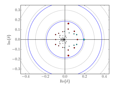
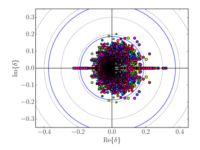
Figure 3: Left: Eigenvalues $\delta_{i}$ of $w$ ($\Delta=12$) with the largest norm for two typical configurations. Right: As in the left panel but for all $200$ configurations. In both panels the blue circles have radius $\bar{\delta}=\exp{-M_{\pi}\Delta}$ and $2\,\bar{\delta}$.

4 Numerical tests on the spectrum of $w$

The feasibility of the whole proposal hinges crucially on the assumption that the spectrum of the operator $(1-w)$ is confined into a disk around $1$ in the complex plane, with a radius significantly below unity. Only in this case, a small number of bosonic fields $N$ in Eq. (3.20) leads to a good enough approximation at reasonable computational cost.

To test this assumption, we have generated a set of $200$ configurations with the Wilson gluonic action and with two flavors of nonperturbatively $O(a)$-improved Wilson quarks as defined in Appendix A, with $\beta=5.3$, $c_{{}_{\rm SW}}=1.90952$, $c_{{}_{\rm F}}=c^{\prime}_{{}_{\rm F}}=1$, $\kappa=0.13625$, $T\times L^{3}=64\times 32^{3}$ and open boundary conditions. The lattice spacing is $0.0652(6)\,\mathrm{fm}$, while the pion mass in lattice units is $M_{\pi}=0.1454(5)$ corresponding to $440(5)$ MeV [23].

For $\Delta=8,12$ and $16$, we have computed with the Arnoldi algorithm the $60$ approximate eigenvalues $\delta_{i}$ of $w$ with the largest absolute value. In the left plot of Fig. 3, they are shown for $\Delta=12$ and on two typical configurations. As expected, the eigenvalues are either real or appear in complex conjugate pairs. For one configuration (green points) the eigenvalue with the largest absolute value is real, while for the other one (red points) two eigenvalues with opposite imaginary parts have the largest absolute value. We find that both possibilities are common; see the last column of Table 1. In the right plot of Fig. 3 we show the eigenvalues $\delta_{i}$ again for $\Delta=12$ but for all configurations. The blue circles in these plots have radius $\bar{\delta}$ and $2\,\bar{\delta}$, where

$$\bar{\delta}=\exp{-M_{\pi}\Delta}\;.$$ (4.27)

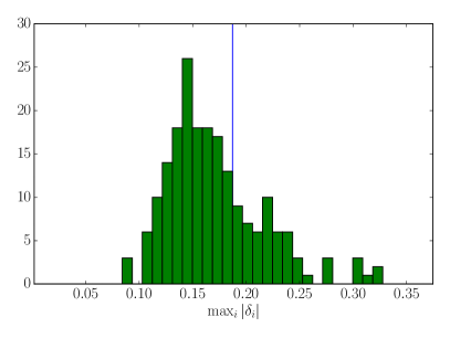
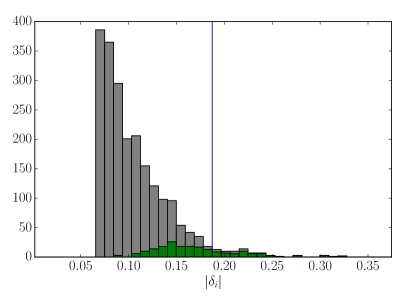
Figure 4: Left: Distribution of the eigenvalue of $w$ ($\Delta=12$) with the largest absolute value. The vertical blue line is at $\absolutevalue{\delta_{i}}=\bar{\delta}$. Right: As in the left panel but for the eigenvalues with $|\delta_{i}|>0.35\,\bar{\delta}$.

Table 1: Properties of the spectrum of $w$ for different values of $\Delta$. $f_{\real}$ is the fraction of configurations for which $\delta_{i}$ with the largest absolute value is real.

$\Delta$	ncfg	$\bar{\delta}$	$\expectationvalue{\max_{i}\absolutevalue{\delta_{i}}}$	$\sigma(\max_{i}\absolutevalue{\delta_{i}})$	$\max\max_{i}\absolutevalue{\delta_{i}}$	$f_{\real}($\mathrm{\char 37\relax}$)$
$8$	$200$	$0.3273$	$0.2886$	$0.0616$	$0.5130$	$48.5$
$12$	$200$	$0.1710$	$0.1692$	$0.0453$	$0.3193$	$46.5$
$16$	$200$	$0.1072$	$0.0951$	$0.0284$	$0.1977$	$45.5$

The distribution of the eigenvalue with the largest magnitude is shown in the left plot of Fig. 4. It is peaked at a value slightly smaller than $\bar{\delta}$, denoted by a vertical blue line, and extends up to $\sim 2\bar{\delta}$. The results for the largest eigenvalue norm computed over the $200$ configurations, its average value and the estimate of its standard deviation are also reported in Table 1. In the right plot of Fig. 4 we also report the distribution of the absolute value of the eigenvalues limited to those with $\absolutevalue{\delta_{i}}>0.35\,\bar{\delta}$.

A clear message emerges from these data. The largest eigenvalue of the relevant operator $w$ decreases proportionally to $\exp{-M_{\pi}\Delta}$, with a prefactor of order $1$. This in turn implies that $(1-w)$ has a large gap if $\Delta$ is properly tuned. The relative error on the determinant computed as in Eq. (3.23) at various values of $N$ compares well with $|\delta|^{N+1}_{\rm max}$ configuration by configuration. No big prefactors appear because the eigenvalues do not accumulate near the maximum one, and the approximation gets exponentially more precise toward the center of the circle. We have also computed the reweighting factor as defined in Eq. (3.26). Its value, again for $N=12$ and estimated with 4 random sources per configuration, deviates from $1$ by at most $4.5\cdot 10^{-6}$ again in line with the expectation. At the level of precision of most contemporary simulations the impact of the reweighting factor is therefore negligible.

5 Numerical implementation of MB-DD-HMC

The effective action in Eq. (3.19) can be simulated using variants of the hybrid Monte Carlo algorithm [1]. The implementation does not pose particular problems. To define the setup for the tests discussed below, we mention a few essential points only. In the following we distinguish between two basic contributions: the determinants of the block operators such as $\det\,[P_{\Lambda_{0}}Q^{-1}_{\Omega^{*}_{0}}P_{\Lambda_{0}}]$, and the multiboson contributions responsible for the coupling between the blocks $\Lambda_{0}$ and $\Lambda_{2}$.

5.1 Block action

In the denominator of Eq. (3.19), there are three determinants derived from the block decomposition of the fermion determinant. For the sake of the presentation we focus on $\det\,[P_{\Lambda_{0}}Q^{-1}_{\Omega^{*}_{0}}P_{\Lambda_{0}}]$, with the other two being treated analogously. Since in general the thick time slices are not particularly thin, further decomposition of this determinant is necessary in order to have a cost-efficient simulation. One possibility is to apply mass preconditioning [24, 25], that is to write

$$\det\,[P_{\Lambda_{0}}Q^{-1}_{\Omega^{*}_{0}}P_{\Lambda_{0}}]=\prod_{i=1}^{N_{\mu}-1}\frac{\det\,[P_{\Lambda_{0}}\{Q_{\Omega^{*}_{0}}(\mu_{i})\}^{-1}P_{\Lambda_{0}}]}{\det\,[P_{\Lambda_{0}}\{Q_{\Omega^{*}_{0}}(\mu_{i+1})\}^{-1}P_{\Lambda_{0}}]}\cdot\det\,[P_{\Lambda_{0}}\{Q_{\Omega^{*}_{0}}(\mu_{N_{\mu}})\}^{-1}P_{\Lambda_{0}}]$$ (5.28)

with $0=\mu_{1}<\mu_{2}<\dots<\mu_{N_{\mu}}$ and $Q_{\Omega^{*}_{0}}(\mu)=Q_{\Omega^{*}_{0}}+i\mu P_{\Lambda_{0}}$. The pseudofermion heatbath is then performed using

$$[P_{\Lambda_{0}}\{Q_{\Omega^{*}_{0}}(\mu)\}^{-1}P_{\Lambda_{0}}]^{-1}=Q_{\Lambda_{0,0}}-Q_{\Lambda_{0,1}}Q_{\Lambda_{1,1}}^{-1}Q_{\Lambda_{1,0}}+i\mu P_{\Lambda_{0}}\,.$$ (5.29)

In the numerical tests described in the following we have used $N_{\mu}=5$, with twisted-mass values $\mu_{i}=0.0,0.001,0.005,0.1,0.5$ for $i=1,\dots,5$.

5.2 Multiboson action

The contribution of the multiboson fields is by construction small and therefore preconditioning does not seem to be necessary in a first implementation. The computation of the forces themselves is straightforward, while the heatbath for the bosonic fields requires further attention.

For the fields $\chi_{k}$, distributed according to the action $S_{\mathrm{b},k}=|W_{\sqrt{u_{k}}}\chi_{k}|^{2}$, the heatbath can be performed in the usual fashion, by acting with the inverse of $W_{\sqrt{u_{k}}}$ on Gaussian random fields located on the inner boundaries of regions $\Lambda_{0}$ and $\Lambda_{2}$. One way to solve the corresponding linear system is discussed in Appendix E. The cost of these inversions is negligible compared to the one of the molecular dynamics evolution. In the numerical tests presented in the following we have used $N=12$ multiboson fields $\chi_{k}$, with the roots $z_{k}$ chosen to lie on the circle of radius $1$ centered in $1$.

6 Numerical tests of MB-DD-HMC

In order to test the potentiality of the two-level MB-DD-HMC algorithm described in the previous section, we have taken a subset of $n_{0}=32$ configurations spaced by at least $80$ molecular dynamics units (MDUs) among the $200$ described in Sec. Section 4, which we can safely assume to be independent. Starting from each of them, we have generated $n_{1}=45$ level-1 configurations spaced by $4$ MDUs by keeping fixed the spatial links on the boundaries $\partial\Lambda_{0}$ and $\partial\Lambda_{2}$ and all the links in between. The region $\Lambda_{1}$ extends between time slices $24$ and $35$, corresponding to a thickness of $\Delta\approx 0.8$ fm and $M_{\pi}\Delta\approx 1.7$.

For the gauge variables in each of the two active regions $\Lambda_{0}$ and $\Lambda_{2}$, the molecular dynamics in the HMC can be integrated with the following nested three-level scheme. The forces derived from the multiboson fields are integrated on the outermost level with a second order Omelyan-Mryglod-Folk (OMF) [26] integrator, with 12 steps per trajectory of length 2. On the second level, all forces derived from the block determinants in Eq. (5.28) are integrated, with one step of the fourth order OMF integrator per outer step. The third level, which consists again of one fourth order OMF step, takes care of the gauge forces. This scheme, which is very similar to the ones used in Ref. [27], leads to an acceptance rate of 94%.

6.1 Correlation functions of gluonic operators

The primary local gluonic observables that we measure to test the algorithm are the energy and the topological charge densities summed over the time slices, i.e.

$$\bar{e}(x_{0})=\frac{1}{4}\sum_{\vec{x}}F_{\mu\nu}^{a}(x)F_{\mu\nu}^{a}(x)\;,\quad\bar{q}(x_{0})=\frac{1}{64\pi^{2}}\,\sum_{\vec{x}}\epsilon_{\mu\nu\rho\sigma}\,F_{\mu\nu}^{a}(x)F_{\rho\sigma}^{a}(x)\;,$$ (6.30)

where the gluon field strength tensor is the one in Eq. (A.41) but with the trace removed. In particular we focus on the expectation value

$$C_{e}(x_{0})=\frac{1}{L^{3}}\langle\bar{e}(x_{0})\rangle\;,$$ (6.31)

and on the correlators

$$C_{ee}(x_{0},y_{0}) = \frac{1}{L^{3}}\langle\bar{e}(x_{0})\,\bar{e}(y_{0})\rangle_{c}\;,$$ (6.32)

$$C_{qq}(x_{0},y_{0}) = \frac{1}{L^{3}}\langle\bar{q}(x_{0})\,\bar{q}(y_{0})\rangle\;.$$ (6.33)

In an analysis of $200$ level-0 configurations each spaced by 8 MDUs, autocorrelations of $\bar{e}(x_{0})$ and $\bar{q}(x_{0})$ are not detectable.

The two-level estimates of the same quantities have been carried out by first averaging, for each of the $n_{0}$ configurations, the densities over the $n_{1}$ level-1 background fields. This gives $n_{0}$ measurements of the improved observables. The figure of merit is the variance of this estimator. In the situation where autocorrelations among the $n_{0}$ level-0 configurations can be neglected, the square root of the variance divided by $\sqrt{n_{0}}$ gives the error of the measurement. Since the cost of the simulation scales linearly in $n_{1}$, the variance itself should decrease with $n_{1}$ to break even.

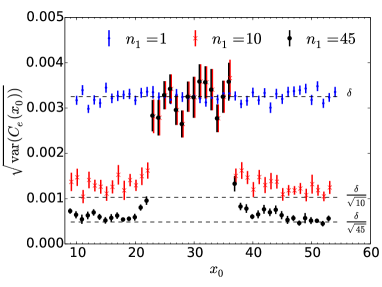
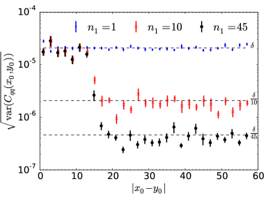
Figure 5: In the left panel, the square root of the variance of the energy density averaged over the time slice $x_{0}$ is shown. In the frozen central region this does not profit from the level-1 updates, while in the active regions, it decreases with the square root of their inverse number. The right plot demonstrates the effectiveness of the multilevel algorithm for the topological charge density correlation function. The time slices $x_{0}$ and $y_{0}=30-x_{0}$ are chosen such that they are symmetric with respect to the frozen region $\Lambda_{1}$. Once $|x_{0}-y_{0}|>12$ they enter the active regions where the square root variance decreases with $1/n_{1}$. In both plots, the horizontal lines indicate the ideal scaling behavior as expected from the variance measured at level 0.

The square root of the variance of $C_{e}(x_{0})$ as a function of $x_{0}$ is shown in the left panel of Fig. 5. In the central region, the links are frozen during the level-1 updates. We therefore do expect the same variance as in the level-0 estimator, but the error of the variance is larger due to the smaller value of $n_{0}$ in this case. Once we move into the active regions $\Lambda_{0}$ and $\Lambda_{2}$, however, the variance of the estimator is clearly improved, in agreement with what is expected from ideal scaling, i.e. $\sqrt{\mathrm{var}(C_{e})}\propto 1/\sqrt{n_{1}}$.

In the right panel the same analysis is shown for the two-point function $C_{qq}$, and analogous results are obtained for $C_{ee}$. Here the full benefit of the method can be realized, because an improved estimator can be constructed by averaging for each of the $n_{0}$ fields the densities in regions $\Lambda_{0}$ and $\Lambda_{2}$ independently before constructing the two-point function. As optimal scaling in this case we expect a reduction of the square root of the variance, and therefore the error, with $1/n_{1}$. The numerical data are in agreement with such a reduction once $x_{0}$ and $y_{0}$ are in two different active regions.

The picture emerging from this analysis is just in line with expectations. In the region where the links are frozen during the level-1 updates no benefit from the multilevel is observed. As soon as the densities are in the active regions $\Lambda_{0}$ and $\Lambda_{2}$, the square root of the variances of the one- and two-point functions are reduced by $1/\sqrt{n_{1}}$ and $1/n_{1}$ respectively. The two-level Monte Carlo works at full potentiality in these regions, with a net gain in the computational cost of the two-point functions of $n_{1}$. This in turn implies that links in the active regions $\Lambda_{0}$ and $\Lambda_{2}$ are regularly updated during the level-1 MB-DD-HMC. In particular no freezing induced by multiboson fields is observed.

6.2 Disconnected pseudoscalar propagator

Quark-line disconnected correlation functions serve as a second test of the method, following our quenched results presented in Ref. [17]. We restrict ourselves to the correlation between two flavor-diagonal pseudoscalar densities,

$$C_{P_{d}}(y_{0},x_{0})=\frac{1}{L^{3}}\,\langle\,\sum_{{\vec{x}}}\tr\{Q^{-1}(x,x)\Big{\}}\times\sum_{{\vec{y}}}\tr\{Q^{-1}(y,y)\Big{\}}\rangle$$ (6.34)

which are decomposed as in Eq. (6.1) of Ref. [17]

$$C_{P_{d}}(y_{0},x_{0})=C^{(\text{f})}_{P_{d}}(y_{0},x_{0})+C^{(\text{r}_{1})}_{P_{d}}(y_{0},x_{0})+C^{(\text{r}_{2})}_{P_{d}}(y_{0},x_{0})\;.$$ (6.35)

In the first contribution, the two propagators in Eq. (6.34) are replaced by approximate propagators with Dirichlet boundary conditions imposed at $x_{0}^{\rm cut}=30$, making this term amenable to multilevel integration. The other two contributions are correction terms which make the equation exact, containing once or twice, respectively, the difference between the full and approximate propagator. Note that in this case there are several options for imposing Dirichlet boundary conditions. They may, for instance, be imposed on the (opposite) respective ends of the frozen region $\Lambda_{1}$.

All the traces appearing on the rhs of Eq. (6.35) are estimated stochastically by inverting the various Dirac operators on the very same $n_{\text{src}}=500$ Gaussian random sources $\eta_{i}$, defined on the whole space-time volume, and by contracting the solution with a time slice of $\eta_{i}$; see Ref. [17] for more details.

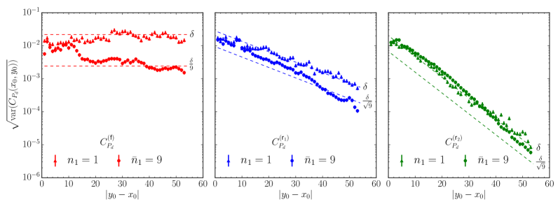
Figure 6: The square root of the variance of the three contributions of the disconnected correlator of two flavor-diagonal pseudoscalar densities [see Eq. (6.35)] are shown as a function of the time separation $|y_{0}-x_{0}|$. The dashed lines indicate the expected asymptotic form, which is constant for the first contributions and falls exponentially $\exp\{-M_{\pi}|y_{0}-x_{0}|/2\}$ and $\exp\{-M_{\pi}|y_{0}-x_{0}|\}$ for the second and third contributions, respectively. In all panels, the lower line indicates the expected reduction from the level-1 updates.

A rough measure of the autocorrelation function of $\sum_{{\vec{x}}}\tr\{Q^{-1}(x,x)\Big{\}}$ from level-0 configurations shows that the autocorrelation time is approximately $\tau_{\mathrm{int}}=10$ MDUs. The $32$ configurations can thus be safely considered as independent when used for level-0 measurements.

As for the gluonic two-point function above, the $C^{(\text{f})}_{P_{d}}(y_{0},x_{0})$ contribution, for $x_{0}<24$ and $y_{0}>35$, is estimated by first averaging, for each of the level-0 configurations, the two traces independently over the $n_{1}$ level-1 background fields. The product of the two means constitutes the improved estimator which is then averaged over the $n_{0}$ measurements. For the other two contributions such an improved estimator is not available. The correlation functions $C^{(\text{r}_{1})}_{P_{d}}$ and $C^{(\text{r}_{2})}_{P_{d}}$ as a whole are first averaged over level 1, giving again $n_{0}$ measurements which are then processed in the usual manner.

While for the first contribution the scaling of the square root variance is expected to be proportional to $n_{1}^{-1}$, for the second and the third it goes at most with $n_{1}^{-1/2}$. Since $n_{1}$ has to be counted in the number of independent measurements and the level-1 updates are spaced by $4$ MDUs only, in the plots we opt for normalizing the number of level-1 updates as $\bar{n}_{1}=n_{1}/(2\,\tau_{\mathrm{int}})=n_{1}/5$. This rescaling has no impact on the correctness of the procedure itself, but relates only to the level of improvement which one can expect from a given number of level-1 updates.

The numerical results for the square root of the variance of $C^{(\text{f})}_{P_{d}}$, $C^{(\text{r}_{1})}_{P_{d}}$, and $C^{(\text{r}_{2})}_{P_{d}}$ are plotted in Fig. 6 as a function of the time separation of the pseudoscalar densities. In all cases $x_{0}$ and $y_{0}$ belong to different domains, $y_{0}>x_{0}$, and they are chosen to be as much as possible equidistant from $x_{0}^{\text{cut}}$. These plots can be directly compared with those on the right column of Fig. 4 in Ref. [17].

Our findings are very similar to the quenched case [17], once one takes into account that in the present computation $12$ slices are frozen instead of $1$. The square root of the variance of $C_{P_{d}}^{(\text{f})}$ (the left plot of Fig. 6) is a flat function of $|y_{0}-x_{0}|$ with sizable deviations near the boundaries of the domains. Up to the largest value that we have, $\bar{n}_{1}=9$, the square root variance decreases approximately as $\bar{n}_{1}^{-1}$ for large $|y_{0}-x_{0}|$; i.e. the two-level Monte Carlo works as expected. For $C_{P_{d}}^{(\text{r}_{1})}$ and $C_{P_{d}}^{(\text{r}_{2})}$, center and right plots in Fig. 6, a strong dependence on $|y_{0}-x_{0}|$ is observed. They are compatible with an exponential behavior of the form $\exp\{-M_{\pi}|y_{0}-x_{0}|/2\}$ and $\exp\{-M_{\pi}|y_{0}-x_{0}|\}$ respectively as suggested by theory.

The picture which emerges is analogous to the one in the quenched case [17]. At large time distances, the statistical error of the standard estimate of the disconnected pseudoscalar propagator is dominated by the one on $C_{P_{d}}^{(\text{f})}$. This is the contribution for which the multilevel is efficient. The second largest contribution is the statistical error on $C_{P_{d}}^{(\text{r}_{1})}$ which, however, is exponentially suppressed as $\exp\{-M_{\pi}|y_{0}-x_{0}|/2\}$. Therefore, once the two-level integration is switched on and a large enough number of $n_{1}$ level-1 configurations is generated, the signal-to-noise ratio increases exponentially in ${|y_{0}-x_{0}|}$ with respect to the standard Monte Carlo.

7 Conclusions

The gauge field dependence of the fermion determinant is factorizable by combining a domain decomposition with a multiboson representation of the (small) interaction among gauge fields on distant blocks. The factorization does not require a particular shape of the three domains, nor does each of them need to be connected.

The resulting action is local in the block scalar and gauge fields and can be simulated by variants of the standard hybrid Monte Carlo algorithm. The measurements of local gluonic observables, such as the energy and the topological charge densities, reveal a good efficiency of the algorithm in updating the gauge field. No particular freezing of the links is observed. The locality of the action can be beneficial for simulations using parallel computers due to reduced communication.

When combined with the recently proposed factorization of the fermion propagator [17], this setup naturally allows for multilevel Monte Carlo integration also in the presence of fermions, opening new perspectives in lattice gauge theories. The numerical test of the disconnected correlator of two flavor-diagonal pseudoscalar densities that we have reported indeed shows that the signal-to-noise ratio increases exponentially with the time distance of the sources when a two-level integration is at work.

Many interesting computations in lattice QCD and other theories are expected to profit from these improvements, especially those which suffer from signal-to-noise ratios which decrease exponentially with the time distance of the sources. Prime examples here are disconnected correlators and/or baryonic two- and three-point functions.

The proposed method relies on two key ingredients: the locality of the Wilson Dirac operator and the (configuration by configuration) exponential decrease of its inverse with the distance between the sink and the source. The ideas and the computational strategy presented here may, therefore, be applicable to very different theories with fermions if they enjoy these very basic properties.

8 Acknowledgments

We thank M. Lüscher for interesting discussions and comments to improve the first version of this paper, in particular regarding the generality of the decomposition proposed here and the simplification of Appendix E. Simulations have been performed on the PC clusters Galileo and Marconi at CINECA (CINECA-INFN and CINECA-Bicocca agreements), PAX at DESY, and Wilson at Milano-Bicocca. We thank these institutions for the computer resources and the technical support. Numerical simulations have been carried out with a modified version of the open-QCD code version 1.4 [28].

Appendix A $O(a)$-improved Wilson-Dirac operator

The massive $O(a)$-improved Wilson-Dirac operator is defined as [29, 30, 27]

$$D=D_{\mathrm{w}}+\delta D_{\mathrm{v}}+\delta D_{\mathrm{b}}+m_{0}\;,$$ (A.36)

where $m_{0}$ is the bare quark mass, $D_{\mathrm{w}}$ is the massless Wilson-Dirac operator

$$D_{\mathrm{w}}=\frac{1}{2}\left\{\gamma_{\mu}(\nabla^{*}_{\mu}+\nabla_{\mu})-\nabla^{*}_{\mu}\nabla_{\mu}\right\}\;,$$ (A.37)

$\gamma_{\mu}$ are the Dirac matrices, and the summation over repeated indices is understood. The covariant forward and backward derivatives $\nabla_{\mu}$ and $\nabla^{*}_{\mu}$ are defined to be

$$\nabla_{\mu}\psi(x)=U_{\mu}(x)\psi(x+\hat{\mu})-\psi(x)\;,\quad\nabla^{*}_{\mu}\psi(x)=\psi(x)-U_{\mu}^{\dagger}(x-\hat{\mu})\psi(x-\hat{\mu})\;,$$ (A.38)

where $U_{\mu}(x)$ are the link fields. The boundary correction terms are defined to be

$$\delta D_{\mathrm{v}}\psi(x) = c_{{}_{\rm SW}}\frac{i}{4}\sigma_{\mu\nu}\widehat{F}_{\mu\nu}(x)\psi(x)\;,$$ (A.39)

$$\delta D_{\mathrm{b}}\psi(x) = \{(c_{{}_{\rm F}}-1)\delta_{x_{0},1}+(c^{\prime}_{{}_{\rm F}}-1)\delta_{x_{0},T-1}\}\,\psi(x)\;,$$ (A.40)

where with open boundary conditions in the time direction $c^{\prime}_{{}_{\rm F}}=c_{{}_{\rm F}}$, $\sigma_{\mu\nu}=\frac{i}{2}[\gamma_{\mu},\gamma_{\nu}]$, and the field strength of the gauge field is

$$\widehat{F}_{\mu\nu}(x)=\frac{1}{8}\{Q_{\mu\nu}(x)-Q_{\nu\mu}(x)\}$$ (A.41)

with

$$Q_{\mu\nu}(x) = U_{\mu}(x)\,U_{\nu}(x+\hat{\mu})\,U^{\dagger}_{\mu}(x+\hat{\nu})\,U^{\dagger}_{\nu}(x)$$

$$+ U_{\nu}(x)\,U^{\dagger}_{\mu}(x-\hat{\mu}+\hat{\nu})\,U^{\dagger}_{\nu}(x-\hat{\mu})\,U_{\mu}(x-\hat{\mu})$$

$$+ U^{\dagger}_{\mu}(x-\hat{\mu})\,U^{\dagger}_{\nu}(x-\hat{\mu}-\hat{\nu})\,U_{\mu}(x-\hat{\mu}-\hat{\nu})\,U_{\nu}(x-\hat{\nu})$$

$$+ U^{\dagger}_{\nu}(x-\hat{\nu})\,U_{\mu}(x-\hat{\nu})\,U_{\nu}(x+\hat{\mu}-\hat{\nu})\,U^{\dagger}_{\mu}(x)\;.$$

We are also interested in the operator $Q=\gamma_{5}D$, which is Hermitian since $D$ satisfies the $\gamma_{5}$-Hermiticity relation $D=\gamma_{5}D^{\dagger}\gamma_{5}$.

Appendix B LU decomposition of a $2\times 2$ block matrix

A $2\times 2$ block matrix can be decomposed as

$$Q=\left(\begin{array}[]{c@{~~}c@{~~}}Q_{\Gamma}\hfil\leavevmode\nobreak\ \leavevmode\nobreak\ &Q_{\partial\Gamma}\hfil\leavevmode\nobreak\ \leavevmode\nobreak\ \\[7.11317pt] Q_{\partial\Gamma^{*}}\hfil\leavevmode\nobreak\ \leavevmode\nobreak\ &Q_{\Gamma^{*}}\hfil\leavevmode\nobreak\ \leavevmode\nobreak\ \end{array}\right)=\left(\begin{array}[]{c@{~~}c@{~~}}I\hfil\leavevmode\nobreak\ \leavevmode\nobreak\ &\;\;Q_{\partial\Gamma}\,Q_{\Gamma^{*}}^{-1}\hfil\leavevmode\nobreak\ \leavevmode\nobreak\ \\[7.11317pt] 0\hfil\leavevmode\nobreak\ \leavevmode\nobreak\ &I\hfil\leavevmode\nobreak\ \leavevmode\nobreak\ \end{array}\right)\left(\begin{array}[]{c@{~~}c@{~~}}S_{\Gamma}\hfil\leavevmode\nobreak\ \leavevmode\nobreak\ &0\hfil\leavevmode\nobreak\ \leavevmode\nobreak\ \\[7.11317pt] Q_{\partial\Gamma^{*}}\hfil\leavevmode\nobreak\ \leavevmode\nobreak\ &Q_{\Gamma^{*}}\hfil\leavevmode\nobreak\ \leavevmode\nobreak\ \end{array}\right)\;,$$ (B.43)

where the Schur complement is defined as

$$S_{\Gamma}=Q_{\Gamma}-Q_{\partial\Gamma}\,Q_{\Gamma^{*}}^{-1}\,Q_{\partial\Gamma^{*}}\;.$$ (B.44)

Its determinant can then be factorized

$$\det\,Q=\det\left(Q_{\Gamma}-Q_{\partial\Gamma}\,Q_{\Gamma^{*}}^{-1}\,Q_{\partial\Gamma^{*}}\right)\,\det Q_{\Gamma^{*}}\;,$$ (B.45)

while the inverse is given by

$$Q^{-1}=\left(\begin{array}[]{c@{~~}c@{~~}}S_{\Gamma}^{-1}\hfil\leavevmode\nobreak\ \leavevmode\nobreak\ &-S^{-1}_{\Gamma}Q_{\partial\Gamma}Q_{\Gamma^{*}}^{-1}\hfil\leavevmode\nobreak\ \leavevmode\nobreak\ \\[7.11317pt] -Q_{\Gamma^{*}}^{-1}Q_{\partial\Gamma^{*}}S^{-1}_{\Gamma}\hfil\leavevmode\nobreak\ \leavevmode\nobreak\ &\;\;Q_{\Gamma^{*}}^{-1}+Q^{-1}_{\Gamma^{*}}Q_{\partial\Gamma^{*}}S^{-1}_{\Gamma}Q_{\partial\Gamma}Q^{-1}_{\Gamma^{*}}\hfil\leavevmode\nobreak\ \leavevmode\nobreak\ \end{array}\right)\;.$$ (B.46)

It is worth noting that $S^{-1}_{\Gamma}$ is the exact inverse of $Q$ if the source and the sink positions are both in $\Gamma$.

Appendix C Even-odd block decomposition of the determinant

The factorization described in Secs. 2 and 3 can be generalized to the case of a lattice decomposed in many thick time slices. The two-block partitioning in step 1 of Sec. 2 generalizes to

$$\Gamma=\bigcup_{\text{even $i$}}\Lambda_{i}\;,\qquad\Gamma^{*}=\bigcup_{\text{odd $i$}}\Lambda_{i}\;,$$ (C.47)

and the operator $Q_{\Omega^{*}_{i}}$ becomes the three-block matrix

$$Q_{\Omega^{*}_{i}}=\begin{pmatrix}Q_{\Lambda_{i-1,i-1}}&Q_{\Lambda_{i-1,i}}&0\\ Q_{\Lambda_{i,i-1}}&Q_{\Lambda_{i,i}}&Q_{\Lambda_{i,i+1}}\\ 0&Q_{\Lambda_{i+1,i}}&Q_{\Lambda_{i+1,i+1}}\end{pmatrix}\qquad i=2,4,\dots$$ (C.48)

with the exception of the first ($i=0$) and the last (if the last block is even) matrices which remain two-block operators. Following the same four-step procedure of Sec. 2, the determinant of the Hermitian Dirac operator is factorized as

$$\det Q=\left(\prod_{\text{odd $i$}}\frac{1}{\det Q^{-1}_{\Lambda_{i,i}}}\right)\left(\prod_{\text{even $i$}}\frac{1}{\det P_{\Lambda_{i}}\,Q^{-1}_{\Omega^{*}_{i}}\,P_{\Lambda_{i}}}\right)\det W_{1}\;,$$ (C.49)

where

$$W_{z}\!\!=\!\!\begin{pmatrix}\ddots&\ddots\\ \ddots&zP_{\partial\Lambda_{i-2}}&\!\!\!\!\!P_{\partial\Lambda_{i-2}}Q_{\Omega^{*}_{i-2}}^{-1}Q_{\Lambda_{i-1,i}}\\[7.11317pt] &\!\!\!\!\!P_{\partial\Lambda_{i}}Q_{\Omega^{*}_{i}}^{-1}Q_{\Lambda_{i-1,i-2}}&zP_{\partial\Lambda_{i}}&\!\!\!\!\!P_{\partial\Lambda_{i}}Q_{\Omega^{*}_{i}}^{-1}Q_{\Lambda_{i+1,i+2}}\\[7.11317pt] &&\!\!\!\!\!P_{\partial\Lambda_{i+2}}Q_{\Omega^{*}_{i+2}}^{-1}Q_{\Lambda_{i+1,i}}&zP_{\partial\Lambda_{i+2}}&\ddots\\[7.11317pt] &&&\ddots&\ddots\end{pmatrix}\,.\!\!\!\!\!$$ (C.50)

The product $W^{\dagger}_{z}W_{z}$ has nonzero matrix elements on the diagonal and among first and second nearest-neighbor even thick time slices. Each term in the corresponding multiboson action, however, depends only on one three-block operator analogously to Eq. (3.20); i.e. the dependence on the gauge field in the interior of the even thick time slices is factorized.

Appendix D Polynomial approximation of $1/z$

The Chebyshev polynomials offer an (asymptotically) optimal polynomial approximation of $1/z$ when $z$ is within an ellipse which does not contain the origin, see Refs. [31, 32] and references therein.

When $z$ is contained in an ellipse centered at a distance $d$ from the origin on the positive real axis, with major and minor radii $a$ and $b$ respectively and with focus distance $c=\sqrt{a^{2}-b^{2}}$, the polynomial approximation of $1/z$ of order $n$ is

$$P_{N}(z)\equiv\frac{1-R_{N+1}(z)}{z}=c_{N}\prod_{k=1}^{N}(z-z_{k})\;,$$ (D.51)

where

$$R_{N+1}(z)\equiv\frac{T_{N+1}\left(\frac{d-z}{c}\right)}{T_{N+1}\left(\frac{d}{c}\right)}\;,$$ (D.52)

with $T_{k}(z)$ being the Chebyshev polynomial of the first kind of degree $k$. The $N$ roots of $P_{N}(z)$ are obtained by requiring that $R_{N+1}(0)=1$, and they are given by

$$z_{k}=d\left(1-\cos{\frac{2\pi k}{N+1}}\right)-i\sqrt{d^{2}-c^{2}}\sin{\frac{2\pi k}{N+1}}\;,\quad k=1,\dots,N\;.$$ (D.53)

They lie on the ellipse in the complex plane with center $d$, foci $d\pm c$, and which passes through zero. By using the definition of the Chebyshev polynomials, a uniform error bound on the approximation is given by

$$|1-zP_{N}(z)|\!=\!|R_{N+1}(z)|\!\leq\!\left(\frac{a+\sqrt{a^{2}-c^{2}}}{d+\sqrt{d^{2}-c^{2}}}\right)^{\!\!N+1}\!\!\!\!\left\{1+\Big{[}\frac{a}{c}+\big{(}\frac{a^{2}}{c^{2}}-1\big{)}^{1/2}\Big{]}^{-2N-2}\right\}\;.$$ (D.54)

D.1 The circle

In the limit $c\rightarrow 0$, when the ellipse becomes a circle centered in $d$ with radius $a=b$, it holds

$$|R_{N+1}(z)|\equiv\left|\frac{d-z}{d}\right|^{N+1}\;.$$ (D.55)

The bound becomes

$$|1-zP_{N}(z)|=|R_{N+1}(z)|\leq\left(\frac{a}{d}\right)^{N+1}\;,$$ (D.56)

which corresponds to the limit of Eq. (D.54) when $c\rightarrow 0$. The Zarantonello lemma guarantees that the polynomial is optimal in this case. The roots of $P_{N}(z)$ are again given by Eq. (D.53) with $c=0$. They lie on a circle centered in $d$ of radius $d$. If we choose $d+a=1$ and define the spectral gap as $d-a=\epsilon$ we get

$$|R_{N+1}(z)|\leq\left(\frac{a}{d}\right)^{N+1}=\left(\frac{1-\epsilon}{1+\epsilon}\right)^{N+1}\;.$$ (D.57)

In the limit in which $\epsilon\ll 1$

$$\left(\frac{1-\epsilon}{1+\epsilon}\right)^{N+1}\sim e^{-2\epsilon(N+1)}\;,$$ (D.58)

which shows that the polynomial approximation converges exponentially in $N$ with a rate twice the (small) gap.

Appendix E Inverse of $W_{z}$

The operator $W_{z}$, defined in Eq. (3.18), acts on the union of the inner boundaries of regions $\Lambda_{0}$ and $\Lambda_{2}$. For the heatbath of the bosonic fields, the solution to the equation $W_{z}\chi=\eta$ needs to be found. This is not trivial, because the definition of $W_{z}$ itself contains matrix inverses. Following the general idea of Eq. (3.12) of Ref. [16], we recast this problem into the solution of an extended system, from which a suitable projection gives the desired result. In particular we define complex vectors on an extended lattice, the latter being the ordinary lattice augmented by a copy of region $\Lambda_{1}$. On this space acts the matrix $\bar{Q}$, defined by

$$\bar{Q}\equiv\begin{pmatrix}z\,Q_{\Omega^{*}_{0}}&Q_{\Lambda_{1,2}}\\[3.55658pt] Q_{\Lambda_{1,0}}&z\,Q_{\Omega^{*}_{1}}\end{pmatrix}\;.$$ (E.59)

This is an ordinary sparse matrix, which is amenable to the standard iterative algorithms for the solution of linear systems. Since it is in general not well conditioned, it turns out to be profitable to use the deflation techniques introduced in Ref. [33] to accelerate the computation. By using the matrix $\bar{Q}$, it can be shown that the following identity holds

$$W_{z}^{-1}=\begin{pmatrix}P_{\partial\Lambda_{0}}&0\\ 0&P_{\partial\Lambda_{2}}\end{pmatrix}\bar{Q}^{-1}\begin{pmatrix}Q_{\Omega^{*}_{0}}&0\\ 0&Q_{\Omega^{*}_{1}}\end{pmatrix}\begin{pmatrix}P_{\partial\Lambda_{0}}&0\\ 0&P_{\partial\Lambda_{2}}\end{pmatrix}\,.$$ (E.60)

The computation of the inverse of $W_{z}$ is thus reduced to the solution of a sparse linear system.

References

- [1] S. Duane, A. D. Kennedy, B. J. Pendleton, and D. Roweth, Hybrid Monte Carlo, Phys. Lett. B195 (1987) 216–222.
- [2] M. Hasenbusch, Speeding up finite step size updating of full QCD on the lattice, Phys. Rev. D59 (1999) 054505, [hep-lat/9807031].
- [3] Alpha Collaboration, F. Knechtli and U. Wolff, Dynamical fermions as a global correction, Nucl. Phys. B663 (2003) 3–32, [hep-lat/0303001].
- [4] A. Hasenfratz, P. Hasenfratz, and F. Niedermayer, Simulating full QCD with the fixed point action, Phys. Rev. D72 (2005) 114508, [hep-lat/0506024].
- [5] B. Gehrmann and U. Wolff, Efficiencies and optimization of HMC algorithms in pure gauge theory, Nucl. Phys. Proc. Suppl. 83 (2000) 801–803, [hep-lat/9908003].
- [6] G. Parisi, R. Petronzio, and F. Rapuano, A Measurement of the String Tension Near the Continuum Limit, Phys. Lett. B128 (1983) 418–420.
- [7] M. Lüscher and P. Weisz, Locality and exponential error reduction in numerical lattice gauge theory, JHEP 09 (2001) 010, [hep-lat/0108014].
- [8] H. B. Meyer, Locality and statistical error reduction on correlation functions, JHEP 01 (2003) 048, [hep-lat/0209145].
- [9] M. Della Morte and L. Giusti, Exploiting symmetries for exponential error reduction in path integral Monte Carlo, Comput. Phys. Commun. 180 (2009) 813–818.
- [10] M. Della Morte and L. Giusti, Symmetries and exponential error reduction in Yang-Mills theories on the lattice, Comput. Phys. Commun. 180 (2009) 819–826, [arXiv:0806.2601].
- [11] M. Della Morte and L. Giusti, A novel approach for computing glueball masses and matrix elements in Yang-Mills theories on the lattice, JHEP 05 (2011) 056, [arXiv:1012.2562].
- [12] G. Parisi, The Strategy for Computing the Hadronic Mass Spectrum, Phys. Rept. 103 (1984) 203–211.
- [13] G. P. Lepage, The Analysis of Algorithms for Lattice Field Theory, in Boulder ASI 1989:97-120, pp. 97–120, 1989.
- [14] M. Lüscher, A New approach to the problem of dynamical quarks in numerical simulations of lattice QCD, Nucl. Phys. B418 (1994) 637–648, [hep-lat/9311007].
- [15] B. Jegerlehner, Study of a new simulation algorithm for dynamical quarks on the APE-100 parallel computer, Nucl. Phys. Proc. Suppl. 42 (1995) 879–881, [hep-lat/9411065].
- [16] M. Lüscher, Schwarz-preconditioned HMC algorithm for two-flavour lattice QCD, Comput. Phys. Commun. 165 (2005) 199–220, [hep-lat/0409106].
- [17] M. Cè, L. Giusti, and S. Schaefer, Domain decomposition, multi-level integration and exponential noise reduction in lattice QCD, Phys. Rev. D93 (2016), no. 9 094507, [arXiv:1601.04587].
- [18] H. Radjavi and J. P. Williams, Products of self-adjoint operators., Michigan Math. J. 16 (07, 1969) 177–185.
- [19] A. Borici and P. de Forcrand, Systematic errors of Lüscher’s fermion method and its extensions, Nucl. Phys. B454 (1995) 645–662, [hep-lat/9505021].
- [20] A. Borici and P. de Forcrand, Variants of Lüscher’s fermion algorithm, Nucl. Phys. Proc. Suppl. 47 (1996) 800–803, [hep-lat/9509080].
- [21] B. Jegerlehner, Improvements of Lüscher’s local bosonic fermion algorithm, Nucl. Phys. B465 (1996) 487–506, [hep-lat/9512001].
- [22] D. H. Weingarten and D. N. Petcher, Monte Carlo Integration for Lattice Gauge Theories with Fermions, Phys. Lett. B99 (1981) 333–338.
- [23] P. Fritzsch, F. Knechtli, B. Leder, M. Marinkovic, S. Schaefer, R. Sommer, and F. Virotta, The strange quark mass and Lambda parameter of two flavor QCD, Nucl. Phys. B865 (2012) 397–429, [arXiv:1205.5380].
- [24] M. Hasenbusch, Speeding up the hybrid Monte Carlo algorithm for dynamical fermions, Phys.Lett. B519 (2001) 177–182, [hep-lat/0107019].
- [25] M. Hasenbusch and K. Jansen, Speeding up lattice QCD simulations with clover improved Wilson fermions, Nucl.Phys. B659 (2003) 299–320, [hep-lat/0211042].
- [26] I. P. Omelyan, I. M. Mryglod, and R. Folk, Symplectic analytically integrable decomposition algorithms: classification, derivation, and application to molecular dynamics, quantum and celestial mechanics simulations, Computer Physics Communications 151 (2003), no. 3 272 – 314.
- [27] M. Lüscher and S. Schaefer, Lattice QCD with open boundary conditions and twisted-mass reweighting, Comput. Phys. Commun. 184 (2013) 519–528, [arXiv:1206.2809].
- [28] http://luscher.web.cern.ch/luscher/openQCD/.
- [29] B. Sheikholeslami and R. Wohlert, Improved Continuum Limit Lattice Action for QCD with Wilson Fermions, Nucl. Phys. B259 (1985) 572.
- [30] M. Lüscher, S. Sint, R. Sommer, and P. Weisz, Chiral symmetry and O(a) improvement in lattice QCD, Nucl. Phys. B478 (1996) 365–400, [hep-lat/9605038].
- [31] T. A. Manteuffel, The Tchebychev iteration for nonsymmetric linear systems, Numerische Mathematik 28 (1977), no. 3 307–327.
- [32] Y. Saad, Iterative Methods for Sparse Linear Systems. Society for Industrial and Applied Mathematics, Philadelphia, PA, USA, 2nd ed., 2003.
- [33] M. Lüscher, Local coherence and deflation of the low quark modes in lattice QCD, JHEP 07 (2007) 081, [arXiv:0706.2298].