Reversal and amplification of zonal flows by boundary enforced thermal wind

Abstract

Zonal flows in rapidly-rotating celestial objects such as the Sun, gas or ice giants form in a variety of surface patterns and amplitudes. Whereas the differential rotation on the Sun, Jupiter and Saturn features a super-rotating equatorial region, the ice giants, Neptune and Uranus harbour an equatorial jet slower than the planetary rotation. Global numerical models covering the optically thick, deep-reaching and rapidly rotating convective envelopes of gas giants reproduce successfully the prograde jet at the equator. In such models, convective columns shaped by the dominant Coriolis force typically exhibit a consistent prograde tilt. Hence angular momentum is pumped away from the rotation axis via Reynolds stresses. Those models are found to be strongly geostrophic, hence a modulation of the zonal flow structure along the axis of rotation, e.g. introduced by persistent latitudinal temperature gradients, seems of minor importance. Within our study we stimulate these thermal gradients and the resulting ageostrophic flows by applying an axisymmetric and equatorially symmetric outer boundary heat flux anomaly ($Y_{20}$) with variable amplitude and sign. Such a forcing pattern mimics the thermal effect of intense solar or stellar irradiation. Our results suggest that the ageostrophic flows are linearly amplified with the forcing amplitude $q^{\star}$ leading to a more pronounced dimple of the equatorial jet (alike Jupiter). The geostrophic flow contributions, however, are suppressed for weak $q^{\star}$, but inverted and re-amplified once $q^{\star}$ exceeds a critical value. The inverse geostrophic differential rotation is consistently maintained by now also inversely tilted columns and reminiscent of zonal flow profiles observed for the ice giants. Analysis of the main force balance and parameter studies further foster these results.

1 Introduction

Zonal flows are an essential part of the dynamics in the gaseous or liquid envelopes of rotating celestial objects such as the sun or giant planets. Contrary to the smaller scale non-axisymmetric flows, zonal flows are very persistent over time. For the gas planets in our solar system surface zonal flows have been inferred by tracking cloud features (e.g. Sanchez-Lavega et al., 2000; Porco et al., 2003, 2005; Vasavada and Showman, 2005). On Jupiter and Saturn a strong prograde (or eastward) equatorial jet is flanked by several alternating secondary jets at higher latitudes. Additionally, Jupiter’s main equatorial wind belt shows a pronounced dimple, where the jet amplitude at the equator is $30\%$ weaker than the surrounding main maxima (Gastine et al., 2013). The surface zonal wind profiles of Uranus and Neptune are very different, a broad retrograde equatorial jet and two large prograde bands at mid to higher latitudes (e.g. Sromovsky et al., 1993; Hammel et al., 2005). Zonal wind speeds are typically characterised relative to the planetary rotation expressed as the Rossby number $Ro=u_{\phi}/r_{p}\Omega$, where $u_{\phi}$ is the azimuthal velocity, $r_{p}$ is the planetary radius and $\Omega$ is the angular frequency. The peak equatorial velocities observed for Jupiter, Saturn, Uranus and Neptune are then $Ro_{e}=0.012,0.045,-0.08,-0.15$, respectively (Aurnou et al., 2007).

Two competing types of models try to explain these observations. In the ’shallow’ models zonal flows are driven by turbulence in a quasi-twodimensional layer. In general, shallow models neglect the deeper dynamics, which is somewhat hard to motivate for the massive atmospheres of giant planets. They typically include crucial physical processes like radiative transfer more relevant for the very outer regions of the atmosphere. Earlier models in this category managed to reproduce multiple jet systems with a dominant equatorial jet (e.g. Williams, 1978; Cho and Polvani, 1996). However, only the more recent approaches show the correct prograde direction of the equatorial jet as observed on Jupiter and Saturn. E.g. Lian and Showman (2010) and Liu and Schneider (2011) extended the models with additional heat sources originating from e.g. condensation of water vapour or solar irradiation.

Jupiter and Saturn-like zonal wind systems can also be naturally maintained by deep-seated 3D convective motions in rapidly rotating spherical shells. Under the influence of a dominant Coriolis force, convection takes the form of large-scale columnar structures that are largely invariant along the axis of rotation. The main force balance is between the pressure gradient and the Coriolis force, fulfilling the Taylor-Proudman theorem and establishing the so-called geostrophic state. A mean tilt of the columns in azimuthal direction gives rise to a statistical correlation of non-axisymmetric flows and thus leads to Reynolds stresses that drive the zonal wind system (Busse, 1983; Christensen, 2002; Busse, 2002; Plaut et al., 2008). The typical prograde tilt of the spiralling convective columns establishes a positive flux of angular momentum towards the equatorial region that maintains the dominant prograde equatorial jet (Zhang, 1992; Christensen, 2001).

Reynolds stress is sometimes described as a cascade from smaller to larger scales that stops at the Rhines scale where convective eddies start to feel the Coriolis force (Heimpel et al., 2005; Gastine et al., 2014a). Consequently, the Rhines scale determines the width of, for example, the banded zonal flows observed on Jupiter.

Since the pioneering work on the rotating annulus by Busse (1976); Busse and Hood (1982), it is known that the boundary curvature directly controls the tilt direction of the convective columns and therefore sets the direction of zonal flows; the equatorial jet is always bound to be prograde unless additional effects start to play a role. However, these studies only cover the fundamental instabilities described by linear theory.

One way of inverting the zonal flow direction is to increase the Rayleigh number to a point where buoyancy forces become larger than Coriolis forces (i.e. in terms of the modified Rayleigh number ${\color[rgb]{0.0,0.0,0.0}Ra^{\star}}\gtrsim 1$). The turbulent convective motions loose their columnar structure and start to stir the spherical shell more efficiently. The 3D mixing then homogenises the total angular momentum (fluid flow plus system rotation) which leads to a retrograde equatorial jet and two flanking prograde flows (Gilman and Foukal, 1979; Glatzmaier and Gilman, 1982). The transition between these two regimes occurs when buoyancy and Coriolis forces are comparable, i.e. ${\color[rgb]{0.0,0.0,0.0}Ra^{\star}}\approx 1$, independently of the density stratification and the thickness of the convective layer (Aurnou et al., 2007; Gastine et al., 2013, 2014b). Surface zonal flow profiles maintained in such numerical models are reminiscent to those observed for the ice giants (e.g. Soderlund et al., 2013).

Whether pro- or retrograde equatorial jet, 3D models of rotating convection show nearly geostrophic zonal winds, that are invariant along the axis of rotation. Ageostrophic zonal flows are typically thermal winds driven by latitudinal temperature gradients. In planetary atmospheres, such gradients are for example established by the more intense solar heating at the equator. For all the giant planets the absorbed solar irradiation contributes to a significant fraction to the total emitted energy flux (Guillot and Gautier, 2007). For Jupiter, Saturn, Neptune and Uranus the ratios of total emitted flux to absorbed insolation are $1.67,1.77,2.6,1.06$, respectively. Hence the intrinsic heat flux is of comparable magnitude of the solar irradiation for all planets except Uranus where it amounts only to a minor contribution.

Observations by the Pioneer spacecraft (Ingersoll et al., 1975) found that the latitudinal variation of the emission is rather flat in contrast to the strong horizontal variation of the solar irradiation (Soderlund et al., 2013). As an example, for Jupiter the emission profile varies by maximal $10\%$ (Pirraglia, 1984), whereas the solar irradiation is at least ten times higher at the equator than at the polar region (van Hemelrijck, 1982).

Aurnou et al. (2008) suggests that the intrinsic heat flux has an inverse profile that equilibrates the insolation pattern. The solar incident flux is partially reflected and partially absorbed in the outermost atmosphere depending on the albedo. When assuming that the absorbed flux is locally re-emitted without any latitudinal redistribution the inverse insolation profile directly provides the equilibrating internal flux pattern. This heat flux anomaly is roughly shaped as an axisymmetric spherical harmonic of degree two for Jupiter, Saturn and Neptune.

Another example is the difference in convective efficiency between the regions inside and outside the tangent cylinder (TC) (Sreenivasan and Jones, 2006). The TC is an imaginary cylindrical surface, that touches the inner boundary at the equator. For small to moderate Rayleigh numbers convection remains less efficient inside the TC where gravity acts mostly along the rotation axis. This region is therefore cooled less efficiently and remains hotter, establishing a latitudinal gradient in temperature.

Latitudinal temperature (or entropy) differences translate into gradients of the zonal winds along the axis of rotation via the thermal wind balance. This has been studied in numerous other systems. E.g. an imposed latitudinal entropy contrast has for example been used by Miesch et al. (2006) to model the non-geostrophic part of the solar differential rotation. By imposing a small entropy contrast at the lower boundary (a flux anomaly shaped as a zonal spherical harmonic degree two), they manage to maintain a solar-like differential rotation profile with a significant deviation from geostrophy that seems compatible with helioseismology observations (Schou et al., 2002). The potential impact of heat flux anomalies on convection and dynamo action has also been investigated in several dynamo models geared to model liquid iron cores of terrestrial solar system (e.g. Amit et al., 2011; Dietrich and Wicht, 2013) and exoplanets (Dietrich et al., 2016). In the context of the ancient Martian dynamo, an equatorial asymmetric heat flux anomaly is used with increased values in the southern but decreased values in the northern hemisphere. For example Dietrich et al. (2015) report that larger values of the anomaly amplitude leads to fierce non-geostrophic equatorial antisymmetric zonal flows and a hemispherical concentration of magnetic flux. The study of Aurnou and Aubert (2011) explored whether it is possible to drive flows or even a dynamo solely by boundary forcing, i.e. outer boundary heat flux anomalies shaped as low order sectoral or axisymmetric spherical harmonics. In the absence of the radial temperature gradient that could drive columnar convection, the zonal flow is then entirely controlled by the thermal wind.

In the present study, we analyse how geostrophic zonal flows and thermal winds interact and to what extent they depend on each other. The classical Boussinesq convection model with imposed outer boundary heat flux pattern used here allows to control the relative strength of geostrophic and ageostrophic zonal flows. We focus on an axisymmetric $Y_{20}$ pattern, i.e. the mean heat flux at the outer boundary is perturbed by an equatorial symmetric flux anomaly of variable amplitude. For the bulk of the models explored, the heat flux at the equator is then smaller than at the poles. An inverse pattern is also explored for reference. We conduct a systematic parameter survey to study the effect of rotation rate (Ekman number), vigour of convection (Rayleigh number) and relative amplitude of the heat flux anomaly ($q^{\star}$).

The paper is organised as follows. In section 2, we present the hydrodynamical setup and the numerical method. Section 3 shows how mean flows are maintained in spherical shells. Section 4 focuses on the numerical models with homogeneous heat flux, while section 5 concentrates on the influence of a heat flux perturbation on the mean zonal flows. Whereas section 6 discusses the thermal wind control on the tilt of the convective columns, in section 7 we present the results of the parameter study before concluding the paper in section 8.

2 Hydrodynamical setup

2.1 Governing equations

We consider numerical simulations of convection in a spherical shell rotating at a constant rotation rate $\Omega$ about the $z$-axis. Under the Boussinesq approximation, the evolution is governed by a set of non-dimensional equations for the conservation of mass, momentum and thermal energy:

$$\nabla\cdot\mathchoice{\mbox{\boldmath$\displaystyle u$}}{\mbox{\boldmath$\textstyle u$}}{\mbox{\boldmath$\scriptstyle u$}}{\mbox{\boldmath$\scriptscriptstyle u$}} = 0\ ,$$ (1)

$$\frac{\partial\mathchoice{\mbox{\boldmath$\displaystyle u$}}{\mbox{\boldmath$\textstyle u$}}{\mbox{\boldmath$\scriptstyle u$}}{\mbox{\boldmath$\scriptscriptstyle u$}}}{\partial t}+\mathchoice{\mbox{\boldmath$\displaystyle u$}}{\mbox{\boldmath$\textstyle u$}}{\mbox{\boldmath$\scriptstyle u$}}{\mbox{\boldmath$\scriptscriptstyle u$}}\cdot\nabla\mathchoice{\mbox{\boldmath$\displaystyle u$}}{\mbox{\boldmath$\textstyle u$}}{\mbox{\boldmath$\scriptstyle u$}}{\mbox{\boldmath$\scriptscriptstyle u$}} = -\nabla\pi-2\mathchoice{\mbox{\boldmath$\displaystyle e$}}{\mbox{\boldmath$\textstyle e$}}{\mbox{\boldmath$\scriptstyle e$}}{\mbox{\boldmath$\scriptscriptstyle e$}}_{z}\times\mathchoice{\mbox{\boldmath$\displaystyle u$}}{\mbox{\boldmath$\textstyle u$}}{\mbox{\boldmath$\scriptstyle u$}}{\mbox{\boldmath$\scriptscriptstyle u$}}+\frac{Ra^{\star}}{r_{o}}T\mathchoice{\mbox{\boldmath$\displaystyle r$}}{\mbox{\boldmath$\textstyle r$}}{\mbox{\boldmath$\scriptstyle r$}}{\mbox{\boldmath$\scriptscriptstyle r$}}+E\,\nabla^{2}\mathchoice{\mbox{\boldmath$\displaystyle u$}}{\mbox{\boldmath$\textstyle u$}}{\mbox{\boldmath$\scriptstyle u$}}{\mbox{\boldmath$\scriptscriptstyle u$}}\ ,$$ (2)

$$\frac{\partial T}{\partial t}+\mathchoice{\mbox{\boldmath$\displaystyle u$}}{\mbox{\boldmath$\textstyle u$}}{\mbox{\boldmath$\scriptstyle u$}}{\mbox{\boldmath$\scriptscriptstyle u$}}\cdot\nabla T = \frac{E}{Pr}\nabla^{2}T+\epsilon\ ,$$ (3)

where $\textstyle u$ is the fluid velocity, $T$ the super-adiabatic temperature, and $\nabla\pi$ the gradient of the non-hydrostatic pressure. $\mathchoice{\mbox{\boldmath$\displaystyle e$}}{\mbox{\boldmath$\textstyle e$}}{\mbox{\boldmath$\scriptstyle e$}}{\mbox{\boldmath$\scriptscriptstyle e$}}_{z}$ is the unit vector along the axis of rotation and $\epsilon$ is a uniform heat source density. As in previous studies (e.g. Christensen, 2002; Aubert, 2005), we adopt a dimensionless formulation using $\Omega^{-1}$ as the time unit, the thickness of the spherical shell $D=r_{o}-r_{i}$ as the reference length scale and the mean heat flux at the outer boundary $q_{0}$ as the temperature scale $\Delta T=q_{0}D/\rho c_{p}\kappa$. Here $\rho$ is the constant density, $c_{p}$ the constant specific heat capacity and $\kappa$ the thermal diffusivity. The system of equations (1-3) is governed by three control parameters, namely the modified flux-based Rayleigh number $Ra^{\star}$ (e.g. Christensen, 2002), the Ekman number $E$ and the Prandtl number $Pr$:

$$Ra^{\star} = \dfrac{\alpha g_{0}q_{0}}{\rho c_{p}\kappa\Omega^{2}},$$ (4)

$$E = \dfrac{\nu}{\Omega D^{2}},$$ (5)

$$Pr = \dfrac{\nu}{\kappa},$$ (6)

where $\nu$ and $\kappa$ are the constant kinematic and thermal diffusivities, $\alpha$ is the thermal expansivity and $g_{0}$ is the gravity at the outer boundary. $Ra^{\star}$ can be related to the definition of the classical flux-based Rayleigh number $Ra=\alpha g_{0}q_{0}D^{4}/\rho c_{p}\nu\kappa^{2}$ via $Ra^{\star}=Ra\,E^{2}/Pr$.

The flux based Rayleigh number $Ra^{\star}$ provides a measure of the ratio of buoyancy to Coriolis forces. However as defined in Eq. 4, $Ra^{\star}$ provides a reference value at the outer boundary. Furthermore Gastine et al. (2013) argues, that a mid-depth value $Ra_{m}^{\star}$ is more relevant to classify the force balance. This can be based on the mid-depth gradient of the conductive temperature $\tilde{T}$:

$$Ra_{m}^{\star}=\frac{\alpha g(r_{m})}{\Omega^{2}}\left|\frac{\tilde{T}}{dr}\right|_{r_{m}}.$$ (7)

The conductive background state for a purely internal heated spherical shell is:

$$\kappa\rho c_{p}\frac{d\tilde{T}}{dr}=\frac{1}{3}\epsilon^{\prime}\left(\frac{r_{i}^{3}}{r^{2}}-r\right)$$ (8)

where $\epsilon^{\prime}$ is the dimensional heat source density. To avoid a mean drift of the internal temperature we require that the heat flux through the outer boundary is balanced by internal heat sources, so that:

$$\epsilon^{\prime}=\frac{3r_{o}^{2}}{r_{o}^{3}-r_{i}^{3}}q_{0}\ ,$$ (9)

and hence

$$Ra_{m}^{\star}=\frac{r_{o}}{r_{m}}\frac{r_{m}^{3}-r_{i}^{3}}{r_{o}^{3}-r_{i}^{3}}Ra^{\star}\;\;,$$ (10)

where $r_{m}=(r_{o}+r_{i})/2$ is the mid radius of the convective shell. For the aspect ratio $a=r_{i}/r_{o}=0.35$ and linear gravity ($g(r_{m})=r_{m}/r_{o}$) assumed here this yields $Ra_{m}^{\star}\approx 0.41Ra^{\star}$.

In the numerical models presented in this study, we assume stress-free mechanical boundary conditions and a fixed heat flux at both boundaries. The imposed bottom flux is set to zero to ensure that convection is exclusively driven from the internal heat source. The outer boundary heat flux is the sum of a mean contribution $q_{0}$ and an axisymmetric pattern described by the spherical harmonic surface function $Y_{lm}$ of degree $l=2$ and order $m=0$:

$$q(\theta,r=r_{o})=q_{0}(1-q^{\star}Y_{20})\ .$$ (11)

Here, $q^{\star}$ is the relative amplitude of the $Y_{20}$ variation, normalised in such a way that the equatorial heat flux vanishes for $q^{\star}=1$ while the polar flux is then three times the mean flux $q_{0}$. As discussed in the introduction this pattern attempts to mimic the fundamental effect of stellar irradiation in a simplified way.

For completeness, we also investigate models with $q^{\star}<0$ where the heat flux at the equator is higher than the poles. Generally, we limit the amplitude of $q^{\star}$ to values where the total heat flux never decreases below the adiabatic value. This seems preferable to guarantee that our model assumptions of small disturbances around an adiabatic state still holds.

2.2 Numerical methods

The numerical simulations in this parameter study were computed with the pseudo-spectral code MagIC (Wicht, 2002; Christensen and Wicht, 2007). An updated version of the code can be found on https://github.com/magic-sph/magic. To solve the system of equations (1-3) in spherical coordinates $(r,\theta,\phi)$, the incompressible velocity $\textstyle u$ is represented by two scalar potentials, such that

$$\mathchoice{\mbox{\boldmath$\displaystyle u$}}{\mbox{\boldmath$\textstyle u$}}{\mbox{\boldmath$\scriptstyle u$}}{\mbox{\boldmath$\scriptscriptstyle u$}}=\mathchoice{\mbox{\boldmath$\displaystyle\nabla$}}{\mbox{\boldmath$\textstyle\nabla$}}{\mbox{\boldmath$\scriptstyle\nabla$}}{\mbox{\boldmath$\scriptscriptstyle\nabla$}}\times\left(\mathchoice{\mbox{\boldmath$\displaystyle\nabla$}}{\mbox{\boldmath$\textstyle\nabla$}}{\mbox{\boldmath$\scriptstyle\nabla$}}{\mbox{\boldmath$\scriptscriptstyle\nabla$}}\times W\hat{\mathbf{r}}\right)+\mathchoice{\mbox{\boldmath$\displaystyle\nabla$}}{\mbox{\boldmath$\textstyle\nabla$}}{\mbox{\boldmath$\scriptstyle\nabla$}}{\mbox{\boldmath$\scriptscriptstyle\nabla$}}\times Z\hat{\mathbf{r}},$$ (12)

where $W$ and $Z$ are the poloidal and toroidal flow potentials, respectively. $W$, $Z$, $\pi$ and $T$ are expanded in spherical harmonic functions up to degree and order $\ell_{\text{max}}$ and in Chebyshev polynomials up to degree $N_{r}$ in radius.

For the models explored here, we use numerical truncations ranging from ($N_{r}=49,\,\ell_{max}=96$) to ($N_{r}=97,\,\ell_{\text{max}}=213$). All cases have been time-integrated over more than one viscous diffusion time to ensure that a statistically steady state has been reached. We fix the hydrodynamic Prandtl number to $Pr=1$, the aspect ratio to $a=0.35$ and vary the Ekman number $E$, the modified Rayleigh number $Ra^{\star}$ and the amplitude of the heat flux anomaly $q^{\star}$.

The Ekman numbers considered in this study span two decades from $E=10^{-3}$ to $10^{-5}$, the Rayleigh number roughly three decades from $Ra^{\star}=10^{-2}$ to $10$ and the heat flux anomaly amplitude ranges from $q^{\star}=-1$ to $1$. In total, we have computed 92 different numerical models.

3 Geostrophic and ageostrophic zonal flows

An analysis of the Navier-Stokes equation shows that the axisymmetric azimuthal or zonal flows $\overline{u}_{\phi}$ can only be modified by three forces: the nonlinear inertial force or advection $\overline{F}_{NL}$, the Coriolis force $\overline{F}_{C}$, and the viscous force $\overline{F}_{V}$. Buoyancy forces are purely radial and the azimuthal pressure gradient has no axisymmetric contribution. On time average, the remaining three zonal forces should balance:

$$\overline{F}_{NL}+\overline{F}_{C}+\overline{F}_{V}=0\;\;{\color[rgb]{0.0,0.0,0.0},}$$ (13)

where overbars generally denote azimuthal averages. The zonal Coriolis force is simply

$$\overline{F}_{C}=-\overline{u}_{s}\;\;,$$ (14)

where $u_{s}$ is the axisymmetric flow contribution perpendicular to the rotation axis. For the incompressible flows considered here, $\overline{F}_{C}$ has no geostrophic component since the net flow across the cylinder must vanish: $\left\langle\overline{F}\right\rangle_{C}=0$. The geostrophic part is defined by a vertical average:

$$\left\langle\overline{F}\right\rangle=\frac{1}{h(s)}\int_{z_{-}}^{z_{+}}\overline{F}\,dz\ ,$$ (15)

where $h(s)=z_{+}-z_{-}$ is the height of the container. Outside TC eq. 15 defines one integral spanning the whole core with $h(s)=2z_{+}=2\sqrt{r_{o}^{2}-s^{2}}$. Inside the TC there are two integrals for northern and southern hemisphere, respectively. Hence the ageostrophic contribution is defined by:

$$\left\{\overline{F}\right\}=\overline{F}-\left\langle\overline{F}\right\rangle\ .$$ (16)

The geostrophic part of the time-averaged zonal Navier-Stokes equation thus simply reads

$$\left\langle\overline{F}\right\rangle_{NL}+\left\langle\overline{F}\right\rangle_{V}=0\;\;.$$ (17)

We start with considering the zonal contribution of the nonlinear advective force which formulates the interplay of different flow components:

$$\overline{F}_{NL}=-\overline{u_{s}\partial_{s}\,u_{\phi}}-s^{-1}\overline{u_{\phi}\partial_{\phi}\,u_{\phi}}-\overline{u_{z}\partial_{z}\,u_{\phi}}-s^{-1}\overline{u_{s}u_{\phi}}\;\;.$$ (18)

This can by simplified using the incompressibility condition $\nabla\cdot\mbox{$\mathchoice{\mbox{\boldmath$\displaystyle u$}}{\mbox{\boldmath$\textstyle u$}}{\mbox{\boldmath$\scriptstyle u$}}{\mbox{\boldmath$\scriptscriptstyle u$}}$}=0$ and then the geostrophic contribution yields

$$\left\langle\overline{F}\right\rangle_{NL}=-\left\langle s^{-2}\partial_{s}s^{2}\left(\overline{u_{s}\,u_{\phi}}\right)\right\rangle-\left.h^{-1}\;\left(\overline{u_{z}\,u_{\phi}}\right)\;\right|_{z_{-}}^{z_{+}}\;\;.$$ (19)

We use the fact that the radial component has to vanish at the boundaries which implies

$$u_{z}=-\tan(\theta)\;u_{s}=-\frac{s}{z}\;u_{s}$$ (20)

at $z_{-}$ and $z_{+}$. Expression (19) then becomes

$$\left\langle\overline{F}\right\rangle_{NL}=-\left<s^{-2}\partial_{s}\left(s^{2}\overline{u_{s}\,u_{\phi}}\right)\right>+\left.s\;h^{-1}\;\left(z^{-1}\overline{u_{s}\,u_{\phi}}\right)\;\right|_{z_{-}}^{z_{+}}\;\;.$$ (21)

When taking into account that the boundaries of the $z$-integral depend on $s$ this further simplifies to

$$\left\langle\overline{F}\right\rangle_{NL}=-h^{-1}s^{-2}\partial_{s}\left(hs^{2}\left\langle\overline{u_{s}\,u_{\phi}}\right\rangle\right)\;\;,$$ (22)

an expression that only depends on the correlation of $u_{s}$ and $u_{\phi}$ integrated over geostrophic cylinders.

The axisymmetric non-linear inertial force can be separated in general into a contribution due to the interaction of non-axisymmetric flow components and a second contribution which describes the action of the meridional circulation:

$$\overline{\mathbf{F}}_{NL}=\overline{\mathbf{F}}_{RS}+\overline{\mathbf{F}}_{AD}=-\;\overline{\left({\mbox{$\mathchoice{\mbox{\boldmath$\displaystyle u$}}{\mbox{\boldmath$\textstyle u$}}{\mbox{\boldmath$\scriptstyle u$}}{\mbox{\boldmath$\scriptscriptstyle u$}}$}}^{\prime}\cdot\nabla\right)\;{\mbox{$\mathchoice{\mbox{\boldmath$\displaystyle u$}}{\mbox{\boldmath$\textstyle u$}}{\mbox{\boldmath$\scriptstyle u$}}{\mbox{\boldmath$\scriptscriptstyle u$}}$}}^{\prime}}-\left(\overline{\mbox{$\mathchoice{\mbox{\boldmath$\displaystyle u$}}{\mbox{\boldmath$\textstyle u$}}{\mbox{\boldmath$\scriptstyle u$}}{\mbox{\boldmath$\scriptscriptstyle u$}}$}}\cdot\nabla\right)\;\overline{\mbox{$\mathchoice{\mbox{\boldmath$\displaystyle u$}}{\mbox{\boldmath$\textstyle u$}}{\mbox{\boldmath$\scriptstyle u$}}{\mbox{\boldmath$\scriptscriptstyle u$}}$}}\;\;.$$ (23)

The former contribution is the force due to Reynolds stress, also described as Reynolds stress convergence while the latter has been dubbed advective force by Wicht and Christensen (2010). According to eqn. 22 the azimuthal geostrophic components of these forces are

$$\left\langle\overline{F}\right\rangle_{RS} = -h^{-1}s^{-2}\partial_{s}\left(hs^{2}\left\langle\overline{u^{\prime}_{s}\,u^{\prime}_{\phi}}\right\rangle\right)$$ (24)

$$\left\langle\overline{F}\right\rangle_{AD} = -h^{-1}s^{-2}\partial_{s}\left(hs^{2}\left\langle\overline{u}_{s}\,\overline{u}_{\phi}\right\rangle\right)\;\;.$$ (25)

We next turn to the viscous force, whose axisymmetric azimuthal component is given by

$$\overline{F}_{V}=\mbox{E}\;s^{-2}\partial_{s}\left(s^{3}\partial_{s}s^{-1}\overline{u}_{\phi}\right)+\mbox{E}\;\partial_{z}^{2}\overline{u}_{\phi}\;\;$$ (26)

with the geostrophic contribution

$$\left\langle\overline{F}\right\rangle_{V}=\mbox{E}\;\left\langle s^{-2}\partial_{s}\left(s^{3}\partial_{s}s^{-1}\overline{u}_{\phi}\right)\right\rangle+\mbox{E}\;\left.h^{-1}\;\left(\partial_{z}\overline{u}_{\phi}\right)\right|_{z_{-}}^{z_{+}}\;\;.$$ (27)

When taking the $s$-dependence of the boundaries into account and using the stress-free boundary condition $(\partial_{r}r^{-1}\overline{u}_{\phi}=0)$ this simplifies to

$$\left\langle\overline{F}\right\rangle_{V}=\mbox{E}\;h^{-1}s^{-2}\partial_{s}\left(hs^{3}\left\langle\partial_{s}s^{-1}\overline{u}_{\phi}\right\rangle\right)\;\;.$$ (28)

A comparison of eqn. 22 and eqn. 28 reveals that

$$\left\langle\overline{u_{s}\,u_{\phi}}\right\rangle=\left\langle\overline{u_{s}^{\prime}\,u_{\phi}^{\prime}}\right\rangle+\left\langle\overline{u}_{s}\,\overline{u}_{\phi}\right\rangle=\mbox{E}\;s\;\left\langle\partial_{s}s^{-1}\overline{u}_{\phi}\right\rangle\;\;$$ (29)

is equivalent to a balance between nonlinear inertial and viscous stresses on geostrophic cylinders and should thus hold on time average.

An analysis of the different zonal force contributions in our simulations revealed that the advective force $\left\langle\overline{F}\right\rangle_{AD}$ is at least one order of magnitude smaller than the Reynolds stress convergence $\left\langle\overline{F}\right\rangle_{RS}$ for all the cases explored here. The reason is the generally weak meridional circulation component $\overline{u}_{s}$ the advective force relies on. Table 1 demonstrates that for the volumetrically and time averaged flow correlations $\cal{RS}$ and $\cal{AD}$ defined by

$$\mathcal{RS}=\int_{r_{i}}^{r_{o}}\int_{0}^{\pi}\overline{u_{s}^{\prime}u_{\phi}^{\prime}}\,r^{2}\sin\theta\,dr\,d\theta$$ (30)

$$\mathcal{AD}=\int_{r_{i}}^{r_{o}}\int_{0}^{\pi}\overline{u}_{s}\overline{u}_{\phi}\,r^{2}\sin\theta\,dr\,d\theta$$ (31)

the axisymmetric part is indeed much smaller than the respective non-axisymmetric contributions. We can thus safely neglect $\left\langle\overline{F}\right\rangle_{AD}$ and also the $\left\langle\overline{u}_{s}\,\overline{u}_{\phi}\right\rangle$ contribution in balance $(\ref{UT})$ in our attempt to understand the reason for the zonal flow inversion.

A vertical variation of the axisymmetric, azimuthal flows arises from e.g. from consistent temperature variations along latitude. The $z$-variation of zonal flows $\left\{\overline{u}_{\phi}\right\}$ is dominated by thermal winds which are driven by consistent temperature variations along latitude. This can be understood by taking the azimuthal component of the curl of the Navier-Stokes equation (Eq. 2):

$$\frac{\partial\omega_{\phi}}{\partial t}+\left[\nabla\times(\mathchoice{\mbox{\boldmath$\displaystyle\omega$}}{\mbox{\boldmath$\textstyle\omega$}}{\mbox{\boldmath$\scriptstyle\omega$}}{\mbox{\boldmath$\scriptscriptstyle\omega$}}\times\mathchoice{\mbox{\boldmath$\displaystyle u$}}{\mbox{\boldmath$\textstyle u$}}{\mbox{\boldmath$\scriptstyle u$}}{\mbox{\boldmath$\scriptscriptstyle u$}})\right]_{\phi}=\frac{\partial u_{\phi}}{\partial z}-\frac{Ra^{\star}}{2r_{o}}\frac{\partial{\color[rgb]{0.0,0.0,0.0}T}}{\partial\theta}+E\Delta\omega_{\phi},$$ (32)

where $\omega_{\phi}$ is the azimuthal component of vorticity $\mathchoice{\mbox{\boldmath$\displaystyle\omega$}}{\mbox{\boldmath$\textstyle\omega$}}{\mbox{\boldmath$\scriptstyle\omega$}}{\mbox{\boldmath$\scriptscriptstyle\omega$}}=\mathchoice{\mbox{\boldmath$\displaystyle\nabla$}}{\mbox{\boldmath$\textstyle\nabla$}}{\mbox{\boldmath$\scriptstyle\nabla$}}{\mbox{\boldmath$\scriptscriptstyle\nabla$}}\times\mathchoice{\mbox{\boldmath$\displaystyle u$}}{\mbox{\boldmath$\textstyle u$}}{\mbox{\boldmath$\scriptstyle u$}}{\mbox{\boldmath$\scriptscriptstyle u$}}$. For the geostrophic flow contributions the consistent tilt of the convective columns provides a mean azimuthal correlation and hence a sizeable Reynolds stress. Since there is no respective mechanism for the ageostrophic flow, the zonal average of the respective nonlinear advection is generally small. Since viscous effects are also small at the Ekman numbers considered here, the time-persistent mean temperature structure yields the simplified thermal balance between Coriolis and buoyancy forces:

$$\frac{\partial\left\{\overline{u}_{\phi}\right\}}{\partial z}\simeq\frac{Ra^{\star}}{2r_{o}}\frac{\partial\overline{T}}{\partial\theta}\ .$$ (33)

4 Results for homogeneous outer boundary heat flux

We start with discussing reference cases for homogeneous outer boundary heat flux. Scanning different Ekman and Rayleigh numbers, we find the two distinct zonal flow regimes identified in previous studies (e.g. Aurnou et al., 2007; Gastine et al., 2013). Fig. 1 shows how the non-dimensional equatorial zonal flow velocity, $Ro_{e}=\overline{u}_{\phi}(r_{o},\pi/2)/D\Omega$ changes with Ekman and Rayleigh number. When Coriolis forces dominate over buoyancy (i.e. $Ra_{m}^{\star}<3$) convection tends to assume a $z$-independent geostrophic structure in the form of tilted convective columns aligned with the rotation axis. As discussed above, the consistent tilt leads to Reynolds stress that drives the typical prograde equatorial jet. The equatorial jet amplitude increases consistently with $Ra_{m}^{\star}$ until the jet changes direction at $Ra_{m}^{\star}<3$ where the angular momentum is homogenised by turbulent convection. This is reflected by the negative and large value of $Ro_{e}$ when $Ra_{m}^{\star}>3.0$. Numerically limitations prevent us from reaching the inertia-dominated regime for smaller Ekman numbers.

Aurnou et al. (2007); Gastine et al. (2014b) found the transition at a slightly smaller $Ra_{m}^{\star}\approx 1$. We attribute the discrepancy to different boundary conditions and heating modes used in these papers. However, the reversal of zonal flows still occurs at $Ra_{m}^{\star}\approx O(1)$ indicating the universality of this process.

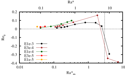
Figure 1: Surface equatorial jet amplitude as a function of $Ra_{m}^{\star}$ for several Ekman numbers.

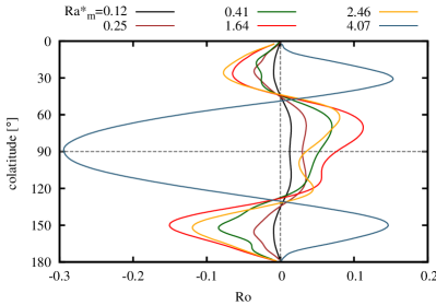
Figure 2: Surface zonal flow as function of colatitude for several Rayleigh numbers at an Ekman number of $E=10^{-3}$.

Fig. 2 shows the time averaged surface zonal flow profiles for increasing Rayleigh numbers at a fixed Ekman number of $E=10^{-3}$. At larger Rayleigh numbers, but before the transition around $Ra_{m}^{\star}\approx 3.0$, the zonal flow profiles show significant asymmetry with respect to the equator. This can be linked to the emergence of a global equatorial temperature asymmetry which drives an equatorial antisymmetric thermal wind structure (eq. 33). This scenario was first reported by Landeau and Aubert (2011) for simulations using rigid flow boundary conditions in order to model dynamos of terrestrial planets rather than the stress free conditions employed here. The symmetry breaking is promoted by volumetric heating and fixed flux thermal outer boundary conditions (Cao et al., 2014) but seems independent of the mechanical boundary conditions. Cao et al. (2014) report that the asymmetry is further promoted by the $Y_{20}$-shaped anomaly of the outer boundary heat flux when more heat is allowed to escape from the equatorial region, i.e. $q^{\star}<0$.

5 Inhomogeneous outer boundary heat flux

5.1 Thermal Winds and Zonal flows

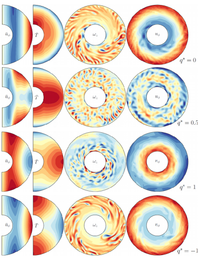
Figure 3: The two first columns show time and azimuthally averaged zonal flow and temperature. The two last columns show snapshots of equatorial cuts of $z$-vorticity and azimuthal flow.

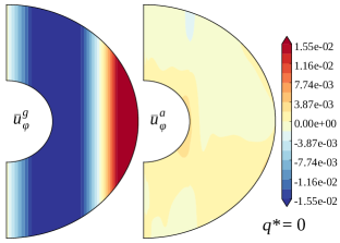
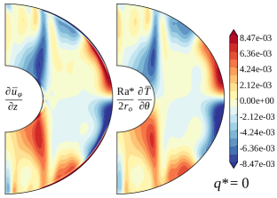
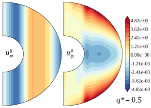
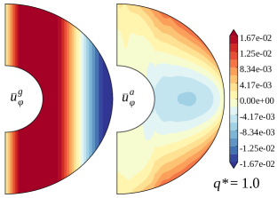
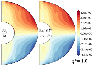
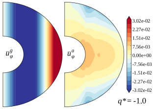
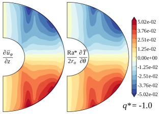
Figure 4: First and second columns show the geostrophic and ageostrophic part of the time-averaged zonal flow. The third and fourth column show the thermal wind balance. For some cases the contour levels in the plots of the geostrophic zonal flows are truncated in order to highlight the ageostrophic contribution since both share the same contour levels.

To investigate the interplay between geostrophic and ageostrophic zonal flows, we choose a reference case with homogeneous outer boundary heat flux and a moderate Rayleigh number where the zonal flow structure is strongly geostrophic and thermal winds play a minor role. We first consider a numerical model with $E=10^{-4}$ and $Ra^{\star}=0.2$ ($Ra^{\star}_{m}=0.082$). For this case this model yields a prograde equatorial zonal flow maintained by Reynolds stresses. Fig. 3 compares time and azimuthal average zonal flow and temperature for heat flux perturbation amplitudes $q^{\star}=0.5,1,-1$ with the reference case $q^{\star}=0$. The equatorial slices of $z$-vorticity and azimuthal flow illustrate the instantaneous structure. Fig. 4 shows the geostrophic and ageostrophic contributions of the time averaged zonal flow. The last two columns of this figure demonstrate that the ageostrophic part is indeed thermal wind related by illustrating the good agreement between left- and right-hand-side of the thermal wind balance eq. (33).

In the $q^{\star}=0$ reference case (top row of figs. 3, 4) the time-averaged zonal flow shows a strongly geostrophic structure with a prograde (retrograde) zonal flow at large (smaller) distances from the rotation axis $s$. The mostly radial isotherms (same figure, second column) confirm that latitudinal temperature gradients are too small to drive significant ageostrophic thermal winds. The snapshot of the equatorial $z$-vorticity shows mainly positive values and illustrates the consistent prograde tilt of the geostrophic columns.

The second rows of figs. 3, 4 show the solution for a moderate anomaly $q^{\star}=0.5$. At this value the heat flux at the equator (the pole) is half (1.5 times) the mean flux. Consequently the poles are cooled more efficiently by convection and a positive (negative) latitudinal temperature gradient is established in the northern (southern) hemisphere. The resulting thermal winds are retrograde in the equatorial region and prograde towards both poles. The geostropic zonal flow has also changed fundamentally and is now retrograde at large $s$, prograde at intermediate $s$ and again retrograde at small $s$. This seems roughly consistent with a change in the tilt of convective features illustrated in column three and four of fig. 3. Some retrograde tilted features can now be identified at large $s$ where the new retrograde zonal wind appeared.

If the perturbation amplitude is further increased to $q^{\star}=1$ thermal winds gain in amplitude while preserving a very similar structure. The geostrophic flows, however, have now reversed completely with a strong retrograde jet at the equator and wide prograde jets at smaller $s$. Convective flows (fig. 3, third row) are now rather weak closer to the outer boundary where the suppressed heat flux leaves a neutrally stratified hot equatorial region. Thermal winds are significantly stronger than for $q^{\star}=0.5$. The columns are now tilted dominantly in retrograde direction (see z-vorticity and $u_{\phi}$ snapshots in column 3 and 4 of figure 3). As we will further discuss below, this leads to a reversed direction of Reynolds stresses and consequently to a geostrophic zonal flow with retrograde equatorial and prograde inner jet. Whereas the influence of an increased $q^{\star}$ on the thermal wind is as expected, the influence on the tilt and thus the geostrophic zonal flow direction comes as a surprise. Since the Reynolds stress driven geostrophic zonal flow component is once more clearly dominant, the relative vertical variation is weaker than for the $q^{\star}=0.5$ model.

We also tested the case $q^{\star}=-1$ where the heat flux is enhanced in the equatorial region but reduced towards the poles. The last columns in figs. 3 and 4 show that the thermal wind is as strong as in the $q^{\star}=1$ simulations but, as expected, simply has reversed its sign. The geostrophic zonal flows increase in amplitude but retain their structure. Likewise, convective features have a similar distribution and the same tilt direction as in the $q^{\star}=0$ reference case. However, the Reynolds stresses are more efficient as demonstrated by the non-axisymmetric flow correlation listed in tab. 1 and therefore drives stronger geostrophic zonal flows.

Fig. 5 shows the changes of the surface zonal flow patterns when $q^{\star}$ is increased. If the non-homogeneous outer boundary condition would only drive thermal wind but leave the geostrophic zonal flow largely unaffected, the surface flow profile would remain unchanged at the equator and become more prograde at mid to high latitudes. The high latitude retrograde jets would be weakened or reversed, while the low-latitude prograde jet would be intensified except directly at the equator.

However, due to the fact that the geostrophic winds also change drastically, the behaviour appears very different. The reduction and ultimately reversal of Reynolds stress driven geostrophic zonal flows starts at the equator as $q^{\star}$ increases and propagates inwards. The equatorial jet therefore first develops a dimple or minimum around the equator before it turns retrograde at even higher $q^{\star}$. The dimple deepens with increasing $q^{\star}$ and is reminiscent of a similar feature in Jupiter’s main prograde jet.

At $q^{\star}=0.4$ the equatorial zonal flow practically vanishes at the outer boundary while stronger perturbations promote increasingly retrograde equatorial jets. The respective flow profiles are then similarly shaped to the ones observed for Neptune and Uranus (Aurnou et al., 2007, e.g.). For an anomaly with negative sign ($q^{\star}=-1$) the structure is similar to the homogeneous ($q^{\star}=0$)-model but with twice the amplitude.

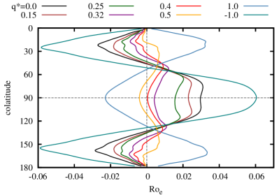
Figure 5: Surface zonal flow structure for several perturbations amplitude $q^{\star}$. From $q^{\star}\simeq 0.5$ the thermal forcing reverts the equatorial jet from prograde to retrograde. Parameters: $E=10^{-4},\,Ra^{\star}=0.2,\,Pr=1$.

5.2 Force Balance

q	0	0.5	1	-1
$Re_{\overline{\phi}}$	364.43	58.84	335.22	619.61
$Re_{\overline{s}}$	0.878	0.857	1.751	0.885
$Re_{\phi^{\prime}}$	78.50	67.81	81.72	96.11
$Re_{s^{\prime}}$	56.12	63.08	56.73	55.99
$\cal{RS}$	1054.1	65.59	731.7	1569.6
$\cal{AD}$	10.1	6.74	113.1	8.13

Table 1: Several flow properties for the four study cases with $q=0$, 0.5, 1, and -1. The individual Reynolds numbers are calculated for the axisymmetric (overbar) and non-axisymmetric (primed) flows along azimuth ($\phi$) and cylindrical radial (s).

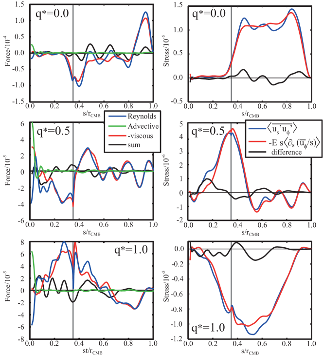
Figure 6: The left column shows the z-averaged force due to Reynolds stress (blue), the advective force (green), minus the viscous force (red), and the sum of the two forces (black) for three of the four cases depicted in fig. 3. The right column shows respective z-averaged contributions to the balance between the Reynolds stress (blue) and the viscous stress (red) according to eqn. 29. The vertical black lines denote the tangent cylinder.

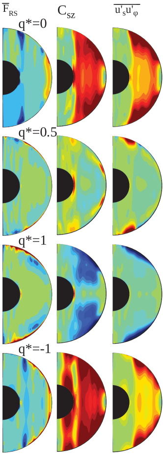
Figure 7: Time averaged axisymmetric azimuthal maps of Reynolds stress convergence, correlation $C_{s\phi}$ and Reynolds stress ($\overline{u_{\phi}^{\prime}u_{s}^{\prime}}$) for the four selected cases at different $q^{\star}$ values already depicted in fig. 3. Contours for the first and second columns have been chosen to individually highlight the structure. The correlation shown in column two varies between $-0.5$ and $0.5$.

Fig. 6 shows the $z$ and time averaged zonal force balance due to Reynolds stress convergence, advective force and viscous force (left column) for the cases at $Ra^{\star}=0.2$ and $E=10^{-4}$ already discussed in section 5.1. As suggested in tab. 1 the advective force due to meridional circulation is negligible for all cases. The two dominant terms in the stress balance (29) are displayed in the right column. Results for $q^{\star}=-1$ are not shown since they are very similar to that for $q^{\star}=0$. Note that the Reynolds stress and viscous contributions do not balance perfectly mostly because we have not averaged long enough in time. Fig. 7 compares the time averaged zonal Reynolds stress convergence, correlation $C_{s\phi}$, and the azimuthally averaged nonlinear product $\overline{u_{s}^{\prime}u_{\phi}^{\prime}}$, e.g. the Reynolds stress. The correlation coefficient $C_{s\phi}$ is defined as

$$C_{s\phi}(s,z)=\frac{\overline{u_{s}^{\prime}u_{\phi}^{\prime}}}{\left(\overline{{u_{s}^{\prime}}^{2}}\overline{{u_{\phi}^{\prime}}^{2}}\right)^{1/2}}\ .$$ (34)

For a homogeneous outer boundary heat flux, positive (negative) Reynolds stress convergence close to the outer boundary (tangent cylinder) is responsible for driving the prograde equatorial and retrograde inner zonal jets (first columns in fig. 6 and fig. 7). The correlation $C_{s\phi}$ is strongly positive outside the tangent cylinder due to the generally prograde tilt of the convective features here (second column in fig. 7). The region close to the outer boundary contributes more to $\overline{u_{s}^{\prime}u_{\phi}^{\prime}}$ and thus to the Reynolds stress because of higher $u_{\phi}^{\prime}$ and $u_{s}^{\prime}$ amplitudes (column three in fig. 7). The $z$-average $\left\langle\overline{u_{s}^{\prime}u_{\phi}^{\prime}}\right\rangle$ (second column in fig. 6) shows a pronounced positive hump between the tangent cylinder and the outer boundary equator. Steep gradients close to these two boundaries translate into the two dominating Reynolds stress convergence features.

At $q^{\star}=0.5$ the correlation and thus the Reynolds stress is very low. The positive hump in $\left\langle\overline{u_{s}^{\prime}u_{\phi}^{\prime}}\right\rangle$ is now located at the tangent cylinder, resulting in prograde (retrograde) Reynolds stress convergence attached to the inside (outside) of the TC. Fig. 7 illustrates that the reason is the strong concentration of non-axisymmetric flow components close to where the TC touches the outer boundary.

At $q^{\star}=1$ the correlation $C_{s\phi}(s,z)$ is once again generally strong outside the tangent cylinder except for a region around the equatorial plane. The sign is now negative, however, due to the retrograde tilt of non-axisymmetric convective features.

Once more, $\overline{u_{s}^{\prime}u_{\phi}^{\prime}}$ and thus the Reynolds stress convergence are strongest closer to the outer boundary and at mid to higher latitudes. The negative hump in $\left\langle\overline{u_{s}^{\prime}u_{\phi}^{\prime}}\right\rangle$ reaches inside the tangent cylinder, leading to a strong positive force due to Reynolds stress there.

As already discussed above, the test case for $q^{\star}=-1$ is generally very similar to the reference case $q^{\star}=0$. However, the positive correlation now also stretches inside the tangent cylinder while the non-axisymmetric flow is somewhat stronger promoted at lower latitudes. The combination of both results in a Reynolds stress pattern similar to that at $q^{\star}=0$.

The primary flow component driven by the boundary inhomogeneity is the thermal wind. However, the advective force via which the thermal wind could directly contribute to drive geostrophic zonal flows remains very small for all the cases explored here ( table 1). The Reynolds stress and correlation analysis confirm what we had already anticipated in section 3: the zonal flow inversion is related to the global change in the sign of the correlation $C_{s\phi}$ which in turn is caused by the inversion of the tilt. In the next section we discuss which mechanisms could be responsible for changing the tilt. Other changes in the non-axisymmetric convective flow are also pronounced but mostly concern the distribution of Reynolds stress and not its general direction. For example, we find an unexpected strong contribution of equatorial antisymmetric, non-axisymmetric convective flows at $q^{\star}>0.5$.

6 Changing the tilt

The tilt of convective features and the related zonal flow generation by Reynolds stresses has been extensively discussed in the literature and we refer to Busse (2002) and Takehiro (2008) for overviews. In fast rotating spherical shells convection sets in as thermal Rossby waves that have the form of geostrophic columns aligned with the rotation axis (Busse, 1970). These waves drift in azimuthal direction with a velocity that is determined by the height change of the container. When the height $h$ decreases with the cylindrical radius $s$, as is the case outside the tangent cylinder, the waves drift in prograde direction. A tilted or spiralling form in the $s$-direction is assumed when the phase $\Phi_{0}$ of the wave depends on $s$. When $\partial\Phi_{0}/\partial s>0$ the columns are tilted in prograde direction.

Busse and Hood (1982) suggested that the tilting direction of the convective columns is controlled by the curvature of the confining walls. They study a cylindrical annulus with curved upper and lower caps, a system that captures the essence of the thermal Rossby waves while reducing the impact of meridional circulation. Using asymptotic analysis and laboratory experiments they show that convex caps similar to those in spherical shells yield drifting thermal Rossby waves that tilt in prograde direction. The tilt is reversed for concave caps. Their asymptotic analysis confirms that the $s$-gradients of $\Phi_{0}$ indeed depends directly on the boundary curvature in the way indicated by the experiments. A simple argument discussed by (Busse, 2002) links the phase to the potential drift speed of the wave. Since $\partial h/\partial s$ increases with $s$ outside the tangent cylinder the wave should drift faster at larger than at smaller $s$. The solution which drifts with only one velocity adapts to this situation by assuming an $s$-dependent phase $\Phi_{0}(s)$. The actual mechanism that leads to the tilt was discussed later by Takehiro (2008)

Busse and Hood (1982) and Busse (2002) discuss various issues that can influence the phase relation $\Phi_{0}(s)$. One example is the onset of a secondary instability with the same azimuthal wave number as the primary instability but a different radial dependence. Differences in the heating mode are another alternative first mentioned by Busse and Hood (1982) and later explored in more detail by Takehiro (2008). Using a simplified annulus system, he showed that the typical prograde tilt results when energy is mostly fed into the system close to the inner boundary but has to travel outward to larger radii where most of the energy is dissipated. When the locations of primary energy input and dissipation are reversed, however, the tilt changes to retrograde. He concludes that the propagation of the Rossby wave in $s$-direction is the key physical process that controls the tilt direction. The applicability of this theory was extended towards spherical systems by Takehiro (2010).

Fig. 8 compares the energy input $Ra^{\star}r/r_{o}u^{\prime}_{r}T$ with non-axisymmetric energy diffusion $\mbox{$\mathchoice{\mbox{\boldmath$\displaystyle u^{\prime}$}}{\mbox{\boldmath$\textstyle u^{\prime}$}}{\mbox{\boldmath$\scriptstyle u^{\prime}$}}{\mbox{\boldmath$\scriptscriptstyle u^{\prime}$}}$}\cdot(\nabla^{2}\mbox{$\mathchoice{\mbox{\boldmath$\displaystyle u$}}{\mbox{\boldmath$\textstyle u$}}{\mbox{\boldmath$\scriptstyle u$}}{\mbox{\boldmath$\scriptscriptstyle u$}}$})$ integrated over geostrophic cylinders and over time for the different cases discussed above. Both terms result from multiplying the Navier-Stokes equation (3) with the non-axisymmetric velocity $\textstyle u^{\prime}$. When $q^{\star}$ is increased the energy input moves progressively away from the outer boundary and is clearly concentrated at the tangent cylinder for $q^{\star}=1.0$. Energy input and diffusion always have very similar distributions making it impossible to deduce a potential Rossby wave propagation in $s$-direction. As the zonal flow is reversed consistently with the also reversed Reynolds stress for $q^{\star}=1.0$, a misalignment of energy input and diffusion should be visible, what is clearly not the case. Hence the switch from outward to inward propagation on increasing $q^{\star}$ is not explainable with this rationale.

Following the line of arguments by (Busse and Hood, 1982) and (Busse, 2002) the tilt change could also be explained when the region inside the tangent cylinder becomes more important for determining the Rossby wave properties. The inverted height gradient $\partial h/\partial s$ in this region could explain the change in Rossby wave drift and tilt. However, while fig. 8 certainly suggest that the region inside the tangent cylinder becomes more important on increasing $q^{\star}$, the total energy input is still dominated by the region outside the tangent cylinder even at $q^{\star}=1$.

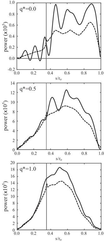
Figure 8: Energy input (solid) and diffusion (dashed) of non-axisymmetric kinetic energy integrated over geostrophic cylinders and averaged over times for the three selected cases at $Ra^{\star}=0.2$ and $E=10^{-4}$. The vertical grey lines denote the tangent cylinder.

Obviously, neither the curvature argument invoked by Busse and Hood (1982) nor the Rossby wave reasoning proposed by Takehiro (2008, 2010) explain the change in tilt in an obvious way. This may not be surprising since both assume geostrophic fundamental solutions. While the $q^{\star}=0$ cases may still be more or less compliant with the assumption of dominant geostrophy, this changes once the non-homogeneous boundary condition becomes more influential. The decisively non-geostrophic solutions found at $q^{\star}\approx 0.5$ may require a completely different approach.

It remains to be said that the tilt is generally compatible with the geostrophic flow directions in the sense that an, for whatever reason, inverted geostrophic flow pattern would also invert the tilt.

The simple reason is the twisting that any zonal shear exerts on the columns. Busse (2002) suggest that the tilt direction could be determined by a run-away effect he called the mean flow instability. Suppose, that a system with an undecided columnar tilt is subjected to a small initial zonal wind shear which could be the result of an instability. The shear most likely tilts the columns, spawns Reynolds stresses and thereby amplifies itself. This run-away effect would ultimately stop when viscous and Reynolds stresses balance. The effect of the initial zonal wind needs to be strong enough to overcome any other potentially tilting mechanism discussed above. A small noise fluctuation would likely not suffice.

7 Parameter Dependence

7.1 Anomaly amplitude

To complete and generalise the picture outlined above, we investigate several diagnostic quantities as a function of the anomaly amplitude $q^{\star}$. Besides the average Reynolds stress $\cal RS$ (eq. 30) we quantify the zonal wind geostrophy with an rms $z$-length scale following Gastine and Wicht (2012)

$$\ell_{z}=\frac{\left[\overline{u}_{\phi}\right]_{\mathrm{rms}}}{\left[\partial\overline{u}_{\phi}/\partial z\right]_{\mathrm{rms}}}\;\;.$$ (35)

The impact of the imposed heat flux boundary pattern on the deep temperature structure is measured by the globally averaged latitudinal gradient of the axisymmetric temperature:

$$\Delta_{\Theta}=\left[\frac{\partial\overline{T}}{\partial\theta}\right]_{\mathrm{rms}}.$$ (36)

The kinetic energy of geostrophic and ageostrophic zonal flows quantify the importance of the respective contributions:

$$\left\langle E\right\rangle=\frac{1}{2V}\int{\color[rgb]{0.0,0.0,0.0}\left\langle\overline{u}_{\phi}\right\rangle^{2}}dV\;\;,$$ (37)

$$\left\{E\right\}=\frac{1}{2V}\int{\color[rgb]{0.0,0.0,0.0}\left\{\overline{u}_{\phi}\right\}^{2}}dV\;\;,$$ (38)

where $V$ is the volume of the spherical shell.

Fig. 9 shows the variation of these different diagnostic quantities with increasing $q^{\star}$. The first panel of fig. 9 demonstrates the clear correlation between the equatorial jet velocity and the Reynolds stress ${\cal RS}$. This once more highlights that the Reynolds stress drives the geostrophic zonal winds and that its inversion correlates with the change in the zonal flow direction.

The length scale $\ell_{z}$ and thus geostrophy first decreases with growing thermal wind but recovers and saturates once the geostrophic wind direction has reversed. Not surprisingly, $\Delta_{\Theta}$ increases roughly linearly with $q^{\star}$ as does the rms amplitude of ageostrophic mostly thermal wind related zonal flows measured by $\left\{E\right\}$ in Fig. 9c. The geostrophic contribution, however, has a minimum around the zonal flow reversal and clearly dominates at $q^{\star}=0$ and $q^{\star}=1$. Once the convective columns have changed their tilt Reynolds stresses efficiently drive the geostrophic zonal flows.

Interestingly, there is a hysteretic behaviour between increasing and decreasing $q^{\star}$ that is also found in the average geostrophy of the zonal flow (Fig. 9b). The hysteretic behaviour can be found for all measures involving the geostrophic zonal winds, which suggests that the zonal flow direction indeed plays a role in determining the tilt. Whichever mechanism ultimately changes the tilt has to overcome the tilt direction promoted by the zonal wind shear. A similar hysteretic behaviour is also reported by Gastine et al. (2014b) who study the zonal flow reversal happening at large Rayleigh numbers for Rossby numbers around one.

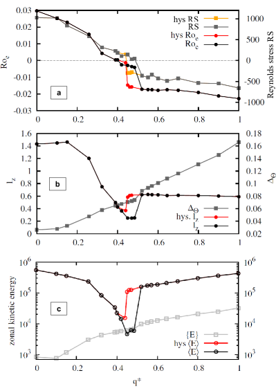
Figure 9: Various flow properties as a function of the heat flux perturbation amplitude $q^{\star}$: (a) zonal Rossby number at the equator $Ro_{e}$ and mean Reynolds stress; (b) $\ell_{z}$ and mean latitudinal gradient of axisymmetric temperature; (c) kinetic energy of zonal flows for geostrophic and ageostrophic flow contributions. The orange and red profiles are calculated with decreasing $q^{\star}$ to visualise the hysteretic character.

7.2 Rayleigh and Ekman number

Rayleigh and Ekman numbers may have a crucial impact on the zonal flow direction and amplitude. In the rotation-dominated convection regime, the Rayleigh number first increases with Rayleigh number simply because the convective flow amplitudes grow. For larger $Ra^{\star}$ Reynolds stresses decrease because the correlation between non-axisymmetric flow contributions is gradually lost (Christensen, 2002; Gastine and Wicht, 2012).

On the other hand, $Ra^{\star}$ is the only parameter in the thermal wind balance (eq. 33) and therefore controls the ageostrophic zonal flows. To explore the parameter dependence, we compute several numerical models spanning the range from $Ra^{\star}=0.1$ to $Ra^{\star}=0.8$ with a fixed Ekman number of $E=10^{-4}$. Figure 10 shows how the equatorial zonal wind changes as $q^{\star}$ is increased. In general, the amplitude of the equatorial jet for both directions scales with $Ra^{\star}$. The transition of the direction happens earlier for smaller $Ra^{\star}$. When the zonal winds are weaker to start with, the boundary induced effect seems to have an easier task to change the direction.

In the curve for $Ra^{\star}=0.2$, there is a pronounced jump in velocity when the jet is inverted as already discussed above. A similar jump is expected to happen for the other cases. Relying on Reynolds stresses, the transition is a non-linear phenomenon and therefore particularly sensitive to flow amplitudes and thus to Rayleigh numbers. More vigorous convection at higher $Ra^{\star}$ leads to a more abrupt transition.

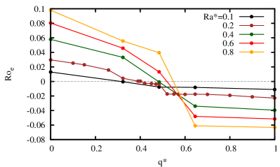
Figure 10: Equatorial zonal flow $Ro_{e}$ at the outer boundary as a function of the perturbation amplitude $q^{\star}$ for 5 different Rayleigh numbers.

To investigate the impact of a smaller Ekman numbers $E$, we adjust the Rayleigh number to provide roughly the same $Ro_{e}$ for the homogeneous reference case for all Ekman numbers. The ($E=10^{-4}$)-model served as a reference and we adjusted the $Ra^{\star}$-values accordingly.

Fig. 11 shows $Ro_{e}$ as a function of $q^{\star}$ for 5 different Ekman numbers spanning the range from $E=10^{-3}$ to $E=10^{-5}$. Higher Ekman numbers result in stronger reverted zonal flows at the equator, i.e. higher $Ro_{e}$. Smaller Ekman numbers promote more geostrophic flows and higher perturbation amplitudes are required to overcome this constraint. While $Ro_{e}(q^{\star}=0)$ is similar for all combinations of $Ra^{\star}$ and $E$ in Fig. 11, $Ra^{\star}$ decreases from $0.6$ at $E=10^{-3}$ to $0.08$ at $E=10^{-5}$. As the zonal flow amplitude in the inverted jet regime increases with $Ra^{\star}$ (Fig. 10), the low Ekman number cases yield weaker equatorial jets. However, given the crossover between cases for $E=3\cdot 10^{-5}$ (red) and $E=10^{-5}$ (orange) there might be another effect not understood so far.

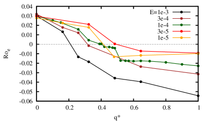
Figure 11: Equatorial zonal flow $Ro_{e}$ at the outer boundary as a function of the perturbation amplitude $q^{\star}$ for 5 different Ekman numbers.

8 Discussion

We have shown that imposing an outer boundary heat flux pattern that allows more heat to escape at higher latitudes while suppressing convection in the equatorial region can revert the geostrophic flow system. Strongly retrograde equatorial jets like those observed on Uranus or Neptune are the consequence. The process is fairly general and happens at different Rayleigh and Ekman numbers when the amplitude $q^{\star}$ of the imposed heat flux variation reaches about 50% of the mean heat flux.

The imposed boundary condition is primarily responsible for a deep reaching temperature anomaly that mirrors the imposed pattern: the equatorial region remains hot while mid to high latitude regions are cooled more efficiently by convection. Strong thermal winds are the direct consequence of the respective latitudinal temperature gradient and as expected, these thermal wind speeds increase with $q^{\star}$. However, the effects on the geostrophic flow, i.e.  reversal and re-amplification for large enough positive $q^{\star}$ as well as the boost for negative $q^{\star}$ are indeed unforeseen.

An analysis of the force balance has shown that the geostrophic zonal flows are always driven by Reynolds stresses, i.e. by a statistical correlation of non-axisymmetric flow contributions. The axisymmetric thermal wind has therefore no direct impact on the flow reversal. However, our analysis demonstrates the reversal correlates with a change in the tilt of convective columns. This is perhaps not surprising, since this tilt is always fundamental in establishing geostrophic Reynolds stresses, but it offers the potential explanation: the imposed boundary conditions could actually affect the tilt.

Unfortunately, we have not found a convincing connection so far and may also face a chicken and egg problem here since the shear related to zonal flows can by itself determine the tilt of convective columns. Sure enough, Reynolds stress and columnar tilt are always consistent in our simulations. The typical concepts for explaining the tilt and geostrophic zonal flow, such as the Rossby wave propagation (Busse and Hood, 1982; Takehiro, 2008), can not explain the numerical results.

It seems tempting to apply our numerical results to the giant planets bearing the question what would be a reasonable outer boundary heat flux pattern. Here we consider the possible effect of intense solar irradiation. The heat flux from the deeper regions is likely reduced where the solar incident flux heats the outermost atmosphere more effectively. The details of this process depend on e.g., radiative transfer, albedo variations, convection in the weather layer and chemical processes. However, here we take a simpler approach and consider only the lateral distribution of the mean solar irradiation. Relevant here is the temporal mean of the solar irradiation over time scales required to alter zonal flows.

Our numerical simulations, but also Jupiter’s zonal flow structure suggest that the zonal winds generally change very slowly (Vasavada and Showman, 2005). Since the zonal flows are predominantly geostrophic any change requires to accelerate a significant fraction of the total planetary mass and can therefore only be slow. The associated time scales $\tau_{ZF}$ can be estimated via the driving Reynolds stresses

$$\frac{\partial\overline{v}_{\phi}}{\partial t}\approx\frac{\overline{v}_{\phi}}{\tau_{ZF}}\approx\overline{\mathchoice{\mbox{\boldmath$\displaystyle v$}}{\mbox{\boldmath$\textstyle v$}}{\mbox{\boldmath$\scriptstyle v$}}{\mbox{\boldmath$\scriptscriptstyle v$}}_{c}\cdot\nabla\mathchoice{\mbox{\boldmath$\displaystyle v$}}{\mbox{\boldmath$\textstyle v$}}{\mbox{\boldmath$\scriptstyle v$}}{\mbox{\boldmath$\scriptscriptstyle v$}}_{c}}\approx C\frac{v_{c}^{2}}{d_{ZF}}\ ,$$ (39)

yielding

$$\tau_{zf}=\frac{\overline{v}_{\phi}\,d_{ZF}}{C\,v_{c}^{2}}\ .$$ (40)

Here $d_{ZF}$ is the width of the zonal flow jet and $C$ the mean correlation. $\overline{v}_{\phi}$ and $v_{c}$ are the dimensional flow speeds of peak azimuthal and convective flow.

Assuming a perfect correlation $C=1$ provides an upper bound. Using for example Jupiter’s zonal flow maximum of $\overline{v}_{\phi}=150\,\mathrm{m/s}$ observed by the Galileo entry probe, the width of the equatorial jet $d_{ZF}=2.1\cdot 10^{6}\,\mathrm{m}$ and an estimate for the convective flow speeds of $v_{c}=1\,\mathrm{cm/s}$ (Jones, 2014; Gastine et al., 2014a) yields $\tau_{ZF}=0.1\,\mathrm{Myr}$ or $8400$ orbital (sideric) revolutions. Equivalent estimates for Saturn, Neptune and Uranus can be found in tab. 2.

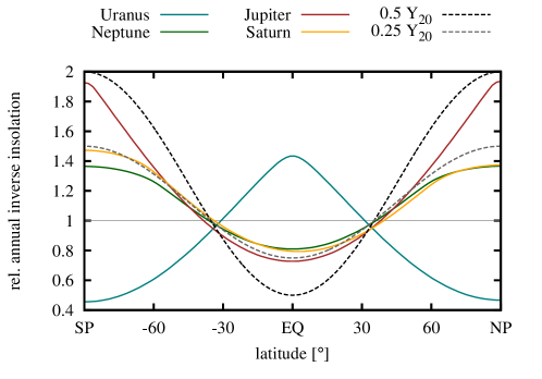
Figure 12: Inverse normalised annual solar irradiation as a function of planetary latitude atop the atmospheres of the four giant planets and $Y_{20}$-patterns.

This implies that when calculating the impact of solar irradiation we have to consider the average over a sideric orbit. Fig. 12 shows the respective inverse latitudinal insolation profiles for Jupiter, Saturn, Uranus and Neptune in comparison to $Y_{20}$ patterns as used in the study. Those are found by averaging daily irradiation pattern for each planet while taking orbital properties, such as obliquity and eccentricity, into account (accordingly to van Hemelrijck (1982)). The profiles for Jupiter, Saturn and Neptune show an enhanced insolation (reduced internal heat flux) in the equatorial region. Due to the large obliquity, however, the pattern for Uranus is flipped since the high polar irradiation during summer dominates the annual mean (van Hemelrijck, 1988).

Observations suggest that the latitudinal total emission profiles of all four giant planets are rather flat (Ingersoll, 1976; Pearl et al., 1990; Pearl and Conrath, 1991; Soderlund et al., 2013). Consequently the solar irradiation must be compensated either by a latitudinal variation of the internal heat flux (Aurnou et al., 2008) or by equilibrating processes in the upper atmosphere. Adopting the former scenario allows to estimate the internal flux by simply inverting the irradiation profiles. Fig. 12 shows that the $Y_{20}$-pattern with variable $q^{\star}$ indeed provides a reasonable match for Jupiter, Saturn and Neptune. Uranus insolation however suggests a negative $q^{\star}$ value.

For Jupiter and Saturn the internal heat flux is roughly equal to the absorbed insolation (Guillot and Gautier, 2007). Since the internal heat flux is also hugely superadiabatic, we can directly translate the inverse insolation pattern into a $q^{\star}$-value. Fig. 12 shows that for Jupiter a $q^{\star}\approx 0.5$ is required to compensate the insolation pattern. Our numerical simulations suggest that a mild heat flux variation of $q^{\star}=0.3$ generates a dimple of the equatorial prograde jet similar to Jupiter’s main belt structure (see fig. 5). Equilibrating convection within the upper atmosphere may possibly reduce the effective $q^{\star}$ for Jupiter’s deeper convection. For Saturn our approximation suggests $q^{\star}\approx 0.25$, but since no dimple in the equatorial main jet has been observed the insolation flux maybe almost entirely compensated by upper atmosphere circulations.

The insolation pattern also suggests $q^{\star}\approx 0.25$ for Neptune. Since the internal heat flux is $50\%$ larger than the insolation flux, the effective $q^{\star}$ reduces to ca. 0.15 (Guillot and Gautier, 2007). This seems insufficient to create the inverse zonal flow patterns observed for Neptune. Our simulations at least require $q^{\star}=0.5$ for inverse zonal flow directions and possibly much larger values to also reach appropriate flow speeds.

However, for Uranus the peculiar insolation pattern exclude our proposed mechanism for explaining the jet directions. The fact that the emitted flux is almost equal to the absorbed flux means that the minuscule internal flux can not be the reason for the roughly homogeneous emission profile. At least for Uranus the convective processes within the upper atmosphere must eradicate any horizontal insolation gradient.

Alternative attempts to explain the inverse differential rotation on the ice giants had to invoke the angular momentum mixing found at large Rayleigh numbers (Aurnou et al., 2007; Gastine et al., 2013; Soderlund et al., 2013).

planet	$\overline{v}_{\phi}$ [m/s]	$d_{ZF}$ [$10^{6}$ m]	$\tau_{ZF}$ [Myr]	$\tau_{sid}/\tau_{ZF}$
Jupiter	150	2.1	0.1	$8.4\cdot 10^{3}$
Saturn	450	6.2	0.87	$2.9\cdot 10^{4}$
Uranus	200	3.0	0.19	$2.3\cdot 10^{3}$
Neptune	300	7.9	0.75	$8.1\cdot 10^{3}$

Table 2: Characteristic time scales of zonal flow variations $\tau_{ZF}$ based on eq. 40 in comparison to a sideric period $\tau_{sid}$. The jet width $d_{ZF}$ is estimated by the width of the equatorial jet, $v_{\phi}$ is the peak equatorial jet.

Even though the proposed mechanism may not apply to the atmosphere of the planets in the solar system it is nevertheless an interesting hydrodynamic effect that requires further investigation. It is interesting that the common theories of differential rotation in rapidly rotating spherical shell convection fail to explain the effect of thermal inhomogeneities applied at the outer boundary.

References

- Amit et al. (2011) Amit, H., Christensen, U. R., Langlais, B., Nov. 2011. The influence of degree-1 mantle heterogeneity on the past dynamo of Mars. Physics of the Earth and Planetary Interiors 189, 63–79.
- Aubert (2005) Aubert, J., Oct. 2005. Steady zonal flows in spherical shell dynamos. Journal of Fluid Mechanics 542, 53–67.
- Aurnou et al. (2008) Aurnou, J., Heimpel, M., Allen, L., King, E., Wicht, J., Jun. 2008. Convective heat transfer and the pattern of thermal emission on the gas giants. Geophysical Journal International 173, 793–801.
- Aurnou et al. (2007) Aurnou, J., Heimpel, M., Wicht, J., Sep. 2007. The effects of vigorous mixing in a convective model of zonal flow on the ice giants. Icarus190, 110–126.
- Aurnou and Aubert (2011) Aurnou, J. M., Aubert, J., Aug. 2011. End-member models of boundary-modulated convective dynamos. Physics of the Earth and Planetary Interiors 187, 353–363.
- Busse (1970) Busse, F. H., 1970. Thermal instabilities in rapidly rotating systems. Journal of Fluid Mechanics 44, 441–460.
- Busse (1976) Busse, F. H., Oct. 1976. A simple model of convection in the Jovian atmosphere. Icarus29, 255–260.
- Busse (1983) Busse, F. H., 1983. A model of mean zonal flows in the major planets. Geophysical and Astrophysical Fluid Dynamics 23, 153–174.
- Busse (2002) Busse, F. H., Apr. 2002. Convective flows in rapidly rotating spheres and their dynamo action. Physics of Fluids 14, 1301–1314.
- Busse and Hood (1982) Busse, F. H., Hood, L. L., 1982. Differential rotation driven by convection in a rapidly rotating annulus. Geophysical and Astrophysical Fluid Dynamics 21, 59–74.
- Cao et al. (2014) Cao, H., Aurnou, J. M., Wicht, J., Dietrich, W., Soderlund, K. M., Russell, C. T., Jun. 2014. A dynamo explanation for Mercury’s anomalous magnetic field. Geophys. Res. Lett.41, 4127–4134.
- Cho and Polvani (1996) Cho, J. Y.-K., Polvani, L. M., Jun. 1996. The emergence of jets and vortices in freely evolving, shallow-water turbulence on a sphere. Physics of Fluids 8, 1531–1552.
- Christensen (2001) Christensen, U. R., Jul. 2001. Zonal flow driven by deep convection in the major planets. Geophys. Res. Lett.28, 2553–2556.
- Christensen (2002) Christensen, U. R., Nov. 2002. Zonal flow driven by strongly supercritical convection in rotating spherical shells. Journal of Fluid Mechanics 470, 115–133.
- Christensen and Wicht (2007) Christensen, U. R., Wicht, J., 2007. Numerical Dynamo simulations. In: Olson, P. (Ed.), Treatise on Geophysics Volume 8: Core Dynamics. Treatise on Geophysics. Elsevier, pp. 245–282.
- Dietrich et al. (2016) Dietrich, W., Hori, K., Wicht, J., Feb. 2016. Core flows and heat transfer induced by inhomogeneous cooling with sub- and supercritical convection. Physics of the Earth and Planetary Interiors 251, 36–51.
- Dietrich and Wicht (2013) Dietrich, W., Wicht, J., Apr. 2013. A hemispherical dynamo model: Implications for the Martian crustal magnetization. Physics of the Earth and Planetary Interiors 217, 10–21.
- Dietrich et al. (2015) Dietrich, W., Wicht, J., Hori, K., Dec. 2015. Effect of width, amplitude, and position of a core mantle boundary hot spot on core convection and dynamo action. Progress in Earth and Planetary Science 2, 35.
- Gastine et al. (2014a) Gastine, T., Heimpel, M., Wicht, J., Jul. 2014a. Zonal flow scaling in rapidly-rotating compressible convection. Physics of the Earth and Planetary Interiors 232, 36–50.
- Gastine and Wicht (2012) Gastine, T., Wicht, J., May 2012. Effects of compressibility on driving zonal flow in gas giants. Icarus219, 428–442.
- Gastine et al. (2013) Gastine, T., Wicht, J., Aurnou, J. M., Jul. 2013. Zonal flow regimes in rotating anelastic spherical shells: An application to giant planets. Icarus225, 156–172.
- Gastine et al. (2014b) Gastine, T., Yadav, R. K., Morin, J., Reiners, A., Wicht, J., Feb. 2014b. From solar-like to antisolar differential rotation in cool stars. MNRAS438, L76–L80.
- Gilman and Foukal (1979) Gilman, P. A., Foukal, P. V., May 1979. Angular velocity gradients in the solar convection zone. ApJ229, 1179–1185.
- Glatzmaier and Gilman (1982) Glatzmaier, G. A., Gilman, P. A., May 1982. Compressible convection in a rotating spherical shell. V - Induced differential rotation and meridional circulation. ApJ256, 316–330.
- Guillot and Gautier (2007) Guillot, T., Gautier, D., 2007. Giant Planets. In: Spohn, T. (Ed.), Treatise on Geophysics Volume 10: Planets and Moons. Treatise on Geophysics. Elsevier, pp. 439–464.
- Hammel et al. (2005) Hammel, H. B., de Pater, I., Gibbard, S., Lockwood, G. W., Rages, K., Jun. 2005. Uranus in 2003: Zonal winds, banded structure, and discrete features. Icarus175, 534–545.
- Heimpel et al. (2005) Heimpel, M., Aurnou, J., Wicht, J., Nov. 2005. Simulation of equatorial and high-latitude jets on Jupiter in a deep convection model. Nature438, 193–196.
- Ingersoll (1976) Ingersoll, A. P., Oct. 1976. Pioneer 10 and 11 observations and the dynamics of Jupiter’s atmosphere. Icarus29, 245–252.
- Ingersoll et al. (1975) Ingersoll, A. P., Muench, G., Neugebauer, G., Diner, D. J., Orton, G. S., Schupler, B., Schroeder, M., Chase, S. C., Ruiz, R. D., Trafton, L. M., May 1975. Pioneer 11 infrared radiometer experiment - The global heat balance of Jupiter. Science 188, 472.
- Jones (2014) Jones, C. A., Oct. 2014. A dynamo model of Jupiter’s magnetic field. Icarus241, 148–159.
- Landeau and Aubert (2011) Landeau, M., Aubert, J., Apr. 2011. Equatorially asymmetric convection inducing a hemispherical magnetic field in rotating spheres and implications for the past martian dynamo. Physics of the Earth and Planetary Interiors 185, 61–73.
- Lian and Showman (2010) Lian, Y., Showman, A. P., May 2010. Generation of equatorial jets by large-scale latent heating on the giant planets. Icarus207, 373–393.
- Liu and Schneider (2011) Liu, J., Schneider, T., Nov. 2011. Convective Generation of Equatorial Superrotation in Planetary Atmospheres. Journal of Atmospheric Sciences 68, 2742–2756.
- Miesch et al. (2006) Miesch, M. S., Brun, A. S., Toomre, J., Apr. 2006. Solar Differential Rotation Influenced by Latitudinal Entropy Variations in the Tachocline. ApJ641, 618–625.
- Pearl and Conrath (1991) Pearl, J. C., Conrath, B. J., 1991. The albedo, effective temperature, and energy balance of Neptune, as determined from Voyager data. Journal of Geophysical Research Supplement 96, null.
- Pearl et al. (1990) Pearl, J. C., Conrath, B. J., Hanel, R. A., Pirraglia, J. A., Mar. 1990. The albedo, effective temperature, and energy balance of Uranus, as determined from Voyager IRIS data. Icarus84, 12–28.
- Pirraglia (1984) Pirraglia, J. A., Aug. 1984. Meridional energy balance of Jupiter. Icarus59, 169–176.
- Plaut et al. (2008) Plaut, E., Lebranchu, Y., Simitev, R., Busse, F. H., 2008. Reynolds stresses and mean fields generated by pure waves: applications to shear flows and convection in a rotating shell. Journal of Fluid Mechanics 602, 303–326.
- Porco et al. (2005) Porco, C. C., Baker, E., Barbara, J., Beurle, K., Brahic, A., Burns, J. A., Charnoz, S., Cooper, N., Dawson, D. D., Del Genio, A. D., Denk, T., Dones, L., Dyudina, U., Evans, M. W., Giese, B., Grazier, K., Helfenstein, P., Ingersoll, A. P., Jacobson, R. A., Johnson, T. V., McEwen, A., Murray, C. D., Neukum, G., Owen, W. M., Perry, J., Roatsch, T., Spitale, J., Squyres, S., Thomas, P., Tiscareno, M., Turtle, E., Vasavada, A. R., Veverka, J., Wagner, R., West, R., Feb. 2005. Cassini Imaging Science: Initial Results on Saturn’s Atmosphere. Science 307, 1243–1247.
- Porco et al. (2003) Porco, C. C., West, R. A., McEwen, A., Del Genio, A. D., Ingersoll, A. P., Thomas, P., Squyres, S., Dones, L., Murray, C. D., Johnson, T. V., Burns, J. A., Brahic, A., Neukum, G., Veverka, J., Barbara, J. M., Denk, T., Evans, M., Ferrier, J. J., Geissler, P., Helfenstein, P., Roatsch, T., Throop, H., Tiscareno, M., Vasavada, A. R., Mar. 2003. Cassini Imaging of Jupiter’s Atmosphere, Satellites, and Rings. Science 299, 1541–1547.
- Sanchez-Lavega et al. (2000) Sanchez-Lavega, A., Rojas, J. F., Sada, P. V., Oct. 2000. Saturn’s Zonal Winds at Cloud Level. Icarus147, 405–420.
- Schou et al. (2002) Schou, J., Howe, R., Basu, S., Christensen-Dalsgaard, J., Corbard, T., Hill, F., Komm, R., Larsen, R. M., Rabello-Soares, M. C., Thompson, M. J., Mar. 2002. A Comparison of Solar p-Mode Parameters from the Michelson Doppler Imager and the Global Oscillation Network Group: Splitting Coefficients and Rotation Inversions. ApJ567, 1234–1249.
- Soderlund et al. (2013) Soderlund, K. M., Heimpel, M. H., King, E. M., Aurnou, J. M., May 2013. Turbulent models of ice giant internal dynamics: Dynamos, heat transfer, and zonal flows. Icarus224, 97–113.
- Sreenivasan and Jones (2006) Sreenivasan, B., Jones, C. A., Oct. 2006. Azimuthal winds, convection and dynamo action in the polar regions of planetary cores. Geophysical and Astrophysical Fluid Dynamics 100, 319–339.
- Sromovsky et al. (1993) Sromovsky, L. A., Limaye, S. S., Fry, P. M., Sep. 1993. Dynamics of Neptune’s Major Cloud Features. Icarus105, 110–141.
- Takehiro (2008) Takehiro, S.-I., Oct. 2008. Physical interpretation of spiralling-columnar convection in a rapidly rotating annulus with radial propagation properties of Rossby waves. Journal of Fluid Mechanics 614, 67.
- Takehiro (2010) Takehiro, S.-i., Oct. 2010. Kinetic energy budget analysis of spiraling columnar critical convection in a rapidly rotating spherical shell. Fluid Dynamics Research 42 (5), 055501.
- van Hemelrijck (1982) van Hemelrijck, E., Jul. 1982. The oblateness effect on the solar radiation incident at the top of the atmospheres of the outer planets. Icarus51, 39–50.
- van Hemelrijck (1988) van Hemelrijck, E., Feb. 1988. The solar radiation incident at the top of the atmospheres of Uranus and Neptune. Earth Moon and Planets 40, 149–164.
- Vasavada and Showman (2005) Vasavada, A. R., Showman, A. P., Aug. 2005. Jovian atmospheric dynamics: an update after Galileo and Cassini. Reports on Progress in Physics 68, 1935–1996.
- Wicht (2002) Wicht, J., Oct. 2002. Inner-core conductivity in numerical dynamo simulations. Physics of the Earth and Planetary Interiors 132, 281–302.
- Wicht and Christensen (2010) Wicht, J., Christensen, U. R., Jun. 2010. Torsional oscillations in dynamo simulations. Geophysical Journal International 181, 1367–1380.
- Williams (1978) Williams, G. P., Aug. 1978. Planetary circulations. I - Barotropic representation of Jovian and terrestrial turbulence. Journal of Atmospheric Sciences 35, 1399–1426.
- Zhang (1992) Zhang, K., Mar. 1992. Spiralling columnar convection in rapidly rotating spherical fluid shells. Journal of Fluid Mechanics 236, 535–556.