Reduced-Rank Channel Estimation for Large-Scale MIMO Systems

Abstract

We present two reduced-rank channel estimators for large-scale multiple-input, multiple-output (MIMO) systems and analyze their mean square error (MSE) performance. Taking advantage of the channel’s transform domain sparseness, the estimators yield outstanding performance and may offer additional mean angle-of-arrival (AoA) information. It is shown that, for the estimators to be effective, one has to select a proper predetermined unitary basis (transform) and be able to determine the dominant channel rank and the associated subspace. Further MSE analysis reveals the relations among the array size, channel rank, signal-to-noise ratio (SNR), and the estimators’ performance. It provides rationales for the proposed rank determination and mean AoA estimation algorithms as well.

An angle alignment operation included in one of our channel models is proved to be effective in further reducing the required rank, shifting the dominant basis vectors’ range (channel spectrum) and improving the estimator’s performance when a suitable basis is used. We also draw insightful analogies among MIMO channel modeling, transform coding, parallel spatial search, and receive beamforming. Computer experiment results are provided to examine the numerical effects of various estimator parameters and the advantages of the proposed channel estimators and rank determination method.

I Introduction

We consider a cellular mobile network in which each base station (BS) is equipped with a large-scale antenna array whose size $M$ is much greater than the number of single-antenna mobile users it serves. Such a large-scale (distributed) multiple-input, multiple-output (MIMO) system or a massive MIMO system for short has the potentiality of achieving transmission rate much higher than those offered by current cellular systems with enhanced reliability and drastically improved power efficiency. It takes advantage of the so-called channel-hardening effect [1] which implies that the channel vectors seen by different users tend to be mutually orthogonal and frequency-independent [2]. As a result, linear receivers are near-optimal in the uplink and simple multiuser (MU) precoders are sufficient to guarantee satisfactory downlink performance. We consider a single cell within such a network whose BS array size $M\gg K$, $K$ being the number of single antenna mobile users within its coverage range, and refer to this system as a distributed massive MIMO system.

To estimate a massive MIMO channel, we can employ the conventional pilot-assisted channel estimators (CEs) such as least-squares (LS) [3] or minimum mean square error (MMSE) estimators [4]. Taking advantage of the massive MIMO channels’ spatial sparseness, CEs based on compressive sensing (CS) have been proposed [5]. However, the complexity of CS recovery is high and CS-based methods often call for the use of randomized pilots to produce a sensing matrix which satisfies the restricted isometry property (RIP). They also assume that the channel has limited paths with separable angles of arrivals (AoAs). In fact, there are not many articles consider MIMO channels with a cluster of stochastic AoAs around a mean angle. To circumvent such a limitation, a complicated Bayesian learning approach with a Gaussian-mixture channel model, was developed in [6]. Assuming the channel can be represented by a nonnegative combination of limited number of elements from the so-called atomic set, [10] presented a denoising-based CE.

By exploiting the transform domain sparseness, [7, 8, 9] presented transform domain CEs that use only significant components in the transform domain to reduce the noise effect and computing complexity. While [7] and [8] explored various transforms, [9] and the references therein focused on the discrete Fourier transform (DFT) domain.

In this paper, we extend and analyze the performance of the transform-domain approach that exploits the spatial correlation-induced channel rank reduction. We show that with a judicial choice of the unitary transform and a proper selection of the dominant subspace, the resulting CE gives excellent performance as it involves only the critical channel dimensions which is much smaller than that required by the conventional methods [3]. In other words, the efficiency of a transform-domain CE depends not only on the unitary basis (transform) used but on how one selects a proper subset of the basis vectors which span the dominant channel subspace. Furthermore, we verify that improved performance is attainable if an additional angle alignment operation is in place so that the receive array points to the mean AoA.

We discuss the effect of the basis (transform) used has on the CE’s MSE performance and explain the near-optimality of the type-2 discrete cosine transform (DCT-2) basis. Our analysis enables us to find the relations between some channel parameters such as channel rank, array size, signal-to-noise ratio (SNR), and the MSE performance for a given basis. It also leads to a robust rank determination algorithm. The proposed CE, as will be seen, can provide additional information about the mean AoA as well. This information is very useful in designing a downlink precoder. Due to space limitation, we focus on the scenario where each mobile station (MS) served use a single omnidirectional antenna and there is only one dominant uplink arrival cluster for every MS-BS link.

The rest of this paper is organized as follows. In Section II, a brief review on the system and channel models is given and the advantage of using one of the models is explained. Section III presents the proposed CE and its MSE analysis, discusses possible implementation complexity reduction, and provides a different perspective on our approach. In Section IV we study the basis selection issue from the perspective of transform coding and analyze various system and channel parameters’ impacts on the estimator’s MSE performance in Section V. We present a rank and the corresponding subspace indices determination algorithm in Section VI. Simulation results are provided in Section VII to validate the superiority of our CE and rank determination algorithm. We summarize our main contributions in Section VIII.

Notation: $\mathrm{vec}(\cdot)$ represents the operator that stacks columns of the enclosed matrix, whereas $\mathbb{E}\{\cdot\}$, $\|\cdot\|$, $\|\cdot\|_{2}$, and $\|\cdot\|_{F}$ denote respectively the expectation, vector $\ell_{2}$-norm, matrix spectral norm, and Frobenius norm of the enclosed item. We denote by $\mathbf{I}_{n}$, $\mathbf{1}_{n}$, and $\mathbf{0}_{n}$, the $n\times n$ identity matrix and $n$-dimensional all-one and all-zero column vectors. $\mathrm{Diag}(\cdot)$ translates the enclosed vector or elements into a diagonal matrix with the diagonal terms being the enclosed items.

II System Model

Throughout this paper, we consider a single-cell massive MU-MIMO system having an $M$-antenna BS and $K$ single-antenna MSs, where $M\gg K$.

II-A Operation Scenario and Assumptions

We assume a narrowband (NB) communication environment in which a transmitted signal suffers from both large- and small-scale fading. We denote $K$ MS-BS link ranges by $d_{k}$ and assume that each uplink packet place its pilot of length $T$ at the same time location. Given the initial frequency and time synchronization has been achieved, we express the corresponding $M\times T$ noise variance normalized received samples at the BS, arranged in matrix and frame-synchronized form, $\mathbf{Y}=[y_{ij}]$ as

$$\mathbf{Y}=\sum_{k=1}^{K}\sqrt{\beta_{k}}\mathbf{h}_{k}\mathbf{p}_{k}^{H}+\mathbf{N}=\mathbf{H}\mathbf{D}_{\boldsymbol{\beta}}^{\frac{1}{2}}\mathbf{P}+\mathbf{N},$$ (1)

where $\mathbf{H}=[\mathbf{h}_{1},\cdots,\mathbf{h}_{K}]\in\mathbb{C}^{M\times K}$ and $\mathbf{D}_{\boldsymbol{\beta}}=\text{Diag}({\boldsymbol{\beta}})$ contain respectively the small-scale fading coefficient (SSFC) vectors $\{\mathbf{h}_{k}\}_{k=1}^{K}$ and large-scale fading coefficient (LSFC) vector $\boldsymbol{\beta}=[\beta_{1},\cdots,\beta_{K}]^{T}$ that characterize the $K$ uplink vector channels and $\mathbf{N}=[n_{ij}]$ is the white Gaussian noise matrix with independent identically distributed (i.i.d.) elements, $n_{ij}\sim\mathcal{CN}(0,1)$. Each element of the LSFC vector, $\beta_{k}={s_{k}}d_{k}^{-a}$, is the product of random variable $s_{k}$ representing the shadowing effect and the pathloss $d_{k}^{-a}$, $a>2$. Assume that $s_{k}$’s are i.i.d. lognormal random variables, i.e., $10\log_{10}(s_{k})\sim\mathcal{N}(0,\sigma_{s}^{2})$. The $K\times T$ matrix $\mathbf{P}=\left[\mathbf{p}_{1},\cdots,\mathbf{p}_{K}\right]^{H}$, where $T\geq K$, consists of orthogonal uplink pilot vectors $\{\mathbf{p}_{k}\}_{k=1}^{K}$. The optimality of using orthogonal pilots was verified in [3].

A normalized NB uplink SSFC vector can be expressed as

$$\mathbf{h}=\frac{1}{\sqrt{LS}}\sum_{\ell=1}^{L}\sum_{s=1}^{S}g_{\ell s}\mathbf{a}(\phi_{\ell s}),$$ (2)

where $g_{\ell s}\sim\mathcal{CN}(0,1)$, $L$ denotes the number of incoming clusters, $S$ the number of subpaths in a cluster, $\mathbf{a}(\phi_{\ell s})$ the steering vector associated with AoA $\phi_{\ell s}$, and $-\Delta_{\ell}\leq\phi_{\ell s}-{\phi}_{\ell}\leq\Delta_{\ell}$ with ${\phi}_{\ell}$ being the mean AoA of the $\ell$th cluster and $\Delta_{\ell}$ the corresponding AS. We consider only the single-cluster case, i.e., $L=1$, the extension to multi-cluster channels is touched upon in Section VII where an example is given to validate the extendibility of the proposed approach.

It is reasonable to assume that the mobile users are relatively far apart (with respect to the signal wavelength) so that the $k$th uplink SSFC vector is independent of the $\ell$th vector, $\forall\ell\neq k$. With mutually independent $\tilde{\mathbf{h}}_{k}$’s, each of them can be represented by

$$\mathbf{h}_{k}=\mathbf{\Phi}_{k}^{\frac{1}{2}}\tilde{\mathbf{h}}_{k},$$ (3)

where $\mathbf{\Phi}_{k}$ is the spatial correlation matrix at the BS side with respect to the $k$th user and $\tilde{\mathbf{h}}_{k}\sim\mathcal{CN}(\mathbf{0}_{M},\mathbf{I}_{M})$. We assume that the SSFC matrix $\mathbf{H}$ remains constant during a pilot sequence period, i.e., the channel’s coherence time is much greater than $T$, while the LSFC $\boldsymbol{\beta}$ varies even slower. Due to the use of orthogonal pilots and the fact that the channel estimation procedure is identical for all users, we shall omit the user index $k$ henceforth.

II-B Analytic Model

In [7], two analytic correlated MIMO channel models were proposed. These models generalize and encompass as special cases, among others, the Kronecker [12], virtual representation [13], and Weichselberger [14] models. They often admit flexible reduced-rank (RR) representations. For a single-input, multiple-output (SIMO) channel the analytic MIMO models of [7] degenerates to the following obvious result.

Lemma 1 (RR representations)

The channel vector seen by the $k$th user can be approximated by

$$\mathbf{h}\approx\mathbf{Q}_{m}\mathbf{c}^{\prime},~{}m\leq M,$$ (4)

or alternately by the phase-modulated (angle-aligned) model

$$\mathbf{h}\approx\mathbf{W}(\phi)\mathbf{Q}_{m}\mathbf{c}$$ (5)

where $\mathbf{Q}_{m}=[\mathbf{q}_{1},\mathbf{q}_{2},\cdots,\mathbf{q}_{m}]\in\mathbb{C}^{M\times m}$ is a predetermined (unitary) basis matrix, $\mathbf{c}^{\prime}=[c^{\prime}_{1},c^{\prime}_{2},\cdots,c^{\prime}_{m}]^{T},\mathbf{c}=[c_{1},c_{2},\cdots,c_{m}]^{T}\in\mathbb{C}^{m\times 1}$ are the transformed channel vectors for the $k$th MS-BS link, and $\mathbf{W}(\phi)$ is diagonal with unit magnitude entries whose phases depend on a single phase parameter $\phi$. The approximations become exact when $m=M$.

The model (4) seems to be trivial and obvious, after all $\mathbf{c}^{\prime}=\mathbf{Q}_{m}^{H}\mathbf{h}$ is just a transform-coded version of $\mathbf{h}$. The not-so-obvious part is that it induces the decomposition of the spatial correlation matrix

$$\mathbf{\Phi}=\mathbb{E}\{\mathbf{h}\mathbf{h}^{H}\}=\mathbf{Q}_{m}\mathbb{E}\{\mathbf{c}^{\prime}(\mathbf{c}^{\prime})^{H}\}\mathbf{Q}_{m}^{H}=\sum_{k}\sum_{\ell}\overline{c^{\prime}}_{k\ell}\mathbf{q}_{k}\mathbf{q}_{\ell}^{H},$$ (6)

where $\overline{c^{\prime}}_{k\ell}\stackrel{{\scriptstyle def}}{{=}}\mathbb{E}\{c^{\prime}_{k}(c^{\prime}_{\ell})^{*}\}$. Similarly, with $\overline{c}_{k\ell}\stackrel{{\scriptstyle def}}{{=}}\mathbb{E}\{c_{k}c_{\ell}^{*}\}$ and $\mathbf{r}\stackrel{{\scriptstyle def}}{{=}}\mathbf{W}^{H}(\phi)\mathbf{h}$, the phase-modulated (PM) channel vector, (5) implies

$$\mathbf{W}^{H}(\phi)\mathbf{\Phi}\mathbf{W}(\phi) = \sum_{k}\sum_{\ell}\overline{c}_{k\ell}\mathbf{q}_{k}\mathbf{q}_{\ell}^{H}=\mathbb{E}\{\mathbf{r}\mathbf{r}^{H}\}.$$ (7)

Both (6) and (7) provide an alternate and perhaps better conceptual interpretation on our modeling, i.e., we attempt to approximate the spatial correlation matrix by a two-dimensional (2D) separable transform of a lower-rank matrix. As (6) can be rewritten as $\mathbf{Q}_{m}^{H}\mathbf{\Phi}\mathbf{Q}_{m}=\mathbb{E}\{\mathbf{c}^{\prime}(\mathbf{c}^{\prime})^{H}\}$, we are in fact performing a 2D transform coding on $\mathbf{\Phi}$ to obtain a compressed representation. The interpretation of (7), on the other hand, is given in the following remark. Further elaboration from the transform coding perspective is given in Section IV where we discuss the choice of the basis matrix $\mathbf{Q}_{m}$.

Remark 1 (Advantage of PM model)

We claim that the rank-reduction capability of the PM model (5) can potentially be better than that of (4). We argue as following. Let $p(\theta)$ be the pdf of the AoA and $\mathbf{u}_{i}=[u_{ix},u_{iy}]^{T}$ be the Cartesian coordinates of the $i$th antenna element. Without loss of generality, we assume that antenna elements $i$ and $j$ lie on the $y$-axis and the impinging waveform spreads over $[\phi-\Delta,\phi+\Delta]$, where $\phi$ is the mean AoA and $\Delta$ the AS. Following [15], we can show that, for antenna spacing $d_{ij}\stackrel{{\scriptstyle def}}{{=}}{u}_{iy}-{u}_{jy}$ and small $\Delta$,

$$[\mathbf{\Phi}]_{ij} = \mathbb{E}\{h_{i}h_{j}^{*}\}=\int_{-\Delta}^{\Delta}p(\theta+\phi)e^{-j\frac{2\pi d_{ij}}{\lambda}\sin(\theta+\phi)}\mathrm{d}\theta$$ (8)

$$\approx e^{-j\frac{2\pi d_{ij}}{\lambda}\sin\phi}\int_{-\Delta}^{\Delta}p(\theta+\phi)e^{-j\frac{2\pi d_{ij}}{\lambda}\sin\theta\cos\phi}\mathrm{d}\theta$$

$$\stackrel{{\scriptstyle def}}{{=}} e^{-j\frac{2\pi d_{ij}}{\lambda}\sin\phi}\left[\bar{\mathbf{\Phi}}\right]_{ij}$$

where $\left[\bar{\mathbf{\Phi}}\right]_{ij}$ is real if $p(\theta)$ is symmetric about $\phi$. This then implies that, for a uniform linear array (ULA) with antenna spacing $\xi$ and incoming signal wavelength $\lambda$, if we set $[\mathbf{W}(\phi)]_{ii}=\exp\left[-j2\pi\frac{(i-1)\xi}{\lambda}\sin\phi\right]$, ${\bf r}$ is linearly PM (LPM) and $\mathbf{C}\stackrel{{\scriptstyle def}}{{=}}\mathbb{E}\{\mathbf{r}\mathbf{r}^{H}\}$ is approximately real. Hence, its real dimension is effectively only half that of $\mathbf{\Phi}$. For other array geometries, if the diagonal elements of $\mathbf{W}(\phi)$ form the steering vector associated with the mean AoA, the same conclusion holds.

A direct implication of the this remark is that the mean AoA of each user link is extractable if the associated AS is not large which, as reported in a recent measurement campaign [2, 11], is likely to be the case at the BS. The MSE of a channel estimator based on (5), as to be proved later, is also smaller as a result of a smaller required modeling order.

III RR Channel Estimation and Basic Performance Analysis

III-A SSFC Estimation

We begin with the channel model (5) and denote by $\boldsymbol{\epsilon}$ the modeling error. Let ${\gamma}=\sqrt{{\beta}}\|\mathbf{p}\|^{2}$ and assume that an $M$-element ULA with antenna spacing $\xi$ is used. Then, when LSFCs are perfectly known, the post-detection pilot-matched filter output vector is given by

$$\mathbf{Y}\mathbf{p} = {\sqrt{\beta}}\|\mathbf{p}\|^{2}\mathbf{h}+\mathbf{N}\mathbf{p}$$ (9)

$$\stackrel{{\scriptstyle def}}{{=}} \gamma\left(\mathbf{W}(\phi)\mathbf{Q}_{m}\mathbf{c}+\boldsymbol{\epsilon}\right)+\mathbf{N}^{\prime}.$$

If the modeling error $\boldsymbol{\epsilon}$ is negligible, the ML joint estimator for $\phi,\mathbf{c}$ is the solution of

$$\min_{\phi,\mathbf{c}} ~{}~{}\left\|\mathbf{Y}\mathbf{p}-\gamma\mathbf{W}(\phi)\mathbf{Q}_{m}\mathbf{c}\right\|^{2}$$

$$\mathrm{s.t.} ~{}~{}\mathbf{W}(\phi)={\mathrm{Diag}}\left(\omega_{1}(\phi),\cdots,\omega_{M}(\phi)\right),$$ (10)

$$~{}~{}~{}\omega_{i}(\phi)=\exp\left(-j2\pi\frac{(i-1)\xi}{\lambda}\sin\phi\right)$$

and is of a least-squares (LS) form similar to (17) of [7]. With $\mathbf{F}_{m}(\phi)\stackrel{{\scriptstyle def}}{{=}}\mathbf{W}(\phi)\mathbf{Q}_{m}$ and $\mathbf{A}^{\dagger}\stackrel{{\scriptstyle def}}{{=}}(\mathbf{A}^{H}\mathbf{A})^{-1}\mathbf{A}^{H}$, the optimal solution to (III-A) is

$$\hat{\phi} = \underset{\phi\in[-\frac{\pi}{2},\frac{\pi}{2}]}{\arg\max}~{}\mathbf{p}^{H}\mathbf{Y}^{H}\mathbf{F}_{m}(\phi)\mathbf{F}_{m}^{\dagger}(\phi)\mathbf{Y}\mathbf{p}$$ (11)

$$= \underset{\phi\in[-\frac{\pi}{2},\frac{\pi}{2}]}{\arg\max}~{}\left\|\left(\mathbf{W}(\phi)\mathbf{Q}_{m}\right)^{H}\mathbf{Y}\mathbf{p}\right\|^{2},$$

$$\hat{\mathbf{c}} = \frac{1}{\gamma}\mathbf{F}_{m}^{\dagger}(\hat{\phi})\mathbf{Y}\mathbf{p}=\frac{1}{\gamma}\mathbf{Q}_{m}^{H}\mathbf{W}^{H}(\hat{\phi})\mathbf{Y}\mathbf{p}.$$ (12)

When the true LSFC is not available we use its estimate, $\hat{\gamma}=\hat{\beta}^{\frac{1}{2}}\|\mathbf{p}\|^{2}$, and obtain the SSFC estimate

$$\hat{\mathbf{h}}_{m}=\mathbf{W}(\hat{\phi})\mathbf{Q}_{m}\hat{\mathbf{c}},$$ (13)

where the subscript $m$ for $\hat{\mathbf{h}}$ emphasizes that the SSFC vector estimate is obtained by using a rank-$m$ basis matrix ${\mathbf{Q}}_{m}$. Both (11) and (12) require no matrix inversion while $\hat{\phi}$ can be found by a line search. Because of $\mathbf{W}(\hat{\phi})$, we shall refer to (13) as the LPM-aided (RR) channel estimator. The one based on (4), called the regular RR channel estimator, is simply

$$\hat{\mathbf{h}^{\prime}}_{m}=\frac{1}{\gamma}\mathbf{Q}_{m}\mathbf{Q}_{m}^{H}\mathbf{Y}\mathbf{p}.$$ (14)

Remark 2 (Hybrid structure and complexity reduction)

Equation (12) can be further rewritten as $\frac{1}{\gamma}\tilde{\mathbf{Q}}_{m}^{H}\mathbf{Y}\mathbf{p}$, where $\tilde{\mathbf{Q}}_{m}=\mathbf{W}(\hat{\phi})\mathbf{Q}_{m}$ is an $M\times m$ matrix. If $\mathbf{Y}$ contains time-domain samples and a unit-modulus basis is used, i.e., $\mathbf{Q}_{m}$ consists of unit-modulus column vectors and so does $\tilde{\mathbf{Q}}_{m}$, then $\tilde{\mathbf{Q}}_{m}^{H}\mathbf{Y}$ can be realized with $m$ instead of $M$ RF chains and the remaining operations can be performed digitally at the baseband, making possible a hybrid receive array structure. Similarly, (11) also allows such a hybrid implementation in searching for the mean AoA. The implementation complexity is reduced significantly if $m\ll M$. When there is a limitation on the number of RF chains, our RR channel estimator is particularly desirable. If $m$ exceeds the available RF chain number, say $m_{0}$, a serial realization is possible if the channel’s coherent time is greater than $L=\lceil m/m_{0}\rceil$ periods and an $L$-period pilot sequence is sent. The receiver performs similar operations at each period with a basis matrix that consists of non-overlapping columns of $\tilde{\mathbf{Q}}_{m}$.

Remark 3 (A parallel spatial search perspective)

As $\mathbf{Y}\mathbf{p}=\gamma\mathbf{h}$ in a noiseless environment, the operation $\tilde{\mathbf{Q}}_{m}^{H}\mathbf{Y}\mathbf{p}=\tilde{\mathbf{Q}}_{m}^{H}\gamma\mathbf{h}$ gives us yet another interpretation of our approach: spatial filtering the channel vector $\mathbf{h}$ by a filter bank, where each column of $\tilde{\mathbf{Q}}_{m}$ represents an $M$-element spatial filter (receive beamforming vector). We shall address the basis (matrix) selection issue in Section IV. From the spatial search viewpoint, (11) tries to search for the mean AoA by finding which spatial filter bank has the maximum squared sum output magnitude. This seems not to be a very plausible approach after all, the equivalent filter bank is pointing at multiple directions simultaneously. Using the sum output without looking at individual filter (beam) outputs is equivalent to determining the AoA by the sum spatial response which may yield poor spatial resolution. However, reflecting on (11) and the description of (2) should make it clear that, unlike some known methods which assume a single or multiple separable, deterministic incoming plane wave, each with a fixed AoA [5, 9, 10], we are searching for the mean AoA of a group of plane waves with random incident angles around the mean AoA. Unless the AS is much smaller than the beamwidth of a single filter (beam), the channel vector will induce responses (leakage) in multiple filters. The sum output is resulted from a cluster of steering directions centered around a mean AoA with an AS determined by $m$, the modeling order.

III-B Performance Analysis

Let $\mathbf{Q}\in\mathcal{U}(M)$, where $\mathcal{U}(M)$ is the unitary group of degree $M$, i.e., the set of all $M\times M$ unitary matrices. Performing unitary transform $\mathbf{Q}$ on the LPM channel vector $\mathbf{r}$, we obtain $\mathbf{u}=\mathbf{Q}^{H}\mathbf{r}=\mathbf{Q}^{H}\mathbf{W}^{H}(\phi)\mathbf{h}$ which is equal to $\mathbf{c}$ in (5) when $m=M$. For a reason to become clear later we refer to the correlation matrix of $\mathbf{u}$

$$\mathbf{B}\stackrel{{\scriptstyle def}}{{=}}\mathbb{E}\left\{\mathbf{Q}^{H}\mathbf{r}\mathbf{r}^{H}\mathbf{Q}\right\}=\mathbf{Q}^{H}\mathbf{C}\mathbf{Q}$$ (15)

as the bias matrix, where $\mathbf{Q}=[\mathbf{q}_{1},\mathbf{q}_{2},\cdots,\mathbf{q}_{M}]$. Equation (15) indicates that the bias matrix is the (separable) 2D unitary transform of the correlation matrix $\mathbf{C}$. Let $\sigma_{\ell}^{2}\stackrel{{\scriptstyle def}}{{=}}[\mathbf{B}]_{\ell\ell}$, $1\leq\ell\leq M$, be the diagonal entries of $\mathbf{B}$, i.e., the energy spectrum of the transformed channel vector. Invoking the identity

$$[\mathbf{C}]_{\ell\ell}=\omega_{\ell}^{*}(\phi)[\mathbf{\Phi}]_{\ell\ell}\>\omega_{\ell}(\phi)=\left[\mathbf{\Phi}\right]_{\ell\ell}=1,$$

we obtain

$$\sum_{\ell=1}^{M}\sigma_{\ell}^{2} = \mathrm{tr}(\mathbf{B})=\mathrm{tr}(\mathbf{Q}^{H}\mathbf{C}\mathbf{Q})=\sum_{\ell=1}^{M}[\mathbf{C}]_{\ell\ell}=M,~{}~{}~{}$$ (16)

an alternate expression to re-confirm that a unitary transform is energy-preserving, and $\mathrm{tr}(\mathbf{B})=\mathbb{E}\{\|\mathbf{u}\|^{2}\}=\mathbb{E}\{\|\mathbf{h}\|^{2}\}$. We note that the 2D unitary transform in effect redistributes the energy (or variance) of $\mathbf{h}$ (and $\mathbf{r}$). The LPM operator $\mathbf{W}^{H}(\phi)$, besides helping extract the mean AoA information, reshapes the channel’s energy spectrum.

Assuming perfect LSFC information and compensation, we substitute (12) into (13) to obtain

$$\hat{\mathbf{h}}_{m} = \frac{1}{\gamma}\mathbf{W}(\hat{\phi})\mathbf{Q}_{m}\mathbf{Q}_{m}^{H}\mathbf{W}^{H}(\hat{\phi})\mathbf{Y}\mathbf{p}$$

$$= \frac{1}{\gamma}\mathbf{W}(\hat{\phi})\mathbf{Q}_{m}\mathbf{Q}_{m}^{H}\mathbf{W}^{H}(\hat{\phi})(\gamma\mathbf{h}+\mathbf{N}\mathbf{p})~{}~{}~{}~{}$$

$$\stackrel{{\scriptstyle def}}{{=}} \mathbb{E}\{\hat{\mathbf{h}}_{m}\}+\boldsymbol{\nu},$$ (18)

where $\boldsymbol{\nu}=\frac{1}{\gamma}\mathbf{W}(\hat{\phi})\mathbf{Q}_{m}\mathbf{Q}_{m}^{H}\mathbf{W}^{H}(\hat{\phi})\mathbf{N}\mathbf{p}$. Denoting by $\mathrm{MSE}(\cdot)$, the MSE of the enclosed channel estimator we have the decomposition

$$\mathrm{MSE}(\hat{\mathbf{h}}_{m}) = \mathbb{E}\left\{\left\|\hat{\mathbf{h}}_{m}-\mathbf{h}\right\|^{2}\right\}$$

$$= \underbrace{\mathbb{E}\left\{\left\|\hat{\mathbf{h}}_{m}-\mathbb{E}\{\hat{\mathbf{h}}\}\right\|^{2}\right\}}_{\stackrel{{\scriptstyle def}}{{=}}\mathrm{Var}\{{\hat{\mathbf{h}}}_{m}\}}+\underbrace{\mathbb{E}\left\{\left\|\mathbb{E}\{\hat{\mathbf{h}}_{m}\}-\mathbf{h}\right\|^{2}\right\}}_{\stackrel{{\scriptstyle def}}{{=}}b({\hat{\mathbf{h}}}_{m})}\vspace{-1.2em}$$

where $\mathrm{Var}\{{\hat{\mathbf{h}}_{m}}\}$ and $b({\hat{\mathbf{h}}}_{m})$ represent respectively the variance and bias of the estimator $\hat{\mathbf{h}}_{m}$. We prove in Appendix A that

Lemma 2

For the channel estimator based on (5) $\hat{\mathbf{h}}_{m}$, with $\mathbf{Q}_{m}$ comprising $m$ distinct columns of $\mathbf{Q}$, we have

$$\mathrm{Var}\{\hat{\mathbf{h}}_{m}\} = \frac{m}{\beta\|\mathbf{p}\|^{2}}$$ (20)

and

$$b(\hat{\mathbf{h}}_{m}) = \mathrm{tr}\left(\mathbf{D}_{m}\hat{\mathbf{B}}\right)=\sum_{\ell\in\mathcal{F}^{c}_{m}}[\hat{\mathbf{B}}]_{\ell\ell},$$ (21)

where $\mathcal{F}_{m}$ consists of the indices of $\mathbf{Q}$’s column vectors that are included in $\mathbf{Q}_{m}$, $\mathcal{F}^{c}_{m}=\{1,2,\cdots,M\}\setminus\mathcal{F}_{m}$, $\hat{\mathbf{B}}$ is the bias matrix defined by (15) with $\phi$ substituted by $\hat{\phi}$, and $\mathbf{D}_{m}\in\mathbb{R}^{M\times M}$ is diagonal with

$$[\mathbf{D}_{m}]_{\ell\ell}=\left\{\begin{array}[]{ll}1,&\hbox{$\ell\in\mathcal{F}_{m}^{c}$;}\\ 0,&\hbox{otherwise.}\end{array}\right.$$

Using an argument similar to Appendix A, we verify that

Corollary 1

For the regular SSFC estimator $\hat{\mathbf{h}}^{\prime}_{m}$,

$$\mathrm{Var}\{\hat{\mathbf{h}}^{\prime}_{m}\} = \frac{m}{\beta\|\mathbf{p}\|^{2}},$$ (22)

$$b(\hat{\mathbf{h}}^{\prime}_{m}) = \mathrm{tr}\left(\mathbf{D}_{m}\tilde{\mathbf{B}}\right)$$ (23)

where $\tilde{\mathbf{B}}=\mathbf{Q}^{H}\mathbf{\Phi}\mathbf{Q}\in\mathbb{C}^{M\times M}$.

Note that $\beta\|\mathbf{p}\|^{2}$ is the post-detection SNR per antenna port (i.e., an element of the vector (9)) and so $\beta\|{\bf p}\|^{2}/m$ can be regarded as the effective pre-detection SNR per dimension. Equation (20) thus says that the estimator’s variance is inverse proportional to this pre-detection sample SNR and is due entirely to noise $\mathbf{N}$ but independent of the basis (matrix) used. The estimator’s bias, as shown in (21) or (23), is equal to the sum of the $M-m$ diagonal terms, indexed by $\mathcal{F}^{c}_{m}$, of the positive semidefinite matrix $\hat{\mathbf{B}}$ or $\tilde{\mathbf{B}}$ and is caused by the modeling error $\boldsymbol{\epsilon}$. The bias can be minimized by choosing the $m$ columns that span the $m$-dimensional subspace containing the maximum energy of $\mathbf{h}$. When the full-rank model, i.e., $m=M$, is used, we have $\mathbf{Q}_{m}\mathbf{Q}_{m}^{H}=\mathbf{I}_{M}$ and $\mathbf{D}_{m}=\mathbf{0}_{M\times M}$. Both estimators become unbiased and equivalent to the conventional LS estimator [3]

$$\hat{\mathbf{h}}_{M}=\hat{\mathbf{h}}^{\prime}_{M}=\frac{1}{\gamma}\mathbf{Y}\mathbf{p},$$ (24)

which is independent of the basis used, and give the same performance.

IV Basis Selection for RR Channel Modeling

The MSE performance for channel estimator $\hat{\mathbf{h}}_{m}$ based on (5) is given by (LABEL:eqn:23)–(21). We note that

$$b({\hat{\mathbf{h}}}_{m})=\mathbb{E}\left\{\left\|\hat{\mathbf{u}}-\hat{\mathbf{u}}^{(m)}\right\|^{2}\right\}$$ (25)

where $\hat{\mathbf{u}}^{(m)}$ is the truncated version of $\hat{\mathbf{u}}=\mathbf{Q}^{H}\hat{\mathbf{r}}\stackrel{{\scriptstyle def}}{{=}}\mathbf{Q}^{H}\mathbf{W}(\hat{\phi})\mathbf{h}$ obtained by nulling its $M-m$ elements associated with $\mathcal{F}^{c}_{m}$. As $\mathrm{Var}\{\hat{\mathbf{h}}_{m}\}$ is independent of the basis matrix, to find a basis matrix that minimizes the mean squared modeling error for a given modeling order $m$ is equivalent to find a bias-minimizing basis matrix $\mathbf{Q}_{\textrm{opt}}$ for which the transformed channel vector would have the least average power in the truncated $M-m$ coordinates, i.e.,

$$\mathbf{Q}_{\textrm{opt}}=\arg\underset{\mathbf{Q}\in\mathcal{U}(M)}{\min}\mathbb{E}\left\{\left\|\mathbf{Q}^{H}\hat{\mathbf{r}}-\left(\mathbf{Q}^{H}\hat{\mathbf{r}}\right)^{(m)}\right\|^{2}\right\}.$$ (26)

IV-A A Transform Coding Perspective

The above problem is related to the notion of energy compactness of a unitary transform in digital waveform coding [16, 17, 18]. A unitary transform $\mathbf{Q}$ on the vector $\mathbf{r}$ redistributes the vector’s energy $\mathbb{E}\{\|\mathbf{r}\|^{2}\}$ as $\{\sigma_{\ell}^{2}\}_{\ell=1}^{M}$. The resulting energy compactness is measured by the (subband) coding gain [16, Ch. 1]

$$\tau(\mathbf{Q})\stackrel{{\scriptstyle def}}{{=}}\frac{\frac{1}{M}\sum_{\ell=1}^{M}\sigma_{\ell}^{2}}{\left(\prod_{\ell=1}^{M}\sigma_{\ell}^{2}\right)^{\frac{1}{M}}}=\frac{1}{\left(\prod_{\ell=1}^{M}\sigma_{\ell}^{2}\right)^{\frac{1}{M}}}.$$ (27)

It is known that, under certain regularity conditions, the maximizer of (27) is the Karhunen-Loève transform (KLT) $\mathbf{Q}_{\textrm{KL}}$ which diagonalizes the spatial correlation matrix $\mathbf{C}$ defined by (7). KLT is also the minimizer of the truncation error

$$\varepsilon_{m}\stackrel{{\scriptstyle def}}{{=}}{\frac{1}{M}}\mathbb{E}\left\{\left\|\mathbf{u}-\mathbf{u}^{(m)}\right\|^{2}\right\},~{}\mathbf{u}=\mathbf{Qr}.$$ (28)

Hence we have

Lemma 3

The best dimension reduction of $\mathbf{h}$ is achieved by setting $\mathbf{Q}_{m}$ as the one that consists of the eigenvectors associated with the largest $m$ eigenvalues of $\mathbf{C}$. The use of KLT basis guarantees

$$\tau(\mathbf{Q}_{\textrm{KL}})\big{|}_{M=M_{1}}>\tau(\mathbf{Q}_{\textrm{KL}})\big{|}_{M=M_{2}}$$ (29)

for two BS antenna arrays of sizes $M_{1}>M_{2}$.

The asymptotic coding gain ($M\rightarrow\infty$) of a large-scale MIMO system can easily be derived by the transform coding analogy as well.

Lemma 3 reveals the strictly increasing nature of $\tau(\mathbf{Q}_{\textrm{KL}})$, therefore, the asymptotic coding gain is also a coding gain upper bound which increases as the spectrum roughens, i.e., as the degree of spatial correlation increases. We conclude that increasing $M$ and/or spatial correlation improves the RR channel modeling efficiency.

IV-B Predetermined Bases

Despite of its modeling efficiency, KLT basis is nonflexible in that it is channel-dependent and computationally intensive. Prior to the channel estimation, eigen-decomposition and eigenvalue ordering must be performed on the spatial correlation matrix $\mathbf{C}$, which varies from user to user and can be accurately estimated only if sufficient observations are collected. As a result, we resort to signal-independent predetermined bases. The use of predetermined unitary matrices $\mathbf{Q}_{m}$ in (4) or (5) avoids the needs of eigen-decomposing $\mathbf{\Phi}$ or $\mathbf{C}$ and ordering the eigenvectors to obtain the associated KLT basis. Two candidate bases are of special interest to us for their analogousness to the KLT basis.

IV-B1 Polynomial Basis [7]

For a correlated environment having a smooth spatial correlation function, polynomial basis vectors are adequate to model the spatial variation. An orthonormal discrete polynomial basis $\mathbf{Q}=[\mathbf{q}_{1},\cdots,\mathbf{q}_{M}]$ is constructed via QR decomposition $\mathbf{U}=\mathbf{Q}\mathbf{R}$, where $[\mathbf{U}]_{ij}=(i-1)^{j-1}$, $\forall~{}i,j=1,\cdots,M$. As $\mathbf{q}_{i}$’s are arranged in the ascending order of degrees, the RR basis $\mathbf{Q}_{m}$ is able to track more rapid variation parts of the channel vector by including more higher-degree columns.

IV-B2 Type-2 Discrete Cosine Transform (DCT) Basis [18]

DCT, especially Type-2 DCT (DCT-2 or simply DCT), is widely used for image coding for its excellent energy compaction capability [18, 19]. For a finite-length real sequence, its DCT is often energy-concentrated in lower-indexed coefficients as an $N$-point DCT is equivalent to a $2N$-point DFT of a sequence obtained by cascading the original $N$-point sequence with its mirrored version. As mentioned in Remark 1, the correlation matrix $\mathbf{C}$ of the LPM channel vector is approximately real for NB channels with small AS although ${\mathbf{\Phi}}$ is complex-valued in general. Hence, (13) would require a modeling order $m$ smaller than that needed by $\hat{\mathbf{h}}^{\prime}_{m}$ if $\phi$ is known or can be reliably estimated.

We want to remark that there are fast algorithms for computing DCT that require $\mathcal{O}(M\log_{2}M)$ operations as FFT does. It is also known that the energy compaction efficiency of DCT is perhaps the closest to that of KLT [16, 17] in the high correlation regime among popular unitary transforms such as Walsh-Hadamard, Slant, Haar, and discrete Legendre transforms. The last one is a polynomial-based transform. We compare the efficiencies of the DCT and polynomial bases in representing NB MIMO channels in Section VII.

V Further Performance Analysis

We now examine the relations of $m$ with other system and channel parameters for a given basis.

V-A Effect of Array Size

Recall that (21) implies that the estimation bias is minimized by the semi-unitary basis matrix $\left(\mathbf{Q}_{\textrm{KL}}\right)_{m}$, which consists of the $m$ eigenvectors associated with the largest $m$ eigenvalues of $\mathbf{C}$. Therefore, denote by $\mathcal{U}(M,m)$ the set of all $M\times m$ semi-unitary matrices, we have

$$\underset{\mathbf{Q}_{m}\in\mathcal{U}(M,m)}{\arg\min}\mathrm{MSE}(\hat{\mathbf{h}}_{m})=\underset{\mathbf{Q}_{m}\in\mathcal{U}(M,m)}{\arg\min}b(\hat{\mathbf{h}}_{m})=\left(\mathbf{Q}_{\textrm{KL}}\right)_{m},$$

where the first equality is because $\mathrm{Var}\{{\hat{\mathbf{h}}}_{m}\}$ is independent of the basis used.

Corollary 2 (Effect of $M$ [16, Ch. 1])

For two BS antenna arrays of sizes $M_{1}>M_{2}$ and a fixed $m$, the biases associated with the channel estimator (13) satisfy

$$\frac{1}{M}b(\hat{\mathbf{h}}_{m})\big{|}_{M=M_{1}} < \frac{1}{M}b(\hat{\mathbf{h}}_{m})\big{|}_{M=M_{2}},$$ (30)

if $\mathbf{Q}_{m}=\left(\mathbf{Q}_{\textrm{KL}}\right)_{m}$ and $\hat{\phi}=\phi$. The normalized MSE (NMSE) also has the monotonicity property:

$$\mathrm{NMSE}(\hat{\mathbf{h}}_{m})\big{|}_{M=M_{1}} \stackrel{{\scriptstyle def}}{{=}} \frac{1}{M}\mathrm{MSE}(\hat{\mathbf{h}}_{m})\big{|}_{M=M_{1}}$$ (31)

$$< \mathrm{NMSE}(\hat{\mathbf{h}}_{m})\big{|}_{M=M_{2}}.$$

V-B Optimal Modeling Order

To analyze the effect of the modeling order on the MSE performance of the estimator, we define

Definition 1

The optimal modeling order $m^{\star}$ is the one that minimizes $\mathrm{MSE}(\hat{\mathbf{h}}_{m})$ when $\hat{\phi}=\phi$ or $\mathrm{MSE}(\hat{\mathbf{h}}^{\prime}_{m})$.

V-B1 Uncorrelated Channels

We denote by

$$\mathrm{\alpha}=\beta\|\mathbf{p}\|^{2}/T$$ (32)

the average pre-detection pilot SNR per spatial sample at the BS and rewrite the estimator MSE as

$$\mathrm{MSE}(\hat{\mathbf{h}}_{m})=\frac{m}{\beta\|\mathbf{p}\|^{2}}+\mathrm{tr}(\mathbf{D}_{m})=M-m\left(1-\frac{1/T}{\alpha}\right),$$

(33)

where the first equality is resulted from the zero spatial correlation assumption (i.e., $\mathbf{B}=\mathbf{I}_{M}$). The above equation predicts that, for low SNR (${\alpha}<1/T$), a larger modeling order does not help as one just tries to fit more parameters to noise-dominant observations. However, if ${\alpha}>1/T$, the MSE improves with increasing modeling order $m$. We conclude that

Corollary 3

The optimal modeling order for uncorrelated channels is $M$ if ${\alpha}>1/T$.

V-B2 Correlated Channels

As indicated by (LABEL:eqn:23)–(21) and Section IV, to minimize the estimation MSE, the energy compactness of $\mathbf{B}$ has to be considered. For a given basis, the diagonal terms become more and more nonuniform with increasing spatial correlation. By Definition 1 the optimal modeling order $m^{\star}$ is given by

$$(m^{\star},\mathcal{F}_{m^{\star}})=\arg\min_{(m,\mathcal{F}_{m})}\left(\frac{m}{T\cdot{\alpha}}+\sum_{\ell\in\mathcal{F}^{c}_{m}}[\mathbf{B}]_{\ell\ell}\right).$$ (34)

The above optimal modeling order is difficult to determine especially when $M\gg 1$. However, the channel spectrum $[{\mathbf{B}}]_{\ell\ell}$ or $[\tilde{\mathbf{B}}]_{\ell\ell}$, as shown in Fig. 2, is usually concentrated in a relative narrow band (set of consecutive frequency indices). Furthermore, the LPM channel spectrum (solid curve), as predicted in Remark 1 and Section IV-B2), is a lowpass one and whose bandwidth is only about half that of the regular channel spectrum without LPM, i.e., this figure also verifies the advantage of the model (5) over (4). For both models, the passband boundaries are located at the bottom of the ‘waterfall’ regions and most of the channel energy lies within the subspace spanned by those columns of $\mathbf{Q}$ whose indices belong to the corresponding passband. To simplify the task of determining the optimal modeling order, we henceforth restrict $\mathcal{F}_{m}$ to be of the form $\{k,k+1,\cdots,k+m-1\}$ for some $1\leq k\leq M-m+1$ and define

Definition 2

The bias-reduction modeling order $m_{\eta}$ and the associated subspace index set $\mathcal{F}_{\eta}$ of efficiency $\eta$, $0<\eta<1$, are

$$(m_{\eta},\mathcal{F}_{\eta})=\arg\min\left\{m:\frac{\sum_{\ell\in\mathcal{F}_{m}}[\mathbf{B}]_{\ell\ell}}{M}>\eta\right\}$$ (35)

where each candidate $\mathcal{F}_{m}$ consists of $m$ consecutive integers in $\{1,2,\cdots,M\}$. For the convenience of subsequent discussion, we refer to the subspace $\mathrm{Span}(\mathbf{q}_{i},i\in\mathcal{F}_{m})$ as the dominant subspace and $\mathcal{F}_{m}$ the dominant support.

Note that $m_{\eta}$ and $\mathcal{F}_{\eta}$ do not require the SNR information and results in negligible energy loss if $\eta$ is chosen to be close to $1$, say $0.99$. It is is also much easier to find $m_{\eta}$ than $m^{\star}$. This definition can be extended to model (4) directly by replacing $\mathbf{B}$ with $\tilde{\mathbf{B}}$. Both modeling orders reflect the energy compactness of the transformed channel spectrum; they decrease when the spatial correlation increases or equivalently, the dominant rank of $\mathbf{\Phi}$ decreases. Furthermore, Definition 2 and (21) imply that, for any $\mathcal{F}_{m}\supset\mathcal{F}_{\eta}$,

$$\frac{\sum_{\ell\in\mathcal{F}^{c}_{m}}[\mathbf{B}]_{\ell\ell}}{M}<1-\eta,~{}\forall~{}m\geq m_{\eta},$$ (36)

i.e., using a dominant support $\mathcal{F}_{m}$ containing $\mathcal{F}_{\eta}$ ensures that $b({\hat{\mathbf{h}}_{m}})<M(1-\eta)$.

Remark 4

When $\eta\approx 1$, increasing $m$ beyond $m_{\eta}$ cannot improve and, in the variance-dominant region, ${\alpha}\ll\frac{m_{\eta}}{MT(1-\eta)}$, even degrades the MSE performance. This is because in this region when $m\geq m_{\eta}$, the MSE grows approximate linearly with $m$, i.e.,

$$\mathrm{MSE}({\hat{\mathbf{h}}}_{m})\approx\mathrm{Var}\{\hat{\mathbf{h}}_{m}\}=\frac{m}{\beta\|\mathbf{p}\|^{2}}.$$

Therefore, in the low SNR (${\alpha}$) regime, for $m_{\eta}\leq m_{1}<m_{2}$,

$$\mathrm{MSE}({\hat{\mathbf{h}}}_{m_{1}})<\mathrm{MSE}({\hat{\mathbf{h}}}_{m_{2}}).$$ (37)

On the other hand, in the bias-dominant region, MSE increases with decreasing $m$ for $m<m_{\eta}$. This can be easily seen by observing that when $m_{1}<m_{2}<m_{\eta}$

$$\mathrm{MSE}({\hat{\mathbf{h}}}_{m_{1}})-\mathrm{MSE}({\hat{\mathbf{h}}}_{m_{2}}) \approx \sum_{\ell\in\mathcal{F}^{c}_{m_{1}}\setminus\mathcal{F}^{c}_{m_{2}}}[\mathbf{B}]_{\ell\ell}>0.$$ (38)

This remark will be verified in Section VII via simulation with some typical correlated channels.

V-C SNR Effect on Optimal Modeling Order

We now investigate the SNR influence on the optimal modeling order. Lemma 2 says that, for a given modeling order and $\mathcal{F}_{m}$ pair, $\mathrm{MSE}({\hat{\mathbf{h}}}_{m})$ depends on SNR only, therefore, we have

Corollary 4

For a fixed modelling order $m\leq M$,

$$\mathrm{MSE}({\hat{\mathbf{h}}}_{m})\big{|}_{{\alpha}={\alpha}_{1}}\leq\mathrm{MSE}({\hat{\mathbf{h}}}_{m})\big{|}_{{\alpha}={\alpha}_{2}}$$ (39)

if and only if ${\alpha}_{1}\geq{\alpha}_{2}$.

On the other hand, it can be shown that if $m_{1}<m_{2}$, then $\mathcal{F}_{m_{1}}\subset\mathcal{F}_{m_{2}}$, where

$$(m_{j},\mathcal{F}_{m_{j}}) = \arg\min_{(m,\mathcal{F}_{m})}\mathrm{MSE}({\hat{\mathbf{h}}}_{m})\big{|}_{{\alpha}={\alpha}_{j}},$$ (40)

and so

Lemma 4

For two average pre-detection SNRs, ${\alpha}_{1}<{\alpha}_{2}$, the corresponding MSE-minimizing solutions

$$(m_{j},\mathcal{F}_{m_{j}}) = \arg\min_{(m,\mathcal{F}_{m})}\mathrm{MSE}({\hat{\mathbf{h}}}_{m})\big{|}_{{\alpha}={\alpha}_{j}},~{}j=1,2,~{}$$ (41)

satisfy $m_{1}\leq m_{2}$.

Proof:

Since $m_{1}$ and $m_{2}$ are respectively the MSE-minimizing orders corresponding to ${\alpha}={\alpha}_{1}$ and ${\alpha}_{2}$ and $\mathrm{MSE}({\hat{\mathbf{h}}}_{m_{1}})\big{|}_{{\alpha}={\alpha}_{1}}\leq\mathrm{MSE}({\hat{\mathbf{h}}}_{m_{2}})\big{|}_{{\alpha}={\alpha}_{1}}$,

$$\frac{m_{2}-m_{1}}{T\cdot{\alpha}_{1}} \geq \sum_{\ell\in\mathcal{F}^{c}_{m_{1}}}[\mathbf{B}]_{\ell\ell}-\sum_{\ell\in\mathcal{F}^{c}_{m_{2}}}[\mathbf{B}]_{\ell\ell}$$ (45)

$$= \left\{\begin{array}[]{rl}0,{}{}{}{}{}{}{}{}{}{}&\text{if }m_{1}=m_{2};\\ \sum_{\ell\in\mathcal{F}^{c}_{m_{1}}\setminus\mathcal{F}^{c}_{m_{2}}}[\mathbf{B}]_{\ell\ell},&\text{if }m_{1}<m_{2};\\ -\sum_{\ell\in\mathcal{F}^{c}_{m_{2}}\setminus\mathcal{F}^{c}_{m_{1}}}[\mathbf{B}]_{\ell\ell},&\text{if }m_{1}>m_{2}.\end{array}\right.$$

For ${\alpha}_{2}$, $\mathrm{MSE}({\hat{\mathbf{h}}}_{m_{2}})\big{|}_{{\alpha}={\alpha}_{2}}\leq\mathrm{MSE}({\hat{\mathbf{h}}}_{m_{1}})\big{|}_{{\alpha}={\alpha}_{2}}$ gives

$$\frac{m_{2}-m_{1}}{T\cdot{\alpha}_{2}} \leq \left\{\begin{array}[]{rl}0,{}{}{}{}{}{}{}{}{}{}&\text{if }m_{1}=m_{2};\\ \sum_{\ell\in\mathcal{F}^{c}_{m_{1}}\setminus\mathcal{F}^{c}_{m_{2}}}[\mathbf{B}]_{\ell\ell},&\text{if }m_{1}<m_{2};\\ -\sum_{\ell\in\mathcal{F}^{c}_{m_{2}}\setminus\mathcal{F}^{c}_{m_{1}}}[\mathbf{B}]_{\ell\ell},&\text{if }m_{1}>m_{2}.\end{array}\right.$$ (49)

Thus, it is possible that $m_{1}=m_{2}$ and the other two possibilities lead to

$$\left\{\begin{array}[]{rl}{\alpha}_{1}\leq\displaystyle{\frac{m_{2}-m_{1}}{T\sum_{\ell\in\mathcal{F}^{c}_{m_{1}}\setminus\mathcal{F}^{c}_{m_{2}}}[\mathbf{B}]_{\ell\ell}}}\leq{\alpha}_{2},&\text{if }m_{1}<m_{2};\vspace{.3em}\\ {\alpha}_{2}\leq\displaystyle{\frac{m_{1}-m_{2}}{T\sum_{\ell\in\mathcal{F}^{c}_{m_{2}}\setminus\mathcal{F}^{c}_{m_{1}}}[\mathbf{B}]_{\ell\ell}}}\leq{\alpha}_{1},&\text{if }m_{1}>m_{2}.\end{array}\right.$$ (52)

The case $m_{1}>m_{2}$ results in a contradiction to the assumption that ${\alpha}_{1}<{\alpha}_{2}$, we thus conclude that $m_{1}\leq m_{2}$. ∎

VI Rank Determination and Mean AoA Estimation

Algorithm 1 Iterative Modeling Order Determination (IMOD)

Initialization: Set $\hat{\phi}=0$ and termination criterion $\mathbf{\chi}_{T}$.

• (Updating bias matrix) Calculate

  $$\hat{\mathbf{B}}=\mathbf{Q}^{H}\mathbf{W}^{H}(\hat{\phi})\mathbf{\Phi}\mathbf{W}(\hat{\phi})\mathbf{Q}.$$ (53)

• (Finding dominant subspace) Solve (35) with $\mathbf{B}=\hat{\mathbf{B}}$ to obtain an estimate of $({m_{\eta}},\mathcal{F}_{m_{\eta}})$ and construct $\mathbf{Q}_{m}$.

• (Updating mean AoA) With $m=\hat{m}_{\eta}$, find $\hat{\phi}$ via (11).

• (Recursion) Go to Step 1; or terminate and output $\hat{m}_{\eta}$, $\hat{\phi}$, and $\mathbf{Q}_{m}$ if ${\mathbf{\chi}}_{T}$ is satisfied.

Algorithm 2 Low-Complexity Mean AoA Search

Initialization: Set step size $\mu$, adjustment ratio $\kappa$, threshold $t$, window size $w$, DCT basis $\mathbf{Q}$, and termination criterion $\mathbf{\chi}_{T}$

• (Coarse estimation) Randomly draw a $\hat{\phi}$ from $[-\frac{\pi}{2},\frac{\pi}{2}]$. Repeat until $\hat{\phi}$ satisfies $\mathbf{q}_{1}^{H}\mathbf{W}^{H}(\hat{\phi})\mathbf{\Phi}\mathbf{W}(\hat{\phi})\mathbf{q}_{1}\geq t$.

• (Fine adjustment) Let $\hat{\phi}^{+}=\min\{\hat{\phi}+\mu,\frac{\pi}{2}\}$ and $\hat{\phi}^{-}=\max\{-\frac{\pi}{2},\hat{\phi}-\mu\}$. Find

  $$\hat{\phi}:=\underset{\theta\in\{\hat{\phi},\hat{\phi}^{+},\hat{\phi}^{-}\}}{\arg\min}~{}\sum_{\ell=M-w+1}^{M}\mathbf{q}_{\ell}^{H}\mathbf{W}^{H}(\theta)\mathbf{\Phi}\mathbf{W}(\theta)\mathbf{q}_{\ell}.$$

• (Recursion) Let $\mu:={\mu}/{\kappa}$ and go to Step 2; or terminate and output $\hat{\phi}$, if $\mathbf{\chi}_{T}$ is satisfied.

In discussing the optimal or near-optimal modeling order, we assume that the true bias matrix $\mathbf{B}=\mathbf{Q}^{H}\mathbf{W}^{H}(\phi)\mathbf{\Phi}\mathbf{W}(\phi)\mathbf{Q}$ or at least its diagonal entries (the channel’s energy spectrum) is known. As $\phi$ is not known a priori, we propose a joint rank and mean AoA ($\phi$) estimation method called iterative modeling order determination (IMOD) algorithm by assuming known $\mathbf{\Phi}$ whose estimation is addressed later in this section. As shown in the ensuing section, $\hat{\phi}$ and $\hat{m}_{\eta}$ do not need accurate estimate of $\mathbf{\Phi}$, hence neither does $\hat{\bf h}_{m}$. The IMOD algorithm is summarized as Algorithm 1. If we are interested in finding the mean AoA only, an alternate search method we refer to as Algorithm 2, which computes the channel spectrum sequentially, is more efficient. This algorithm is based on the fact mentioned in Section V-B2 that the $\phi$-aligned channel spectrum with respect to the DCT basis is a lowpass one (cf. Fig. 2) and the dominant support is the set $\{1,2,\cdots,m\}$.

Once the modeling order and mean AoA are determined, we then proceed to estimate the channel vector according to (13) or (14), which needs to know the dominant rank and support only instead of the complete information about $\mathbf{\Phi}$. Compared with other rank estimation methods [7, 20, 21], the IMOD algorithm finds ${m_{\eta}}$ that gives near-minimum MSE with much less complexity and faster convergence. In contrast to the singular value decomposition (SVD)-based methods [20, 21] which are applicable only if the KLT basis is used, the IMOD method is basis-independent and do not have to perform SVD. In many cases, the spatial correlation

$$\mathbf{\Phi} = \frac{1}{\gamma^{2}}\left(\mathbb{E}\left\{\mathbf{Y}\mathbf{p}\left(\mathbf{Y}\mathbf{p}\right)^{H}\right\}-\|\mathbf{p}\|^{2}\mathbf{I}_{M}\right)$$ (54)

$$\stackrel{{\scriptstyle def}}{{=}} \frac{1}{\gamma^{2}}\left(\mathbf{\Psi}-\|\mathbf{p}\|^{2}\mathbf{I}_{M}\right)$$

is not available and has to be estimated prior to applying the IMOD algorithm. An estimate can be derived by first noticing that the ML estimate for $\mathbf{\Psi}$ is

$$\hat{\mathbf{\Psi}}=\frac{1}{J}\sum_{i=1}^{J}\mathbf{Y}_{i}\mathbf{p}_{i}\left(\mathbf{Y}_{i}\mathbf{p}_{i}\right)^{H}$$ (55)

where $\mathbf{Y}_{i}$ and $\mathbf{p}_{i}$ denote respectively the samples received and pilot transmitted at the $i$th training period, and $J$ is the number of pilot periods used. Substituting (55) into (54), we then obtain an estimate of $\mathbf{\Phi}$. Unlike the KLT-based estimate which needs accurate spatial correlation knowledge, for a predetermined basis CE, all one has to know is the index range where most of the channel energy $[\hat{\mathbf{B}}]_{\ell\ell}$ lies, the detail shape within the range is of not much concern; see (35). Since the spatial correlation and LSFCs often vary slowly in time, we can collect enough pilot samples from multiple training blocks to obtain their reliable estimates. Simulation results reveal that $J=2$ or 3 is sufficient in most cases. The complete RR channel estimation process is described in Fig. 1.

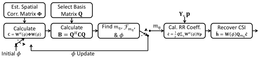
Figure 1: Block diagram of the proposed channel estimation and rank determination procedure.

Remark 5

It is important at this point to mention two known properties governing the mean AoA, AS, spatial correlation, and channel rank. The first property is that the spatial correlation decreases as ULA element spacing and/or the AS $\Delta$ increases [22]. The second property further incorporates the effect of mean AoA $\phi$, stating that the asymptotic normalized channel rank $\lim_{M\rightarrow\infty}\frac{m}{M}=\rho$ is given by [23, Thm. 2]

$$\rho=\min\left\{1,\frac{\xi}{\lambda}|\sin(\phi-\Delta)-\sin(\phi+\Delta)|\right\},$$ (56)

where $-\pi/2<\phi-\Delta<\phi+\Delta<\pi/2$. The above equation indicates that for a fixed $\phi$, $\rho$ increases as $\Delta$ becomes larger and; for a fixed $\Delta$, a $\phi$ that is closer to $0$ leads to a larger $\rho$. In the finite $M$ regime such behaviors are also verified in [24] and in the following section.

VII Numerical Results and Discussion

In this section, we investigate the effects of key system design parameters such as the basis used, modeling order, and channel parameters as SNR (32), channel correlation, AS, and mean AoA on the RR channel estimator performance. Unless otherwise specified, we assume a $100$-element ULA with antenna spacing $0.5\lambda$ and use the standardized SCM channel model [25] with a single cluster that contains $20$ subpaths.

VII-A AoA Alignment, Bases, and Model Order

In Section IV-B2, we have mentioned that the estimator $\hat{\mathbf{h}}_{m}$ and $\hat{\mathbf{h}}^{\prime}_{m}$ differ in that the former attempts to redistribute the average energy of an LPM channel vector having an approximately real-valued correlation matrix in a reduced-dimension subspace while the latter has to deal with one that has complex-valued spatial correlations. We therefore predicted that the LPM based estimator $\hat{\mathbf{h}}_{m}$ performs better than $\hat{\mathbf{h}}^{\prime}_{m}$, the one without the LPM operation, in that the former offers more reduction on rank. Fig. 2 confirms such a prediction; it shows that one needs to find only one index ${m_{\eta}}$ instead of two required by $\hat{\mathbf{h}}^{\prime}_{m}$ which also has a inferior rank reduction capability. Mean AoA estimate is a by-product of $\hat{\mathbf{h}}_{m}$.

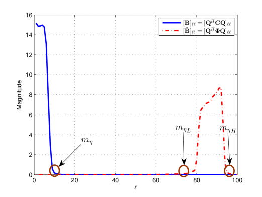
Figure 2: Channel Energy spectra (the diagonal terms of bias matrices) with respect to the DCT basis with (solid curve) and without (dotted curve) mean AoA alignment; $\xi=\lambda/2$, $M=100$ $\mathrm{AS}=7.2^{\circ}$, known mean AoA $\phi=60^{\circ}$.

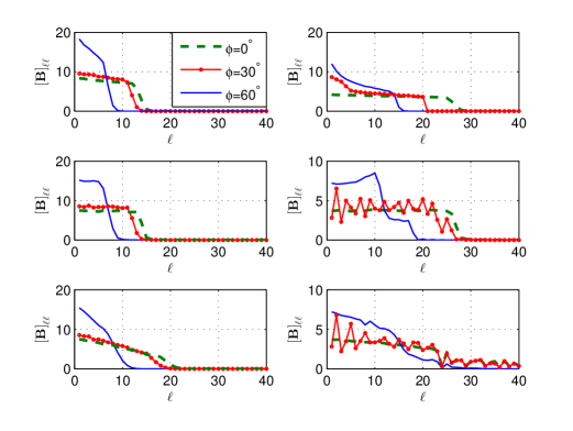
Figure 3: LPM channel energy spectra ($[\mathbf{B}]_{\ell\ell}$) seen by different bases. The left and right columns of sub-figures assume $\mathrm{AS}=7.2^{\circ}$ and $15^{\circ}$, respectively. The top, middle, and bottom rows are the spectra with respect to KLT, DCT, and polynomial bases.

Fig. 3 shows the energy spectra of highly ($\mathrm{AS}=7.2^{\circ}$) and moderately ($\mathrm{AS}=15^{\circ}$) correlated channels with respect to the KLT, DCT, and polynomial bases after LPM operation. For all three bases considered, the channel rank is an increasing function of the AS and a decreasing function of the mean AoA $\phi$. This trend has been predicted in Remark 5. As expected, the KLT basis is indeed the most efficient in that it requires the least modeling order $m$, among the three bases, to characterize the $M$-dimensional channel. The DCT and polynomial bases give similar performance when AS is small but the polynomial basis degrades significantly at $\mathrm{AS}=15^{\circ}$.

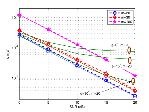
Figure 4: Effect of the modeling order on the MSE performance of the polynomial-based CE $\hat{\mathbf{h}}_{m}$ with known LSFCs; $\mathrm{AS}=7.2^{\circ}$, $\phi=60^{\circ}$. Both theoretical MSE performance with known $\phi$ (solid curves) and simulated counterpart (dashed curves) are shown. Also shown is the theoretical performance as a function of $\phi$ when the modeling order is $m=20$.

Figure 5: Rank selection effect on the DCT-based CE $\hat{\mathbf{h}}_{m}$’s simulated (dashed) and theoretical (solid curves) MSE performance with known LSFCs; $\mathrm{AS}=15^{\circ}$, $\phi=0^{\circ}$. The impact of $\phi$ on a fixed-$m$ estimator is also shown.

The effect of the modeling order on the DCT- and polynomial-based channel estimators’ MSE performance is examined in Figs. 4 and 5 for $(\mathrm{AS},\phi)=(7.2^{\circ},60^{\circ})$ and $(15^{\circ},0^{\circ})$, respectively. When the AS is small ($7.2^{\circ}$), the spatial correlation is relatively high (cf. Remark 5) so we need a small modeling order. Fig. 4 shows that over-modeling the channel (as $m$ increases from $20$ to $100$) in fact degrades the MSE performance. But when $\mathrm{AS}$ increases to $15^{\circ}$, the spatial correlation decreases and the spatial channel roughens, hence a larger $m$ is called for, especially at higher SNR; see Fig. 5. In both figures we also show the MSE performance (solid curves without markers) for some selected mean AoAs. We find that, for a fixed AS and SNR, the optimal modeling order is a decreasing function of $|\phi|$, which is consistent with what Remark 5 and Fig. 3 have predicted: the channel correlation increases with decreasing $|\phi|$.

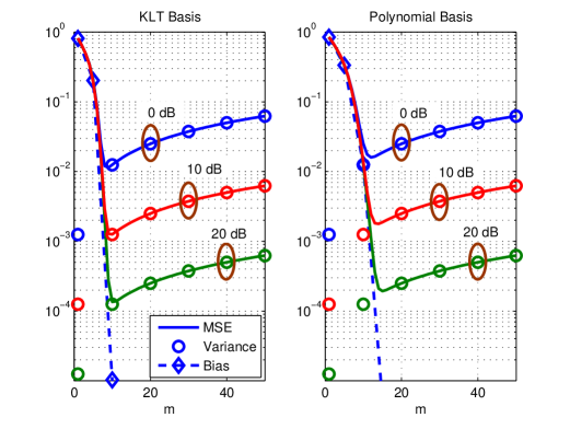
Figure 6: MSE, variance, and bias (all normalized by $M=100$) of the RR channel estimator versus modeling order and ${\alpha}$; $\mathrm{AS}=7.2^{\circ}$, known mean AoA $\phi=60^{\circ}$.

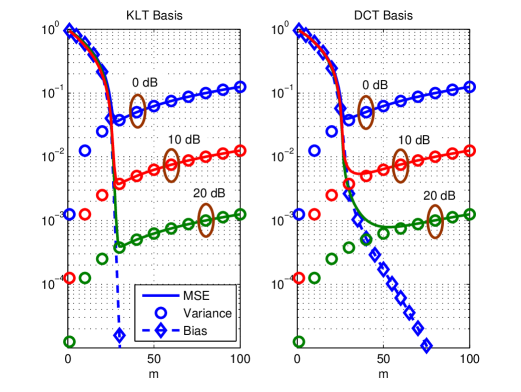
Figure 7: MSE, variance, and bias (all normalized by $M$) behaviors of the RR channel estimator versus $m$ and ${\alpha}$; $\mathrm{AS}=15^{\circ}$, known mean AoA $\phi=0^{\circ}$.

In Figs. 6 and 7, we plot the bias, variance, and MSE with respect to modeling order $m$ of the estimator (13) in a high and moderate spatial correlated channels. The MSE-minimizing modeling order $m^{\star}$, for each scenario corresponding to different bases and SNRs can be found in these two figures. Lemma 4 is numerically verified and the associated $m^{\star}$ and ${m_{\eta}}$ are listed in Tables I and II. When SNR becomes larger, MSE becomes more bias-dominant (cf. Remark 4) and so $\eta$ should be chosen to be closer to $1$. When $\eta$ is so adaptive to SNR, ${m_{\eta}}$ is close to ${m}^{\star}$ and we have near-optimal MSE performance. As expected, the KLT-based estimator requires the smallest modeling order and achieves the best MSE performance.

TABLE I: Modeling orders which minimize the MSE of CEs and bias and those derived from IMOD algorithm for $(\mathrm{AS},\phi)=(7.2^{\circ},60^{\circ})$.

KLT Basis
${\alpha}$	$0$ dB	$10$ dB	$20$ dB
${m}^{\star}$	$9$	$10$	$10$
${m_{\eta}}$ ($\phi$, $\mathbf{\Phi}$ known)	8                      ($\eta=0.99$)	9                      ($\eta=0.999$)	10 ($\eta=0.9999$)
${\hat{m}_{\eta}}$ ($\mathbf{\Phi}$ known)	$8.0$                      ($\eta=0.99$)	$9.0$ ($\eta=0.999$)	$10.0$ ($\eta=0.9999$)
${\hat{m}_{\eta}}$ ($\hat{\mathbf{\Phi}}$, $J=10$)	$10.3$                      ($\eta=0.9$)	$19.7$ ($\eta=0.99$)	$20.3$ ($\eta=0.999$)
Polynomial Basis
${\alpha}$	$0$ dB	$10$ dB	$20$ dB
${m}^{\star}$	$12$	$14$	$15$
${m_{\eta}}$ ($\phi$, $\mathbf{\Phi}$ known)	11                      ($\eta=0.99$)	12 ($\eta=0.999$)	14 ($\eta=0.9999$)
${\hat{m}_{\eta}}$ ($\mathbf{\Phi}$ known)	$13.5$                      ($\eta=0.99$)	$16.1$ ($\eta=0.999$)	$17.4$ ($\eta=0.9999$)
${\hat{m}_{\eta}}$ ($\hat{\mathbf{\Phi}}$, $J=10$)	$9.0$                      ($\eta=0.9$)	$12.0$ ($\eta=0.99$)	$13.6$ ($\eta=0.999$)

TABLE II: Modeling orders which minimize the MSE of CEs and bias and those derived from the IMOD algorithm for $(\mathrm{AS},\phi)=(15^{\circ},0^{\circ})$.

KLT Basis
${\alpha}$	$0$ dB	$10$ dB	$20$ dB
${m}^{\star}$	$28$	$29$	$31$
${m_{\eta}}$ ($\phi$, $\mathbf{\Phi}$ known)	27                      ($\eta=0.99$)	28 ($\eta=0.999$)	30 ($\eta=0.9999$)
${\hat{m}_{\eta}}$ ($\mathbf{\Phi}$ known)	$27.0$                      ($\eta=0.99$)	$28.0$ ($\eta=0.999$)	$30.0$ ($\eta=0.9999$)
${\hat{m}_{\eta}}$ ($\hat{\mathbf{\Phi}}$, $J=10$)	$10.9$                      ($\eta=0.9$)	$20.1$ ($\eta=0.99$)	$21.5$ ($\eta=0.999$)
DCT Basis
${\alpha}$	$0$ dB	$10$ dB	$20$ dB
${m}^{\star}$	$29$	$37$	$53$
${m_{\eta}}$ ($\phi$, $\mathbf{\Phi}$ known)	27                      ($\eta=0.99$)	36 ($\eta=0.999$)	56 ($\eta=0.9999$)
${\hat{m}_{\eta}}$ ($\mathbf{\Phi}$ known)	$28.3$ ($\eta=0.99$)	$37.7$ ($\eta=0.999$)	$59.1$ ($\eta=0.9999$)
${\hat{m}_{\eta}}$ ($\hat{\mathbf{\Phi}}$, $J=10$)	$24.8$                      ($\eta=0.9$)	$28.6$ ($\eta=0.99$)	$37.2$ ($\eta=0.999$)

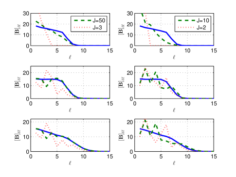
Figure 8: Estimated channel spectra at ${\alpha}=10$ dB; $\mathrm{AS}=7.2^{\circ}$, and $\phi=60^{\circ}$ (known). Estimated LPM spectra in the left column of sub-figures are obtained with $50$ or $3$ samples, whereas $10$ or $2$ in the right. The sub-figures in the top, middle, and bottom rows are the spectra with respect to the KLT, DCT, and polynomial bases. The blue solid curves correspond to the results of the true $\mathbf{\Phi}$.

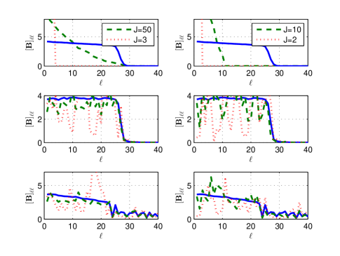
Figure 9: Estimated and true LPM channel spectra at ${\alpha}=10$ dB; $\mathrm{AS}=15^{\circ}$, and $\phi=0^{\circ}$ (known). Estimated spectra in the left sub-figures are obtained with $50$ or $3$ samples, whereas $10$ or $2$ samples are used elsewhere. The sub-figures in the top, middle, and bottom rows are the spectra with respect to the KLT, DCT, and polynomial bases. The blue solid curves are associated with the true $\mathbf{\Phi}$.

VII-B Spatial Correlation, Receive Beamforming, and Multi-cluster Channels

Also shown in Table I and II are the average ${\hat{m}_{\eta}}$’s obtained via the IMOD algorithm, which usually converges in just a few (no more than five) iterations. A more realistic scenario when $\mathbf{\Phi}$ is estimated by substituting $\mathbf{\Psi}$ in (54) with (55) using $J=10$ periods samples is considered there as well. Figs. 8 and 9 show the corresponding estimated channel spectra. As $\hat{\boldsymbol{\Psi}}$ is obtained by averaging $J$ outer product matrices and has a rank less than or equal to $J$, we cannot find a proper estimate of ${m_{\eta}}$ for KLT basis when the true dominant rank exceeds the number of sample periods. This is a shortcoming of the KLT approach when the associated correlation matrix has to be estimated by averaging small time-domain samples. This sample-deficient problem exists for other similar rank determination methods [20, 21] but is of much less concern for the predetermined basis approach we have adopted.

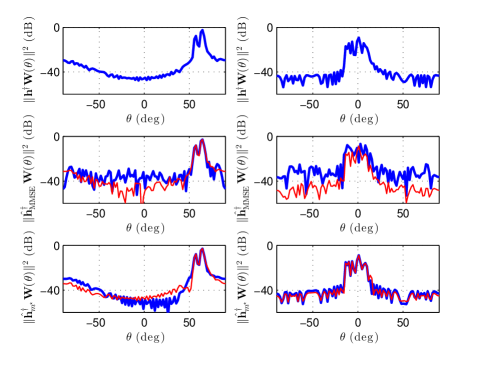
Figure 10: Beam patterns implied by the proposed RR channel estimator for two known mean AoAs at ${\alpha}=0$ dB. The left and right sub-figures assume $(\mathrm{AS},\phi)=(7.2^{\circ},60^{\circ})$ and $(15^{\circ},0^{\circ})$ and those in the top, middle, and bottom rows are generated by the true channel vector, MMSE [4], and RR estimate (13), respectively. Red and blue curves represents respectively the results with perfect $\mathbf{\Phi}$ or its estimated counterpart using $J=10$ samples.

We now verify the effectiveness of our RR channel estimator from the receiver’s viewpoint which is similar to but slightly different from what was discussed in Remark 3. We notice that a maximum-ratio combining (MRC) receiver would first multiply a received vector ${\mathbf{y}}$ by $\hat{\mathbf{h}}^{\dagger}$, the pseudoinverse of the channel estimate $\hat{\mathbf{h}}$, before making hard or soft symbol decisions. This operation is equivalent to receive beamforming. A receive beamformer which acts as a spatial filter should conceivably match the incoming signal beam pattern: it should point toward the mean AoA with a (main) beamwidth approximately equal to the 2-sided AS so that the dominant part of the signal carried by the channel vector is filtered with minimum distortion while noise or interference from other directions are suppressed. This prediction is confirmed by Fig. 10; see (III-B).

Although the MMSE channel estimator [4]

$$\hat{\mathbf{h}}=\mathbf{\Phi}\left(\|\mathbf{p}\|^{2}\mathbf{\Phi}+\mathbf{I}_{M}\right)^{-1}\left(\mathbf{p}^{T}\otimes\mathbf{I}_{M}\right)\mathrm{vec}(\mathbf{Y})$$

yields performance similar to the RR estimators when ${\bf\Phi}$ is perfectly known, it is sensitive to the correlation matrix estimation error. In contrast, our estimator is more robust as it does not need complete and accurate information about ${\bf\Phi}$, all it needs is the dominant rank of the channel spectrum and the associated dominant support.

Finally, to demonstrate that our channel estimator is applicable to multi-cluster channels, we show two examples in Fig. 11. In the upper sub-figure, the two clusters are separable both spatially, i.e., $[{\phi}_{1}-\Delta_{1},{\phi}_{1}+\Delta_{1}]=[52.8^{\circ},67.2^{\circ}]$ and $[{\phi}_{2}-\Delta_{2},{\phi}_{2}+\Delta_{2}]=[0^{\circ},30^{\circ}]$, and in the DFT domain. As a result, the dominant support consists of two disjoint sets, $\mathcal{F}_{m}=[1,{m_{\eta}}_{1}]\cup[{m_{\eta}}_{2},{m_{\eta}}_{3}]$, so the multi-cluster channel can be estimated via (4) with $\mathbf{Q}_{m}\stackrel{{\scriptstyle def}}{{=}}[{\mathbf{q}}_{\ell}]_{\ell\in\mathcal{F}_{m}}$. In the lower sub-figure we consider a channel with two overlapped clusters which are inseparable. By treating this channel as a single-cluster channel, we still can apply our scheme with dominant support $\mathcal{F}_{m}=[{m_{\eta}}_{4},{m_{\eta}}_{5}]$ to obtain a CE.

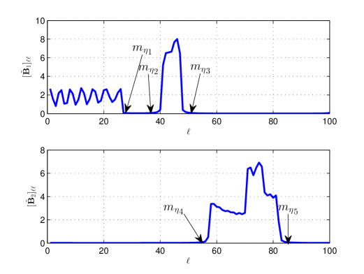
Figure 11: Channel energy spectra of two $2$-cluster channels with respect to the DFT basis. (Upper part) $(\Delta_{1},{\phi}_{1})=(7.2^{\circ},60^{\circ})$ and $(\Delta_{2},{\phi}_{2})=(15^{\circ},15^{\circ})$; (Bottom) $(\Delta_{1},{\phi}_{1})=(7.2^{\circ},-30^{\circ})$ and $(\Delta_{2},{\phi}_{2})=(15^{\circ},-45^{\circ})$.

VIII Conclusion

In this paper, we extend a model-based RR channel estimator for use in spatially-correlated massive MIMO systems. The two proposed estimators’ rank-reduction nature and looser spatial correlation information requirement result in performance improvement over conventional LS and MMSE estimators and lower complexity in post-channel-estimation signal processing. One of the estimator–the LPM-aided one–obtain a mean AoA estimate as a by-product. The LPM operation is shown to offer another benefit of further rank reduction when the DCT basis is employed, resulting in near-optimal energy compaction and performance.

We analyze the impacts of and interrelations among the critical design issues such as basis selection and rank determination and other system/channel parameters’ (e.g., SNR, spatial correlation, mean AoA and AS) on the estimators’ MSE performance. The analytic relation between the channel’s energy spectrum and the estimator’s MSE enable us to develop efficient rank and/or mean AoA estimation methods. Viewing the channel estimation problem from different perspectives helps casting new insights into the problem of concern. Although we focus our discussion on single-cluster channels, we briefly demonstrate the feasibility of extending our approach to more general multi-cluster channels.

Appendix Appendix A Proof of Lemma 2

In the following, we derive the variance and bias terms of the MSE of $\hat{\mathbf{h}}_{m}$ (5). Those of $\hat{\mathbf{h}}^{\prime}_{m}$ for the regular model (4) can be similarly obtained. We start with

$$\mathrm{Var}\{\hat{\mathbf{h}}_{m}\} = \mathbb{E}\left\{\left\|\hat{\mathbf{h}}_{m}-\mathbb{E}\{\hat{\mathbf{h}}\}\right\|^{2}\right\}~{}~{}~{}~{}$$ (A.1)

$$= \frac{1}{\gamma^{2}}\mathbf{p}^{H}\mathbb{E}\left\{\mathbf{N}^{H}\mathbf{W}(\hat{\phi})\mathbf{Q}_{m}\mathbf{Q}_{m}^{H}\mathbf{W}^{H}(\hat{\phi})\mathbf{N}\right\}\mathbf{p}$$

$$= \frac{1}{\gamma^{2}}\mathbf{p}^{H}\mathrm{tr}\left(\mathbf{W}(\hat{\phi})\mathbf{Q}_{m}\mathbf{Q}_{m}^{H}\mathbf{W}^{H}(\hat{\phi})\right)\mathbf{I}_{T}\mathbf{p}$$

$${=} \frac{1}{\gamma^{2}}\mathbf{p}^{H}(m)\mathbf{p}=\frac{m}{\beta\|\mathbf{p}\|^{2}}$$

where we have invoked the relation

$$\mathbb{E}\left\{\mathbf{N}^{H}\mathbf{X}\mathbf{N}\right\} = \sum_{i=1}^{M}\sum_{j=1}^{M}x_{ij}\mathbb{E}\left\{\mathbf{n}_{i}\mathbf{n}_{j}^{H}\right\}$$ (A.2)

$$= \sum_{i=1}^{M}x_{ii}\mathbb{E}\left\{\mathbf{n}_{i}\mathbf{n}_{i}^{H}\right\}=\mathrm{tr}(\mathbf{X})\mathbf{I}_{T}~{}~{}~{}$$

with white noise $\mathbf{N}=\left[\mathbf{n}_{1},\cdots,\mathbf{n}_{M}\right]^{H}$ for any square matrix $\mathbf{X}=[x_{ij}]$. For the bias term, we have

$$b(\hat{\mathbf{h}}_{m}) = \mathbb{E}\left\{\left\|\mathbb{E}\{\hat{\mathbf{h}}_{m}\}-\mathbf{h}\right\|^{2}\right\}$$

$$= \mathbb{E}\left\{\mathbf{h}^{H}\left(\mathbf{W}(\hat{\phi})\mathbf{Q}_{m}\mathbf{Q}_{m}^{H}\mathbf{W}^{H}(\hat{\phi})-\mathbf{I}_{M}\right)^{2}\mathbf{h}\right\}$$

$$= \mathrm{tr}\left(\left(\mathbf{W}(\hat{\phi})\mathbf{Q}_{m}\mathbf{Q}_{m}^{H}\mathbf{W}^{H}(\hat{\phi})-\mathbf{I}_{M}\right)^{2}\mathbf{\Phi}\right).\vspace{-1em}$$

$$\hskip 16.99998pt\underbrace{\hskip 132.00017pt}_{\stackrel{{\scriptstyle def}}{{=}}\mathbf{A}_{1}}$$

Since

$$\mathbf{Q}_{m}\mathbf{Q}_{m}^{H} = \mathbf{Q}(\mathbf{I}_{M}-\mathbf{D}_{m})\mathbf{Q}^{H}$$ (A.3)

where $\mathbf{D}_{m}$ is an idempotent matrix, i.e., $\mathbf{D}_{m}^{2}=\mathbf{D}_{m}$, we have $\mathbf{A}_{1}=\mathbf{W}(\hat{\phi})\mathbf{Q}\mathbf{D}_{m}\mathbf{Q}^{H}\mathbf{W}^{H}(\hat{\phi})$ and

$$b(\hat{\mathbf{h}}_{m}) = \mathrm{tr}\left(\mathbf{W}(\hat{\phi})\mathbf{Q}\mathbf{D}_{m}\mathbf{Q}^{H}\mathbf{W}^{H}(\hat{\phi})\mathbf{\Phi}\right)$$ (A.4)

$$= \mathrm{tr}\left(\mathbf{D}_{m}\mathbf{Q}^{H}\mathbf{W}^{H}(\hat{\phi})\mathbf{\Phi}\mathbf{W}(\hat{\phi})\mathbf{Q}\right)$$

$$= \mathrm{tr}\left(\mathbf{D}_{m}\hat{\mathbf{B}}\right)=\sum_{\mathcal{F}^{c}_{m}}[\hat{\mathbf{B}}]_{\ell\ell}=\langle\mathbf{D}_{m},\hat{\mathbf{B}}\rangle_{F},~{}~{}~{}~{}$$

the Frobenius product of $\mathbf{D}_{m}$ and $\hat{\mathbf{B}}$.

References

- [1] F. Rusek, D. Persson, B. K. Lau, E. G. Larsson, T. L. Marzetta, O. Edfors, and F. Tufvesson, “Scaling up MIMO: opportunities and challenges with very large arrays,” IEEE Signal Proces. Mag., vol. 30, no. 1, pp. 40–60, Jan. 2013.
- [2] S. Payami and F. Tufvesson, “Channel measurements and analysis for very large array systems at 2.6 GHz,” in Proc. EuCAP 2012, Prague, Czech, Mar. 2012.
- [3] M. Biguesh and A. B. Gershman, “Training-based MIMO channel estimation: a study of estimator tradeoffs and optimal training signals,” IEEE Trans. Signal Process., vol. 54, no. 3, pp. 884–893, Mar. 2006.
- [4] H. Yin, D. Gesbert, M. Filippou, and Y. Liu, “A coordinated approach to channel estimation in large-scale multiple-antenna systems,” IEEE J. Sel. Areas Commun., vol. 31, no. 2, pp. 264–273, Feb. 2013.
- [5] D. C. Araùjo, A. L. F. de Almeida, J. Axnäs, and J. C. M. Mota, “Channel estimation for millimeter-wave very-large MIMO systems,” in Proc. EUSIPCO 2014, Lisbon, Portugal, Sep. 2014.
- [6] C.-K. Wen, S. Jin, K.-K. Wong, J.-C. Chen, and P. Ting, “Channel estimation for massive MIMO using Gaussian-mixture Bayesian learning,” IEEE Trans. Wireless Commun., vol. 14, no. 3, pp. 1356–1368, Mar. 2015.
- [7] Y.-C. Chen and Y. T. Su, “MIMO channel estimation in correlated fading environments,” IEEE Trans. Commun., vol. 9, no. 3, pp. 1108–1119, Mar. 2010.
- [8] K.-F. Chen, Y.-C. Liu, and Y. T. Su, “On composite channel estimation in wireless massive MIMO systems,” in Proc. IEEE GLOBECOM Workshops 2013, pp. 135–139, Atlanta, GA, Dec. 2013.
- [9] Q. Zhang, X. Zhu, Y. Yang, P. Shang, and J. Liu, “Efficient transform-domain channel estimation technique for large-scale multiple antenna systems,” in Proc. IEEE PIMRC 2014, pp. 448–452, Washington, D.C., Sep. 2014.
- [10] P. Zhang, L. Gan, S. Sun, and C. Ling, “Atomic norm denoising-based channel estimation for massive multiuser MIMO systems,” in Proc. IEEE ICC 2015, pp. 4564–4569, London, UK, Jun. 2015.
- [11] V. Kristem, S. Sangodoyin, C. U. Bas, M. Käske, J. Lee, C. Schneider, G. Sommerkorn, J. Zhang, R. Thomä, and A. F. Molisch, “3D MIMO outdoor to indoor macro/micro-cellular channel measurements and modeling,” in Proc. GLOBECOM 2015, San Diego, CA, Dec. 2015.
- [12] D.-S. Shiu, G. J. Foschini, M. J. Gans, and J. M. Kahn, “Fading correlation and its effect on the capacity of multielementantenna systems,” IEEE Trans. Commun., vol. 48, no. 3, pp. 502–513, Mar. 2000.
- [13] A. M. Sayeed, “Deconstructing multiantenna fading channels,” IEEE Trans. Signal Process., vol. 50, no. 10, pp. 2563–2579, Oct. 2002.
- [14] W. Weichselberger, M. Herdin, H. Özcelik, and E. Bonek, “A stochastic MIMO channel model with joint correlation of both link ends,” IEEE Trans. Wireless Commun., vol. 5, no. 1, pp. 90–100, Jan. 2006.
- [15] C.-X. Wang, X. Hong, H. Wu and W. Xu, “Spatial-temporal correlation properties of the 3GPP spatial channel model and the Kronecker MIMO channel model,” EURASIP J. Wireless Commun. and Netw., 2007.
- [16] K. R. Rao and P. C. Yip, The Transform and Data Compression Handbook, CRC Press, Inc., 2000.
- [17] P. R. Haddad and A. N. Akansu, Multiresolution Signal Decomposition, Second Edition: Transforms, Subbands, and Wavelets, Academic Press, 2000.
- [18] N. Ahmed, T. Natarajan, and K. R. Rao, “Discrete cosine transform,” IEEE Trans. Comput., vol. C-23, no. 1, pp. 90–93, Jan. 1974.
- [19] A. V. Oppenheim and R. W. Schafer, Discrete-Time Signal Processing: Third Edition, Pearson, 2010.
- [20] C. J. Zarowski, “The MDL criterion for rank determination via effective singular values,” IEEE Trans. Signal Process., vol. 46, no. 6, pp. 1741–1744, Jun 1998.
- [21] J. J. Blanz, “Method and apparatus for reduced rank channel estimation in a communications system,” U.S. Patent 6,907,270, issued June 14, 2005.
- [22] J. A. Tsai, R. M. Buehrer, and B. D. Woerner, “The impact of AOA energy distribution on the spatial fading correlation of linear antenna array,” in Proc. IEEE VTC 2002, vol. 2, pp. 933–937, Birmingham, AL, May 2002.
- [23] A. Adhikary, J. Nam, J.-Y. Ahn, and G. Caire, “Joint spatial division and multiplexing–the large-scale array regime,” IEEE Trans. Inf. Theory, vol. 59, no. 10, Oct. 2013.
- [24] J. Fuhl, A. F. Molisch, and E. Bonek, “Unified channel model for mobile radio systems with smart antennas,” Proc. IEE–Radar, Sonar Navig., vol. 145, no. 1, pp. 32–41, Feb. 1998.
- [25] “Spatial channel model for multiple input multiple output (MIMO) simulations,” 3GPP TR 25.996 V11.0.0, Sep. 2012. [Online]. Available: http://www.3gpp.org/ftp/Specs/html-info/25996.htm.