Dissecting cross-impact on stock markets: An empirical analysis

Abstract

The vast majority of market impact studies assess each product individually, and the interactions between the different order flows are disregarded. This strong approximation may lead to an underestimation of trading costs and possible contagion effects. Transactions in fact mediate a significant part of the correlation between different instruments. In turn, liquidity shares the sectorial structure of market correlations, which can be encoded as a set of eigenvalues and eigenvectors. We introduce a multivariate linear propagator model that successfully describes such a structure, and accounts for a significant fraction of the covariance of stock returns. We dissect the various dynamical mechanisms that contribute to the joint dynamics of assets. We also define two simplified models with substantially less parameters in order to reduce overfitting, and show that they have superior out-of-sample performance.

1 Introduction

Price impact in financial markets – the effect of transactions on the observed market price – is of both scientific and practical relevance [1]. A long series of studies has concentrated on its various aspects in the past decades [2, 3, 4, 5, 6, 7, 8, 9]. The metrics used in this body of work are usually calculated individually on each product, and possibly averaged across them afterwards. The interactions between their order flows are typically disregarded. This is a very strong approximation, given that a financial instrument is rarely traded on its own. Most investors construct diversified portfolios by buying and selling tens or even hundreds of assets at the same time. Some of these might be similar, or even almost equivalent to each other (companies in the same industrial sector, dual-listed shares, etc.). In these cases it is immediately clear that to treat each of them separately is not justified, and often an underestimation of impact costs. Intuition tells us that in two related products the order flow of one of them may reveal information, or communicate excess supply/demand regarding the other. How important are such effects, both qualitatively and quantitatively?

The “self-impact” of a product’s order flow on its own price, as studied in the literature, is an important component of price dynamics. In comparison, is “cross-impact” a detectable effect? If it is, is it strong enough to significantly contribute to cross-correlations between stocks? This question was already raised in the seminal work of Hasbrouck and Seppi [10]. It is particularly interesting, because in spite of the importance of cross-correlations in risk management, their microstructural origin is not clear. Many partial, competing explanations exist, for a review of recent economics literature on the subject see in Ref. [11]. When choosing their quotes, liquidity providers use correlation models calibrated from real data. It would thus be a circular argument to fully ascribe such correlations emerge to market makers’ quote adjustments. A dynamical explanation is more plausible. When two stocks get out of line relative to one another, liquidity takers may also act on such a mispricing. As they consume liquidity, market makers adjust their pricing to avoid building up a large inventory: this is price impact. As the relative price reaches a (temporary) market consensus order flows become balanced. Several structural, equilibrium theories exist with such dynamics, but the underlying models often have many parameters which cannot be directly fitted to data. Only the qualitative predictions can be observed, which are nevertheless very important for practical purposes [12].

In this manuscript we argue in favor of such a dynamical picture, where transactions mediate a significant part of the interaction between different instruments, and price impact is an integral part of price formation. We will demonstrate quantitatively that correlations and liquidity are intertwined. Refs. [13, 14] revisit the evidence for cross-impact by analyzing the cross-correlation structure of price changes and order flows. Our study complements such a perspective by focusing on the underlying interactions rather than on correlations. Based on a variant of the well-known propagator technique [6], calibrated on anonymous data, we will show that liquidity displays a sectorial structure related to the one of market correlations, that we will be able to describe through decomposition in eigenvalues and eigenvectors. This is in the spirit of the principal component analysis approach advocated in Ref. [10], and the analysis of Ref. [12] from an econometric point of view.

For the sake of simplicity we will use here the language of stocks, and we will in fact limit our datasets to these. However, the techniques introduced below can be applied to many other markets. Moreover, note that we focus here on the impact of the aggregated order flow, rather than the one of a meta-order (a sequence of trades in the same direction submitted by the same actor). Even though the propagator formalism that we employ is known to predict inaccurately the impact of a meta-order, it still provides qualitatively reliable estimates of market impact (see Section 5 of Ref. [15]). Thus, we believe that the cross-interaction network that we find should generalize to the meta-order case as well, at least to a good approximation.

The paper is structured as follows. Section 2 introduces basic notations and our dataset. Section 3 defines a few fundamental quantities related to returns and price impact, and summarizes that main stylized facts that we observe. Section 4 provides a non-parametric multivariate propagator model, which is then fitted to the data. Section 5 analyzes simpler, lower-dimensional models that can more efficiently capture the structure of cross-impact; and compares their in-sample and out-of-sample performance. Finally, Section 6 concludes.

2 Data and notations

We conduct our empirical analysis on a pool of $N=275$ US stocks as representative as possible in terms of liquidity, market capitalisation and tick size. The large number of assets and their diversity ensures strong statistical significance, and allows us to investigate the scaling of our results when the number of products becomes large. The data consists of five-minute binned trades and quotes information from January 2012 to December 2012, extracted from the primary market of each stock (NASDAQ or NYSE). Furthermore, we only focus on the continuous trading session, removing systematically the first hour after the open and the last 30 minutes before the close. In this way we avoid artifacts arising from the particularities of trading activity in these periods. Out-of-sample tests will be carried out on an equivalent dataset from 2013.

For each five-minute window whose end point is $t$ and for each asset $i$, we compute the log-return $x^{{i}}_{t}=X^{{i}}_{t}-X^{{i}}_{t-1}$, where $X^{{i}}_{t}=\log p^{{i}}_{t}$ and where $p^{{i}}_{t}$ denotes the price of stock $i$ at time $t$. In addition, we compute the trade imbalance $\varepsilon^{{i}}_{t}=n^{i,\mathrm{buy}}_{t}-n^{i,\mathrm{sell}}_{t}$, where $n^{i,\mathrm{buy/sell}}_{t}$ denotes respectively the number of buyer- and seller-initiated market orders of stock $i$ in bin $t$. We choose this proxy for volume imbalance because the strong fluctuations in the size of the trades are only moderately compensated by the information that they provide [4, 6].

We normalise $x^{i}_{t}$ and $\varepsilon^{i}_{t}$ by their standard deviation computed over the entire trading period. As a result, both time series display zero mean and unit variance. This choice of normalisation has the benefit of making the problem extensive in the following sense: For any linear model that one infers, (such as the one presented in Section 4.1), the results obtained for a larger bin size (say, one hour) can always be recovered from the results obtained at a finer scale. Moreover, extensivity allows the predictions of the model not to depend on the estimation of the local normalization. One does not need to build estimators for volatility and volume in the next five-minutes bin in order to exploit these results. This would not have been the case had we used a local normalization for the fluctuations of the returns and the volumes. Still, we have checked that the choice of a local normalization, while spoiling extensivity, yields qualitatively similar results.

Also note that we have chosen to use real time to measure $t$ as opposed to counting it on a trade-by-trade basis. This is because in the regime of large $N$ that we consider, there would be too many trades, and our dataset would become unmanageable [14, 13]. Finally, the choice of a five-minute bin size allows us to abstract away from microstructure effects which are not the subject of the present mesoscopic study. All along this manuscript time shall be seen as dimensionless, five minutes being the time unit.

3 Market impact and price fluctuations

In this section, we define the multivariate correlation functions relevant to the problem at hand, and investigate their relations.

3.1 The correlation structure of returns

The covariance matrix of returns is one of the central objects in quantitative finance, and is of paramount importance in a number of applications such as portfolio construction and risk management [16, 17]. Let us recall first some of its most prominent properties.

We denote by $\Sigma^{ij}_{\tau}$ the return covariance of contracts $i$ and $j$ at scale $\tau$, defined as

$$\Sigma^{ij}_{\tau}=\mathbb{E}[(X^{{i}}_{t+\tau}-X^{{i}}_{t})(X^{j}_{t+\tau}-X^{j}_{t})]$$ (1)

Figure 1(a) displays a plot of the mean diagonal $\Sigma^{\mathrm{diag}}_{\tau}=N^{-1}\sum_{i}\Sigma^{ii}_{\tau}$ and off-diagonal $\Sigma^{\mathrm{off}}_{\tau}=(N^{2}-N)^{-1}\sum_{i\neq j}\Sigma^{ij}_{\tau}$ return covariances rescaled by $\tau$. As one can see, the diagonal terms of the return covariance matrix are on average a factor $\sim 5$ larger than the off-diagonal ones. Microstructural effects are almost absent in $\Sigma^{ij}_{\tau}$ even at $\tau=1$: we only observe a weak decrease of the variance at short lags in the signature plot, and the ratio between covariance and variance – that determines the so-called Epps effect [18, 19] – is almost flat in $\tau$. This is consistent with the absence of statistical arbitrage price, because the time scale for these arbitrage effects is nowadays expected to be well below the five-minute time scale [20, 21, 22]. Finally, one can define the customary return correlation matrix as $\Sigma^{ij}_{\tau}(\Sigma^{ii}_{\tau}\Sigma^{jj}_{\tau})^{-1/2}$.

Figure 2(a) displays a representation of $\Sigma^{ij}_{\tau}$ at $\tau=1$ from which we subtracted its mean ($\approx 0.21$) for better readability, and in which the contracts have been sorted by industrial sector, as indicated by the labels. As one can see, $\Sigma^{ij}_{\tau}$ displays a strong sectorial structure, in line with previous studies [23, 24, 25]. The behaviour of the covariance matrix is best understood in its eigenbasis. Indeed, $\Sigma^{ij}_{\tau}$ is a real symmetric matrix, so it be diagonalised as

$$\Sigma^{ij}_{\tau}=\sum_{a}O^{ia}_{\tau}\Lambda^{a}_{\tau}O^{ja}_{\tau}.$$ (2)

$O^{ia}_{\tau}$ is an orthogonal matrix, its columns correspond to the eigenvectors of $\Sigma^{ij}_{\tau}$, and $\Lambda^{a}_{\tau}$ is a vector made of the corresponding eigenvalues. Figure 2(b) displays the histogram of the eigenvalues $\Lambda^{a}_{\tau}$ at $\tau=1$. We have assessed their stability by verifying that $\Lambda^{a}_{\tau}\propto\tau$, as it was the case for the average quantities displayed in Fig. 1(a). Interestingly, we find the eigenvectors $O^{ia}$ to be stable in time, indicating that the directional structure of the market is consistent across scales ranging from some minutes to one day, while its associated fluctuations increase linearly. The value of the largest eigenvalue $\Lambda^{0}_{1}\approx 62$, indicates that $\Lambda^{0}_{1}/N\approx 23\%$ of the total variance of the system can be explained by this mode, in good agreement with Ref. [10]. Often referred to as the market mode, it corresponds to a collective – and rather homogeneous – mode, as can be seen on Fig. 2(c). The next few modes after the market mode, individually, explain a considerably smaller part of the variance. Their structure supports an economic interpretation in terms of industrial sectors (see Fig. 2(c) and Ref. [23]). The subsequent modes fall into a noise band that is roughly described by a Marčenko-Pastur distribution [27, 28] (see red curve on Fig. 2(b)), due to the fact that the number of stocks is of the same order of magnitude as the number of observations, making it impossible to obtain a statistically accurate estimation of all the modes.

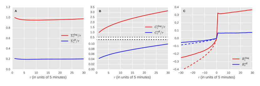
Figure 1: Plots of average diagonal and off-diagonal (a) returns covariance (see Eq. (1)), (b) sign covariance (see Eq. (4)), and (c) response function (see Eq. (5)). The dashed lines for the response indicate the prediction of the model at negative lags.

3.2 The correlation structure of the trade signs

In order to investigate the relation between returns and trade sign imbalance, it is natural to define a covariance matrix for the signs, and to compare its structure with the one built out of the returns. Accordingly, we define the lagged covariance of signs as

$$c^{ij}_{\tau} = \mathbb{E}[\varepsilon^{{i}}_{t+\tau}\varepsilon^{j}_{t}]\ .$$ (3)

Its behaviour is radically different from that of returns. While returns are uncorrelated ($\Sigma^{ij}_{\tau}\sim\tau$ after a few trades) compatible with statistical efficiency of prices, signs are well known to be long-range correlated, as $c^{ij}_{\tau}\sim\tau^{-\gamma}$ with $\gamma\sim 0.5$ (see Appendix). This result stems from the fact that in limit order markets investors split their trading decisions into smaller pieces in order to avoid excessive costs, because instantaneously available liquidity at the best quotes is small [7], much smaller than the daily volume. This yields the famous anomalous response puzzle [6]: Prices diffusive despite being driven by trades which themselves are superdiffusive.

A well-known solution to this problem is that of the linear propagator model (or, equivalently, the surprise model), postulating that trades in the most probable direction impact the price less than those in the unexpected one [6, 7, 29, 1]. While this model has been thoroughly explored in one dimension (with extensions to multi-order types, [8, 30, 31]), its richer multi-dimensional counterpart has not been fully considered yet. A multivariate framework allows to precisely formulate a number of questions that are central to our study, and that cannot be addressed in a one-dimensional setting. What is the role of the trade sign process in shaping the cross-sectional structure of the return correlations? Is there such a thing as a market mode for signs (our proxy for liquidity)? Are there liquidity sectors?

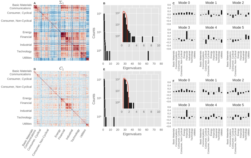
Figure 2: (a) Plot of the returns covariance matrix $\Sigma^{ij}_{\tau}$ at lag $\tau=1$. (b) Histogram of eigenvalues of $\Sigma^{ij}_{1}$. (c) Composition of the eigenvectors (weights per sector). (d-f) Same plots for the sign covariance matrix $C^{ij}_{\tau}$.

In order to push this parallel further, it is useful to define the equal-time covariance $C^{ij}_{\tau}$ of the cumulated trade sign process, which is analogous to $\Sigma^{ij}_{\tau}$, defined as

$$C^{ij}_{\tau}=\mathbb{E}[(\mathcal{E}^{{i}}_{t+\tau}-\mathcal{E}^{{i}}_{t})(\mathcal{E}^{j}_{t+\tau}-\mathcal{E}^{j}_{t})]\ ,$$ (4)

where the $\varepsilon^{i}_{t}$ are the analogue of the “returns” for $\mathcal{E}^{i}_{t}$: $\varepsilon^{i}_{t}=\mathcal{E}^{i}_{t}-\mathcal{E}^{i}_{t-1}$. Figure 1(b) displays a plot of the mean diagonal $C^{\mathrm{diag}}_{\tau}$ and off-diagonal $C^{\mathrm{off}}_{\tau}$ sign covariances rescaled by $\tau$. Similarly to $\Sigma^{ii}_{\tau}$, the diagonal terms are on average larger than the off-diagonal ones, only this time by a factor $\sim 30$. After a short sublinear regime, the results show superlinear time dependence at large $t$, consistent with the long-range correlation of signs for a single asset. Figure 2 shows that, in contrast with the covariance of prices, the covariance of signs displays no or very weak sectorial structure. Although the first mode of the sign covariance also corresponds to a market mode (delocalized and rather homogeneous), it is weaker. Additionally, one has a small number of “sectorial” modes out of the noise band [32], that even in this case are coherent in time, showing a time-overlap close to 1. Despite this, only the market mode is aligned with the market mode of returns. All the other modes show surprisingly small overlap with their return counterparts (see Fig. 7(b) for a quantitative discussion on the fraction of common modes).

3.3 Price response

Do trades shape the return covariance matrix? Or does it result from other mechanisms such such as quote revisions, that do not involve trading volume? In order to address such questions, one needs to look into yet another quantity, the market response $R^{ij}_{\tau}$ defined as:

$$R^{ij}_{\tau}=\mathbb{E}[(X^{{i}}_{t+\tau}-X^{{i}}_{t})\varepsilon^{j}_{t}]\ .$$ (5)

This measures the average price change of contract $i$ at time $t+\tau$, after experiencing a sign imbalance $\varepsilon^{j}_{t}$ in contract $j$ at time $t$. Figure 1(b) displays a plot of the mean diagonal $R^{\mathrm{diag}}_{\tau}$ and off-diagonal $R^{\mathrm{off}}_{\tau}$ responses. The diagonal terms are on average larger than the off-diagonal ones by a factor $\sim 5$. This is consistent with the ratio of the corresponding diagonal/off-diagonal factors for the price and sign covariances, and with the results of Refs. [13, 14]. The response at positive times is roughly constant, consistently with the hypothesis of a statistically efficient price. In other words, the current sign does not predict future returns. The behavior at negative lag indicates that the current return allows some prediction of the sign imbalance, an effect that has been extensively investigated in Refs. [31, 33]. It is worth mentioning that, other than the expected amplitude difference, the off-diagonal response shows the same temporal behaviour than its diagonal counterpart.

4 A simple model for cross-impact

In this section, we present and analyse the implications of the multivariate propagator model, which shall allow us to explain within a coherent framework the stylised facts discussed above.

4.1 The multivariate propagator model

As we shall see the simplest linear model $(i)$ describing the cross-sectional structure of covariance matrices, $(ii)$ accounting for their dynamical structure, and $(iii)$ assuming future signs are weakly affected by recent past returns, is the multivariate propagator model:

$$X^{i}_{t} = {X^{i}_{0}+\sum_{j}\sum_{t^{\prime}=1}^{t}}G^{ij}_{t-t^{\prime}}\varepsilon^{j}_{t^{\prime}}+W^{{i}}_{t}\ .$$ (6)

This expresses the price variations of contract $i$ as a linear regression on the past sign imbalances of all assets $j$. The matrix $G^{ij}_{\tau}$ is customarily called the propagator, as it describes the effect of the trade sign imbalance of contract $j$ at time $t$ on the price of contract $i$ at time $t+\tau$. The quantities $W^{{i}}_{t}$ are defined by $w^{{i}}_{t}=W^{{i}}_{t}-W^{i}_{t-1}$, where the $w^{{i}}_{t}$ are i.i.d. idiosyncratic noises with zero mean and covariance matrix given by

$$\mathbb{E}[w^{{i}}_{t}w^{j}_{t^{\prime}}]=\sigma_{W}^{{ij}}\delta_{t-t^{\prime}}\,,$$ (7)

so that the covariance of the process $W^{{i}}_{t}$ is linear in time, and is given by

$$\Sigma^{ij}_{W,\tau} = \mathbb{E}[(W^{{i}}_{t+\tau}-W^{{i}}_{t})(W^{j}_{t+\tau}-W^{j}_{t})]=\sigma_{W}^{{ij}}\tau\ .$$ (8)

Since we consider a setting in which $\varepsilon_{t}$ is a stationary process, and both $G_{\tau}$ and the correlations of $\varepsilon_{t}$ decay to zero at large lags, it’s straightforward to check that the model defined by (6) converges to a stationary state at large times. Accordingly, in the main text will always refer to the value of the observables $C$, $\Sigma$ and $R$ computed under the stationary measure of the process $\mathbb{E}[\cdots]$. In the calibration of the process we will also assume stationarity to hold, by imposing time-translational invariance for the correlations of $\varepsilon_{t}$ (see Appendix).

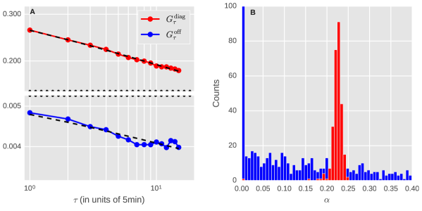
Figure 3: (a) Plot of the mean diagonal and off-diagonal propagators. (b) Corresponding histogram of fitted slopes $\beta$, as given by Eq. (9).

We have fitted the propagator matrix $G^{ij}_{\tau}$ from data. Figure 3(a) displays a plot of the mean diagonal $G^{\mathrm{diag}}_{\tau}$ and off-diagonal $G^{\mathrm{off}}_{\tau}$ propagators that we have obtained under a non-parametric inversion of the model. [See also Section 5 for a comparison of the different inversion techniques that we have adopted.] The diagonal terms are on average larger than the off-diagonal ones by a factor $\sim 50$, see Figure 3(a). Both are consistent with a power-law decay in time, as expected from the one-dimensional case. Figure 3(b) shows fluctuations in the plot, while the slope of the diagonal components is rather well defined, that of the off-diagonal presents large fluctuations. However such fluctuations average away, as they seem to be structureless. More precisely, despite the large difference in magnitude between the diagonal and the off-diagonal entries of $G^{ij}_{\tau}$, they are both compatible with a power-law decay:

$$G^{ij}_{\tau}=G^{ij}\left(1+\frac{\tau}{\tau_{0}}\right)^{-\beta}.$$ (9)

This constitutes a factorized model in which the temporal and cross-sectional parts are separated, and as we shall see this will facilitate the analysis by reducing the dimensionality of the problem. Fitting Eq. (9) to the diagonal and off-diagonal data yields $\beta^{\mathrm{diag}}=0.14$, $\beta^{\mathrm{off}}=0.09$, $\tau_{0}^{\mathrm{diag}}=0.30$ and $\tau_{0}^{\mathrm{off}}=0.32$. Figure 4(a) displays a plot of $G^{ij}$ from which we subtracted its mean for better readability, and in which the stocks have been sorted by industrial sector, as indicated by the labels. As one can see, $G^{ij}$ displays a stronger sectorial structure than $C^{ij}_{t}$.

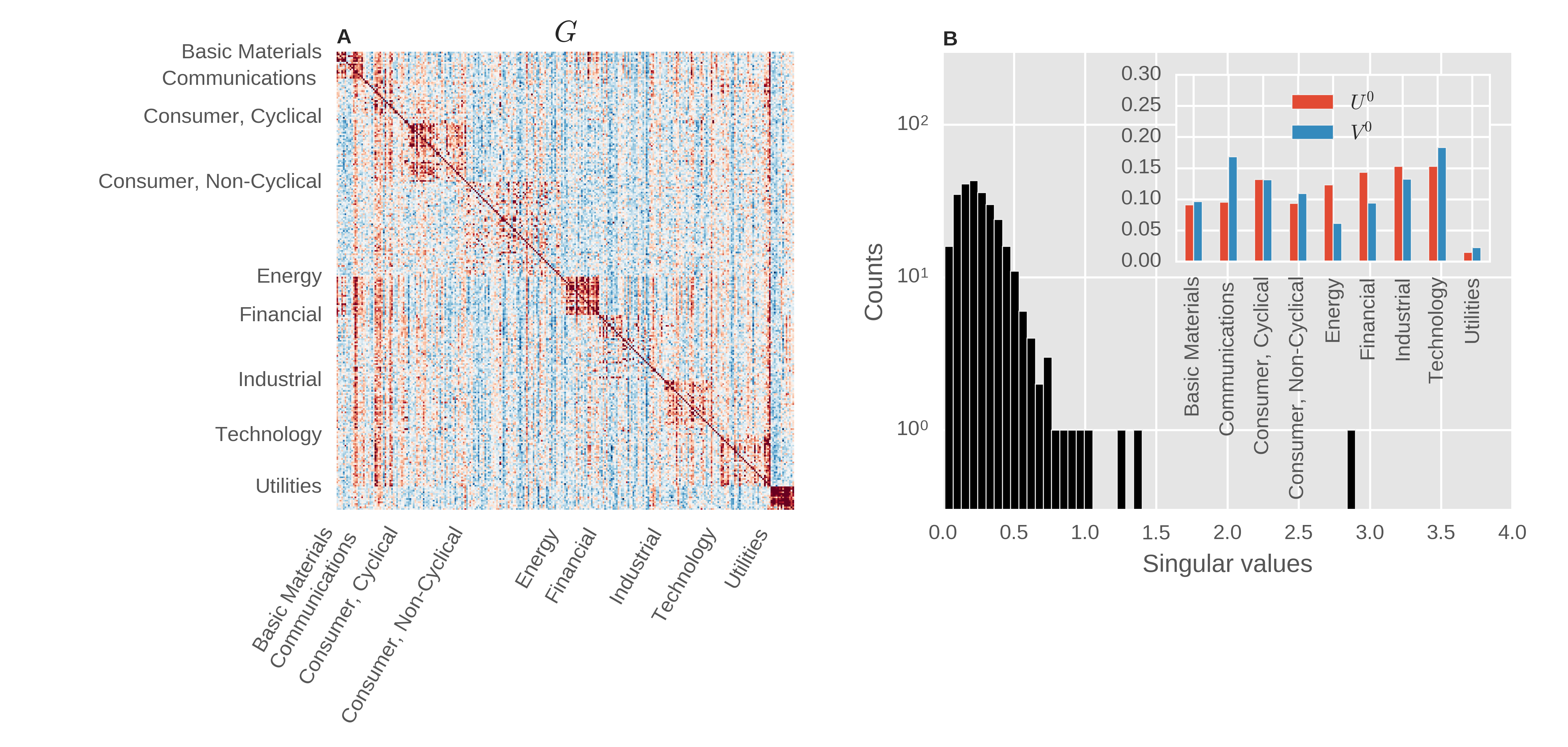
Figure 4: (a) Plot the propagator matrix $G^{ij}$ as obtained from the factorised scheme. (b) Histogram of singular values and composition of the ground singular vectors.

In order to address this issue more quantitatively, we introduce the singular-value decomposition of $G^{ij}$, defined as

$$G^{ij}=\sum_{a}U^{ia}S^{a}V^{ja}.$$ (10)

$U^{ia}$ and $V^{ia}$ are real orthogonal matrices, the columns of which correspond to the left/right singular vectors of $G^{ij}$, and where $S^{a}$ is a vector made of the corresponding singular values. The interpretation of the decomposition is straightforward: For a given $a$ the value $S^{a}$ is the increase of a linear combination $U^{ia}$ of stock prices after the combination of trades $V^{ia}$. Figure 4(b) displays the histogram of singular values $S^{a}$. Fig. 4(b) shows, among other things, that a market-neutral net imbalance has a smaller impact on prices than a directional one. In fact, due to $U^{i0}\approx V^{i0}\approx N^{-1/2}$ (see the inset of Fig. 4(b)), trading one standard deviation of the imbalance of the market mode costs roughly three standard deviations of its price, while all the other modes have a consistently smaller impact.

4.2 Response function and price covariation

Having found the propagator, we can investigate the interplay of $G^{ij}_{\tau}$ with $C^{ij}_{\tau}$ in shaping the response function and return correlation. In particular, within the propagator model one finds:

$$R^{ij}_{\tau} = \sum_{k}\Big{[}\sum_{\tau^{\prime}=0}^{\tau-1}G^{ik}_{\tau^{\prime}}c^{kj}_{\tau^{\prime}-\tau}+\sum_{\tau^{\prime}=\tau}^{\infty}\left(G^{ik}_{\tau^{\prime}}-G^{ik}_{\tau^{\prime}-\tau}\right)c^{kj}_{\tau^{\prime}-\tau}\Big{]}\ ,$$ (11)

and:

$$\Sigma^{ij}_{\tau} = \Sigma^{ij}_{G,\tau}+\Sigma^{ij}_{W,\tau}\ ,$$ (12)

where:

$$\Sigma^{ij}_{G,\tau} = \sum_{k,l}\Big{[}\sum_{\tau^{\prime},\tau^{\prime\prime}=0}^{\tau-1}G^{ik}_{\tau^{\prime}}c^{kl}_{\tau^{\prime}-\tau^{\prime\prime}}G^{jl}_{\tau^{\prime\prime}}+2\sum_{\tau^{\prime}=0}^{\tau-1}\sum_{\tau^{\prime\prime}=\tau}^{\infty}G^{ik}_{\tau^{\prime}}c^{kl}_{\tau^{\prime}-\tau^{\prime\prime}}\Big{(}G^{jl}_{\tau^{\prime\prime}}-G^{jl}_{\tau^{\prime\prime}-\tau}\Big{)}$$ (13)

$$\ \ \ \ \ \ \ \ \ \ \ \ \ \ \ \ \ \ +\sum_{\tau^{\prime},\tau^{\prime\prime}=\tau}^{\infty}\Big{(}G^{ik}_{\tau^{\prime}}-G^{ik}_{\tau^{\prime}-\tau}\Big{)}c^{kl}_{\tau^{\prime}-\tau^{\prime\prime}}\Big{(}G^{jl}_{\tau^{\prime\prime}}-G^{jl}_{\tau^{\prime\prime}-\tau}\Big{)}\Big{]}\ .$$

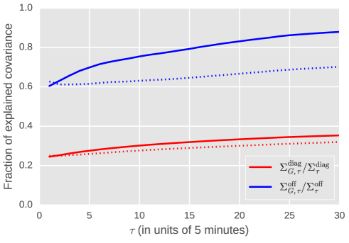
Figure 5: Plot of the fraction of explained diagonal and off-diagonal covariance as given by Eq. (12) as a function of the lag. The solid lines were obtained by extrapolating the sign correlation to infinity while the dotted lines are the result of truncating the past to a maximum lag equal to $T=30$.

This is an extension of the result found in Refs. [6, 12] in a linear equilibrium setting. The time-behavior of the first term $\Sigma^{ij}_{G,\tau}$ captures the dynamics of the model, that is very similar to the one found in the one-dimensional model. In that case, even if at large times $c_{\tau}\sim\tau^{-\gamma}$ with $\gamma\approx 0.5$, the long range dependence of the resulting propagator $G_{\tau}\sim\tau^{-\beta}$ with $\beta\approx 0.25$ is able to compensate the long-range dependence of the imbalances and restore the diffusivity of price, which indeed requires $\beta=(1-\gamma)/2$ [6, 1]. In this more general setting, as the time behavior of the model is found to be well-described by the factorized model (9), we are offered the same solution to reconcile the behavior of sign and return correlations. With these definitions, $\Sigma^{ij}_{G,\tau}$ denotes the part of the return covariance explained by the impact of transactions, while $\Sigma^{ij}_{W,\tau}$ stands for its unexplained component, for example due to news. Figure 5 displays the fraction of explained diagonal and off-diagonal covariance, which appears to increase with the lag. Interestingly, one can see that while only $\approx 25$-$35\%$ of the diagonal variance can be explained by impact, this figure rises to $\approx 60$-$90\%$ for its off-diagonal counterpart, meaning that the propagator model is somewhat more efficient to explain the covariance than it is to account for the variance. It is also interesting to mention that the propagator model is successful in reproducing the sectorial structure of the covariance matrix. For a visual interpretation, Fig. 6 displays plots of the three matrices that appear in Eq. (12).

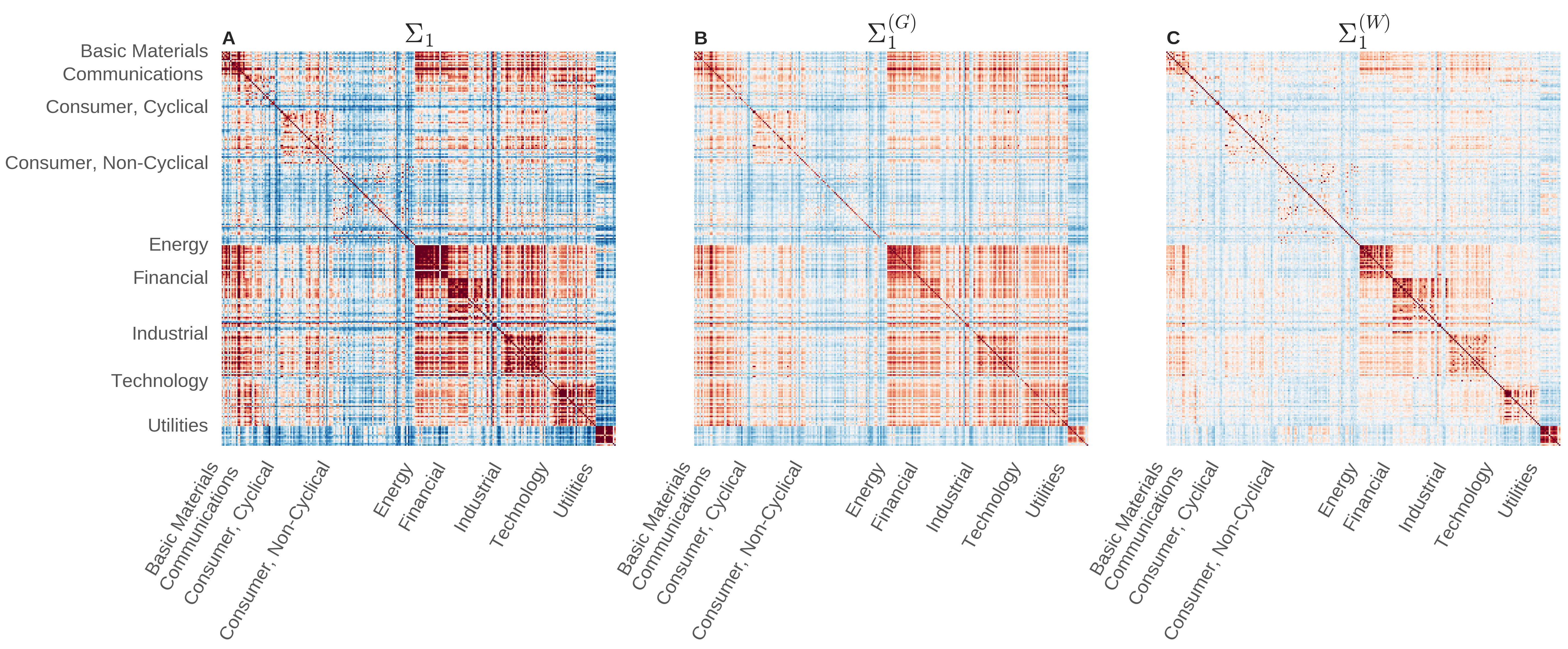
Figure 6: Plot of (a) the returns covariance matrix, (b) $\Sigma^{ij}_{G,\tau}$, and (c) $\Sigma^{ij}_{W,\tau}$, at lag $\tau=1$ (see Eq. (12)). Note that the matrices having been substracted of their mean for better visibility of their structure.

In order to assess whether the propagator model helps in understanding the direction of the risk modes of the market (and in particular, the composition of the sectors), we raise the following question: does $\Sigma^{ij}_{G,\tau}$ explain more of the price covariance structure than the sign covariance $C_{\tau}$ alone? To answer this quantitatively we compare the overlap of the eigenvectors of $\Sigma_{\tau}$ with those of $\Sigma_{G,\tau}$ and with those of $C_{\tau}$.

More precisely, if we denote the eigenvectors of these matrices by $U_{\Sigma},U_{C}$ and $U_{\Sigma_{G}}$, we have computed the overlap matrices $U^{T}_{\Sigma}U_{C}$ (see Figure 7(a)) and $U^{T}_{\Sigma}U_{\Sigma_{G}}$ (see Figure 7(b)). As one can see with the naked eye, the eigenmodes of $\Sigma_{\tau}$ have significantly larger overlap with $\Sigma_{G,\tau}$ than there is with $C_{\tau}$. Figure 7(c) displays a plot that captures quantitatively the latter statement and is constructed as follows: $(i)$ we crop each of the overlap matrices at $n\in\llbracket 1,N\rrbracket$, $(ii)$ compute their singular values $\{w_{a}\}_{a\in\llbracket 1,n\rrbracket}$ and sort them in decreasing order (the inset shows the singular value spectra at $n=50$), and $(iii)$ compute the so-called fraction of common modes $\left(\prod_{a=1}^{n}w_{a}\right)^{1/n}$ and plot it as a function of $n$. The dashed black line represents the theoretical expectation for the noise level [32]. This measure represents the volume of the common subspace spanned by the first $n$ eigenvectors, and is a very strict measure of similarity, which is why the results in Figure 7(c) are rather remarkable: one sees that the directional structure of the return covariance matrix can be predicted very well using liquidity variables only.

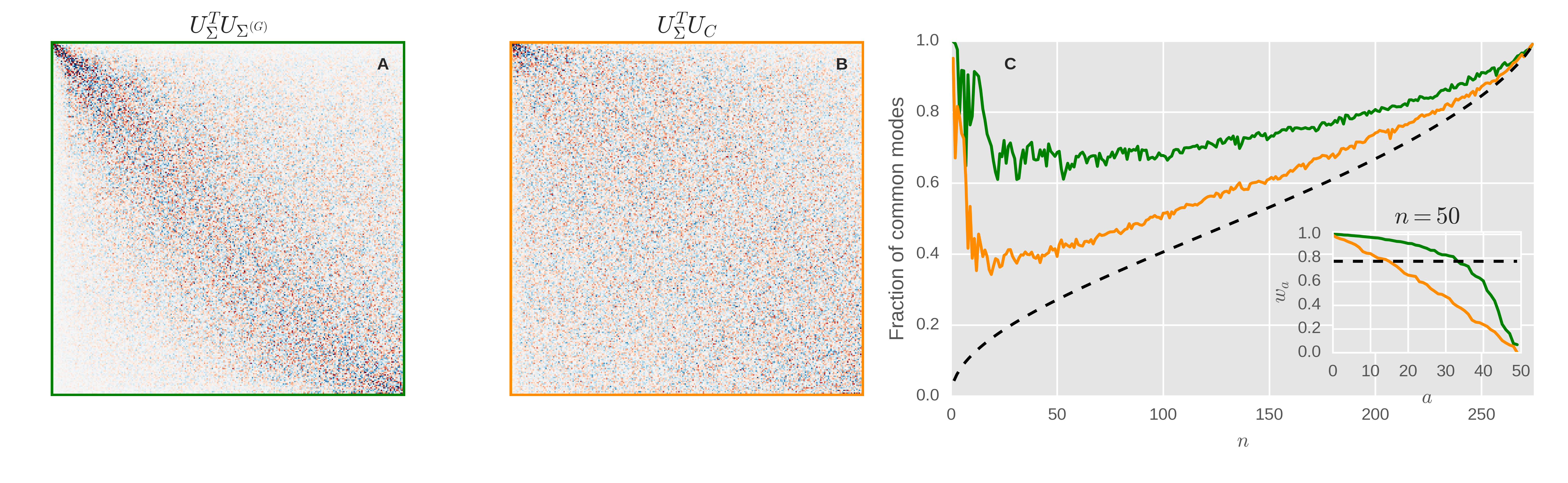
Figure 7: Plot of the overlap of eigen-rotation matrices of the returns covariance matrix with (a) $\Sigma^{ij}_{G,\tau}$ (see Eq. (12)), and (b) the sign covariance matrix. (c) Plot of the fraction of common modes as defined in the text.

4.3 Direct and cross-impact

A lot of the covariance and part of the variance come from impact, but how to measure the direct influence of impact versus its cross-sectional component? For the response $R^{ij}_{\tau}$ and covariance $\Sigma^{ij}_{G,\tau}$, one can simply use the following relations, which we have written in a diagrammatic way for the sake of readability. Note that the time structure has been omitted but can be easily recovered as each of the following terms has the temporal structure given in Eqs. (11) and (13). Red and blue filled circle signify returns and signs respectively. Empty circles imply exclusive sum over the products. Solid arrows represent propagators and dashed lines stand for sign correlations.

Below each term, we have indicated its relative contribution to the average self/cross-response/covariance. The interpretation of each term in the response is as follows:

a1

Self-response via direct impact. This is the classical term considered in most works on impact: trading in product $i$ impacts the price of $i$ itself.

a2

Self-response mediated by cross-trading and cross-impact. This term is induced by the order flow on all the stocks $k$ that are correlated to $i$. This causes market makers to include this extra information in their price for $i$.

b1

Cross-response mediated by cross-trading and direct impact. The mechanism is similar to a1, except that the order flow on $j$ now induces an imbalance on $i$, that translates into a price change via direct impact.

b2

Cross-response mediated by direct trading and cross-impact. Here the market markers react to the order flow on $j$ by updating their quotes on product $i$.

b3

Cross-response market mediated by cross-trading and cross-impact. Trading in a stock $j$ that is correlated with a large number of other stocks $k$. The market maker observes the order flow all of those, and adjusts his quote of $i$ based on this aggregate information.

Regarding the average weights of the different terms, it is interesting to notice that while most of the self-response can be explained through direct impact, this is no longer the case for the cross-response. For the latter, the dominating mechanism is b3, implying that most of the cross-response is mediated by delocalized modes (such as the market mode, or large sectors). This is one of the central message of this paper. Note that the same story can be told for the returns covariance with similar conclusions for the off-diagonal contribution.

4.4 Finite size scaling

As the main goal of this study is the characterization of the interactions among a large number of stocks, the fact that we only consider a sample of 275 instruments (whereas the US stock market amounts to several thousands of them), might seem restrictive. Such a relatively smaller sample implies that the order flow for all those missing products is – to us – unobserved, even though the interaction ($C$ and $G$) between stocks is on average positive. This may therefore lead to an overestimation of the magnitude of the propagators, which would then depend on system size.

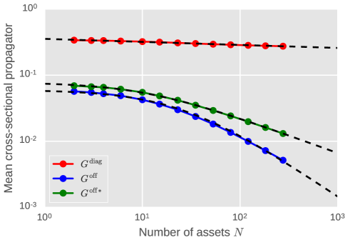
Figure 8: Plot of the mean diagonal ($G^{\mathrm{diag}}$) and off-diagonal ($G^{\mathrm{off}}$) propagators, as well as the mean of the off-diagonal elements where the traded and the impacted stock belong to the same sector ($G^{\mathrm{off}*}$). All curves are computed for $N$ stocks, as a function of $N$, and each data point results from the average of $10^{3}$ random bootstrap subsamples for each of which we perform cross-sectional propagator inversions.

In order to empirically verify this effect, we have fitted a factorized model as in Eq. (9) on many random subsets of stocks of variable size $N$. One would naively expect that the typical strength of direct impact propagators ($G^{ij}$ with $i=j$) be roughly constant regardless of $N$. On the other hand, cross propagators ($i\not=j$) are expected to decrease as $N^{-1}$ or faster, in order to avoid that their contribution ends up dominating over direct impact when $N\rightarrow\infty$.

The results are shown in Fig. 8. We can see that indeed $\left\langle G^{ij}\right\rangle_{i=j}$ decreases only very slightly with $N$ (fitting it to $k_{1}N^{-\nu_{1}}$ yields $k_{1}=0.36$ and $\nu_{1}=0.04$), while we get an excellent fit of cross terms $\left\langle G^{ij}\right\rangle_{i\not=j}={k_{2}}\big{(}{1+\frac{N}{N_{2}}}\big{)}^{-1}$, with $k_{2}=0.06$ and $N_{2}=24$ (see dashed lines in Fig. 8). This suggests a total asymptotic contribution of the off-diagonal propagators equal to $k_{2}N_{2}\approx 1.5$, to be compared to an average diagonal contribution of $\approx 0.3$.

We have also made a fit on the average of off-diagonal elements, conditioned such that $i$ and $j$ are in the same sector s: $\left\langle G^{ij}\right\rangle_{i\not=j;\mathrm{s}(i)=\mathrm{s}(j)}={k_{3}}\big{(}{1+\frac{N}{N_{3}}}\big{)}^{-\nu_{3}}$ gives $k_{3}=0.078$, $N_{3}=10.4$ and $\nu_{3}=0.54$. Pairwise cross-impact is naturally stronger in this case, than between two randomly selected stocks, since they are more likely to have a high correlation. Nevertheless, understanding how $\nu_{3}$ should behave is more delicate, as it requires estimating how the sizes of the sectors themselves scale with $N$.

5 Estimators of $G$: structure and statistical significance

5.1 The models

The model defined in Eq. (6) is a very general object, that is described by a propagator $G^{ij}_{\tau}$ of dimension $N^{2}\times T$, plus a covariance matrix $\sigma^{ij}_{W}$ of dimension $N^{2}$. Such an abundance of parameters results in the impossibility to estimate reliably the individual entries of $G^{ij}_{\tau}$ with the data in our possession. Only the aggregated statistics of $G^{ij}_{\tau}$ have been found statistically significant, see Fig. 4 and Table 1 below. We have thus decided to use a fully non-parametric estimation only in order to extract the main qualitative features of data. In order to estimate the interaction strengths $G^{ij}$ and investigate their structure in a more robust fashion, we have considered lower dimensional models.

More precisely, we have used three models in order to fit the propagators and we have compared their performance:

Fully non-parametric

The most general propagator model is specified the $N^{2}(T+1)$ parameters defining Eq. (6). This corresponds to the absence of any prior about the structure of the $G^{ij}_{\tau}$.

Factorized

A simpler model is obtained under the assumption $G^{ij}_{\tau}=G^{ij}\phi_{\tau}$, where $\phi_{\tau}$ given by Eq. (9). The dimensionality of the model is then reduced to $2N^{2}+T$.

Homogeneous

The simplest, non-trivial linear model for cross-impact is obtained by assuming

$$G^{ij} = \delta^{ij}G^{\mathrm{diag}}+(1-\delta^{ij})G^{\mathrm{off}},$$ (14)

$$\sigma^{ij}_{W} = \delta^{ij}\sigma^{\mathrm{diag}}_{W}+(1-\delta^{ij})\sigma^{\mathrm{off}}_{W}\ ,$$ (15)

so as to capture a single collective mode of the return covariance, corresponding to global market moves. The dimensionality of the model in this case is $4+T$. The estimators for this model are reported in the Appendix, and yield $G^{\mathrm{diag}}=0.29$ and $G^{\mathrm{off}}=0.0046$, consistent with the average diagonal and off-diagonal values of the previous model (see A.2).

All these models can be calibrated by minimizing their negative log-likelihood under a Gaussian assumption for the residuals $w^{i}_{t}$:

$$-\ln\mathcal{L}=\frac{T}{2}\ln\det\sigma_{W}+\frac{1}{2}\sum_{i,j,t}w^{i}_{t}w^{j}_{t}\left(\sigma_{W}^{-1}\right)^{ij},$$ (16)

allowing us to compute estimators for both the propagators $G^{ij}_{\tau}$ and the residual covariance matrix $\sigma^{ij}_{W}$. In this way, the estimated covariance matrix of the residual $\hat{\sigma}^{(W)}$ itself can be used in order to build metrics for the quality of the fit, and check how well the results generalize out-of-sample.

5.2 Discussion

The effort of fitting the propagator model under the different models described above can be justified by two different perspectives. On the one hand from the statistical point of view, it is desirable to avoid overfitting, so to have a robust model that generalizes well out-of-sample. This enables us to predict the future covariation of prices given the imbalances. On the other hand, from the informational point of view, one might prefer to compress the structure of the interaction in a small number of informative parameters, rather than dealing with a larger set of more anonymous coefficients. In order to quantitatively address these points, we have chosen to inspect the behavior of the residuals and of the likelihoods in all the three models, by defining three types of scores. The first two scores assess how well one is able to describe the fluctuations along the diagonal and the off-diagonal parts of the return covariance matrix (thus, they specify particular axes of the matrix $\sigma^{(W)}$ in which we are interested:

$$\mathcal{R}^{\mathrm{diag}} = \frac{\sum_{i}\hat{\sigma}_{W}^{ii}}{\sum_{i}\sigma^{ii}_{0}}=\frac{1}{N}\sum_{i}\hat{\sigma}_{W}^{ii},$$ (17)

$$\mathcal{R}^{\mathrm{off}} = \frac{\sum_{i\neq j}|\hat{\sigma}^{ij}_{W}|}{\sum_{i\neq j}|\sigma^{ij}_{0}|}.$$ (18)

Alternatively, the likelihood function automatically considers the fluctuations along the eigenmodes of $\sigma^{(W)}$, as its value is uniquely fixed by the eigenvalues of the residual covariance:

$$\mathcal{R}^{\ln\mathcal{L}} = -\frac{\ln\mathcal{L}}{NT}=\frac{1}{2}\left(1-\frac{1}{N}\log\det\hat{\sigma}_{W}\right).$$ (19)

Table 1 compares these scores for an in-sample period (2012) and an out-of-sample one (2013), in order to assess how each of the model generalizes to yet unseen data. Note that the in-sample scores are consistent with the results of Fig. 5 at lag $\tau=1$, indicating that the metrics that we have chosen provides a very conservative estimate of the model performance due to the increase of the predictive power with lag. We find that:

• All the in-sample scores improve by increasing the complexity of the models, as expected due to the fact that the models are nested. On the contrary, the good in-sample performance of the fully non-parametric model does not generalize out-of-sample. The scores displayed by the lower dimensional models are roughly the same in and out-of-sample, thus validating the practical use of the factorized and homogeneous propagator models.

• The quality in the reconstruction of the covariance of returns, measured by $\mathcal{R}^{\mathrm{off}}$, is better than the one of the variance. While the factorized model explains around 20% of the variance, it accounts for more than 50% of the covariance. This is compatible with the findings of Ref. [10] using a model with purely permanent impact.

• While both the factorized model and the homogeneous one have good out-of-sample performance, it is interesting to notice that thes factorized model has a consistently better $\mathcal{R}^{\mathrm{off}}$ score. This is consistent with our previous results (see Fig. 7), indicating that the directional structure of the matrix $G^{ij}$ is statistically significant, and allows one to explain a consistent part of the return covariation.

The good out-of-sample performance also indicates that heterogeneities in the temporal behaviour of the propagator discussed in Section 4.1 are weak enough for these models to generalize well across years.

Table 1: Table of scores for the three models described in Sec. 5.

	in-sample (2012)			out-of-sample (2013)
Model	$\mathcal{R}^{\mathrm{diag}}$	$\mathcal{R}^{\mathrm{off}}$	$\mathcal{R}^{\ln\mathcal{L}}$	$\mathcal{R}^{\mathrm{diag}}$	$\mathcal{R}^{\mathrm{off}}$	$\mathcal{R}^{\ln\mathcal{L}}$
Non-parametric	0.437	0.185	0.466	2.08	1.312	1.187
Factorised	0.748	0.374	0.744	0.79	0.454	0.762
Homogeneous	0.819	0.484	0.841	0.786	0.628	0.81

6 Conclusions

The treatment of cross-impact in the existing literature has been scarce at best [10, 12, 13, 14], despite its importance – in our opinion – to correctly estimate the liquidation costs of a diversified portfolio. In this work we have attempted to give a more complete picture of such effects by decomposing them using a simple, linear propagator approach. Our dynamical model explains rather well the off-diagonal elements of the correlation matrix, which makes us conclude that to a large extent, cross-correlations between different stocks are mediated by trades. Market makers/HFT liquidity providers learn from correlated order flow on multiple instruments, and adjust their prices at a portfolio level. This allows them to better adapt to global movements in the market, and to reduce the amount of adverse selection they are faced with. Such an observation is underpinned by the good fit of our homogeneous model, where each stock reacts to the total, net order flow of the others. This focus of market makers/HFT on their net inventory is consistent with the idea that being uniformly long or short across stocks is much more risky than to be long-short by same gross amount in a diversified fashion.

In the present study we took an empirical, descriptive point of view regarding price reaction and market maker behavior. In particular, we have disregarded the strong implications that these results have in the context of optimal execution, that will be the object of a forthcoming paper [35].

We wish to thank R. Benichou, J. Bun, A. Darmon, L. Duchayne, S. Hardiman, J. Kockelkoren, J. de Lataillade, C.-A. Lehalle, F. Patzelt, E. Sérié and B. Tóth for very fruitful discussions.

Appendix A Models

It is important to mention that while the results in this paper are presented with integrated response functions $R^{ij}_{\tau}$ and propagators $G^{ij}_{\tau}$, all propagator inversions have been done with differential response functions $r^{ij}_{\tau}$. This is consistent with the idea that such quantities have a decaying asymptotic behaviour in contrast with their integrated counterparts and thus suffer less from the cut-off effect [36, 30]. The integrated propagator was then computed by using the relation $G^{ij}_{\tau}=\sum_{\tau^{\prime}=1}^{\tau}g^{ij}_{\tau^{\prime}}$. Figure 9 displays the diagonal and off-diagonal means of the lagged sign correlation function, the lagged return correlation function and the differential response function.

A.1 Fully non-parametric model

The maximization of the likelihood function (16) of the model in the fully non-parametric case yields a well-known matrix equation for the propagator:

$$\hat{r}^{ij}_{\tau}=\sum_{k}\sum_{\tau^{\prime}=0}^{T-1}\,\hat{g}^{ik}_{\tau^{\prime}}\,\hat{c}^{kj}_{\tau,\tau^{\prime}}\ ,$$ (20)

that is defined in terms of the (biased) estimators for, respectively, the differential response and the sign correlation:

$$\hat{r}^{ij}_{\tau} = \frac{1}{T}\sum_{t,t^{\prime}=1}^{T}x^{i}_{t}\varepsilon^{j}_{t^{\prime}}\delta(t-t^{\prime}-\tau)$$ (21)

$$\hat{c}^{ij}_{\tau,\tau^{\prime}} = \frac{1}{T}\sum_{t,t^{\prime},t^{\prime\prime}=1}^{T}\varepsilon^{i}_{t^{\prime}}\varepsilon^{j}_{t^{\prime\prime}}\delta(t-t^{\prime}-\tau)\delta(t-t^{\prime\prime}-\tau^{\prime})\ .$$ (22)

In order to reduce noise and facilitate matrix inversion, we’ve assume stationarity, so that we define the following stationary estimator for the sign correlation, in which we enforce a Toeplitz structure:

$$\hat{c}^{ij}_{\tau-\tau^{\prime}} = \frac{1}{T}\sum_{t,t^{\prime}=1}^{T}\varepsilon^{i}_{t}\varepsilon^{j}_{t^{\prime}}\delta(t-t^{\prime}-\tau)\ .$$ (23)

so that Eq. (20) becomes a simpler convolution. The estimator of the residuals is also straightforward to compute:

$$\hat{\sigma}^{ij}_{W}=\frac{1}{T}\sum_{t=1}^{T}w^{i}_{t}w^{j}_{t}\,.$$ (24)

The total number of parameters to estimate under this method is $N^{2}(T+1)$, while the computational bottleneck results from the inversion of the block-Toeplitz matrix $c^{ij}_{\tau}$ appearing in Eq. (24).

A.2 Factorized model

The assumption of a propagator of the form

$$G^{ij}_{\tau} = G^{ij}\phi_{\tau}\,,$$ (25)

where $\phi_{\tau}$ is given by Eq. (9), results in a simpler estimation of $N^{2}+T$ parameters for the kernel and $N^{2}$ parameters for the residuals. The estimator for the propagator is found by solving:

$$\hat{G}^{ij}=A\left(B^{T}\right)^{-1}\,,$$ (26)

where one has preliminarily defined:

$$A^{ij} = \sum_{\tau}\hat{R}^{ij}_{\tau}\phi_{\tau}$$ (27)

$$B^{ij} = \sum_{\tau,\tau^{\prime}}\hat{c}^{ij}_{\tau-\tau^{\prime}}\phi_{\tau}\phi_{\tau^{\prime}}\,,$$ (28)

whereas the estimator of the variance is given by the earlier expression (24).

A.3 The homogeneous model

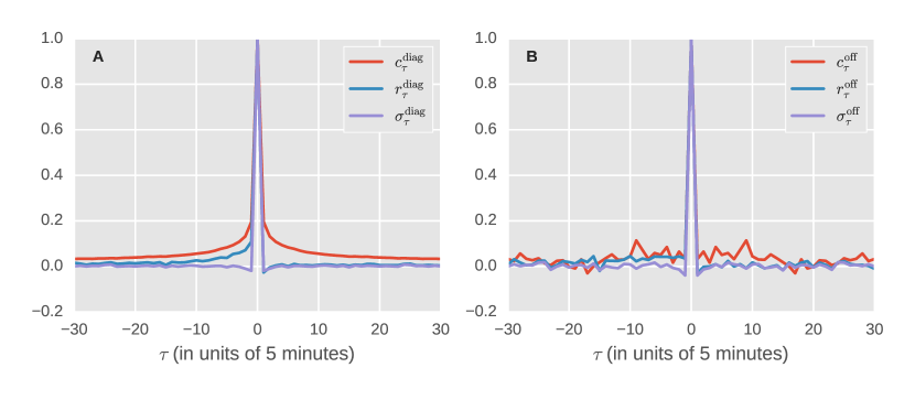
Figure 9: Plot of the diagonal (a) and off-diagonal (b) means of the lagged sign correlation function, the returns lagged correlation function and the differential response function.

The estimator for the propagator reads

$$\hat{G}^{\mathrm{diag}} = \frac{1}{N}\left(\frac{A^{\mathrm{M}}}{B^{\mathrm{M}}}+(N-1)\frac{A^{\mathrm{M}}-A^{\mathrm{I}}}{B^{\mathrm{M}}-B^{\mathrm{I}}}\right)\,,$$ (29)

$$\hat{G}^{\mathrm{off}} = \frac{1}{N}\left(\frac{A^{\mathrm{M}}}{B^{\mathrm{M}}}-\frac{A^{\mathrm{M}}-A^{\mathrm{I}}}{B^{\mathrm{M}}-B^{\mathrm{I}}}\right)\,,$$ (30)

where one has preliminarily defined the market (M) and idiosyncratic (I) means:

$$A^{\mathrm{M}} = \mathbb{E}[A^{ij}]=\frac{1}{N^{2}}\sum_{ij}A^{ij}\,,$$ (31)

$$A^{\mathrm{I}} = \mathbb{E}[A^{ii}]=\frac{\mathrm{Tr}[A]}{N}\,,$$ (32)

and equivalently for $B^{\mathrm{M}}$ and $B^{\mathrm{I}}$. The estimator of the variance is given by (we give the inverse of the estimator for simplicity):

$$\left(\hat{\sigma}_{W}\right)^{-1,\mathrm{diag}} = \frac{1}{N}\left(\lambda^{\mathrm{M}}+(N-1)\lambda^{\mathrm{I}}\right)\,,$$ (33)

$$\left(\hat{\sigma}_{W}\right)^{-1,\mathrm{off}} = \frac{1}{N}\left(\lambda^{\mathrm{M}}-\lambda^{\mathrm{I}}\right)\,.$$ (34)

We have also introduced

$$\lambda^{\mathrm{M}} = \frac{1}{N}\left[\mathbb{E}[\sigma_{0}]-\frac{{A^{\mathrm{M}}}^{2}}{B^{\mathrm{M}}}\right]^{-1}\,,$$ (35)

$$\lambda^{\mathrm{I}} = \frac{N-1}{N}\left[1-\mathbb{E}[\sigma_{0}]+\frac{\left(A^{\mathrm{M}}-A^{\mathrm{I}}\right)^{2}}{B^{\mathrm{M}}-B^{\mathrm{I}}}\right]^{-1}\ .$$ (36)

References

- [1] Bouchaud J P, Farmer J D and Lillo F 2008 How markets slowly digest changes in supply and demand (Elsevier: Academic Press)
- [2] Hasbrouck J 1988 Journal of Financial Economics 22 229–252
- [3] Hasbrouck J 1991 The Journal of Finance 46 179–207
- [4] Jones C M, Kaul G and Lipson M L 1994 Review of Financial Studies 7 631–651
- [5] Dufour A and Engle R F 2000 The Journal of Finance 55 2467–2498
- [6] Bouchaud J P, Gefen Y, Potters M and Wyart M 2004 Quantitative Finance 4 176–190
- [7] Lillo F and Farmer J D 2004 Studies in Nonlinear Dynamics & Econometrics 8
- [8] Eisler Z, Bouchaud J P and Kockelkoren J 2012 Quantitative Finance 12 1395–1419
- [9] Bacry E and Muzy J F 2014 Quantitative Finance 14 1147–1166
- [10] Hasbrouck J and Seppi D J 2001 Journal of financial Economics 59 383–411
- [11] Boulatov A, Hendershott T and Livdan D 2013 The Review of Economic Studies 80 35–72
- [12] Pasquariello P and Vega C 2013 Review of Finance 19 229–282
- [13] Wang S, Schäfer R and Guhr T 2016 arXiv:1603.01586
- [14] Wang S, Schäfer R and Guhr T 2016 The European Physical Journal B 89 1–16
- [15] Mastromatteo I, Toth B and Bouchaud J P 2014 Physical Review E 89 042805
- [16] Markowitz H 1952 The Journal of Finance 7 77–91
- [17] Meucci A 2009 Risk and asset allocation (Springer Science & Business Media)
- [18] Epps T W 1979 Journal of the American Statistical Association 74 291–298
- [19] Tóth B and Kertész J 2009 Quantitative Finance 9 793–802
- [20] Tóth B and Kertész J 2006 Physica A: Statistical Mechanics and its Applications 360 505–515
- [21] Large J 2007 Unpublished paper: Oxford-Man Institute, University of Oxford
- [22] Bacry M and Muzy J F 2014 Quantitative Finance 14
- [23] Laloux L, Cizeau P, Bouchaud J P and Potters M 1999 Physical Review Letters 83 1467
- [24] Bonanno G, Lillo F and Mantegna R N Quantitative Finance 1 96–104
- [25] Marsili M 2006 Quantitative Finance 2 297–302
- [26] Allez Romain B J P 2011 New Journal of Physics 13 025010
- [27] Marčenko V A and Pastur L A 1967 Mathematics of the USSR-Sbornik 1 457
- [28] Bouchaud J P and Potters M 2011 Financial applications of random matrix theory: a short review (Oxford University Press)
- [29] Bouchaud J P, Kockelkoren J and Potters M 2006 Quantitative Finance 6 115–123
- [30] Eisler Z, Bouchaud J P and Kockelkoren J 2011 Available at https://ssrn.com/abstract=1888105 and Market Microstructure: Confronting Many Viewpoints, Wiley (2013)
- [31] Taranto D E, Bormetti G, Bouchaud J P, Lillo F and Tóth B 2016 arXiv:1602.02735
- [32] Bouchaud J P, Laloux L, Miceli M A and Potters M 2007 The European Physical Journal B 55 201–207
- [33] Taranto D E, Bormetti G, Bouchaud J P, Lillo F and Tóth B 2016 arXiv:1604.07556
- [34] Dayri K and Rosenbaum M 2015 Market Microstructure and Liquidity 1 1550003
- [35] Mastromatteo I, Benzaquen M, Eisler Z and Bouchaud J P 2016 (in preparation)
- [36] Sérié E 2010 Unpublished report, Capital Fund Management, Paris, France