Analysis of Artificial Dissipation of Explicit and Implicit Time-Integration Methods
Abstract
Stability is an important aspect of numerical methods for hyperbolic conservation laws and has received much interest. However, continuity in time is often assumed and only semidiscrete stability is studied. Thus, it is interesting to investigate the influence of explicit and implicit time integration methods on the stability of numerical schemes. If an explicit time integration method is applied, spacially stable numerical schemes for hyperbolic conservation laws can result in unstable fully discrete schemes. Focusing on the explicit Euler method (and convex combinations thereof), undesired terms in the energy balance trigger this phenomenon and introduce an erroneous growth of the energy over time. In this work, we study the influence of artificial dissipation and modal filtering in the context of discontinuous spectral element methods to remedy these issues. In particular, lower bounds on the strength of both artificial dissipation and modal filtering operators are given and an adaptive procedure to conserve the (discrete) norm of the numerical solution in time is derived. This might be beneficial in regions where the solution is smooth and for long time simulations. Moreover, this approach is used to study the connections between explicit and implicit time integration methods and the associated energy production. By adjusting the adaptive procedure, we demonstrate that filtering in explicit time integration methods is able to mimic the dissipative behavior inherent in implicit time integration methods. This contribution leads to a better understanding of existing algorithms and numerical techniques, in particular the application of artificial dissipation as well as modal filtering in the context of numerical methods for hyperbolic conservation laws together with the selection of explicit or implicit time integration methods.
keywords:
hyperbolic conservation laws, flux reconstruction, summation-by-parts, artificial viscosity, fully discrete stability, time integration methodsAMS subject classification. 65M12, 65M20, 65M60, 65M70
1 Introduction
Stability is one of the main desirable properties for a numerical scheme to solve hyperbolic conservation laws. This is due to the fact that at least for linear symmetric systems, an energy estimate (and the correct number of boundary conditions for initial boundary value problems) comes along with uniqueness and existence of a solution [21]. In the last years, several approaches have been proposed to construct entropy stable/conservative schemes like in [54, 53, 47, 42, 36, 13, 56, 3, 2, 9, 8, 11] and references therein. Recently, Abgrall [2] presented a way to build entropy stable/conservative schemes using the Residual Distribution (RD) framework. In [4], this idea is extended to Flux Reconstruction (FR) methods. This idea is fairly general and has been extended and re-interpreted in the discontinuous Galerkin (DG) context in [5]. However, besides the spacial discretization, the selection of the time integration method is essential for stability of these methods.
First of all, one has to choose between explicit or implicit methods to march forward in time. Implicit methods have favorable stability properties and, in particular, allow larger time steps. For instance, by using implicit time integration methods build on Summation-By-Parts (SBP) operators in time111These schemes can be interpreted as implicit Runge-Kutta (RK) methods [6, 43]. [34], the semidiscrete stability results transfer directly to the fully discrete case [32, 33, 12]. It should be stressed, however, that implicit methods yield to (typically non-)linear systems to be solved. Since the time step is also constrained by accuracy requirements, implicit methods may not be as efficient as explicit ones.
Explicit time integration methods, on the other hand, can be faster and easier to implement, but suffer from stability issues triggered by additional error terms. One way to improve the stability properties of numerical schemes is the usage of artificial dissipation. This idea dates back to early works of von Neumann and Richtymer [55]. Since then, many researchers have contributed to the development and extension of artificial dissipation methods, including the works [54, 52, 29, 31, 44].
In this work, we investigate the connections between artificial dissipation in explicit time integration methods and implicit time integration methods without additional limiting from point of stability. We further extend this investigation to modal filtering. Modal filtering is strongly connected to artificial dissipation methods in spectral and spectral element methods [30, 17, 25, 18, 7, 38] and provides an alternative which, in some cases222For instance, when the method is already formulated in a suitable modal basis., might be more efficient and easier to implement. In particular, we demonstrate that it is possible to mimic the dissipation (and thus stability) inherent in implicit time integration methods for explicit time integration methods when modal filtering with a suitable filter strength is incorporated. This result directly carries over to explicit time integration methods with suitable artificial dissipation terms. Thus, we are able to present an approach to obtain stable fully discrete schemes using explicit time integration. Such discretizations combine the favorable stability properties of implicit time integration methods with the efficiency gain of explicit time integration methods. Finally, we would like to mention that recently a relaxation Runge-Kutta approach has been proposed to construct fully discrete explicit energy (entropy) conservative/stable schemes in [23, 48]. Their approach has some similarities to our consideration but instead of working with modal filters or artificial viscosity to destroy the energy production in time, they change the final update step in the RK method to guarantee that the discrete energy equality is fulfilled.
For sake of simplicity, the explicit Euler method is considered. Yet, at least for non-linear problems, the same stability issues arise for strong stability preserving (SSP) RK schemes, since they can be written as convex combination of explicit Euler steps [19]. In the appendix, we show how our investigation carries over to general Runge-Kutta methods. Recent relevant articles concerned with the strong stability of explicit Runge-Kutta methods are, e.g., [50, 51, 27, 28, 41, 45].
The rest of this work is organized as follows: In section 2, we start by briefly revisiting the FR method in its formulation using SBP operators. This method yields a stable semidiscretisation and thus serves as a representative of a stable scheme. Yet, the examinations are rather general and valid for other spacial discretizations as well. In section 3, we investigate the mechanism which triggers stability issues when semidiscretisation (even stable ones) are evolved in time by explicit time marching. Further, we investigate the stabilizing effect of artificial dissipation terms and modal filtering. In principle, similar investigations are well-known. Performing this analysis in a vector matrix-vector representation including suitable discrete inner products, however, we are able derive new (strict) bounds on the artificial viscosity strength and filter strength for stability to carry over in time. Building up on this strategy, adaptive filtering strategies can be derived which yield methods with neither not enough nor too much dissipation. This might be beneficial in smooth regions for long time simulations. Section 4 explores the connection between implicit time integration and modal filtering in explicit time integration. We end this work by a summary in section 5. In the appendix, we demonstrate how the investigation for the filter strength of section 3 can be extended to general Runge-Kutta methods.
2 Flux Reconstruction using Summation-By-Parts Operators
In this section, we provide a brief description of FR methods using SBP operators, which will serve as a representative for spacially stable methods in the later investigations. Yet, it should be stressed that our analysis is also valid for other space discretisation, such as like DG or finite volume (FV) schemes. Further, let us consider a one-dimensional scalar conservation law
| (1) |
on , equipped with adequate boundary and initial conditions. For sake of simplicity, in this work, periodic boundary conditions will be assumed.
The domain is partitioned into smaller subdomains, also called elements, which are mapped diffeomorphically onto a reference element, typically . All calculations are conducted within this reference element then. There, the solution is approximated by a polynomial of degree . Let be a set of interpolation points in . Then, can be represented w.r.t. to a nodal Lagrange basis, resulting in a vector of coefficients given by for .
Note that the representation of w.r.t. other bases is possible as well. In the setting described in [46], the solution is represented as an element of a finite dimensional Hilbert space of functions on the volume. W.r.t. a chosen basis, the scalar product approximating the scalar product is represented by a matrix and the derivative (divergence) by . Additionally, functions on the boundary (consisting of two points in this one dimensional case) are elements of another finite dimensional Hilbert space with appropriate basis. The restriction of functions on the volume to the boundary is represented by a (rectangular) matrix and integration w.r.t. the outer normal by . Finally, the operators have to fulfil the SBP property
| (2) |
as a compatibility condition in order to mimic integration by parts
| (3) |
Additional ingredients of FR methods are numerical fluxes (Riemann solvers) , computing a single valued flux on the boundary using values from both neighbouring elements, and a correction step which can be formulated as a Simultaneous-Approximation-Term (SAT) from finite difference (FD) methods [47]. An overview and translation rules linking the notation used in this article and in DG or FD methods can be found in [40].
In the following, either nodal Gauß-Legendre and Lobatto-Legendre or modal Legendre bases will be used. Multiplication of functions on the volume will be conducted pointwise for nodal bases or exactly, followed by an projection, for modal bases. The resulting multiplication operators are written with two underlines, e.g. represents multiplication with the polynomial given by .
Example 2.1.
We give two examples for the discretisation. The linear advection with constant velocity is given by
| (4) |
The semidiscretisation using the canonical choice for the correction procedure can be written as
| (5) |
in the reference domain. The second example, which we also consider later is the nonlinear Burgers’ equation
| (6) |
This is more difficult, since discontinuities may develop in finite time. A discretisation is given by a skew symmetric form
| (7) |
Using (5) or (7) results in spacially stable schemes if an appropriate numerical flux is applied, see [47].
3 Artificial Dissipation and Modal Filtering
In this section, we investigate the stabilising effect of artificial dissipation operators and modal filtering. We note that both techniques share a strong connection. Using a first order operator splitting in time, artificial dissipation operators can be interpreted as exponential modal filter, see [38, 17, 44, 16].
In artificial dissipation methods, a small (super) diffusive term of even order is added to the conservation law (1). This yields
| (8) |
where is the order, the strength, and is a suitable function. The term describes the -fold application of the linear operator . Henceforth, the dependence on and will be implied but not written explicitly in all cases.
3.1 Discrete Formulation
In order to get a working numerical scheme, a time discretisation has to be introduced. For simplicity, we start by considering an explicit Euler method. Yet, once stability is ensured for the simple explicit Euler method, this result carries over to the whole class of explicit SSP-RK methods under appropriate time step restriction. This is, for instance, described in the monograph [19] and references cited therein.
In the standard element, one time step by the explicit Euler method is given by
| (9) |
Using an SBP-FR semidiscretisation to compute the time derivative in (9) without artificial viscosity, the norm after one Euler step is given by
| (10) | ||||
Here, the second term on the right hand side, , yields only boundary terms that can be controlled by the numerical flux. However, the last term, , is non-negative and might therefore increase the norm. It is this term, which is responsible for (spacially stable) methods to still become unstable in time. In the following subsections, we investigate two approaches to remedy this source of instability.
3.2 Application of Artificial Viscosity
We now derive a lower bound on the strength for artificial dissipation to carry spacial stability of a method over to time. Assuming a fixed function and order , the strength can be estimated in the following way. Denoting the time derivative obtained by the underlying SBP-FR method without artificial dissipation by and the matrix representation of the discretised artificial dissipation by
| (11) |
yields
| (12) |
Note that other discretisations of the artificial viscosity term in (8) are possible but not recommended. Yet, it has been proved in [44] that the discretisation (11) is compatible with SBP operators and results in dissipation of the -entropy. Thus, after one time step by the explicit Euler method with artificial dissipation, the norm is given by
| (13) | ||||
Again, can be estimated in terms of boundary values and numerical fluxes and is negative (non-positive) for a spacially stable discretisation of (1). Hence, for the method to be stable in time, the two last terms need to cancel out. In this case,
| (14) |
would follow and the fully discrete scheme will be conservative as well as stable in space and time. Using (13), the condition of the last to terms to cancel out can be rewritten as
| (15) | ||||
which again is equivalent to
| (16) |
The (possibly complex) roots of the equation (16) for are given by
| (17) |
Hence, for a sufficiently small time step and if the solution is not constant, the discriminant is non-negative and there is at least one real solution . Additionally, both and are positive for sufficiently small , since the artificial dissipation operator is positive semi-definite, i.e.
| (18) |
Thus,
| (19) |
and the roots of the quadratic equation (16) are non-negative. These results are summed up in the following
Lemma 3.1.
If a conservative and stable SBP-FR method for a scalar conservation law is augmented with the artificial dissipation on the right hand side, the fully discrete scheme using an explicit Euler method as time discretisation is both conservative and stable if
-
•
a nodal Gauß-Legendre / Lobatto-Legendre or a modal Legendre basis is used,
-
•
, which will be fulfilled for the choice of described below if the solution is not constant,
-
•
the time step is small enough such that (18) is fulfilled,
-
•
and the strength is big enough.
In our implementation, the strength of dissipation is chosen as the second (smaller) root and results in methods with highly desired stability properties, as we presented in numerical tests at the end of this section.
Remark 3.2.
It remains an interesting, yet unanswered, question how to interpret the existence of an additional solution . Since this solution yields a larger strength, the resulting methods show higher dissipation, which might be undesired in elements without discontinuities or for long time simulations [35, 37].
Note that the CFL condition and therefore the time step in an explicit time integration method depends on the parameters of the viscosity term. If no care is taken, artificial dissipation operators will decreases the allowable time step size; see [20, 24, 16] and references therein. Additionally, equation (18) limits the maximal time step and can be used as an adaptive strategy to control this quantity. This could be also used for an adaptive control strategy and will be considered in future investigations. Here, a simple limiting strategy is used for the numerical experiments. If the time step is not small enough and equation (18) is not fulfilled, the strength computed from (20) might be negative. In this case, to avoid instabilities, is set to zero, i.e. no artificial viscosity is used in the corresponding elements. This phenomenon is strongly connected with stability requirements of the artificial dissipation operator, which have been discussed above. Considering a time step by the explicit Euler method for the equation , the norm after one time step satisfies
| (21) | ||||
Thus, in order to guarantee , for , has to be limited by
| (22) |
Since is a second-order derivative operator, this yields a restriction on the time step of order . However, it should be noted that is computed using the given value of and is typically small.
3.3 Usage of Modal Filters
In this subsection, we investigate stability of the explicit Euler method combined with modal filtering, which is strongly related to artificial dissipation [30, 25, 18, 7, 17, 44, 16]. In certain cases, for instance when the method is already formulated w.r.t. a suitable modal basis, modal filtering can be more efficient and easier to implement than artificial dissipation. Further, no additional time step restrictions are introduced. For modal filtering, an operator splitting approach is applied together with an explicit Euler method. The update reads
| (23) |
where (9) holds for instead of and is the modal filter. If the filter reduces the norm of by the amount of the additional term , the fully discrete scheme allows the same estimate as the semidiscrete one. Therefore, similar to artificial dissipation, the modal filter has to eliminate the additional positive term. This idea is summarised in
Lemma 3.3.
Rendering a conservative and stable semidiscretisation of the scalar conservation law (1) fully discrete by using an explicit Euler step with modal filtering (23) yields a conservative and stable scheme if
| (24) | ||||
This condition can be fulfilled (per element) if
-
•
the rate of change is zero or
-
•
the intermediate value is not constant and the time step is small enough.
In order to fulfil condition (24) of Lemma 3.3, the filter strength (with time step included) has to be adapted. Using a modal Legendre basis, the (exact) modal filter can be written as
| (25) |
where as it is derived in [44]. For stability, the selection of the free parameter is essential. Similar to subsection 3.2, we now derive a lower bound on the filter strength that ensures stability. Representing the polynomial given by in a modal Legendre basis, i.e. as a linear combination of Legendre polynomials , condition (24) translates to
| (26) |
where the right-hand side is abbreviated as . Using the well-known inequality
| (27) |
as a first order approximation, can be estimated by
| (28) | ||||
for . Note that we have if and only if is not identically zero. Inserting
| (29) | ||||
this yields
Lemma 3.4.
A necessary condition for the filter strength according to Lemma 3.3 is
| (30) |
Remark 3.5.
By applying estimation (30) in our numerical scheme, an adaptive strategy can be applied. Note that other approximations than (27) could be used. The same is true if, instead of the explicit Euler method, an (explicit) SSP time integration method is applied, since such methods can be written as a convex combinations of steps by the explicit Euler method [19], and the filter is applied after each Euler step. An extension to some Deferred Correction (DEC) methods can also be done, since one can write some of theses methods likewise as convex combinations of Euler steps [26, 1]. However, since the triangle inequality is invoked for the resulting estimates, an undesired additional decrease of the norm may result. Therefore, the adaptive modal filtering should be applied only after a full time step and not for every stage. This was for instance demonstrated in [44]. Further, this renders the computation more efficient. Nevertheless, an extension of this approach to classical Runge-Kutta methods can be done, yielding to some further conditions which we present in the appendix Appendix.
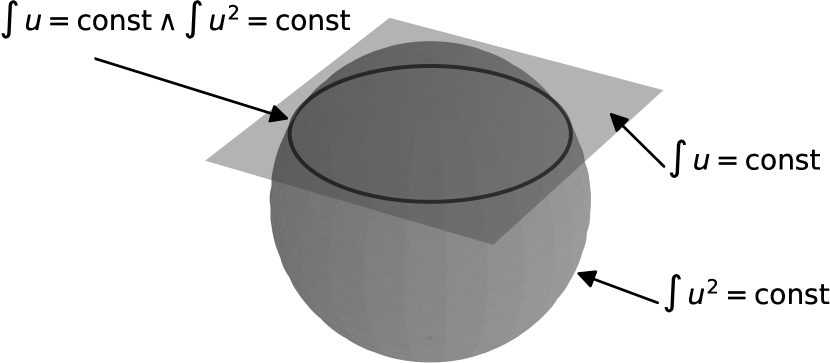
Finally, it should be stressed that adaptive modal filtering can be interpreted as a special case of projection, enforcing the constraint on the squared norm (a quadratic form) and not violating conservation, i.e. a constraint on the integral of the solution (a linear form). This is visualised in Figure 1. However, there are various possibilities to conduct this projection. As noted in section IV.4 of [22], projection methods can be useful, but can also destroy good properties. Therefore, they have to be investigated thoroughly.
Remark 3.6 (Connection to Relaxation RK approach).
In our analysis, we describe the production of energy in equation (10). Here, artificial viscosity or modal filters are applied to remove the additional energy. In [23, 48], the idea is instead to manipulate the time step such that the energy remains constant. This can be interpreted as a projection in the direction of the step update which conserves the energy and all linear invariants. In this article, we use different kinds of projections, e.g. ones given by modal filters, which also preserve important linear invariants such as the total mass.
3.4 Numerical Simulations
We close this section with a numerical demonstration of the above results and derived adaptive filtering strategies.
Comparing Modal Filtering and Projection
As an example, the linear advection equation with constant coefficients
| (31) |
in with periodic boundary conditions is considered. For the spacial discretisation, we choose a grid of elements using polynomials of degree and an upwind numerical flux.
At first, we consider a smooth initial condition
| (32) |
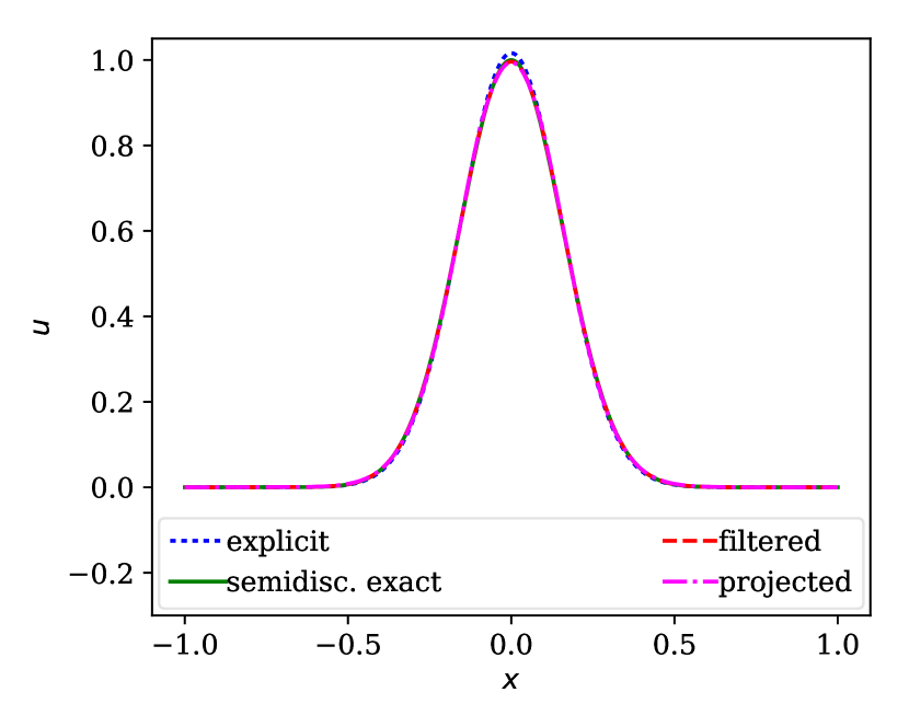
and simulate in the time interval using time steps of the explicit Euler method, the explicit Euler method with adaptive modal filtering, and the explicit Euler method with a simple projection. The simple projection is given by a scaling of all the non-constant Legendre modes by the same factor, resulting in the desired norm inequality and conservation. In 2(a), we realise that the projection is not really necessary, the results are very similar to the ones of the filtered method and all solutions are visually nearly indistinguishable. Using high order Runge-Kutta schemes does not lead to other observations for this test case.

However, for the non-smooth initial data
| (33) |
the same simulation results in Gibbs oscillations and the projection as well as the modal filter have to be applied a lot more. The simple projection has also to delete in every element. In order to do so, we scale to , where
| (34) |
if . It is not allowed to scale , since conservation would get lost. The results of the Euler method using this simple projection fulfilling the constraints are fairly useless, as can be seen in 2(b). It may be conjectured that the boundary values between cells are influenced in such a way that the numerical upwind flux adds further dissipation.
Simulation using Artificial Viscosity and Modal Filtering
To validate our investigation from before and especially the adaptive technique and estimation, we consider the nonlinear Burgers’ equation (6) with smooth initial condition,
| (35) |
in the periodic domain . This problem serves as a prototypical example of a nonlinear conservation law, yielding a discontinuous solution in finite time . The stable semidiscretisation (7) with elements and polynomials of degree represented w.r.t. a nodal Gauß-Legendre basis is used with the local Lax-Friedrichs flux . The explicit Euler method as time integrator uses steps for the interval .
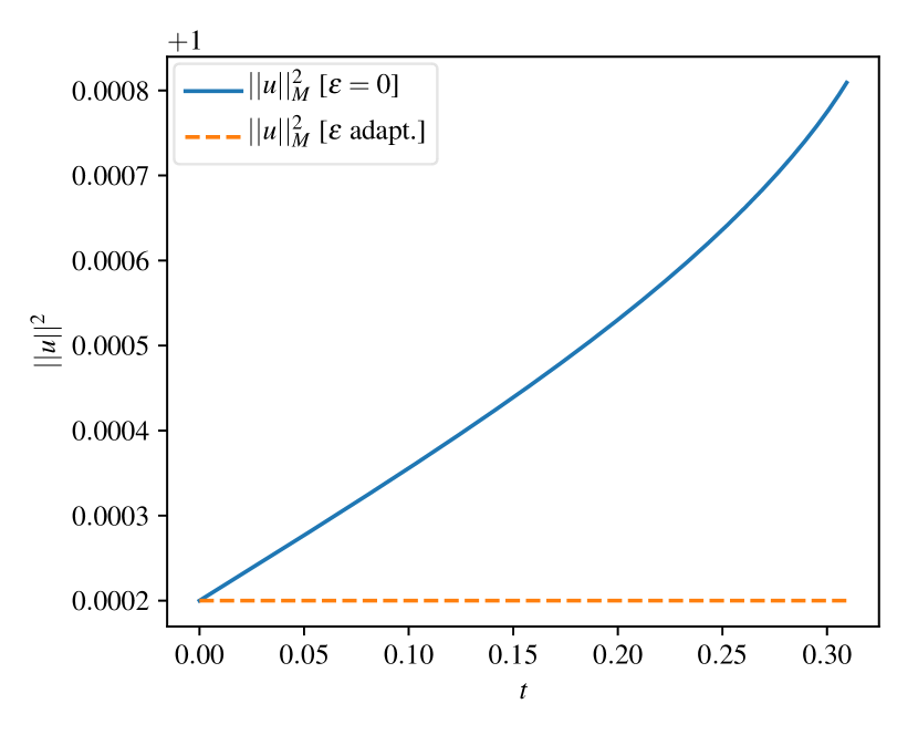
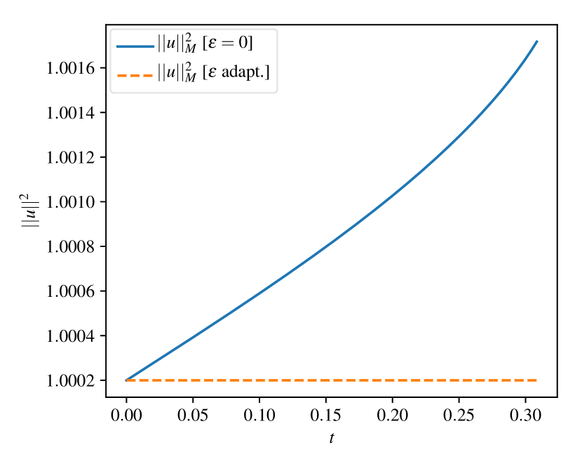
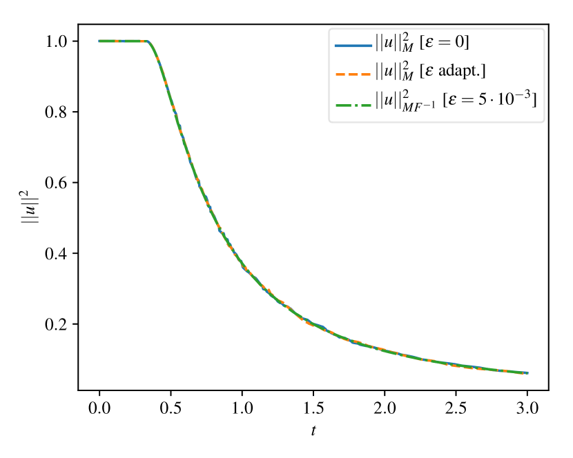
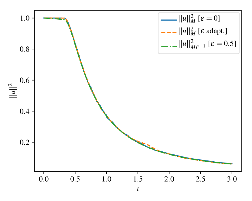
First of all, we note that the energy profiles for artificial dissipation (left, i.e. Figure 3(a) and Figure 3(c)) and for modal filtering (right, i.e. Figure 3(b) and Figure 3(d)) seem indistinguishable the same. This demonstrates again that modal filtering can be seen as the usage of artificial viscosity and vice versa, especially if a similar adaptive strategy is used.
At time , the solution is still smooth. However, the energy in Figure 3(a) and Figure 3(b) increases if no artificial dissipation or modal filter is applied. Contrary, applying adaptive artificial dissipation or modal filtering results in a constant energy. At time , the solution has developed a discontinuity. All three choices of artificial dissipation or modal filtering (we compare no filtering, adaptive filtering, and constant filtering with a fixed strength) yield nearly visually indistinguishable results for the energy profiles in Figures 3(c) and 3(d) due to the dissipative numerical flux.
Finally, we would like to mention that around the discontinuities we still obtain oscillations if the adaptive strategy is applied since the strategy is less dissipative and does not smooth out the oscillations from the semidiscrete setting. As known in the literature, we can cancel out the oscillations for instance by the usage of limiters which are in accordance with the energy (entropy) inequality [9] or just at the final time by some post-processing method. It should also be noted that the adaptive use of artificial viscosity and modal filtering presented here could be used to render shock capturing methods (e.g. [49, 15, 14, 39]) energy dissipative, which themselves are not but might have some other advantages.
4 Comparison Between an Explicit Method with Modal Filtering and the Application of an Implicit Method
Here, we present the main part of this work. It was describe, for instance, in [27] and [28] that explicit time integration methods may produce entropy whereas in implicit methods entropy may be destroyed. This entropy production of explicit methods is always a problem when going over from semidiscrete stability to fully discrete stability. A classical approach is the usage of implicit methods, for example SBP methods in time, which can be written as implicit Runge-Kutta methods [34, 33, 6]. Then, the semidiscrete analysis translates directly to the fully discrete scheme. Unfortunately, this is not the case for explicit methods and in the literature a lot of works can be found which investigate this issue. Here, we demonstrate that with our adaptive technique from section 3, we can mimic implicit schemes by using explicit ones with additional dissipation. As time integration methods we will focus on Euler methods (explicit and implicit). Further, we will only consider modal filtering, since we have the close connection between modal filtering and artificial dissipation.
The explicit Euler method
| (36) |
introduces an erroneous growth of energy of size , whereas the implicit Euler method
| (37) |
yields artificial dissipation of size per time step. Analogously to 3.3, the estimate of the semidiscretisation can be mimicked by filtering with strength
| (38) |
after each time step. Similarly, application of this filter and an additional filter with strength
| (39) |
afterwards yields a filtered explicit Euler method which mimics the dissipation introduced by an implicit Euler method. These estimates are applied to the linear advection equation (31) in with periodic boundary conditions. The initial condition (33) is evolved during the time interval on a grid of elements using polynomials of degree and an upwind numerical flux.
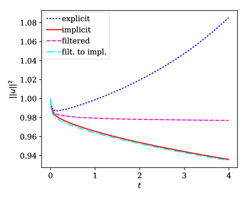
The corresponding energy profiles using time steps are plotted in Figure 4(A) at . The initial condition (33) is also the exact solution of the PDE at , i.e. after two periods. The explicit Euler method (dotted, blue) yields as expected an unconditional energy growths whereas applying adaptive modal filtering once after each time step yields a nearly constant energy. The implicit Euler method (solid red) reduces the energy (introduces artificial dissipation) as can be seen in the figure. However, the estimate of the dissipation introduced by implicit Euler yields an energy result of the explicit Euler method with modal filtering applied twice (dash-dotted, cyan) that is nearly indistinguishable from the implicit one.
Although the estimate of the filter strength is conservative (i.e. only necessary), the energy of the twice filtered explicit solution is slightly less than the energy of the implicitly computed solution. The reason is probably the appearance of some changes of boundary values due to the filtering that triggers additional dissipation by the upwind flux.
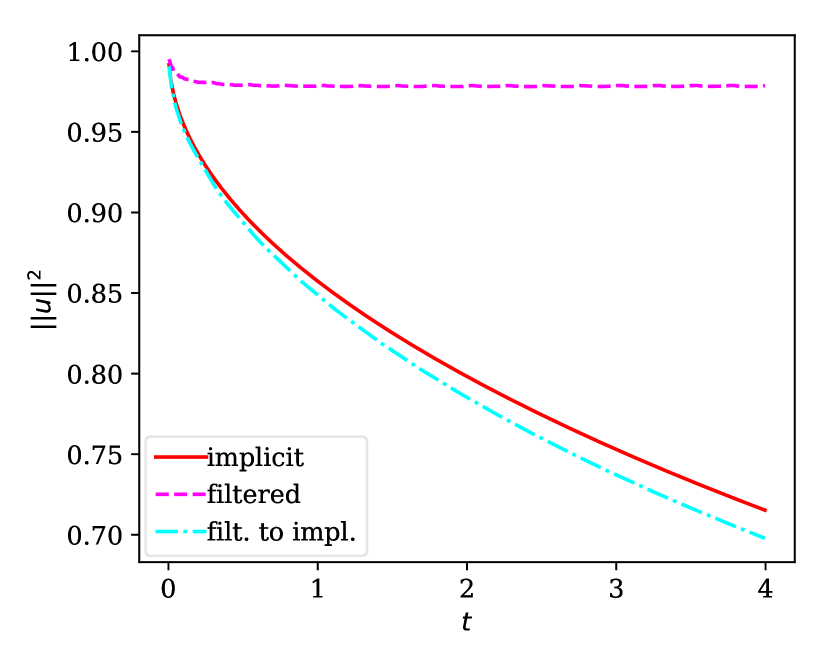
Finally, we note that the same behaviour can be observed if one uses considerably less time steps. In Figure 4(B) the results of the implicit and filtered explicit Euler method using only time steps are plotted. Similarly to the case before, the filtered solutions approximate their targets very well.
5 Summary
The application of SBP operators in time together with a semidiscrete method yields to a fully discrete stable scheme to solve hyperbolic conservation laws as it is done in [32, 33, 12] whereas in [23, 48] a relaxation RK method is applied. Here, we follow another approach and consider also a semidiscretely stable scheme and explicit time integration methods but to reach a fully discrete stable scheme, we apply modal filtering or artificial dissipation, where the strength of dissipation is steered automatically by an adaptive strategy. We consider only the explicit Euler method in this context. However, since strong stability preserving Runge-Kutta schemes can be written as convex combination of explicit Euler steps, our approach can be extended to these methods. Then, we demonstrated by a concrete example that with the usage of modal filters together with our adaptive strategy, we are able to mimic the behavior of an implicit method and can imitate the stability properties of this scheme. This contribution leads to a better understanding of existing algorithms and numerical techniques, especially the application of artificial dissipation as well as modal filtering in the context of numerical methods for hyperbolic conservation laws together with the selection of explicit or implicit time integration methods. A future research topic will be further extension of the study presented here together with implicit SBP operators in time. Also the usage of other adaptive strategies, such as the annihilation of the entropy production in time [27, 28] will be considered.
Appendix
In this section, we show how our analysis from subsection 3.3 can be applied to RK methods and transfer the results to DEC methods, which can be formulated in the RK framework as well. A RK method with stages is given by its Butcher tableau
| (40) |
Here, and . Since there is no explicit dependence on the time in the semidiscretisation, one step from to is given by
| (41) |
Here, the are the stage values of the RK method. It is also possible to express the method via the slopes , as done by [22, Definition II.1.1]. Using the stage values as in (41), we have
| (42) | ||||
where the symmetry of the scalar product has been used in the last step. Here, the first term on the right hand side is consistent with , if the RK method is consistent, i.e. .
The second term of order is undesired. Depending on the method (and the stages, of course), it may be positive or negative. However, if it is positive, then a stability error may be introduced. As a special case, if the method fulfils , this term vanishes. Such methods can conserve quadratic invariants of ordinary differential equations, a topic of geometric numerical integration, see Theorem IV.2.2 of [22], originally proven by [10]. A special kind of these methods are the implicit Gauss methods, see section II.1.3 of [22].
For an explicit method ( for ), the undesired term of order in (42) can be rewritten as
| (43) | ||||
This undesired increase of the norm may be remedied by the application of an adaptive modal filter . Analogously to subsection (3.3), the adaptive filter strength may be estimated via
| (44) | ||||
if the term of order is non-negative. In a modal Legendre basis , the (exact) modal filter is given by (25). Thus,
| (45) |
is required. Here, are the coefficients of the polynomial , expressed in the Legendre basis of polynomials of degree . Following (27), the filter strength can be estimated by
| (46) | ||||
for . Using (since approximates the exact norm on the left hand side), this results in
| (47) |
(47) is the general estimation. We can derive estimation (30) from (47) using the coefficients for the explicit Euler method.
Acknowledgments
Jan Glaubitz was supported by the German Research Foundation (DFG, Deutsche Forschungsgemeinschaft) under Grant SO 363/15-1. Philipp Öffner was supported by SNF project “Solving advection dominated problems with high order schemes with polygonal meshes: application to compressible and incompressible flow problems” and the UZH Postdoc Grant. Hendrik Ranocha was supported by the German Research Foundation (DFG, Deutsche Forschungsgemeinschaft) under Grant SO 363/14-1.
References
- [1] R Abgrall “High order schemes for hyperbolic problems using globally continuous approximation and avoiding mass matrices” In Journal of Scientific Computing 73.2-3 Springer, 2017, pp. 461–494
- [2] Remi Abgrall “A general framework to construct schemes satisfying additional conservation relations. Application to entropy conservative and entropy dissipative schemes” In Journal of Computational Physics 372 Elsevier, 2018, pp. 640–666
- [3] Rémi Abgrall “Some remarks about conservation for residual distribution schemes” In Computational Methods in Applied Mathematics 18.3 De Gruyter, 2018, pp. 327–351
- [4] Remi Abgrall, Elise le Meledo and Phiipp Öffner “On the Connection between Residual Distribution Schemes and Flux Reconstruction” In arXiv preprint arXiv:1807.01261, 2018
- [5] Rémi Abgrall, Philipp Öffner and Hendrik Ranocha “Reinterpretation and Extension of Entropy Correction Terms for Residual Distribution and Discontinuous Galerkin Schemes”, 2019 arXiv:1908.04556 [math.NA]
- [6] Pieter D Boom and David W Zingg “High-order implicit time-marching methods based on generalized summation-by-parts operators” In SIAM Journal on Scientific Computing 37.6 SIAM, 2015, pp. A2682–A2709 DOI: 10.1137/15M1014917
- [7] Claudio Canuto, M Yousuff Hussaini, Alfio Quarteroni and Thomas A Zang “Spectral Methods: Fundamentals in Single Domains” Berlin Heidelberg: Springer, 2006 DOI: 10.1007/978-3-540-30726-6
- [8] Mark H Carpenter, Travis C Fisher, Eric J Nielsen and Steven H Frankel “Entropy Stable Spectral Collocation Schemes for the Navier-Stokes Equations: Discontinuous Interfaces” In SIAM Journal on Scientific Computing 36.5 SIAM, 2014, pp. B835–B867
- [9] Tianheng Chen and Chi-Wang Shu “Entropy stable high order discontinuous Galerkin methods with suitable quadrature rules for hyperbolic conservation laws” In Journal of Computational Physics 345 Elsevier, 2017, pp. 427–461
- [10] GJ Cooper “Stability of Runge-Kutta methods for trajectory problems” In IMA Journal of Numerical Analysis 7.1 Oxford University Press, 1987, pp. 1–13
- [11] Ulrik Skre Fjordholm, Siddhartha Mishra and Eitan Tadmor “Arbitrarily high-order accurate entropy stable essentially nonoscillatory schemes for systems of conservation laws” In SIAM Journal on Numerical Analysis 50.2 SIAM, 2012, pp. 544–573
- [12] Lucas Friedrich et al. “Entropy Stable Space–Time Discontinuous Galerkin Schemes with Summation-by-Parts Property for Hyperbolic Conservation Laws” In Journal of Scientific Computing 80.1 Springer, 2019, pp. 175–222 DOI: 10.1007/s10915-019-00933-2
- [13] Gregor J Gassner, Andrew R Winters and David A Kopriva “A well balanced and entropy conservative discontinuous Galerkin spectral element method for the shallow water equations” In Applied Mathematics and Computation 272 Elsevier, 2016, pp. 291–308
- [14] Jan Glaubitz “Shock capturing by Bernstein polynomials for scalar conservation laws” In Applied Mathematics and Computation 363 Elsevier, 2019, pp. 124593 DOI: 10.1016/j.amc.2019.124593
- [15] Jan Glaubitz and Anne Gelb “High order edge sensors with regularization for enhanced discontinuous Galerkin methods” In SIAM Journal on Scientific Computing 41.2 SIAM, 2019, pp. A1304–A1330 DOI: 10.1137/18M1195280
- [16] Jan Glaubitz et al. “Smooth and compactly supported viscous sub-cell shock capturing for discontinuous Galerkin methods” In Journal of Scientific Computing 79.1 Springer, 2019, pp. 249–272 DOI: 10.1007/s10915-018-0850-3
- [17] Jan Glaubitz, Philipp Öffner and Thomas Sonar “Application of modal filtering to a spectral difference method” In Mathematics of Computation 87.309, 2018, pp. 175–207 DOI: 10.1090/mcom/3257
- [18] David Gottlieb and Jan S Hesthaven “Spectral methods for hyperbolic problems” In Partial Differential Equations Elsevier, 2001, pp. 83–131
- [19] Sigal Gottlieb, David I Ketcheson and Chi-Wang Shu “Strong stability preserving Runge-Kutta and multistep time discretizations” World Scientific, 2011
- [20] Jean-Luc Guermond, Richard Pasquetti and Bojan Popov “Entropy viscosity method for nonlinear conservation laws” In Journal of Computational Physics 230.11 Elsevier, 2011, pp. 4248–4267
- [21] Bertil Gustafsson, Heinz-Otto Kreiss and Joseph Oliger “Time dependent problems and difference methods” John Wiley & Sons, 1995
- [22] Ernst Hairer, Christian Lubich and Gerhard Wanner “Geometric numerical integration: structure-preserving algorithms for ordinary differential equations” Springer Science & Business Media, 2006
- [23] David I Ketcheson “Relaxation Runge–Kutta Methods: Conservation and Stability for Inner-Product Norms” Accepted in SIAM Journal on Numerical Analysis, 2019 arXiv:1905.09847 [math.NA]
- [24] Andreas Klöckner, Tim Warburton and Jan S Hesthaven “Viscous shock capturing in a time-explicit discontinuous Galerkin method” In Mathematical Modelling of Natural Phenomena 6.3 EDP Sciences, 2011, pp. 57–83
- [25] Heinz-Otto Kreiss and Joseph Oliger “Stability of the Fourier method” In SIAM Journal on Numerical Analysis 16.3 SIAM, 1979, pp. 421–433
- [26] Yuan Liu, Chi-Wang Shu and Mengping Zhang “Strong stability preserving property of the deferred correction time discretization” In Journal of Computational Mathematics JSTOR, 2008, pp. 633–656
- [27] Carlos Lozano “Entropy Production by Explicit Runge-Kutta Schemes” In Journal of Scientific Computing 76.1 Springer, 2018, pp. 521–565 DOI: 10.1007/s10915-017-0627-0
- [28] Carlos Lozano “Entropy Production by Implicit Runge–Kutta Schemes” In Journal of Scientific Computing Springer, 2019 DOI: 10.1007/s10915-019-00914-5
- [29] Heping Ma “Chebyshev–Legendre Super Spectral Viscosity Method for Nonlinear Conservation Laws” In SIAM Journal on Numerical Analysis 35.3 SIAM, 1998, pp. 893–908
- [30] Andrew Majda, James McDonough and Stanley Osher “The Fourier method for nonsmooth initial data” In Mathematics of Computation 32.144, 1978, pp. 1041–1081
- [31] Ken Mattsson, Magnus Svärd and Jan Nordström “Stable and accurate artificial dissipation” In Journal of Scientific Computing 21.1 Springer, 2004, pp. 57–79
- [32] Samira Nikkar and Jan Nordström “Fully discrete energy stable high order finite difference methods for hyperbolic problems in deforming domains” In Journal of Computational Physics 291 Elsevier, 2015, pp. 82–98
- [33] Jan Nordström “A roadmap to well posed and stable problems in computational physics” In Journal of Scientific Computing 71.1 Springer, 2017, pp. 365–385
- [34] Jan Nordström and Tomas Lundquist “Summation-by-parts in time” In Journal of Computational Physics 251 Elsevier, 2013, pp. 487–499
- [35] Philipp Öffner “Error boundedness of Correction Procedure via Reconstruction / Flux Reconstruction” Submitted In arXiv preprint arXiv:1806.01575, 2018
- [36] Philipp Öffner, Jan Glaubitz and Hendrik Ranocha “Stability of Correction Procedure via Reconstruction With Summation-by-Parts Operators for Burgers’ Equation Using a Polynomial Chaos Approach” In ESAIM: Mathematical Modelling and Numerical Analysis (ESAIM: M2AN) 52.6 EDP Sciences, 2019, pp. 2215–2245 DOI: 10.1051/m2an/2018072
- [37] Philipp Öffner and Hendrik Ranocha “Error Boundedness of Discontinuous Galerkin Methods with Variable Coefficients” In Journal of Scientific Computing 79.3, 2019, pp. 1572–1607 DOI: 10.1007/s10915-018-00902-1
- [38] Philipp Öffner and Thomas Sonar “Spectral convergence for orthogonal polynomials on triangles” In Numerische Mathematik 124.4 Springer, 2013, pp. 701–721 DOI: 10.1007/s00211-013-0530-z
- [39] Philipp Öffner, Thomas Sonar and Martina Wirz “Detecting strength and location of jump discontinuities in numerical data” In Applied Mathematics 4.12 Scientific Research Publishing, 2013, pp. 1
- [40] Hendrik Ranocha “Generalised Summation-by-Parts Operators and Variable Coefficients” In Journal of Computational Physics 362 Elsevier, 2018, pp. 20–48 DOI: 10.1016/j.jcp.2018.02.021
- [41] Hendrik Ranocha “On Strong Stability of Explicit Runge-Kutta Methods for Nonlinear Semibounded Operators”, 2018 arXiv:1811.11601 [math.NA]
- [42] Hendrik Ranocha “Shallow water equations: Split-form, entropy stable, well-balanced, and positivity preserving numerical methods” In GEM – International Journal on Geomathematics 8.1, 2017, pp. 85–133 DOI: 10.1007/s13137-016-0089-9
- [43] Hendrik Ranocha “Some Notes on Summation by Parts Time Integration Methods” In Results in Applied Mathematics 1 Elsevier, 2019, pp. 100004 DOI: 10.1016/j.rinam.2019.100004
- [44] Hendrik Ranocha, Jan Glaubitz, Philipp Öffner and Thomas Sonar “Stability of artificial dissipation and modal filtering for flux reconstruction schemes using summation-by-parts operators” See also arXiv: 1606.00995 [math.NA] and arXiv: 1606.01056 [math.NA] In Applied Numerical Mathematics 128 Elsevier, 2018, pp. 1–23 DOI: 10.1016/j.apnum.2018.01.019
- [45] Hendrik Ranocha and Philipp Öffner “ Stability of Explicit Runge-Kutta Schemes” In Journal of Scientific Computing 75.2, 2018, pp. 1040–1056 DOI: 10.1007/s10915-017-0595-4
- [46] Hendrik Ranocha, Philipp Öffner and Thomas Sonar “Extended skew-symmetric form for summation-by-parts operators and varying Jacobians” In Journal of Computational Physics 342 Elsevier, 2017, pp. 13–28 DOI: 10.1016/j.jcp.2017.04.044
- [47] Hendrik Ranocha, Philipp Öffner and Thomas Sonar “Summation-by-parts operators for correction procedure via reconstruction” In Journal of Computational Physics 311 Elsevier, 2016, pp. 299–328 DOI: 10.1016/j.jcp.2016.02.009
- [48] Hendrik Ranocha et al. “Relaxation Runge–Kutta Methods: Fully-Discrete Explicit Entropy-Stable Schemes for the Compressible Euler and Navier–Stokes Equations” Accepted in SIAM Journal on Scientific Computing, 2019 arXiv:1905.09129 [math.NA]
- [49] Theresa Scarnati, Anne Gelb and Rodrigo B Platte “Using regularization to improve numerical partial differential equation solvers” In Journal of Scientific Computing 75.1 Springer, 2018, pp. 225–252
- [50] Zheng Sun and Chi-Wang Shu “Stability of the fourth order Runge-Kutta method for time-dependent partial differential equations” In Annals of Mathematical Sciences and Applications 2.2, 2017, pp. 255–284 DOI: 10.4310/AMSA.2017.v2.n2.a3
- [51] Zheng Sun and Chi-Wang Shu “Strong Stability of Explicit Runge–Kutta Time Discretizations” In SIAM Journal on Numerical Analysis 57.3 SIAM, 2019, pp. 1158–1182 DOI: 10.1137/18M122892X
- [52] Eitan Tadmor “Convergence of spectral methods for nonlinear conservation laws” In SIAM Journal on Numerical Analysis 26.1 SIAM, 1989, pp. 30–44
- [53] Eitan Tadmor “Entropy stability theory for difference approximations of nonlinear conservation laws and related time-dependent problems” In Acta Numerica 12 Cambridge University Press, 2003, pp. 451–512
- [54] Eitan Tadmor “The numerical viscosity of entropy stable schemes for systems of conservation laws. I” In Mathematics of Computation 49.179, 1987, pp. 91–103
- [55] John VonNeumann and Robert D Richtmyer “A method for the numerical calculation of hydrodynamic shocks” In Journal of applied physics 21.3 AIP, 1950, pp. 232–237
- [56] Niklas Wintermeyer, Andrew R Winters, Gregor J Gassner and David A Kopriva “An entropy stable nodal discontinuous Galerkin method for the two dimensional shallow water equations on unstructured curvilinear meshes with discontinuous bathymetry” In Journal of Computational Physics 340 Elsevier, 2017, pp. 200–242 DOI: 10.1016/j.jcp.2017.03.036