A Galerkin BEM for high-frequency scattering problems based on frequency dependent changes of variables

Abstract

In this paper we develop a class of efficient Galerkin boundary element methods for the solution of two-dimensional exterior single-scattering problems. Our approach is based upon construction of Galerkin approximation spaces confined to the asymptotic behaviour of the solution through a certain direct sum of appropriate function spaces weighted by the oscillations in the incident field of radiation. Specifically, the function spaces in the illuminated/shadow regions and the shadow boundaries are simply algebraic polynomials whereas those in the transition regions are generated utilizing novel, yet simple, frequency dependent changes of variables perfectly matched with the boundary layers of the amplitude in these regions. While, on the one hand, we rigorously verify for smooth convex obstacles that these methods require only an $\mathcal{O}\left(k^{\epsilon}\right)$ increase in the number of degrees of freedom to maintain any given accuracy independent of frequency, and on the other hand, remaining in the realm of smooth obstacles they are applicable in more general single-scattering configurations. The most distinctive property of our algorithms is their remarkable success in approximating the solution in the shadow region when compared with the algorithms available in the literature.

1 Introduction

High-frequency scattering problems have found and continue to find immense interest in the present day computational science. Indeed, over the course of last two decades, very efficient and effective algorithms have been devised for the numerical solution of scattering problems based on variational [28, 18, 7] and integral equation [13, 5, 34, 10] formulations. In exterior scattering simulations, methods that rest on variational formulations naturally demand the design and implementation of efficient non-reflecting boundary conditions [22, 26, 27] to effectively represent the radiation condition at infinity. On the other hand, solvers based on integral equation formulations (cf. the survey [14]) readily encode the radiation condition into the equation by choosing an outgoing fundamental solution. Moreover, for surface scattering simulations considered in this paper, they enable phase extraction, that takes a particularly simple form in single-scattering configurations, and this turns the problem into the estimation of an amplitude whose oscillations are essentially independent of frequency.

In this paper, we develop a class of efficient Galerkin boundary element methods for the solution of two-dimensional exterior single-scattering problems Our approach is based upon construction of Galerkin approximation spaces confined to the known asymptotic behaviour of the aforementioned amplitude. These spaces are defined as direct sums of appropriate function spaces weighted by the oscillations in the incident field of radiation. Specifically, the function spaces in the illuminated/shadow regions and the shadow boundaries are simply algebraic polynomials whereas those in the transition regions (filling up the remaining parts of the boundary of the scatterer) are generated utilizing novel, yet simple, frequency dependent changes of variables perfectly matched with the boundary layers of the amplitude in these regions. While, on the one hand, we rigorously verify for smooth convex obstacles that these methods require only an $\mathcal{O}\left(k^{\epsilon}\right)$ increase in the number of degrees of freedom to maintain any given accuracy independent of frequency, and on the other hand, remaining in the realm of smooth obstacles they are applicable in more general single-scattering configurations. The most distinctive property of our algorithms is their remarkable success in approximating the solution in the shadow region when compared with the algorithms available in the literature.

Indeed, hybrid integral equation methodologies reinforcing the asymptotic characteristics of the unknown into the solution strategy have now become the usual practice in the field. The first attempt in this direction is due to Nédélec et al. [1, 2] where, considering the impedance boundary condition, an $h$-version boundary element method was utilized in conjunction with the method of stationary phase for the evaluation of highly oscillatory integrals (see [17] for a fast multipole variant, and [24] for a fully discrete three-dimensional version). More relevant to our work is the Nyström method proposed by Bruno et al. [12] for the solution of sound-soft scattering problems in the exterior of smooth convex obstacles. The method therein displays the capability of delivering solutions within any prescribed accuracy in frequency independent computational times. While, in this approach, the boundary layers of the slowly varying amplitude around the shadow boundaries are resolved through a cubic root change of variables, the associated highly oscillatory integrals are evaluated to high order utilizing novel extensions of the method of stationary phase (for a three-dimensional variant of this approach we refer to [11]). The algorithm in [12] has had a great impact in computational scattering community and, following the basic principles therein, a number of alternative single-scattering solvers have been developed. Giladi [25] have used a collocation method that integrates Keller’s geometrical theory of diffraction to account for creeping rays in the shadow region. Huybrechs et al.’s collocation method [29] have utilized the numerical steepest descent method in evaluating highly oscillatory integrals and additional collocation points around shadow boundaries to obtain sparse discretizations. The first rigorous numerical analysis relating to a p-version boundary element implementation of these approaches, due to Domínguez et al. [19], has displayed that an increase of $\mathcal{O}(k^{1/9})$ in the number of degrees of freedom is sufficient to preserve a certain accuracy as $k\to\infty$.

The aforementioned methods remain asymptotic due to approximation of the solution by zero in the deep shadow region. In order to cure this deficiency, we have recently developed frequency-adapted Galerkin boundary element methods [20]. Our approach therein was based on utilization of appropriate integral equation formulations of the scattering problem and design of Galerkin approximation spaces as the direct sum of algebraic or trigonometric polynomials weighted by the oscillations in the incident field of radiation. The number of direct summands, namely $4m$ (one for each of the illuminated and deep shadow regions, and the two shadow boundaries; and $m-1$ for each one of the four transition regions), had to increase as $\mathcal{O}(\log k)$ in order to obtain optimal error bounds. Moreover, from a theoretical perspective, we have rigorously shown that these methods can be tuned to demand an increase of $\mathcal{O}(k^{\epsilon})$ in the number of degrees of freedom to maintain a prescribed accuracy independent of frequency. In connection with smooth convex scatterers, this is the best theoretical result available in the literature.

The new Galerkin boundary element methods we develop in this paper, in contrast, utilize novel frequency dependent changes of variables perfectly matched with the asymptotic behaviour of the solution in the transition regions and thereby eliminate the requirement of increasing the number of direct summands defining the Galerkin approximation spaces with increasing wavenumber $k$. While this clearly displays the ease of implementation of these new schemes when compared with our approach in [20], as we rigorously verify, an increase of $\mathcal{O}(k^{\epsilon})$ is still sufficient to fix the approximation error with increasing $k$ but with savings of $\mathcal{O}(\sqrt{\log k})$ in the necessary number of degrees of freedom. Perhaps more importantly, these new schemes yield significantly superior accuracy in the shadow region as depicted through the numerical tests. This is also true when the results are compared with the recent approach taken by Asheim and Huybrechs [4] wherein more advanced phase extraction techniques (unfortunately not supported by rigorous numerical analysis) based on Melrose-Taylor asymptotics [30] are used.

Parallel with the schemes relating to smooth convex obstacles, Galerkin boundary element methods based on phase extraction have also been developed for half-planes and convex polygons where the number of degrees of freedom is either fixed or must increase in proportion to $\log k$ to fix the error with increasing wavenumber $k$. For an extended review of these procedures, we refer to the survey article [14].

As for multiple scattering problems, we refer to Bruno et al. [9] for an extension of the algorithm in [12] to a finite collection of convex obstacles (see also [21] and [3] for a rigorous analysis of this approach in two- and three-dimensional settings respectively, and Boubendir et al. [8] for the acceleration of this procedure through use of dynamical Krylov subspaces and Kirchhoff approximations), and to Chandler-Wilde et al. [15] for a class of nonconvex polygons.

The paper is organized as follows. In §2, we describe the exterior sound-soft scattering problem along with the relevant integral equations and associated Galerkin formulations. In §3, we introduce the new Galerkin schemes for high-frequency single-scattering problems, and state the associated convergence theorem for smooth convex obstacles which constitutes the main result of the paper. To allow a direct comparison, in the same section, we also present a more general version of our algorithm in [20] along with the corresponding approximation properties. The proof of the main result of the paper is given in §4. Finally, the numerical tests appearing in §5 provide a comparison of our methods developed herein and [20]. Specifically they display that these new schemes 1) attain the same global accuracy with a reduced number of degrees of freedom, 2) provide significantly more accurate solutions in the shadow regions, and 3) are applicable not only for smooth convex obstacles but also in more general single-scattering configurations.

2 The scattering problem and Galerkin formulation

The two-dimensional scattering problem we consider in this manuscript is related with the determination of the scattered field $u$ that satisfies the Helmholtz equation

$$\left(\Delta+k^{2}\right)u=0$$

in the exterior of a smooth compact obstacle $K$, the Sommerfeld radiation condition at infinity that amounts to requiring

$$\lim_{\left|x\right|\to\infty}\left|x\right|^{1/2}\left[\partial_{\left|x\right|}-ik\right]u=0$$

uniformly for all directions $x/\left|x\right|$, and the sound-soft boundary condition

$$u=-u^{\rm inc}$$

for a plane-wave incidence $u^{\rm inc}\left(x\right)=e^{ik\alpha\cdot x}$ with direction $\alpha$ ($\left|\alpha\right|=1$) impinging on $K$.

As is well known, the scattered field $u$ can be reconstructed by means of either the direct or the indirect approach [16]. As in the previous attempts aimed at frequency-independent simulations [12, 25, 29, 19, 20], however, here we favour the former wherein the associated (unknown) surface density is the normal derivative of the total field (known as the surface current in electromagnetism) $\eta=\partial_{\nu}\left(u+u^{\rm inc}\right)$ on $\partial K$. Once $\eta$ is available, the scattered field can be recovered through the single-layer potential

$$u(x)=-\int_{\partial K}\Phi(x,y)\,\eta(y)\,ds(y)$$

where

$$\Phi(x,y)=\dfrac{i}{4}\ H_{0}^{(1)}(k|x-y|)$$

is the fundamental solution of the Helmholtz equation, and $H_{0}^{(1)}$ is the Hankel function of the first kind and order zero.

While the new unknown, namely $\eta$, can be expressed as the unique solution of a variety of integral equations [16, 32] taking the form of an operator equation

$$\mathcal{R}_{k}\,\eta=f_{k}$$ (1)

in $L^{2}\left(\partial K\right)$, the solution of (1) corresponds exactly to that of

$$B_{k}(\mu,\eta)=F_{k}(\mu),\quad\text{for all }\mu\in L^{2}(\partial K),$$ (2)

where the sesquilinear form $B_{k}$ and bounded linear functional $F_{k}$ are defined by

$$B_{k}(\mu,\eta)=\langle\mu,\mathcal{R}_{k}\,\eta\rangle_{L^{2}(\partial K)}\quad\text{and}\quad F_{k}(\mu)=\langle\mu,f_{k}\rangle_{L^{2}(\partial K)}.$$ (3)

Equation (2), in turn, is amenable to a treatment by the Galerkin method wherein one determines the Galerkin solution $\hat{\eta}$ approximating the exact solution $\eta$ in a given finite dimensional Galerkin subspace $\hat{X}_{k}$ requiring that

$$B_{k}(\hat{\mu},\hat{\eta})=F_{k}(\hat{\mu}),\quad\text{for all }\hat{\mu}\in\hat{X}_{k}.$$ (4)

Further, provided the sesquilinear form $B_{k}$ is continuous with a continuity constant $C_{k}$ and strictly coercive with a coercivity constant $c_{k}$ so that

$$\left|B_{k}(\mu,\eta)\right|\leq C_{k}\,\|\mu\|\|\eta\|\qquad\text{and}\qquad\mathcal{R}e\ B_{k}(\mu,\mu)\geq c_{k}\,\|\mu\|^{2}$$

for all $\mu,\eta\in L^{2}(\partial K)$, equation (4) is uniquely solvable and C$\acute{e}$a’s lemma entails

$$\|\eta-\hat{\eta}\|\leq\dfrac{C_{k}}{c_{k}}\inf_{\hat{\mu}\in\hat{X}_{k}}\|\eta-\hat{\mu}\|.$$ (5)

Among the aforementioned integral equations, in this connection, combined field (CFIE) and star-combined (SCIE) integral equations step forward as the continuity and coercivity properties of the associated sesquilinear forms are well-understood. More precisely, the sesquilinear form associated with CFIE is known to be continuous (for $k>0$) and coercive (for $k\gg 1$) for convex domains with piecewise analytic $C^{3}$ boundaries with $C_{k}=\mathcal{O}\left(k^{1/2}\right)$ as $k\to\infty$ and $c_{k}\geq 1/2$ for all sufficiently large $k$ [19, 33] (see also [6] for an extension to non-trapping domains). On the other hand, the sesquilinear form corresponding to SCIE is both continuous and coercive (for $k>0$) for star-shaped Lipschitz domains with $C_{k}=\mathcal{O}\left(k^{1/2}\right)$ as $k\to\infty$ and $c_{k}$ independent of $k$ [32].

3 Galerkin approximation spaces based on frequency dependent changes of variables

The developments in this section are independent of the integral equation used as they relate, specifically, to the construction of Galerkin approximation spaces $\hat{X}_{k}$ whose dimension should increase only as $\log k$ with increasing wave number $k$ to ensure that the relative error

$$\inf_{\hat{\mu}\in\hat{X}_{k}}\dfrac{\|\eta-\hat{\mu}\|}{\|\eta\|}$$

in connection with the infimum on the right-hand side of (5) is independent of $k$.

Considering a smooth convex obstacle $K$ illuminated by a plane-wave $u^{\rm inc}(x)=e^{ik\alpha\cdot x}$, our approach is based on phase extraction

$$\eta\left(x\right)=e^{ik\alpha\cdot x}\,\eta^{\rm slow}\left(x\right),\qquad x\in\partial K,$$

and design of approximation spaces adopted to the asymptotic behavior of the amplitude $\eta^{\rm slow}$ that was initially characterised by Melrose and Taylor [30] around the shadow boundaries which we have later generalized to the entire boundary [21].

Theorem 1.

[21, Corollary 2.1] Let $K\subset\mathbb{R}^{2}$ be a compact, strictly convex set with smooth boundary $\partial K$. Then $\eta^{\rm slow}=\eta^{\rm slow}(x,k)$ belongs to the Hörmander class $S^{1}_{2/3,1/3}\left(\partial K\times\left(0,\infty\right)\right)$ and admits an asymptotic expansion

$$\eta^{\rm slow}(x,k)\sim\sum_{p,q\geq 0}a_{p,q}\left(x,k\right)$$

with

$$a_{p,q}(x,k)=k^{2/3-2p/3-q}\,b_{p,q}(x)\,\Psi^{(p)}(k^{1/3}Z(x))$$

where $b_{p,q}$ and $\Psi$ are complex-valued $C^{\infty}$ functions and $Z$ is a real-valued $C^{\infty}$ function that is positive on the illuminated region $\partial K^{IL}=\{x\in\partial K:\alpha\cdot\nu(x)<0\}$, negative on the shadow region $\partial K^{SR}=\{x\in\partial K:\alpha\cdot\nu(x)>0\}$, and vanishes precisely to the first order on the shadow boundaries $\partial K^{SB}=\{x\in\partial K:\alpha\cdot\nu(x)=0\}$. Moreover, the function $\Psi$ admits the asymptotic expansion

$$\Psi(\tau)\sim\sum_{j=0}^{\infty}c_{j}\tau^{1-3j}\qquad\text{as }\tau\to\infty,$$

and $\Psi$ is rapidly decreasing in the sense of Schwartz as $\tau\to-\infty$.

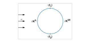
(a) Regions on the unit circle

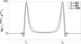
(b) Boundary layers generated

Figure 1: The unit circle illuminated from the left and the associated boundary layers of the solutions.

Theorem 1 clearly displays the challenges associated with the construction of approximation spaces adapted to the asymptotic behavior of $\eta^{\rm slow}$ as it shows that while $\eta^{\rm slow}$ admits a classical asymptotic expansion in the illuminated region and rapidly decays in the shadow region, it possesses boundary layers in the $\mathcal{O}(k^{-1/3})$ neighborhoods of the shadow boundaries (see Fig. 1). We overcome this difficulty by constructing approximation spaces improving upon our approach in [20], and better adapted to the changes in frequency through use of a wavenumber dependent change of variables that resolves the aforementioned boundary layers and that provides a smooth transition from the shadow boundaries into the illuminated and shadow regions. The resulting schemes, when compared with our algorithms in [20], are easier to implement since the Galerkin spaces are represented as the direct sum of a fixed number approximation spaces rather than a number of those that should increase in proportion to $\log k$ as in [20]. Moreover, as we explain, they display better approximation properties from a theoretical perspective since they provide savings on the order of $\sqrt{\log k}$ to attain the same accuracy. Perhaps more importantly, they yield significantly superior accuracy in the shadow region as depicted through the numerical tests.

To describe our approximation spaces, we choose $\gamma$ to be the $L-$periodic arc length parameterization of $\partial K$ in the counterclockwise orientation with $\alpha\cdot\nu\left(\gamma(0)\right)=1$. This ensures that if $0<t_{1}<t_{2}<L$ are the points corresponding to the shadow boundaries

$$\gamma\left(\left\{t_{1},t_{2}\right\}\right)=\partial K^{SB},$$

then the illuminated and shadow regions are given by (see Fig. 1(a))

$$\gamma\left(\left(t_{1},t_{2}\right)\right)=\partial K^{IL}\qquad\text{and}\qquad\gamma\left(\left(t_{2},t_{1}+L\right)\right)=\partial K^{SR}.$$

For $k>1$, we introduce two types of approximation spaces confined to the regions depicted in Figure 2(a)-(b). In both cases, we define the illuminated transition and shadow transition intervals as

$$I_{IT_{1}} =[t_{1}+\xi_{1}k^{-1/3},t_{1}+\xi_{1}^{\prime}]=[a_{1},b_{1}],$$

$$I_{IT_{2}} =[t_{2}-\xi_{2}^{\prime},t_{2}-\xi_{2}k^{-1/3}]=[a_{2},b_{2}],$$

$$I_{ST_{1}} =[t_{1}-\zeta_{1}^{\prime},t_{1}-\zeta_{1}k^{-1/3}]=[a_{3},b_{3}],$$

$$I_{ST_{2}} =[t_{2}+\zeta_{2}k^{-1/3},t_{2}+\zeta_{2}^{\prime}]=[a_{4},b_{4}],$$

and the shadow boundary intervals as

$$I_{SB_{1}} =[t_{1}-\zeta_{1}k^{-1/3},t_{1}+\xi_{1}k^{-1/3}]=[a_{5},b_{5}],$$

$$I_{SB_{2}} =[t_{2}-\xi_{2}k^{-1/3},t_{2}+\zeta_{2}k^{-1/3}]=[a_{6},b_{6}],$$

where the parameters $\xi_{j},\xi_{j}^{\prime},\zeta_{j},\zeta_{j}^{\prime}>0$ ($j=1,2$) are chosen so that

$$t_{1}+\xi_{1}\leq t_{1}+\xi_{1}^{\prime}\overset{(A)}{\leq}t_{2}-\xi_{2}^{\prime}\leq t_{2}-\xi_{2},$$

and

$$t_{2}+\zeta_{2}\leq t_{2}+\zeta_{2}^{\prime}\overset{(B)}{\leq}L+t_{1}-\zeta_{1}^{\prime}\leq L+t_{1}-\zeta_{1}.$$

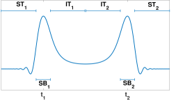
(a) Equalities in (A) and (B)

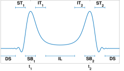
(b) Strict inequalities in (A) and (B)

Figure 2: Regions on the boundary of the unit circle.

Note specifically that the regions in Figure 2(a) correspond to equalities in $(A)$ and $(B)$, and those in Figure 2(b) to strict inequalities. In the latter case, we define the illuminated and deep shadow intervals as

$$I_{IL} =[t_{1}+\xi_{1}^{\prime},t_{2}-\xi_{2}^{\prime}]=[a_{7},b_{7}],$$

$$I_{DS} =[t_{2}+\zeta_{2}^{\prime},L+t_{1}-\zeta_{1}^{\prime}]=[a_{8},b_{8}].$$

With these choices, given $\mathbf{d}=\left(d_{1},\ldots,d_{J}\right)\in\mathbb{Z}_{+}^{J}$ (with $J=6$ and $J=8$ for Figure 2(a) and (b) respectively), we define our $(|\mathbf{d}|+J)-$dimensional Galerkin approximation spaces based on algebraic polynomials and frequency dependent changes of variables as

$$\mathcal{A}_{\mathbf{d}}^{\mathcal{C}}=\bigoplus_{j=1}^{J}\mathds{1}_{\mathcal{I}_{j}}\ e^{ik\,\alpha\cdot\gamma}\ \mathcal{A}_{d_{j}}^{\mathcal{C}}.$$

Here $\mathds{1}_{\mathcal{I}_{j}}$ is the characteristic function of $\mathcal{I}_{j}=[a_{j},b_{j}]$, and

$$\mathcal{A}_{d_{j}}^{\mathcal{C}}=\left\{\begin{array}[]{cl}\mathbb{P}_{d_{j}}\circ\phi^{-1},&\mbox{if }\mathcal{I}_{j}\mbox{ is a transition region},\\[5.0pt] \mathbb{P}_{d_{j}},&\mbox{otherwise},\end{array}\right.$$

where $\mathbb{P}_{d_{j}}$ is the vector space of algebraic polynomials of degree at most $d_{j}$, and $\phi$ is the change of variables on the transition intervals given explicitly as

$$\phi\left(s\right)=\left\{\begin{array}[]{ll}t_{1}+\varphi\left(s\right)k^{\psi\left(s\right)},&s\in I_{IT_{1}},\\[3.00003pt] t_{2}-\varphi\left(s\right)k^{\psi\left(s\right)},&s\in I_{IT_{2}},\\[3.00003pt] t_{1}-\varphi\left(s\right)k^{\psi\left(s\right)},&s\in I_{ST_{1}},\\[3.00003pt] t_{2}+\varphi\left(s\right)k^{\psi\left(s\right)},&s\in I_{ST_{2}},\end{array}\right.$$

wherein $\varphi$ is the affine map

$$\varphi(s)=\left\{\begin{array}[]{ll}\xi_{1}+\left(\xi_{1}^{\prime}-\xi_{1}\right)\dfrac{s-a_{1}}{b_{1}-a_{1}},&s\in I_{IT_{1}},\\[10.00002pt] \xi_{2}^{\prime}+\left(\xi_{2}-\xi_{2}^{\prime}\right)\dfrac{s-a_{2}}{b_{2}-a_{2}},&s\in I_{IT_{2}},\\[10.00002pt] \zeta_{1}^{\prime}+\left(\zeta_{1}-\zeta_{1}^{\prime}\right)\dfrac{s-a_{3}}{b_{3}-a_{3}},&s\in I_{ST_{1}},\\[10.00002pt] \zeta_{2}+\left(\zeta_{2}^{\prime}-\zeta_{2}\right)\dfrac{s-a_{4}}{b_{4}-a_{4}},&s\in I_{ST_{2}},\end{array}\right.$$

and $\psi$ is the linear map

$$\psi(s)=-\dfrac{1}{3}\left\{\begin{array}[]{ll}\dfrac{b_{1}-s}{b_{1}-a_{1}},&s\in I_{IT_{1}},\\[10.00002pt] \dfrac{s-a_{2}}{b_{2}-a_{2}},&s\in I_{IT_{2}},\\[10.00002pt] \dfrac{s-a_{3}}{b_{3}-a_{3}},&s\in I_{ST_{1}},\\[10.00002pt] \dfrac{b_{4}-s}{b_{4}-a_{4}},&s\in I_{ST_{2}}.\end{array}\right.$$

The change of variables $\phi$ is constructed so that, for $j=1,2,3,4$, the map $\phi:[a_{j},b_{j}]\to[a_{j},b_{j}]$ is an orientation preserving diffeomorphism and the exponent $\psi$ of $k$ increases linearly from $-1/3$ to $0$ as we move away from the shadow boundaries into the illuminated or shadow regions. While on the one hand this choice guarantees that the degrees of freedom assigned to the $\mathcal{O}(k^{-1/3})$ neighborhoods of the shadow boundaries remains fixed with increasing wave-number $k$, and on the other hand it also ensures that the approximation spaces are perfectly adapted to the asymptotic behaviour of the solution.

Remark 2.

Note that, by construction, $\gamma(\cup_{j=1}^{J}\mathcal{I}_{j})=\partial K$ and the intervals $\mathcal{I}_{j}$ intersect either trivially or only at an end point. Therefore we can clearly identify $L^{2}\left(\partial K\right)$ and $L^{2}(\cup_{j=1}^{J}\mathcal{I}_{j})$ through the ($L-$periodic arc length) parametrization $\gamma$. This will be the convention we shall follow without any further reference in the rest of the paper.

With the above definitions, the Galerkin formulation of problem (1) is equivalent to finding the unique $\hat{\eta}\in\mathcal{A}_{\mathbf{d}}^{\mathcal{C}}$ such that

$$B_{k}(\hat{\mu},\hat{\eta})=F_{k}(\hat{\mu}),\quad\text{for all }\hat{\mu}\in\mathcal{A}_{\mathbf{d}}^{\mathcal{C}}.$$ (6)

While the following theorem constitutes the main result of the paper and provides the approximation properties of the solution of equation (6), its proof is deferred to the next section. Hereafter we write $A\lesssim_{a,b,\ldots}B$ to mean $0\leq A\leq cB$ for a positive constant $c$ that depends only on $a,b,\ldots$.

Theorem 3.

Given $k_{0}>1$ and $k\geq k_{0}$, suppose that the sesquilinear form $B_{k}$ in (3) associated with the integral operator $\mathcal{R}_{k}$ in (1) is continuous with a continuity constant $C_{k}$ and coercive with a coercivity constant $c_{k}$. Then, for all $n_{j}\in\{0,\ldots,d_{j}+1\}$ $(j=1,\ldots,J)$, we have

$$\|\eta-\hat{\eta}\|_{L^{2}(\partial K)}\lesssim_{n_{1},\ldots,n_{J},k_{0}}\dfrac{C_{k}}{c_{k}}\,k\sum_{j=1}^{J}\dfrac{E(k,j)}{\left(d_{j}\right)^{n_{j}}}$$

for the Galerkin solution $\hat{\eta}$ to (6) where

$$E(k,j)=\left\{\begin{array}[]{ll}\left(\log k\right)^{n_{j}+1/2},&j=1,2,3,4\ (\text{transition regions}),\\[5.0pt] k^{-1/6},&j=5,6\,\qquad(\text{shadow boundaries});\end{array}\right.$$

if $J=8$, then

$$E(k,j)=1,\qquad j=7,8,\quad(\text{illuminated and shadow regions}).$$

Since $\eta$ has the same asymptotic order with $k$ as $k\to\infty$ (see e.g. [30]), if we assign the same polynomial degree to each interval $\mathcal{I}_{j}$, we obtain the following estimate for the relative error.

Corollary 4.

Under the assumptions of Theorem 3, if the same polynomial degree $d=d_{1}=\ldots=d_{J}$ is used on each interval, then for all $n\in\{0,\ldots,d+1\}$, there holds

$$\dfrac{\|\eta-\hat{\eta}\|_{{}_{L^{2}(\partial K)}}}{\|\eta\|_{{}_{L^{2}(\partial K)}}}\lesssim_{n,k_{0}}\dfrac{C_{k}}{c_{k}}\dfrac{\left(\log k\right)^{n+1/2}}{d^{n}}$$ (7)

for the Galerkin solution $\hat{\eta}$ to (6).

Theorem 3 and Corollary 4 display the improved convergence characteristics of the Galerkin approximation spaces based on changes of variables when compared with our approach in [20] wherein we have treated the transition regions in a different way (specifically, rather than utilizing a change of variables, we have divided the transition regions into an optimal number of subregions depending on the underlying frequency and used approximation spaces in the form of the plane-wave weighted by polynomials). Moreover, as will be depicted in the numerical tests, the Galerkin approximation spaces based on changes of variables display a significant improvement over those in [20] in terms of the accuracy of solutions in the shadow regions.

In order to allow for a direct comparison, here we present a more flexible version of our algorithm in [20], that is better suited for different geometries, together with the associated convergence results. To this end, given $m\in\mathbb{N}$, $0\leq\epsilon_{m}<\epsilon_{m-1}<\cdots<\epsilon_{1}<1/3$, and constants $\xi_{1},\xi_{2},\zeta_{1},\zeta_{2}>0$ with $t_{1}-\xi_{1}<t_{2}-\xi_{2}$ and $t_{2}+\zeta_{2}<L+t_{1}-\zeta_{1}$, we define the associated illuminated transition and shadow transition intervals as

$$I_{IT_{1}} =[t_{1}+\xi_{1}k^{-1/3+\epsilon_{m}},t_{1}+\xi_{1}k^{-1/3+\epsilon_{1}}],$$

$$I_{IT_{2}} =[t_{2}-\xi_{2}k^{-1/3+\epsilon_{1}},t_{2}-\xi_{2}k^{-1/3+\epsilon_{m}}],$$

$$I_{ST_{1}} =[t_{1}-\zeta_{1}k^{-1/3+\epsilon_{1}},t_{1}-\zeta_{1}k^{-1/3+\epsilon_{m}}],$$

$$I_{ST_{2}} =[t_{2}+\zeta_{2}k^{-1/3+\epsilon_{m}},t_{2}+\zeta_{2}k^{-1/3+\epsilon_{1}}],$$

and, rather than utilizing a change of variables in the transition intervals, we divide each one into $m-1$ subintervals by setting

$$I_{IT_{1}}^{j} =[t_{1}+\xi_{1}k^{-1/3+\epsilon_{j+1}},t_{1}+\xi_{1}k^{-1/3+\epsilon_{j}}],$$

$$I_{IT_{2}}^{j} =[t_{2}-\xi_{2}k^{-1/3+\epsilon_{j}},t_{2}-\xi_{2}k^{-1/3+\epsilon_{j+1}}],$$

$$I_{ST_{1}}^{j} =[t_{1}-\zeta_{1}k^{-1/3+\epsilon_{j}},t_{1}-\zeta_{1}k^{-1/3+\epsilon_{j+1}}],$$

$$I_{ST_{2}}^{j} =[t_{2}+\zeta_{2}k^{-1/3+\epsilon_{j+1}},t_{2}+\zeta_{2}k^{-1/3+\epsilon_{j}}],$$

for $j=1,\ldots,m-1$. In addition to these $4m-4$ transition intervals, we further define the shadow boundary intervals as

$$I_{SB_{1}} =[t_{1}-\zeta_{1}k^{-1/3+\epsilon_{m}},t_{1}+\xi_{1}k^{-1/3+\epsilon_{m}}],$$

$$I_{SB_{2}} =[t_{2}-\xi_{1}k^{-1/3+\epsilon_{m}},t_{2}+\zeta_{2}k^{-1/3+\epsilon_{m}}],$$

and the illuminated region and shadow region intervals as

$$I_{IL} =[t_{1}+\xi_{1}k^{-1/3+\epsilon_{1}},t_{2}-\xi_{2}k^{-1/3+\epsilon_{1}}],$$

$$I_{DS} =[t_{2}+\zeta_{2}k^{-1/3+\epsilon_{1}},L+t_{1}-\zeta_{1}k^{-1/3+\epsilon_{1}}].$$

These give rise to a total of $4m$ intervals which we shall denote as $\mathcal{I}_{j}$ $(j=1,\ldots,4m)$. Reasoning as before, we identify $L^{2}\left(\partial K\right)$ with $L^{2}(\cup_{j=1}^{4m}\mathcal{I}_{j})$. Given $\mathbf{d}=\left(d_{1},\ldots,d_{4m}\right)\in\mathbb{Z}_{+}^{4m}$, we now define the $(\left|\mathbf{d}\right|+4m)-$dimensional Galerkin approximation space based on algebraic polynomials as

$$\mathcal{A}_{\mathbf{d}}=\bigoplus_{j=1}^{4m}\,\mathds{1}_{\mathcal{I}_{j}}\ e^{ik\,\alpha\cdot\gamma}\ \mathbb{P}_{d_{j}}.$$ (8)

The associated Galerkin formulation of (1) is to find the unique $\hat{\eta}\in\mathcal{A}_{\mathbf{d}}$ such that

$$B_{k}(\hat{\mu},\hat{\eta})=F_{k}(\hat{\mu}),\quad\text{for all }\hat{\mu}\in\mathcal{A}_{\mathbf{d}}.$$ (9)

Incidentally, the Galerkin approximation spaces defined by equation (8) provide a more flexible version of those in [20] since here we allow for different $\xi$ and $\zeta$ values rather than the values $\xi_{1}=\xi_{2}$ and $\zeta_{1}=\zeta_{2}$ we used in [20]. This clearly renders the new approximation spaces better adapted to different geometries.

Theorem 5.

Suppose that $k$ is sufficiently large and the sesquilinear form $B_{k}$ in (3) associated with the integral operator $\mathcal{R}_{k}$ in (1) is continuous with a continuity constant $C_{k}$ and coercive with a coercivity constant $c_{k}$. Then, for all $n_{j}\in\{0,\ldots,d_{j}+1\}$ $(j=1,\ldots,4m)$, we have

$$\|\eta-\hat{\eta}\|_{L^{2}(\partial K)}\lesssim_{n_{1},\ldots,n_{4m}}\dfrac{C_{k}}{c_{k}}\,k\,\sum_{j=1}^{4m}\dfrac{1+E(k,j)}{\left(d_{j}\right)^{n_{j}}}$$

for the Galerkin solution $\hat{\eta}$ to (9) where

$$E(k,j)=\left\{\begin{array}[]{ll}k^{-(1+3\epsilon_{r+1})/2}\left(k^{(\epsilon_{r}-\epsilon_{r+1})/2}\right)^{n_{j}}\!\!\!\!\!,&j=1,\ldots,4m-4,\,\quad(\text{transition regions}),\\[5.0pt] k^{-1/2}\left(k^{\epsilon_{m}}\right)^{n_{j}},&j=4m-3,4m-2,\ (\text{shadow boundaries}),\\[5.0pt] k^{-(1+3\epsilon_{1})/2}\left(k^{(1/3-\epsilon_{1})/2}\right)^{n_{j}},&j=4m-1,4m,\qquad(\text{illuminated \& shadow reg.}).\end{array}\right.$$

The proof of Theorem 5 is similar to that of Theorem $1$ in [20] and is therefore skipped. On the other hand, exactly as Theorem 1 therein implies Corollary 1 in [20], Theorem 5 above yields the following result.

Corollary 6.

Under the assumptions of Theorem 5, if $\epsilon_{j}$ are chosen as

$$\epsilon_{j}=\dfrac{1}{3}\,\dfrac{2m-2j+1}{2m+1},\qquad j=1,\ldots,m,$$

and the same polynomial degree $d=d_{1}=\ldots=d_{4m}$ is used on each interval, then for all $n\in\{0,\ldots,d+1\}$, there holds

$$\dfrac{\|\eta-\hat{\eta}\|_{{}_{L^{2}(\partial K)}}}{\|\eta\|_{{}_{L^{2}(\partial K)}}}\lesssim_{n}\dfrac{C_{k}}{c_{k}}\,m\,\dfrac{1+k^{-\frac{1}{2}}\left(k^{\frac{1}{6m+3}}\right)^{n}}{d^{n}}$$ (10)

for the Galerkin solution $\hat{\eta}$ to (9).

Remark 7.

Note specifically that if $m$ $($and thus the total number of degrees of freedom$)$ increases in parallel with $\log k$, then $k^{\frac{1}{6m+3}}=\exp(\log k/(6m+3))$ is bounded independently of $k$, and the estimate (10) takes on the form

$$\dfrac{\|\eta-\hat{\eta}\|_{{}_{L^{2}(\partial K)}}}{\|\eta\|_{{}_{L^{2}(\partial K)}}}\lesssim_{n}\dfrac{C_{k}}{c_{k}}\,\dfrac{\log k}{d^{n}}.$$

As for the estimate (7) in Corollary 4 relating to the Galerkin schemes based on changes of variables, if the common local polynomial degree $d$ is proportional to $\log k$ $($say $d\approx d_{0}\,\log k$, with $d_{0}$ independent of $k$, so that the total number of degrees of freedom increases as $\log k$$)$, then the estimate in Corollary reduces to

$$\dfrac{\|\eta-\hat{\eta}\|_{{}_{L^{2}(\partial K)}}}{\|\eta\|_{{}_{L^{2}(\partial K)}}}\lesssim_{n,k_{0}}\dfrac{C_{k}}{c_{k}}\,\dfrac{\sqrt{\log k}}{d_{0}^{n}}.$$

This shows that the Galerkin schemes based on change of variables display better approximation properties when compared with the frequency-adapted Galerkin schemes in [20]. Furthermore, since $C_{k}/c_{k}=\mathcal{O}(k^{\delta})$ with $\delta=1/2$ for SCIE and $\delta=1/3$ for CFIE when the obstacle $K$ is strictly convex (see [6]), given $\varepsilon>0$, if $d_{0}$ grows in parallel with $k^{\varepsilon}$, for sufficiently large $n_{0}$, there holds

$$\dfrac{\|\eta-\hat{\eta}\|_{{}_{L^{2}(\partial K)}}}{\|\eta\|_{{}_{L^{2}(\partial K)}}}\lesssim_{n,k_{0}}\dfrac{1}{d_{0}^{n-n_{0}}}$$

for all $n\geq n_{0}$. This shows that, for any $\epsilon>0$, increasing the total number of degrees of freedom associated with the Galerkin schemes based on change of variables as $\mathcal{O}(k^{\epsilon})$ is sufficient to obtain any prescribed accuracy independent of frequency.

4 Error analysis

In this section we present the proof of Theorem 3. In light of inequality (5), it is sufficient to estimate

$$\inf_{\hat{\mu}\in\mathcal{A}_{\mathbf{d}}^{\mathcal{C}}}\|\eta-\hat{\mu}\|_{L^{2}(\partial K)}.$$

To this end, we make use of the following classical result from approximation theory.

Theorem 8 (Best approximation by algebraic polynomials [31]).

Given an interval $\mathcal{I}=(a,b)$ and $n\in\mathbb{Z}_{+}$, introduce the semi–norms $($for suitable $f$$)$ by

$$\left|f\right|_{n,\mathcal{I}}=\left[\int_{a}^{b}\left|D^{n}f(s)\right|^{2}\left(s-a\right)^{n}\left(b-s\right)^{n}ds\right]^{1/2}.$$ (11)

Then, for all $n\in\{0,\ldots,d+1\}$, there holds

$$\inf_{p\in\mathbb{P}_{d}}\|f-p\|\lesssim_{n}\left|f\right|_{n,\mathcal{I}}\,d^{-n}.$$

Use of Theorem 8, in turn, requires the knowledge of derivative estimates of $\eta^{\rm slow}$ which we present next.

Theorem 9.

Given $k_{0}>0$, there holds

$$\left|D_{s}^{n}\eta^{\rm slow}(s,k)\right|\lesssim_{n,k_{0}}k+\sum\limits_{m=4}^{n+2}\left(k^{-1/3}+\left|w(s)\right|\right)^{-m}$$

for all $n\in\mathbb{Z}_{+}$ and all $k\geq k_{0}$. Here $w(s)=(s-t_{1})(t_{2}-s)$.

Proof.

The same estimate is shown to hold for all sufficiently large $k$ in [19]. Since $D_{s}^{n}\eta^{\rm slow}(s,k)$ depends continuously on $s$ and $k$, the result follows. ∎

We continue with the derivation of estimates on the derivatives of the change of variables $\phi$ on the transition interval $\mathcal{I}_{j}$ $(j=1,2,3,4)$.

Proposition 10.

Given $k_{0}>1$, there holds

$$\left|D^{n}_{s}\phi\right|\lesssim_{n,k_{0}}\left(\log k\right)^{n}k^{\psi}\quad\text{on }\mathcal{I}_{j}\quad(j=1,2,3,4),$$

for all $n\in\mathbb{N}$ and all $k\geq k_{0}$.

Proof.

Since the proof is similar for $j=1,2,3,4$, we concentrate on the case $j=1$. Now since $\varphi^{\prime\prime}=\psi^{\prime\prime}=0$, direct computations entail

$$D^{n}_{s}\phi=\sum_{j=0}^{n}\binom{n}{j}\,D^{n-j}_{s}\varphi\ D^{j}_{s}k^{\psi}=\varphi\ D^{n}_{s}k^{\psi}+D^{1}_{s}\varphi\ D^{n-1}_{s}k^{\psi},\qquad n\geq 1,$$ (12)

and

$$D^{n}_{s}k^{\psi}=\left(D^{1}_{s}\psi\right)^{n}\left(\log k\right)^{n}k^{\psi},\qquad n\geq 0.$$ (13)

Using (13) in (12), we obtain

$$D^{n}_{s}\phi=\left(\varphi\ D^{1}_{s}\psi\ \log k+D^{1}_{s}\varphi\right)\left(D^{1}_{s}\psi\right)^{n-1}\left(\log k\right)^{n-1}k^{\psi},\qquad n\geq 1.$$ (14)

Since, for $k\geq k_{0}>1$,

$$\dfrac{1}{\left|b_{1}-a_{1}\right|}=\dfrac{1}{\xi_{1}^{\prime}-\xi_{1}k^{-1/3}}\leq\dfrac{1}{\xi_{1}^{\prime}-\xi_{1}k_{0}^{-1/3}}\lesssim_{k_{0}}1$$

it follows for $s\in\mathcal{I}_{1}=I_{IT_{1}}$ that

$$\left|D^{1}_{s}\psi\right|=\dfrac{1}{3}\,\dfrac{1}{b_{1}-a_{1}}\lesssim_{k_{0}}1\qquad\text{and}\qquad\left|D^{1}_{s}\varphi\right|=\dfrac{\xi_{1}^{\prime}-\xi_{1}}{b_{1}-a_{1}}\lesssim_{k_{0}}1$$

and, clearly, $\xi_{1}\leq\varphi\leq\xi_{1}^{\prime}$. Use of these inequalities in (14) yields the desired result. ∎

Next we combine Theorem 9 and Proposition 10 to derive estimates on the derivatives of the composition $\eta^{\rm slow}\circ\phi$.

Proposition 11.

Given $k_{0}>0$, there holds

$$\left|D_{s}^{n}(\eta^{slow}\circ\phi)\right|\lesssim_{n,k_{0}}k\left(\log k\right)^{n}\quad\text{on }\mathcal{I}_{j}\quad\left(j=1,2,3,4\right),$$

for all $n\in\mathbb{N}$ and all $k\geq k_{0}$.

Proof.

We fix $k\geq k_{0}>1$ and the interval $\mathcal{I}_{j}$ ($j=1,\ldots,4$). Faá Di Bruno’s formula for the derivatives of a composition states

$$D^{n}\left(f\circ g\right)\left(t\right)=\sum_{\left\{m_{\ell}\right\}}(D^{m}f)(g(t))\prod_{\ell=1}^{n}\dfrac{\ell}{m_{\ell}!}\left(\dfrac{D^{\ell}g(t)}{\ell!}\right)^{m_{\ell}}$$

where the summation is over all $m_{\ell}\in\mathbb{Z}_{+}$ with $n=\sum_{\ell=1}^{n}\ell m_{\ell}$; here $m=\sum_{\ell=1}^{n}m_{\ell}$. This yields

$$\left|D^{n}_{s}\left(\eta^{\rm slow}\circ\phi\right)\right|\lesssim_{n}\sum_{\left\{m_{\ell}\right\}}\left|(D^{m}_{s}\eta^{\rm slow})(\phi)\right|\prod_{\ell=1}^{n}\left|D^{\ell}_{s}\phi\right|^{m_{\ell}}$$

so that an appeal to Proposition 10 entails

$$\left|D^{n}_{s}\left(\eta^{\rm slow}\circ\phi\right)\right|\lesssim_{n,k_{0}}\sum_{\left\{m_{\ell}\right\}}\left|(D^{m}_{s}\eta^{\rm slow})(\phi)\right|\prod_{\ell=1}^{n}\left(\left(\log k\right)^{\ell}k^{\psi}\right)^{m_{\ell}}.$$

Since $n=\sum_{\ell=1}^{n}\ell m_{\ell}$ and $m=\sum_{\ell=1}^{n}m_{\ell}$, we therefore obtain

$$\left|D^{n}_{s}\left(\eta^{\rm slow}\circ\phi\right)\right| \lesssim_{n,k_{0}}\left(\log k\right)^{n}\sum_{\left\{m_{\ell}\right\}}\left|(D^{m}_{s}\eta^{\rm slow})(\phi)\right|k^{m\psi}$$

$$\lesssim_{n,k_{0}}\left(\log k\right)^{n}\sum_{m=0}^{n}\left|(D^{m}_{s}\eta^{\rm slow})(\phi)\right|k^{m\psi}.$$

It is hence sufficient to show, for $m\in\mathbb{Z}_{+}$, that

$$\left|(D^{m}_{s}\eta^{\rm slow})(\phi)\right|k^{m\psi}\lesssim_{m,k_{0}}k.$$

To this end, we note that if $0\leq\ell\leq m$, then

$$\left(k^{-1/3}+\left|\omega(\phi)\right|\right)^{-\ell} =\left(k^{-1/3}+\left|\omega(\phi)\right|\right)^{-m}\left(k^{-1/3}+\left|\omega(\phi)\right|\right)^{m-\ell}$$

$$\leq\left(k^{-1/3}+\left|\omega(\phi)\right|\right)^{-m}\left(k_{0}^{-1/3}+L^{2}\right)^{m-\ell}$$

$$\lesssim_{m,k_{0}}\left(k^{-1/3}+\left|\omega(\phi)\right|\right)^{-m}$$

so that an appeal to Theorem 9 yields

$$\left|D_{s}^{m}\eta^{\rm slow}(\phi)\right|k^{m\psi} \lesssim_{m,k_{0}}\left[k+\sum_{\ell=4}^{m+2}\left(k^{-1/3}+\left|\omega(\phi)\right|\right)^{-\ell}\right]k^{m\psi}$$

$$\lesssim_{m,k_{0}}\left[k+\left(k^{-1/3}+\left|\omega(\phi)\right|\right)^{-\left(m+2\right)}\right]k^{m\psi}$$

$$\lesssim_{m,k_{0}}k+\left(\dfrac{k^{\psi}}{k^{-1/3}+\left|\omega(\phi)\right|}\right)^{m}\left(k^{-1/3}+\left|\omega(\phi)\right|\right)^{-2}$$

$$\lesssim_{m,k_{0}}k+\left(\dfrac{k^{\psi}}{\left|\omega(\phi)\right|}\right)^{m}k^{2/3}$$

where, in the third inequality, we used that $\psi\leq 0$. Thus it is now enough to show that the quotient $k^{\psi}/\left|\omega(\phi)\right|$ is bounded by a constant independent of $k$. This estimation is similar on each of the transition intervals $\mathcal{I}_{j}$ ($j=1,2,3,4$) and we focus on $\mathcal{I}_{1}$. Indeed, on $\mathcal{I}_{1}=I_{IT_{1}}$, we have $\phi-t_{1}=\varphi k^{\psi}$, $\varphi\geq\xi_{1}>0$ and $t_{2}-\phi\geq t_{2}-\left(t_{1}+\xi_{1}^{\prime}\right)\geq\xi_{2}^{\prime}>0$ so that

$$\dfrac{k^{\psi}}{\left|\omega(\phi)\right|}=\dfrac{k^{\psi}}{\left(\phi-t_{1}\right)\left(t_{2}-\phi\right)}=\dfrac{k^{\psi}}{\varphi k^{\psi}\left(t_{2}-\phi\right)}\leq\dfrac{1}{\xi_{1}\,\xi_{2}^{\prime}}.$$

This finishes the proof. ∎

Next we estimate the semi-norms (11) for the composition $\eta^{\rm slow}\circ\phi$ on the transition intervals $\mathcal{I}_{j}$ $(j=1,2,3,4)$.

Corollary 12.

On the transition intervals $\mathcal{I}_{j}$ $(j=1,2,3,4)$, given $k_{0}>1$, there holds

$$\left|\eta^{\rm slow}\circ\phi\right|_{n,\mathcal{I}_{j}}\lesssim_{n,k_{0}}k\left(\log k\right)^{n}$$

for all $n\in\mathbb{N}$ and all $k\geq k_{0}$.

Proof.

On account of Proposition 11, we estimate for $j=1,2,3,4$

$$\left|\eta^{\rm slow}\circ\phi\right|^{2}_{n,\mathcal{I}_{j}} =\int_{a_{j}}^{b_{j}}\left|D^{n}_{s}\left(\eta^{\rm slow}\circ\phi\right)(s)\right|^{2}\left(s-a_{j}\right)^{n}\left(b_{j}-s\right)^{n}ds$$

$$\lesssim_{n,k_{0}}k^{2}\left(\log k\right)^{2n}\int_{a_{j}}^{b_{j}}\left(s-a_{j}\right)^{n}\left(b_{j}-s\right)^{n}ds$$

$$\lesssim_{n,k_{0}}k^{2}\left(\log k\right)^{2n}$$

where we used that $0<b_{j}-a_{j}<L$. Thus the result. ∎

We are now ready to prove Theorem 3.

Proof.

(of Theorem 3): While Céa’s lemma (cf. inequality (5)) entails

$$\|\eta-\hat{\eta}\|_{L^{2}\left(\partial K\right)}\leq\dfrac{C_{k}}{c_{k}}\inf_{\hat{\mu}\in\mathcal{A}_{\mathbf{d}}^{\mathcal{C}}}\|\eta-\hat{\mu}\|_{L^{2}\left(\partial K\right)}$$ (15)

for the unique solution $\hat{\eta}$ of the Galerkin formulation (6), as we identify $L^{2}\left(\partial K\right)$ with $L^{2}(\cup_{j=1}^{J}\mathcal{I}_{j})$ through the $L-$periodic arc length parameterization $\gamma$, there holds

$$\|\eta-\hat{\mu}\|_{L^{2}(\partial K)}=\|\eta-\hat{\mu}\|_{L^{2}\left(\cup_{j=1}^{J}\mathcal{I}_{j}\right)}\leq\sum_{j=1}^{J}\|\eta-\hat{\mu}\|_{L^{2}\left(\mathcal{I}_{j}\right)}$$

for any $\hat{\mu}\in\mathcal{A}_{\mathbf{d}}^{\mathcal{C}}$. Accordingly, the very definition of Galerkin approximation spaces $\mathcal{A}_{\mathbf{d}}^{\mathcal{C}}$ entails

$$\inf_{\hat{\mu}\in\mathcal{A}_{\mathbf{d}}^{\mathcal{C}}}\|\eta-\hat{\mu}\|_{L^{2}(\partial K)}\leq\sum_{j=1}^{4}\inf_{p\in\mathbb{P}_{d_{j}}}\|\eta^{\rm slow}-p\circ\phi^{-1}\|_{L^{2}(\mathcal{I}_{j})}+\sum_{j=5}^{J}\inf_{p\in\mathbb{P}_{d_{j}}}\|\eta^{\rm slow}-p\|_{L^{2}(\mathcal{I}_{j})}.$$ (16)

On the other hand, utilizing the change of variables $\phi$ on the transition intervals $\mathcal{I}_{j}$ $(j=1,2,3,4)$, for any $p\in\mathbb{P}_{d_{j}}$, we have

$$\|\eta^{\rm slow}-p\circ\phi^{-1}\|^{2}_{L^{2}(\mathcal{I}_{j})} =\int_{a_{j}}^{b_{j}}\left|\left(\eta^{\rm slow}-p\circ\phi^{-1}\right)(s)\right|^{2}ds$$

$$=\int_{a_{j}}^{b_{j}}\left|\left(\eta^{\rm slow}\circ\phi-p\right)(s)\right|^{2}D^{1}_{s}\phi(s)\,ds$$

$$\lesssim_{k_{0}}\log k\ \|\eta^{\rm slow}\circ\phi-p\|^{2}_{L^{2}(\mathcal{I}_{j})}$$

where we used Proposition 10 in conjunction with the fact that $k^{\psi}<1$. Combining this last estimate with (15) and (16), we deduce

$$\|\eta-\hat{\eta}\|_{L^{2}\left(\partial K\right)}\lesssim_{k_{0}}\dfrac{C_{k}}{c_{k}}\left\{\sum_{j=1}^{4}\left(\log k\right)^{1/2}\inf_{p\in\mathbb{P}_{d_{j}}}\|\eta^{\rm slow}\circ\phi-p\|_{L^{2}(\mathcal{I}_{j})}+\sum_{j=5}^{J}\inf_{p\in\mathbb{P}_{d_{j}}}\|\eta^{\rm slow}-p\|_{L^{2}(\mathcal{I}_{j})}\right\}$$

and this, on account of Theorem 8, implies

$$\|\eta-\hat{\eta}\|_{L^{2}\left(\partial K\right)}\lesssim_{n_{1},\ldots,n_{J},k_{0}}\dfrac{C_{k}}{c_{k}}\left\{\sum_{j=1}^{4}\left(\log k\right)^{1/2}\left|\eta^{\rm slow}\circ\phi\right|_{n_{j},\mathcal{I}_{j}}d_{j}^{-n_{j}}+\sum_{j=5}^{J}\left|\eta^{\rm slow}\right|_{n_{j},\mathcal{I}_{j}}d_{j}^{-n_{j}}\right\}.$$

Therefore, to complete the proof, it suffices to show that

$$\left|\eta^{\rm slow}\circ\phi\right|_{n_{j},\mathcal{I}_{j}}\lesssim_{n_{j},k_{0}}k\left(\log k\right)^{n_{j}},\qquad j=1,2,3,4,$$ (17)

and

$$\left|\eta^{\rm slow}\right|_{n_{j},\mathcal{I}_{j}}\lesssim_{n_{j},k_{0}}k\,k^{-1/6},\qquad j=5,6,$$ (18)

and (if $J=8$)

$$\left|\eta^{\rm slow}\right|_{n_{j},\mathcal{I}_{j}}\lesssim_{n_{j},k_{0}}k,\qquad j=7,8.$$ (19)

While the estimates in (17) are given by Corollary 12, for the shadow boundary intervals $\mathcal{I}_{j}$ ($j=5,6$) we use Theorem 9 to deduce

$$\left|D_{s}^{n_{j}}\eta^{\rm slow}(s,k)\right|\lesssim_{n_{j},k_{0}}k+\sum_{m=4}^{n_{j}+2}\left(k^{-1/3}+\left|w(s)\right|\right)^{-m}\lesssim_{n_{j},k_{0}}k+k^{(n_{j}+2)/3};$$

this implies

$$\left|\eta^{\rm slow}\right|_{n_{j},\mathcal{I}_{j}}^{2} =\int_{a_{j}}^{b_{j}}\left|D^{n_{j}}_{s}\eta^{\rm slow}(s)\right|^{2}\left(s-a_{j}\right)^{n_{j}}\left(b_{j}-s\right)^{n_{j}}ds$$

$$\lesssim_{n_{j},k_{0}}\left(k+k^{(n_{j}+2)/3}\right)^{2}\left(b_{j}-a_{j}\right)^{2n_{j}+1}$$

$$\lesssim_{n_{j},k_{0}}\left(k+k^{(n_{j}+2)/3}\right)^{2}\left(k^{-1/3}\right)^{2n_{j}+1}$$

$$\lesssim_{n_{j},k_{0}}\left(k\,k^{-1/6}\right)^{2}$$

which justifies the estimates in (18). This completes the proof when $J=6$.

When $J=8$, for the illuminated and shadow region intervals $\mathcal{I}_{j}$ ($j=7,8$), we use Theorem 9 to estimate

$$\left|D_{s}^{n_{j}}\eta^{\rm slow}(s,k)\right|\lesssim_{n_{j},k_{0}}k+\sum_{m=4}^{n_{j}+2}\left(k^{-1/3}+\left|w(s)\right|\right)^{-m}\lesssim_{n_{j},k_{0}}k+\sum_{m=4}^{n_{j}+2}\left|w(s)\right|^{-m}\lesssim_{n_{j},k_{0}}k$$

so that

$$\left|\eta^{\rm slow}\right|_{n_{j},\mathcal{I}_{j}}^{2} =\int_{a_{j}}^{b_{j}}\left|D^{n_{j}}_{s}\eta^{\rm slow}(s)\right|^{2}\left(s-a_{j}\right)^{n_{j}}\left(b_{j}-s\right)^{n_{j}}ds$$

$$\lesssim_{n_{j},k_{0}}k^{2}\left(b_{j}-a_{j}\right)^{2n_{j}+1}$$

$$\lesssim_{n_{j},k_{0}}k^{2}$$

which verifies (19). This finishes the proof. ∎

5 Numerical tests

While the earlier algorithms [12, 25, 29, 4, 19] concerning smooth convex obstacles are either not supported with rigorous numerical analysis [12, 25, 29, 4] and/or remain asymptotic [12, 29, 19] as they approximate the solutions by zero in the deep shadow regions, our recent frequency-adapted Galerkin boundary element methods [20] are supported with a fully rigorous analysis and they provide approximations in the deep shadow region. In this section, we therefore present numerical tests exhibiting the performance of Galerkin boundary element methods based on changes of variables developed herein in comparison with those in [20]. Indeed, as the tests demonstrate, the new schemes attain the same numerical accuracy with a reduced number of degrees of freedom and, most strikingly, they provide significantly improved approximations in the shadow regions.

On a related note, just as we have based the frequency-adapted Galerkin boundary element methods in [20] on either algebraic polynomials or trigonometric polynomials, the Galerkin approximation spaces developed herein can also be based on trigonometric polynomials in which case the Galerkin approximation spaces take on the form

$$\mathcal{T}^{\mathcal{C}}_{\mathbf{d}}=\bigoplus_{j=1}^{J}\mathds{1}_{\mathcal{I}_{j}}\ e^{ik\,\alpha\cdot\gamma}\ \mathcal{T}_{d_{j}}^{\mathcal{C}}$$

where each $d_{j}$ is even,

$$\mathcal{T}_{d_{j}}^{\mathcal{C}}=\left\{\begin{array}[]{cl}\mathbb{T}_{d_{j}}(\mathcal{I}_{j})\circ\phi^{-1},&\mbox{if }\mathcal{I}_{j}\mbox{ is a transition region},\\[5.0pt] \mathbb{T}_{d_{j}}(\mathcal{I}_{j}),&\mbox{otherwise},\end{array}\right.$$

and, for a generic interval $\mathcal{I}=[a,b]$ and an even integer $d$, $\mathbb{T}_{d}(\mathcal{I})$ is the space of $(b-a)$-periodic trigonometric polynomials of degree at most $d$ on $\mathcal{I}$. In this section, we also present numerical tests that display the improvements provided by the approximation spaces $\mathcal{T}^{\mathcal{C}}_{\mathbf{d}}$ over their trigonometric counterparts

$$\mathcal{T}_{\mathbf{d}}=\bigoplus_{j=1}^{4m}\mathds{1}_{\mathcal{I}_{j}}\ e^{ik\,\alpha\cdot\gamma}\ \mathbb{T}_{d_{j}}(\mathcal{I}_{j})$$

in [20]. Indeed, as in [20], here the intervals $\mathcal{I}_{j}$ are chosen to overlap with their immediate neighbors but the size of the overlap diminishes as $k\to\infty$. This requirement is related with the need to introduce a smooth partition of unity confined to the various regions on the boundary of the scatterer for both theoretical and practical reasons. For details of this construction, we refer to [20]. Incidentally, the error analysis corresponding to the spaces $\mathcal{T}^{\mathcal{C}}_{\mathbf{d}}$ can be carried out utilizing the techniques in §4 in conjunction with those in [20, §4.2].

An important component of our algorithms relates to the choice of bases for the spaces of algebraic and trigonometric polynomials and, in order to minimize the numerical instabilities arising from the use of high-degree polynomials, on any generic interval $\mathcal{I}=[a,b]$, we use the bases $\{\rho^{r}:r=0,\ldots,d\}$ and $\{(\rho\circ\phi^{-1})^{r}:r=0,\ldots,d\}$ for $\mathbb{P}_{d}$ and $\mathbb{P}_{d}\circ\phi^{-1}$ respectively where $\rho$ is the affine function that maps the interval $\mathcal{I}$ onto $[-1,1]$. Similarly, for even values of $d$, we employ the bases $\{\exp({ir\rho}):r=-\frac{d}{2},\ldots,\frac{d}{2}\}$ and $\{\exp({ir(\rho\circ\phi^{-1}}):r=-\frac{d}{2},\ldots,\frac{d}{2}\}$ for $\mathbb{T}_{d}(\mathcal{I})$ and $\mathbb{T}_{d}\circ\phi^{-1}(\mathcal{I})$ where, this time, $\rho$ maps the interval $\mathcal{I}$ onto $[0,2\pi]$.

In the same vein, the choice of the parameters $\xi,\xi^{\prime},\zeta,\zeta^{\prime}$ appearing in the definitions of the intervals $I_{IT_{j}},I_{ST_{j}},I_{SB_{j}}$ ($j=1,2$) and $I_{IT},I_{DS}$ is of great importance since a random choice may result in a loss of accuracy due to poor resolution of the boundary layers in the solution. We therefore optimize these parameters for a small wave number through a simple iterative procedure, and use these values for all larger wave numbers. For instance, when $J=6$, we take $\xi_{1}^{\prime}=\xi_{2}^{\prime}$, $\zeta_{1}^{\prime}=\zeta_{2}^{\prime}$ and initially require that $\alpha\cdot\gamma(\xi_{1}^{\prime})=-1$ and $\alpha\cdot\gamma(\zeta_{1}^{\prime})=1$. We then take $\xi_{1}$ to be the mid-point between $t_{1}$ and $\xi_{1}^{\prime}$, and change it in small increments until the local error in $IT_{1}\cup SB_{1}$ is minimized. We treat the triplet $(t_{2},\xi_{2},\xi_{2}^{\prime})$ similarly. Finally, we fix $\xi_{1}$ and $\xi_{2}$, and change $\xi_{1}^{\prime}=\xi_{2}^{\prime}$ in small increments until the error in $IL\cup IT_{1}\cup IT_{2}\cup SB_{1}\cup SB_{2}$ is minimized. The optimization of $\zeta$ parameters is realized similarly. The computed values are taken as the initial guess for the next iterate, and the procedure is repeated with smaller increments, with step size half that of the previous one, until the variations in the global error stabilizes. Following the prescriptions in [20, §4.2], then we introduce a smooth partition of unity confined to the regions $I_{IT_{j}},I_{ST_{j}},I_{SB_{j}}$ ($j=1,2$) and $I_{IT},I_{DS}$, and optimize the shapes of hat functions therein using a similar iterative procedure (see the left-most panes in Figures 4–6). For further details, we refer to [23].

As for the choice of the integral equation, as we mentioned, the developments central to this paper are independent of the integral equation used. However, in order to allow a simple performance comparison with the aforementioned algorithms, we base our numerical implementations on the CFIE wherein the integral operator and the right-hand side are given by

$$\mathcal{R}_{k}=\dfrac{1}{2}\,I+\mathcal{D}-ik\mathcal{S}\quad\text{and}\quad f_{k}=\dfrac{\partial u^{\rm inc}}{\partial\nu}-iku^{\rm inc}.$$

Here $\mathcal{S}$ is the acoustic single-layer integral operator and $\mathcal{D}$ is its normal derivative, and they are defined by

$$\mathcal{S}\eta(x)=\int_{\partial K}\Phi(x,y)\,\eta(y)\,ds(y),\qquad x\in\partial K,$$

$$\mathcal{D}\eta(x)=\int_{\partial K}\dfrac{\partial\Phi(x,y)}{\partial\nu(x)}\,\eta(y)\,ds(y),\qquad x\in\partial K,$$

where $\nu(x)$ is the outward unit normal to ${\partial K}$.

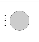
(a) Unit circle: $\alpha=(1,0)$

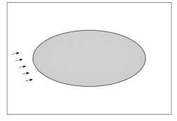
(b) Ellipse: $\alpha=(3,1)/\sqrt{10}$

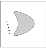
(c) Kite: $\alpha=(4,1)/\sqrt{17}$

Figure 3: Single-scattering geometries and associated incidence directions $\alpha$.

We consider three different single-scattering geometries (see Fig. 3) consisting of the unit circle, the ellipse with major/minor axes (aligned with the $x/y$-axes) of $2/1$, and the kite shaped obstacle given parametrically as $\{(\cos t+0.65\cos 2t-0.65,1.5\sin t)\,:\,t\in[0,2\pi]\}$. The unit circle is the standard example in the aforementioned references since circles are the only two-dimensional obstacles for which explicit solutions are available (through a straightforward Fourier analysis), and thus they allow an unquestionable performance test for single-scattering solvers. As for the ellipse and kite shaped obstacles, we compare the outcome of our numerical implementations with highly accurate reference solutions obtained by a combination of the Nyström and trapezoidal rule discretizations applied to the CFIE [16]. Indeed, the double integrals appearing as the entries of Galerkin matrices are also evaluated utilizing these rules for the inner integrals and the trapezoidal rule for the outer integrals. In order to preserve the high-order approximation properties of these numerical integration rules for smooth and periodic integrands, as in [20], we additionally utilize a smooth partition of unity confined to the regions on the boundary of the scatterer described in Section 3. In each case, based on our experience in [20], the number of discretization points is chosen approximately as $10$ to $12$ points per wave length.

The results of our numerical experiments are presented in the following figures. They are arranged so that the left panes display the support of direct summands forming the associated Galerkin approximation spaces $\mathcal{A}_{\mathbf{d}}$ or $\mathcal{T}_{\mathbf{d}}$ we proposed in [20] or their change of variables counterparts $\mathcal{A}_{\mathbf{d}}^{\mathcal{C}}$ or $\mathcal{T}_{\mathbf{d}}^{\mathcal{C}}$ we developed herein. On the other hand, the middle and right panes depict, respectively, the corrseponding logarithmic relative errors

$$\log_{10}\left(\dfrac{\|\eta-\hat{\eta}\|_{L^{2}(\partial K)}}{\|\eta\|_{L^{2}(\partial K)}}\right)\quad\text{and}\quad\log_{10}\left(\dfrac{\|\eta-\hat{\eta}\|_{L^{2}(\partial K^{SR})}}{\|\eta\|_{L^{2}(\partial K^{SR})}}\right)$$

versus the polynomial degrees used in each subregion (here $\partial K^{SR}=\{x\in\partial K:\alpha\cdot\nu(x)>0\}$ is the shadow region).

Figures 4 and 5 concern convex obstacles (the unit circle and the ellipse), and Figure 6 relates to the non-convex single scattering configuration consisting of the kite. To prevent repetitions, we have chosen to present a comparison of the solutions based on a utilization of the approximation spaces (i) $\mathcal{A}_{\mathbf{d}}$ and $\mathcal{A}_{\mathbf{d}}^{\mathcal{C}}$ for the unit circle in Figure 4, (ii) $\mathcal{T}_{\mathbf{d}}$ and $\mathcal{T}_{\mathbf{d}}^{\mathcal{C}}$ for the ellipse in Figure 5, and (iii) $\mathcal{A}_{\mathbf{d}}^{\mathcal{C}}$ and $\mathcal{T}_{\mathbf{d}}^{\mathcal{C}}$ for the kite in Figure 6.

The first row in Figure 4 displays the results based on an implementation of $\mathcal{A}_{\mathbf{d}}$ with $m=1$ (which corresponds to $8$ direct summands), and the second row to $\mathcal{A}_{\mathbf{d}}^{\mathcal{C}}$ with $J=6$ (giving rise to $6$ direct summands). As is apparent, solutions based on $\mathcal{A}_{\mathbf{d}}^{\mathcal{C}}$ give rise to similar global accuracy as those obtained by $\mathcal{A}_{\mathbf{d}}$ but with a reduction of $\%25$ in the total number of degrees of freedom. Moreover, $\mathcal{A}_{\mathbf{d}}^{\mathcal{C}}$ provides significantly improved accuracies in the shadow region.

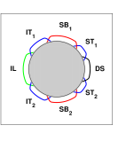
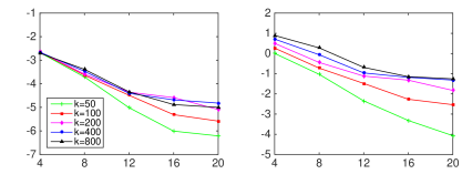
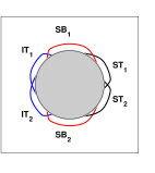
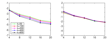
Figure 4: $\mathcal{A}_{\mathbf{d}}$ (first row) vs. $\mathcal{A}_{\mathbf{d}}^{\mathcal{C}}$ (second row) for the unit circle.

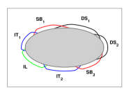
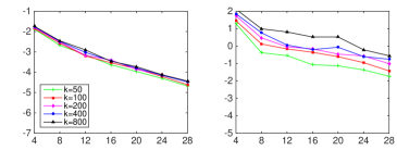
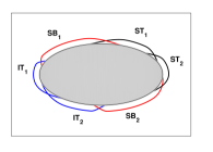
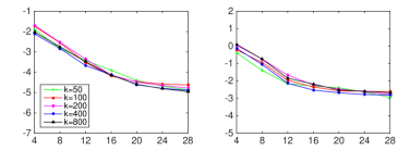
Figure 5: A variant of $\mathcal{T}_{\mathbf{d}}$ (first row) vs. $\mathcal{T}_{\mathbf{d}}^{\mathcal{C}}$ (second row) for the ellipse.

Figure 5 presents the numerical results associated with the ellipse obtained by a variant of the $\mathcal{T}_{\mathbf{d}}$ spaces with $7$ direct summands (see [20] for details) in the first row, and by the $\mathcal{T}_{\mathbf{d}}^{\mathcal{C}}$ spaces with $6$ direct summands ($J=6$) in the second row. In this case, while the $\mathcal{T}_{\mathbf{d}}^{\mathcal{C}}$ spaces provide a slight improvement in the global accuracy over $\mathcal{T}_{\mathbf{d}}$ with savings of about $\%14$ in the total number of degrees of freedom, the approximations they provide in the shadow region are several orders of magnitude better.

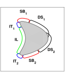
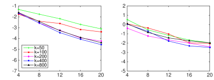
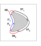
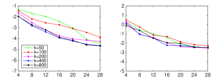
Figure 6: $\mathcal{A}_{\mathbf{d}}^{\mathcal{C}}$ (first row) vs. $\mathcal{T}_{\mathbf{d}}^{\mathcal{C}}$ (second row) for the kite.

Finally, considering the more general single-scattering geometry of the kite, in Figure 6 we present a comparison of the solutions obtained by an implementation of the $\mathcal{A}_{\mathbf{d}}^{\mathcal{C}}$ and $\mathcal{T}_{\mathbf{d}}^{\mathcal{C}}$ spaces. In this case, motivated with our experience in [20] we have constructed $\mathcal{A}_{\mathbf{d}}^{\mathcal{C}}$ spaces based on $7$ direct summands whereas we have used $J=6$ direct summands in forming $\mathcal{T}_{\mathbf{d}}^{\mathcal{C}}$ spaces (see the left-most pane in Fig. 6). As Figure 6 displays, while the algebraic $\mathcal{A}_{\mathbf{d}}^{\mathcal{C}}$ and trigonometric $\mathcal{T}_{\mathbf{d}}^{\mathcal{C}}$ Galerkin approximation spaces based on changes of variables are both well adapted to more general non-convex single-scattering geometries, the latter displays a slightly better performance for higher frequencies in terms of both the global and shadow region errors.

6 Conclusions

In this paper, we proposed a class of Galerkin boundary element methods based on novel changes of variables for the solution of two-dimensional single-scattering problems. The Galerkin approximation spaces, generated in the form of a direct sum of algebraic or trigonometric polynomial spaces weighted by the oscillations in the incident field of radiation, are additionally coupled with novel frequency dependent changes of variables in the transition regions. As we have shown, this construction ensures that the global approximation spaces are perfectly matched with the changes in the boundary layers of the solutions with increasing wave number $k$, and they provide remarkable savings over their counterparts in [20] in regards to the total number of degrees of freedom necessary to obtain a prescribed accuracy. Most notably, the schemes proposed herein display the capability of delivering several orders of magnitude more accurate solutions in the shadow regions.

References

• [1] T. Abboud, J.-C. Nédélec, and B. Zhou. Méthode des équations intégrales pour les hautes fréquences. C. R. Acad. Sci. Paris Sér. I Math., 318(2):165–170, 1994.
• [2] T. Abboud, J.-C. Nédélec, and B. Zhou. Improvements of the integral equation method for high frequency problems. Proceedings of 3rd International Conference on Mathematical Aspects of Wave Propagation Problems, 1995.
• [3] A. Anand, Y. Boubendir, F. Ecevit, and F. Reitich. Analysis of multiple scattering iterations for high-frequency scattering problems. II. The three-dimensional scalar case. Numer. Math., 114(3):373–427, 2010.
• [4] A. Asheim and D. Huybrechs. Extraction of uniformly accurate phase functions across smooth shadow boundaries in high frequency scattering problems. SIAM J. Appl. Math., 74(2):454–476, 2014.
• [5] L. Banjai and W. Hackbusch. Hierarchical matrix techniques for low- and high-frequency Helmholtz problems. IMA J. Numer. Anal., 28(1):46–79, 2008.
• [6] D. Baskin, E. A. Spence, and J. Wunsch. Sharp high-frequency estimates for the Helmholtz equation and applications to boundary integral equations. SIAM J. Math. Anal., 48(1):229–267, 2016.
• [7] D. Boffi. Finite element approximation of eigenvalue problems. Acta Numer., 19:1–120, 2010.
• [8] Y. Boubendir, F. Ecevit, and F. Reitich. Acceleration of an iterative method for the evaluation of high-frequency multiple scattering effects. ArXiv e-prints, May 2016.
• [9] O. Bruno, C. Geuzaine, and F. Reitich. On the o(1) solution of multiple-scattering problems. IEEE Transactions on Magnetics, 41(5):1488–1491, May 2005.
• [10] O. P. Bruno, V. Domínguez, and F.-J. Sayas. Convergence analysis of a high-order Nyström integral-equation method for surface scattering problems. Numer. Math., 124(4):603–645, 2013.
• [11] O. P. Bruno and C. A. Geuzaine. An $O(1)$ integration scheme for three-dimensional surface scattering problems. J. Comput. Appl. Math., 204(2):463–476, 2007.
• [12] O. P. Bruno, C. A. Geuzaine, J. A. Monro, Jr., and F. Reitich. Prescribed error tolerances within fixed computational times for scattering problems of arbitrarily high frequency: the convex case. Philos. Trans. R. Soc. Lond. Ser. A Math. Phys. Eng. Sci., 362(1816):629–645, 2004.
• [13] O. P. Bruno and L. A. Kunyansky. A fast, high-order algorithm for the solution of surface scattering problems: basic implementation, tests, and applications. J. Comput. Phys., 169(1):80–110, 2001.
• [14] S. N. Chandler-Wilde, I. G. Graham, S. Langdon, and E. A. Spence. Numerical-asymptotic boundary integral methods in high-frequency acoustic scattering. Acta Numer., 21:89–305, 2012.
• [15] S. N. Chandler-Wilde, D. P. Hewett, S. Langdon, and A. Twigger. A high frequency boundary element method for scattering by a class of nonconvex obstacles. Numer. Math., 129(4):647–689, 2015.
• [16] D. Colton and R. Kress. Inverse acoustic and electromagnetic scattering theory, volume 93 of Applied Mathematical Sciences. Springer-Verlag, Berlin, 1992.
• [17] E. Darrigrand. Coupling of fast multipole method and microlocal discretization for the 3-D Helmholtz equation. J. Comput. Phys., 181(1):126–154, 2002.
• [18] R. W. Davies, K. Morgan, and O. Hassan. A high order hybrid finite element method applied to the solution of electromagnetic wave scattering problems in the time domain. Comput. Mech., 44(3):321–331, 2009.
• [19] V. Domínguez, I. G. Graham, and V. P. Smyshlyaev. A hybrid numerical-asymptotic boundary integral method for high-frequency acoustic scattering. Numer. Math., 106(3):471–510, 2007.
• [20] F. Ecevit and H. Ç. Özen. Frequency-adapted galerkin boundary element methods for convex scattering problems. Numer. Math., pages 1–45, 2016.
• [21] F. Ecevit and F. Reitich. Analysis of multiple scattering iterations for high-frequency scattering problems. I. The two-dimensional case. Numer. Math., 114(2):271–354, 2009.
• [22] B. Engquist and A. Majda. Absorbing boundary conditions for the numerical simulation of waves. Math. Comp., 31(139):629–651, 1977.
• [23] H. H. Eruslu. An optimal change of variables scheme for single scattering problems. Master’s thesis, Boğaziçi University, Istanbul, 2015.
• [24] M. Ganesh and S. C. Hawkins. A fully discrete Galerkin method for high frequency exterior acoustic scattering in three dimensions. J. Comput. Phys., 230(1):104–125, 2011.
• [25] E. Giladi. Asymptotically derived boundary elements for the Helmholtz equation in high frequencies. J. Comput. Appl. Math., 198(1):52–74, 2007.
• [26] D. Givoli. High-order local non-reflecting boundary conditions: a review. Wave Motion, 39(4):319–326, 2004. New computational methods for wave propagation.
• [27] M. J. Grote and I. Sim. Local nonreflecting boundary condition for time-dependent multiple scattering. J. Comput. Phys., 230(8):3135–3154, 2011.
• [28] J. Hesthaven and T. Warburton. High-order accurate methods for time-domain electromagnetics. CMES-Computer Modeling in Engineering & Sciences, 5(5):395–407, MAY 2004.
• [29] D. Huybrechs and S. Vandewalle. A sparse discretization for integral equation formulations of high frequency scattering problems. SIAM J. Sci. Comput., 29(6):2305–2328, 2007.
• [30] R. B. Melrose and M. E. Taylor. Near peak scattering and the corrected Kirchhoff approximation for a convex obstacle. Adv. in Math., 55(3):242–315, 1985.
• [31] C. Schwab. $p$- and $hp$-finite element methods. Numerical Mathematics and Scientific Computation. The Clarendon Press, Oxford University Press, New York, 1998. Theory and applications in solid and fluid mechanics.
• [32] E. A. Spence, S. N. Chandler-Wilde, I. G. Graham, and V. P. Smyshlyaev. A new frequency-uniform coercive boundary integral equation for acoustic scattering. Comm. Pure Appl. Math., 64(10):1384–1415, 2011.
• [33] E. A. Spence, I. V. Kamotski, and V. P. Smyshlyaev. Coercivity of combined boundary integral equations in high-frequency scattering. Comm. Pure Appl. Math., 68(9):1587–1639, 2015.
• [34] M. S. Tong and W. C. Chew. Multilevel fast multipole acceleration in the Nyström discretization of surface electromagnetic integral equations for composite objects. IEEE Trans. Antennas and Propagation, 58(10):3411–3416, 2010.