Distributed sampled-data control of nonholonomic multi-robot systems with proximity networks

Abstract

This paper considers the distributed sampled-data control problem of a group of mobile robots connected via distance-induced proximity networks. A dwell time is assumed in order to avoid chattering in the neighbor relations that may be caused by abrupt changes of positions when updating information from neighbors. Distributed sampled-data control laws are designed based on nearest neighbor rules, which in conjunction with continuous-time dynamics results in hybrid closed-loop systems. For uniformly and independently initial states, a sufficient condition is provided to guarantee synchronization for the system without leaders. In order to steer all robots to move with the desired orientation and speed, we then introduce a number of leaders into the system, and quantitatively establish the proportion of leaders needed to track either constant or time-varying signals. All these conditions depend only on the neighborhood radius, the maximum initial moving speed and the dwell time, without assuming a prior properties of the neighbor graphs as are used in most of the existing literature.

dcu

,   ,   ,   ,

1 Introduction

Cooperative control of multi-robot/agent systems (MRS/MAS) has generated wide interest for researchers in control and robotics communities. Compared with a single robot, multiple robots can cooperatively accomplish complicated tasks with the advantages of high efficiency and robustness to the link failures. Over the last decade, MRS have wide applications in implementing a large number of tasks ranging from coverage, deployment, rescue, to surveillance and reconnaissance. Among these tasks, a basic one is to reach synchronization, i.e., all robots reach the same state, which actually has close connection with many important engineering applications, such as rendezvous problem [rend, Franices], agreement problem [agree], distributed optimization [oz] and formation control [formation].

Recently, the synchronization problem of MAS has been extensively studied in the literature where the neighbor relations are typically modeled as graphs or networks. For example, Jad and ren, respectively, studied the first-order discrete-time MAS with undirected graphs and directed graphs. murry studied the MAS with first-order continuous-time dynamics. The nonholonomic unicycle MRS are investigated by vision1 and vision2. MAS with nonlinear dynamics, time delays, and measurement noises are also considered [moreau, zhangya, wanglin, litao, shiguodong]. In almost all existing results, the neighbor graphs are required to satisfy certain connectivity assumptions for synchronization. How to verify or guarantee such conditions has been a challenging issue. In order to maintain connectivity of dynamical communication graphs, potential function methods are commonly used when designing the distributed control laws [leader1, diamos, diamos1, connecprev].

For a real world MRS, it is more practical that the dynamics of the system are modeled in a continuous-time manner whereas the control laws are designed based on the sampled-data information. The sampled-data technique is of interest in many situations, such as unreliable information channels, limited bandwidth, transport delay. The synchronization of MAS with sampled-data control laws has been studied [sampling1, sampling2], where the neighbor graphs are also required to satisfy certain connectivity assumptions. It is clear that the potential function techniques are not applicable for the analysis of MAS with continuous-time dynamics and sampled-data control, because connectivity of the networks might be lost between sampling instants. How to analyze the synchronization behavior of such kind of systems becomes more challenging. In this paper, we first present a distributed sampled-data algorithm for a group of nonholonomic unicycle robots with continuous-time dynamics, and provide a comprehensive analysis for the synchronization of the closed-loop hybrid system. In our model, each robot has limited sensing and communication range, and the neighbor relations are described by proximity networks. A dwell time is assumed when updating information from neighbors, implying that the control signals are kept constant between the sampled instants and only updated at discrete-time instants. With such sampled-data information, our design of distributed control laws based on nearest-neighbor rules will clearly result in a hybrid closed-loop system, which is different from the case of discrete-time MAS studied by tang2 and Auto, and is also different from the previous results given by ifac where the control law for the rotational speed is designed using the continuous-time information.

For a multi-agent system, we may design a distributed algorithm to guarantee synchronization of the system, but the synchronization state is inherently determined by the initial states and model parameters. In many practical applications, we expect that the system achieves a desired synchronization state and we can treat that state as a reference signal. The agents that have access to the reference signal are referred to as leaders, and they can help steer the MRS to the desired state. Although a large number of theoretical analysis and results for the leader-follower model have been provided, further theoretical investigation is still needed due to some limitations in the existing theory: i) Similar to the leaderless case, the neighbor graphs are required to be connected or contain spanning trees to guarantee that the followers track the reference signal [Jad, diamos1, toven, renwei2], but there are few results to address how to verify such conditions. ii) In order to guide all agents to accomplish complicated tasks, such as tracking time-varying signals and the containment control problem, a number of (not only one) leaders need to be introduced into the system [renwei2, nature, leaders1, leaders2]. However, quantitative theoretical results for the number of leaders needed are still lack. Hence, this paper considers also a multi-unicycle system with multiple leaders and presents some new quantitative results. The sampled-data information is used to design the control laws for the followers and leaders. For the case of the constant reference signal, we analyze the MRS with heterogeneous agents where the leaders and followers have different dynamics since the reference signal is only obtained by the leaders, and quantitatively provide the proportion of leaders needed to track the reference signal. In addition, we investigate the case where the reference signal is dynamic but piecewise constant, and provide quantitative results for the proportion of leaders needed to track a slowly time-varying signal by analyzing the hybrid dynamics at each stage.

The main contributions of this paper are summarized into the following three aspects. (i) For the leaderless case, we establish a sufficient condition, imposed on the neighborhood radius, the dwell time and the maximum moving speed, to guarantee synchronization of the nonholonomic unicycles, which overcomes the difficulty of requiring a prior connectivity assumption on neighbor graphs used in most of the existing results. (ii) For the leader-follower model, we provide the proportion of leaders needed to guide all robots to track a reference signal which can be constant or slowly time-varying. These quantitative results illustrate that adding leaders is a feasible approach to guide MRS to accomplish some complicated tasks. (iii) For both the leaderless case and leader-following case, we provide comprehensive analysis for nonlinear hybrid closed-loop systems. Different from the work of tang2 and Auto, we need to estimate the synchronization rate of the continuous-time variables (i.e., speed and orientation). Here the speed and orientation are determined by the corresponding values at sampling time instants and they are updated according to the states of relevant neighbors, and the neighbors are defined via the positions of all robots. Hence, the positions, orientations and moving speeds of all robots are coupled. We deal with the coupled relationships by combining the dynamical trajectories of the robots at discrete-time instants with the analysis of continuous-time dynamics in sampling intervals.

The rest of this paper is organized as follows. In Section 2, we present the problem formulation for a leaderless model and provide the main result for synchronization. In Section 3, we first investigate the leader-following problem where the leaders have constant reference signal, and quantitatively provide the ratio of the number of leaders to the number of followers needed to track the signal. We then extend our result to the dynamical tracking where the leaders have time-varying reference signal, and present some simulations to illustrate our theoretical results. Concluding remarks are presented in Section 4.

Notations: For a vector $x\in\mathbb{R}^{m}$, $x^{\prime}$ denotes the transpose of $x$, and $\|x\|$ denotes the 2-norm, i.e., $\|x\|=(x^{\prime}x)^{1/2}$. For a square matrix $A=(a_{ij})_{n\times n}$, $\|A\|$ denotes the 2-norm of $A$, i.e., $\|A\|=\sqrt{\lambda_{\max}AA^{\prime}}$. For any two positive sequences $\{a_{n},n\geq 1\}$ and $\{b_{n},n\geq 1\}$, $a_{n}=O(b_{n})$ means that there exists a positive constant $C$ independent of $n$, such that $a_{n}\leq Cb_{n}$ for any $n\geq 1$; $a_{n}=o(b_{n})$ (or ($a_{n}\ll b_{n}$)) means that $\lim_{n\rightarrow\infty}\frac{a_{n}}{b_{n}}=0$; $a_{n}=\Theta(b_{n})$, if there exist two positive constants $C_{1}$ and $C_{2}$, such that $C_{1}b_{n}\leq a_{n}\leq C_{2}b_{n}$.

2 Leaderless Synchronization

2.1 Problem Formulation

Consider a group of $n$ unicycle robots (or agents) moving in a plane. For a robot $i$ $(i=1,2\cdots,n)$, the position of its center at time $t$ $(t\geq 0)$ is denoted by $X_{i}(t)=(x_{i}(t),y_{i}(t))^{\prime}\in\mathbb{R}^{2}$. The orientation and moving speed of each robot are affected by the states of its local neighbors. The pair of two robots is said to be neighbors if their Euclidean distance is less than a pre-defined radius $r_{n}$. We use $\mathcal{N}_{i}(t)$ to denote the set of the robot $i$’s neighbors at time $t$, i.e.,

$$\mathcal{N}_{i}(t)=\left\{j:\Delta_{ij}(t)<r_{n}\right\},$$ (1)

where $\Delta_{ij}(t)=\|X_{i}(t)-X_{j}(t)\|$ is the Euclidean distance between robots $i$ and $j$. The cardinality of the set $\mathcal{N}_{i}(t)$, i.e., the degree of the agent $i$, is denoted as $d_{i}(t)$. When the robots move in the plane, the neighbor relations dynamically change over time. We use graph $G_{t}=\{V,E_{t}\}$ to describe the relationship between neighbors at time $t$, where the vertex set $V=\{1,2,\cdots,n\}$ is composed of all robots, and the edge set is defined as $E_{t}=\{(i,j)\in V\times V:\Delta_{ij}(t)<r_{n}\}$. The neighbor graphs are distance-induced, and also called geometric graphs or proximity networks.

Let $\theta_{i}(t)$ and $v_{i}(t)$ denote the moving orientation and translational speed of the $i$th robot at time $t$. The dynamics of the robots with nonholonomic constraint for pure rolling and nonslipping is described by the following differential equations (for $i\in V$),

$$\left\{\begin{array}[]{ll}\dot{x}_{i}(t)=v_{i}(t)\cos\theta_{i}(t),&\hbox{}\\ \dot{y}_{i}(t)=v_{i}(t)\sin\theta_{i}(t),&\hbox{}\\ \dot{\theta}_{i}(t)=\omega_{i}(t),&\hbox{}\\ \dot{v}_{i}(t)=u_{i}(t),&\hbox{}\end{array}\right.$$ (6)

where $u_{i}(t)$ and $\omega_{i}(t)$ denote the acceleration and rotational speed of the robot $i$ at time $t$. For robot $i$, what we can control is its rotational speed $\omega_{i}(t)$ and its acceleration $u_{i}(t)$, which is an extension from the standard unicycle model where one controls the translational speed directly. We however need to point out that with this simplified extension physical forces affecting the angular motion, such as side-slip forces and friction forces, are ignored.

For the feasibility of information processing by the robots, we assume that the robots can only receive information and design the control law at discrete-time instants $t_{0}(=0),t_{1},t_{2},\cdots$. To simplify the analysis, we suppose that the dwell time is the same and denoted by $\tau_{n}$, i.e., $t_{k+1}-t_{k}=\tau_{n},k=0,1,\cdots$. At discrete-time instant $t_{k}$, each agent is assumed to sense the relative speed and the relative orientation of its neighbors. That is, for robot $i$, it receives the following sampled-data information at time $t_{k}$, $\left\{v_{j}(t_{k})-v_{i}(t_{k}),\ \theta_{j}(t_{k})-\theta_{i}(t_{k}),\ j\in\mathcal{N}_{i}(t_{k})\right\}.$

Remark 1.

From (1), we see that the neighbor set $\mathcal{N}_{i}(t)$ is determined by the positions of all agents, so it is a continuous-time variable. The neighbor relations might change abruptly when all robots are in motion. The introduction of the dwell time avoids introducing chattering in the abrupt changes caused by the evolution of positions.

Remark 2.

For an agent, the relative positions of its neighbors can be measured by e.g., the geolocation and positioning technologies. Using the position information and the orientation information of the agents, the relative speed at the sampling instants can be calculated. Moreover, the relative speed can also be estimated through observer-based methods by introducing reference robots, which is a different framework and falls into our future research. For the sake of simplicity, we assume that each agent can receive the relative speed of its neighbors in this paper.

The objective of this section is to design the distributed control law for the nonholonomic multi-robot system (6) based on the sampled-data information, such that the closed-loop system becomes synchronized in both orientation and moving speed. Here by synchronization we mean that there exists a common vector $(v,\theta)$, such that for all $i\in V$, we have $\lim_{t\rightarrow\infty}v_{i}(t)=v$ and $\lim_{t\rightarrow\infty}\theta_{i}(t)=\theta.$

For robot $i$, we design the distributed control law according to the widely used nearest-neighbor rule for $t\in[t_{k},t_{k+1})$ ($k=0,1,\cdots$),

$$\left\{\begin{array}[]{ll}u_{i}(t)=\frac{1}{\tau_{n}d_{i}(t_{k})}\sum_{j\in\mathcal{N}_{i}(t_{k})}(v_{j}(t_{k})-v_{i}(t_{k})),&\hbox{}\\ \omega_{i}(t)=\frac{1}{\tau_{n}d_{i}(t_{k})}\sum_{j\in\mathcal{N}_{i}(t_{k})}(\theta_{j}(t_{k})-\theta_{i}(t_{k})),&\hbox{}\end{array}\right.$$ (9)

where $d_{i}(t_{k})$ is the degree of robot $i$ at discrete-time $t_{k}$. Substituting (9) into (6), we obtain the following hybrid closed-loop dynamical system:

$$\left\{\begin{array}[]{ll}\dot{x}_{i}(t)=v_{i}(t)\cos\theta_{i}(t),&\hbox{}\\ \dot{y}_{i}(t)=v_{i}(t)\sin\theta_{i}(t),&\hbox{}\\ \dot{\theta}_{i}(t)=\frac{1}{\tau_{n}d_{i}(t_{k})}\sum_{j\in\mathcal{N}_{i}(t_{k})}(\theta_{j}(t_{k})-\theta_{i}(t_{k})),&\hbox{}\\ \dot{v}_{i}(t)=\frac{1}{\tau_{n}d_{i}(t_{k})}\sum_{j\in\mathcal{N}_{i}(t_{k})}(v_{j}(t_{k})-v_{i}(t_{k})).&\hbox{}\\ \end{array}\right.$$ (14)

Thus, we have for $t\in[t_{k},t_{k+1}]$,

$$\theta_{i}(t)=\left(1-\frac{t-t_{k}}{\tau_{n}}\right)\theta_{i}(t_{k})+\frac{t-t_{k}}{\tau_{n}d_{i}(t_{k})}\sum_{j\in\mathcal{N}_{i}(t_{k})}\theta_{j}(t_{k}),\quad$$ (15)

$$v_{i}(t)=\left(1-\frac{t-t_{k}}{\tau_{n}}\right)v_{i}(t_{k})+\frac{t-t_{k}}{\tau_{n}d_{i}(t_{k})}\sum_{j\in\mathcal{N}_{i}(t_{k})}v_{j}(t_{k}).\quad$$ (16)

In particular, at discrete-time instant $t=t_{k+1}$, the orientation and moving speed evolve according to the following equations:

$$\theta_{i}(t_{k+1})=\frac{1}{d_{i}(t_{k})}\sum_{j\in\mathcal{N}_{i}(t_{k})}\theta_{j}(t_{k}),$$ (17)

$$v_{i}(t_{k+1})=\frac{1}{d_{i}(t_{k})}\sum_{j\in\mathcal{N}_{i}(t_{k})}v_{j}(t_{k}).$$ (18)

In order to investigate the synchronization behavior of the hybrid closed-loop system (14), we need to analyze the discrete-time system at sampling time instants and the continuous-time system in the sampling intervals simultaneously. For the discrete-time system (17) and (18), the algebraic properties of neighbor graphs play a key role. Denote the Laplacian matrix of the graph $G_{t}$ as $L(t)$. The normalized Laplacian matrix is defined as $\mathcal{L}(t)=T^{-1/2}(t)L(t)T^{-1/2}(t)$, where the degree matrix is defined as $T(t)=\hbox{diag}(d_{1}(t),d_{2}(t),\cdots,d_{n}(t))$. The matrix $\mathcal{L}(t)$ is non-negative definite, and 0 is one of the eigenvalues. Thus, we can arrange the eigenvalues of $\mathcal{L}(t)$ according to such a non-decreasing manner $0=\lambda_{0}(t)\leq\lambda_{1}(t)\leq\cdots\leq\lambda_{n-1}(t)$. The spectral gap of graph $G_{t}$ is defined as $\overline{\lambda}(t)=\max\{|1-\lambda_{1}(t)|,|1-\lambda_{n-1}(t)|\}.$

Note that the dynamical behavior of all agents is determined by the configuration formed by the initial states of the agents and model parameters including neighborhood radius, the initial speed and dwell time. It is clear that there are numerous possibilities for the initial configuration of the agents. If we do not impose any assumption on the initial states of the agents, then we can only carry out our analysis based on the worst case and the corresponding results are considerably conservative. To solve this issue, we introduce the following random framework, which accounts for a natural setting on the initial states of all robots. In this section, we consider the synchronization problem of the closed-loop system (14) under the following assumption, and aim to establish synchronization conditions without relying on the dynamical properties of neighbor graphs as are used in most literature.

Assumption 3.

1) The positions, orientations and speeds of all robots at the initial time instant are mutually independent; 2) For all robots, the initial positions are uniformly and independently distributed (u.i.d.) in the (normalized) unit square $[0,1]^{2}$; The initial headings are u.i.d. in $[-\pi,\pi)$; The initial speeds are u.i.d. in the interval $[0,v_{n}]$.

Remark 4.

Under Assumption 3, the initial neighbor graph is called a random geometric graph (RGG), whose properties are well investigated by geometric. However, from (14), the independency between positions of all agents will be destroyed for $t=t_{1},t_{2},\cdots$. Thus, the properties concerning the connectivity of static RGG can not be used.

Remark 5.

Denote the sample spaces of the position, orientation and speed as $\Omega_{1}=[0,1]^{2}$, $\Omega_{2}=[-\pi,\pi]$ and $\Omega_{3}=[0,v_{n}]$. By Assumption 3, our synchronization problem is discussed on the sample space $\Omega=\underbrace{(\Omega_{1}\times\cdots\Omega_{1})}_{n}\times\underbrace{(\Omega_{2}\times\cdots\Omega_{2})}_{n}\times\underbrace{(\Omega_{3}\times\cdots\Omega_{3})}_{n}$, where $\times$ denotes the Cartesian product.

Divide the unit square $[0,1]^{2}$ into $M_{n}$ equally small squares labeled as $1,2,\cdots,M_{n}$, where $M_{n}=\lceil\frac{1}{a_{n}}\rceil^{2}$ with $a_{n}$ satisfying $\sqrt{\log n/n}\ll a_{n}\ll 1$. Denote $N_{k}$ $(1\leq k\leq M_{n})$ as the number of agents in the corresponding small square. Introduce the sets

$$B_{n}=\{\omega:\max_{1\leq j\leq M_{n}}N_{j}=na_{n}^{2}(1+o(1))\},$$ (19)

$$\Theta_{n}=\big{\{}\omega:\max_{i\in V}\big{|}\sum_{j\in\mathcal{N}_{i}(0)}\theta_{j}(0)\big{|}=O(f_{n})\big{\}},$$ (20)

$$\Gamma_{n}=\big{\{}\omega:\max_{i\in V}\big{|}\sum_{j\in\mathcal{N}_{i}(0)}(v_{j}(0)-\frac{v_{n}}{2})\big{|}=O(v_{n}f_{n})\big{\}},$$ (21)

where $f_{n}=\sqrt{nr_{n}^{2}\log n}$. Using Lemma 7 given by Auto, the event $B_{n}$ happens with the probability $\mathbb{P}(B_{n})=1$ for large $n$, where $\mathbb{P}(\cdot)$ denotes the probability of an event. By Assumption 3 and the methods used in Lemma 9 given by Auto, for large $n$, $\mathbb{P}\left(\Theta_{n}\big{|}B_{n}\right)=1$ and $\mathbb{P}\left(\Gamma_{n}\big{|}B_{n}\right)=1$ hold true. Furthermore, by the independency of the orientations and moving speeds for the given agents, it is clear that for large $n$, $\mathbb{P}\left(\Theta_{n}\bigcap\Gamma_{n}\bigcap B_{n}\right)=1$. In the following, we will investigate the dynamical behavior of all agents on the set $\Theta_{n}\bigcap\Gamma_{n}\bigcap B_{n}$, and we omit the words “almost surely” (a.s.) for simplicity. Under the condition that the neighborhood radius satisfies $\sqrt[6]{\log n/n}\ll r_{n}\ll 1$, the maximum and minimum initial degrees satisfy the following equalities

$$d_{\max}=n\pi r_{n}^{2}(1+o(1));\ d_{min}(0)=\frac{n\pi r_{n}^{2}}{4}(1+o(1)).$$ (22)

In fact, for the case where the neighborhood radius independent of $n$, the degrees of the agents can also be estimated by similar methods. The detailed analysis for the estimation of the initial degrees can be found in Theorem 2 given by tang2 for details.

2.2 Main Results

We rewrite the orientation and speed update equations (15) and (16) into the following matrix form for $t\in[t_{k},t_{k+1}]$,

$$\theta(t)=\left(1-\frac{t-t_{k}}{\tau_{n}}\right)\theta(t_{k})+\frac{t-t_{k}}{\tau_{n}}P(t_{k})\theta(t_{k}),$$ (23)

$$v(t)=\left(1-\frac{t-t_{k}}{\tau_{n}}\right)v(t_{k})+\frac{t-t_{k}}{\tau_{n}}P(t_{k})v(t_{k}).$$ (24)

Correspondingly, the equations (17) and (18) are rewritten into the following form,

$$\theta(t_{k+1})=P(t_{k})\theta(t_{k}),$$ (25)

$$v(t_{k+1})=P(t_{k})v(t_{k}),$$ (26)

where the average matrix $P(t_{k})=(p_{ij}(t_{k}))$ is defined as: $p_{ij}(t_{k})=\frac{1}{d_{i}(t_{k})}$ if $(i,j)\in E_{t_{k}}$, and $p_{ij}(t_{k})=0$ otherwise.

A known result for synchronization of the system (25) and (26) can be stated as follows. If the neighbor graphs $G(t_{k})\ (k\geq 0)$ are connected, then all agents move with the same orientation and with the same speed eventually (cf., Jad). The synchronization condition of the system (25) and (26) is imposed on the dynamical properties of neighbor graphs. However, for the system under consideration, the neighbor graphs are defined via the positions of all agents. A comprehensive analysis for the system (14) should include how the change of the positions of all robots affects the dynamical properties of neighbor graphs, which brings challenges for our investigation.

Intuitively, for uniformly distributed agents, if the two agents are not neighbors at the initial time instant, then they are still not neighbors with high probability as the system evolves. That is, if the initial neighbor graph is disconnected, then it is hard to obtain the connectivity of graph $G(t_{k})$ for $k\geq 1$. In order to reach synchronization, the connectivity of the initial neighbor graphs is needed. When the population size of the agents increases, the number of neighbors of each agent will also increase. Thus, the interaction radius can be allowed to decay with the number of agents to guarantee connectivity of the initial neighbor graph. The properties of such graphs have been widely investigated in the fields of wireless sensor networks and random geometric graphs (cf., kumar, geometric). Moreover, the change of neighbor graphs at the time instants $t_{k}(k>0)$ is positively correlated with the moving speed and the dwell time. Hence, the connectivity of the dynamical neighbor graphs at all discrete-time instants may be preserved by assuming that the moving speed and the dwell time are suitably small.

We now establish synchronization conditions for the hybrid system (14) depending only on the neighborhood radius, moving speed and the dwell time. The states of the agents including positions, orientations, and speeds of the system (14) are continuous-time variables. In order to investigate the synchronization behavior of the system, we need to estimate the synchronization rate of the continuous-time variables $\theta_{i}(t)$ and $v_{i}(t)$. Moreover, by (23) and (24) $\theta_{i}(t)$ and $v_{i}(t)$ are affected by the discrete-time variables $\theta_{i}(t_{k})$ and $v_{i}(t_{k})$ that are updated by the orientations and speeds of relevant neighbors at $t_{k-1}$. While the neighbors are defined via the positions of all robots. The positions, orientations and moving speeds of all robots are coupled, which will be handled by resorting to the mathematical induction and analyzing the dynamics of the system. Thus, the comprehensive analysis combines the dynamical trajectories of all agents at discrete sampling time instants with the continuous time dynamics in sampling intervals. The main theorem is stated as follows.

Theorem 6.

If the neighborhood radius $r_{n}$, the maximum initial speed $v_{n}$, and the dwell time $\tau_{n}$ satisfy the conditions $\sqrt[6]{\frac{\log n}{n}}\ll r_{n}\ll 1$ and $v_{n}\tau_{n}\leq c^{\prime}\frac{\eta_{n}r_{n}^{3}}{\log n}$, where $c^{\prime}$ is a positive constant satisfying $0<c^{\prime}\leq\frac{1}{144}$ and $\eta_{n}$ is taken as $\eta_{n}=cr_{n}^{2}$ with $c$ satisfying $0<c\leq\frac{1}{144\cdot 320}$. Under Assumption 3, the system (14) reaches synchronization in orientation and speed almost surely for large $n$.

Proof: It is clear that under the condition for the neighborhood radius, the initial neighbor graph is connected with probability one (cf., kumar). If the connectivity of the neighbor graphs can be preserved, then synchronization can be reached. Hence, a key step is to show that the distance between any two robots $i$ and $j$ at any sampling instant $t_{k}$ ($k\geq 0$) satisfies the following inequality,

$$|\Delta_{ij}(t_{k})-\Delta_{ij}(0)|\leq\eta_{n}r_{n}.$$ (27)

We use mathematical induction to prove (27). It is obvious that the inequality (27) holds for $k=0$. We assume that (27) holds for all $l\leq k_{0}$, and prove that it is true for $k_{0}+1$.

By the position update equation in (14), it is clear that the the distance between any two robots $i$ and $j$ at contiguous discrete-time instants satisfies

$$|\Delta_{ij}(t_{k+1})-\Delta_{ij}(t_{k})|\leq 2\int_{t_{k}}^{t_{k+1}}\delta v(t)dt$$

$$\hskip 45.52458pt+2\max_{1\leq i\leq n}|v_{i}(t_{k})|\int_{t_{k}}^{t_{k+1}}\delta\theta(t)dt,\ k\geq 1,$$ (28)

where $\delta\theta(t)=\max_{i,j\in V}|\theta_{i}(t)-\theta_{j}(t)|$ and $\delta v(t)=\max_{i,j\in V}|v_{i}(t)-v_{j}(t)|$ denote the dissimilarity of the orientation and the speed between the two agents. In particular, the distance at time $t_{1}$ satisfies

$$|\Delta_{ij}(t_{1})-\Delta_{ij}(0)| \leq 2\Big{(}\int_{0}^{t_{1}}\delta v(t)dt+2\max_{1\leq i\leq n}v_{i}(0)\tau_{n}\Big{)}$$ (29)

$$\leq 8v_{n}\tau_{n}.$$

The proof of (2.2) is put in Appendix A., and the inequality (29) can be obtained by following the proof of (2.2).

By (2.2), we see that the analysis of the distance depends on the convergence properties of $\delta v(t)$ and $\delta\theta(t)$. We first estimate the convergence rate of $\delta v(t)$. By the induction assumption, we have for $l\leq k_{0}$

$$\|P(t_{l})-P(0)\|\leq 80\eta_{n}(1+o(1)),$$ (30)

whose proof is presented in Appendix A.. Using (30) and Lemma 2 given by tang2, we have for $1\leq l\leq k_{0}$

$$\delta v(t_{l+1})\leq$$

$$\sqrt{2}\kappa\left(\overline{\lambda}(0)+\kappa\mathop{\max}\limits_{1\leq s\leq l}\|P(s)-P(0)\|\right)^{l}\|v(t_{1})\|\leq$$

$$2\sqrt{2}\left(1-\frac{r_{n}^{2}}{144}(1+o(1))+160\eta_{n}\right)^{l}\|v(t_{1})\|(1+o(1))$$

$$\leq 2\sqrt{2}\left(1-\frac{r_{n}^{2}}{288}(1+o(1))\right)^{l}\|v(t_{1})\|(1+o(1))$$

$$\triangleq 2\sqrt{2}\left(\widehat{\lambda}_{n}\right)^{l}\|v(t_{1})\|(1+o(1)),$$ (31)

where $\kappa=\sqrt{\frac{d_{\max}(0)}{d_{\min}(0)}}=2(1+o(1))$ by using (22), and $\overline{\lambda}(0)$ is the spectral gap of the initial neighbor graph $G_{0}$. By Lemma 16 given by Auto, $\overline{\lambda}(0)$ can be estimated as $\overline{\lambda}(0)\leq 1-\frac{r_{n}^{2}}{144}$ . Hence, by the speed update equation (24), we have for $1\leq l\leq k_{0}$

$$\int_{t_{l}}^{t_{l+1}}\delta v(t)dt\leq\int_{t_{l}}^{t_{l+1}}\Big{[}\big{(}1-\frac{t-t_{l}}{\tau_{n}}\big{)}\delta v(t_{l})$$

$$\hskip 71.13188pt+\frac{t-t_{l}}{\tau_{n}}\delta(v(t_{l+1}))\Big{]}dt\leq 2\sqrt{2}\left(\widehat{\lambda}_{n}\right)^{l-1}$$

$$\|v(t_{1})\|\int_{t_{l}}^{t_{l+1}}\Big{(}1-\frac{(t-t_{l})(1-\widehat{\lambda}_{n})}{\tau_{n}}\Big{)}dt(1+o(1))$$

$$=\sqrt{2}\left(1+\widehat{\lambda}_{n}\right)\left(\widehat{\lambda}_{n}\right)^{l-1}\|v(t_{1})\|\tau_{n}(1+o(1)).$$ (32)

On the other hand, using (21) and (22), we have $\max_{i\in V}|v_{i}(t_{1})|$ $=\frac{v_{n}}{2}(1+o(1))$. Thus, we obtain that for $l\geq 1$

$$\int_{t_{l}}^{t_{l+1}}\delta v(t)dt\leq 2\tau_{n}\max_{i\in V}v_{i}(t_{l})\leq\tau_{n}v_{n}(1+o(1)).$$ (33)

Set $l_{0}=\min\{l:\sqrt{2}(1+\widehat{\lambda}_{n})(\widehat{\lambda}_{n})^{l-1}\|v(t_{1})\|\leq v_{n}\},$ then we have $l_{0}=\lceil\frac{\log\frac{v_{n}}{\sqrt{2}(1+\widehat{\lambda}_{n})\|v_{t_{1}}\|}}{\log\widehat{\lambda}_{n}}+1\rceil$ $\leq\frac{\log\frac{v_{n}}{\sqrt{2}(1+\widehat{\lambda}_{n})\|v_{t_{1}}\|}}{\log\widehat{\lambda}_{n}}+2.$ Thus,

$$\sum_{l=1}^{k_{0}}\int_{t_{l}}^{t_{l+1}}\delta v(t)dt\leq\sum_{l=1}^{l_{0}-1}\tau_{n}\delta v(t_{l})dt$$ (34)

$$+\sum_{l=l_{0}}^{k_{0}}\sqrt{2}\left(1+\widehat{\lambda}_{n}\right)\left(\widehat{\lambda}_{n}\right)^{l-1}\|v(t_{1})\|\tau_{n}(1+o(1))$$

$$\leq v_{n}\tau_{n}\left(l_{0}+\sum_{l=l_{0}}^{k_{0}}\left(\widehat{\lambda}_{n}\right)^{l-l_{0}}\right)(1+o(1))$$

$$\leq v_{n}\tau_{n}\left(\frac{\log\frac{v_{n}}{\sqrt{2}(1+\widehat{\lambda}_{n})\|v_{t_{1}}\|}}{\log\widehat{\lambda}_{n}}+2+\frac{1}{1-\widehat{\lambda}_{n}}\right)(1+o(1))$$

$$\leq \frac{v_{n}\tau_{n}(1+o(1))}{1-\widehat{\lambda}_{n}}\left(\log\frac{\sqrt{2}(1+\widehat{\lambda}_{n})\|v_{t_{1}}\|}{v_{n}}+3\right)$$

$$= \frac{144v_{n}\tau_{n}\log n(1+o(1))}{r_{n}^{2}},$$ (35)

where the inequality $-\log x\geq 1-x$ for $x\in(0,1)$ is used in (34).

By a similar analysis as that of (2.2), we have for $1\leq l\leq k_{0}$

$$\int_{t_{l}}^{t_{l+1}}\delta\theta(t)dt\leq\int_{t_{l}}^{t_{l+1}}\Big{[}\big{(}1-\frac{t-t_{l}}{\tau_{n}}\big{)}\delta\theta(t_{l})$$

$$\hskip 56.9055pt+\frac{t-t_{l}}{\tau_{n}}\delta\theta(t_{l+1})\Big{]}dt\leq 2\sqrt{2}(\widehat{\lambda}_{n})^{l-1}$$

$$\|\theta(t_{1})\|\int_{t_{l}}^{t_{l+1}}\big{(}1-\frac{(t-t_{l})(1+\widehat{\lambda}_{n})}{\tau_{n}}\big{)}dt(1+o(1))$$

$$=\sqrt{2}\left(1+\widehat{\lambda}_{n}\right)\left(\widehat{\lambda}_{n}\right)^{l-1}\|\theta(t_{1})\|\tau_{n}(1+o(1)).$$ (36)

Meanwhile, we have for $l\geq 1$

$$\int_{t_{l}}^{t_{l+1}}\delta\theta(t)dt\leq 2\tau_{n}\max_{i\in V}|\theta_{i}(t_{1})|(1+o(1)).$$ (37)

By (20) and (22), we have $\max_{i\in V}|\theta_{i}(t_{1})|=O\left(\sqrt{\frac{\log n}{nr_{n}^{2}}}\right)$. Similar to the analysis of (35), it is clear that

$$\sum_{l=1}^{k_{0}}\max_{1\leq i\leq n}v_{i}(t_{l})\int_{t_{l}}^{t_{l+1}}\delta\theta(t)dt$$ (38)

$$\leq \frac{v_{n}\tau_{n}\log n}{2(1-\widehat{\lambda}_{n})}\max_{1\leq i\leq n}|\theta_{i}(t_{1})|(1+o(1))$$

$$= \frac{144v_{n}\tau_{n}\log n}{r_{n}^{2}}\cdot O\left(\sqrt{\frac{\log n}{nr^{2}_{n}}}\right).$$

Substituting (34) and (38) into (2.2), we can derive that the distance between agents $i$ and $j$ at time $t_{k_{0}+1}$ satisfies

$$|\Delta_{ij}(t_{k_{0}+1})-\Delta_{ij}(0)|\leq\sum_{l=0}^{k_{0}}|\Delta_{ij}(t_{l+1})-\Delta_{l}(0)|$$ (39)

$$\leq |\Delta_{ij}(t_{1})-\Delta_{ij}(0)|+2\sum_{l=1}^{k_{0}}\int_{t_{l}}^{t_{l+1}}\delta v(t)dt$$

$$+2\sum_{l=1}^{k_{0}}\max_{1\leq i\leq n}|v_{i}(t_{l})|\int_{t_{l}}^{t_{l+1}}\delta\theta(t)dt.$$

$$\leq \frac{288v_{n}\tau_{n}\log n(1+o(1))}{r_{n}^{2}}\leq\eta_{n}r_{n},$$

where the conditions on the speed and the dwell time are used in the last inequality. Using the mathematical induction, we see that the inequality (27) holds for all $k$. As a consequence, we have for $k\geq 0$,

$$\|P(t_{k})-P(0)\|=80\eta_{n}(1+o(1)).$$

Thus, the inequality (2.2) holds for all $l$, i.e.,

$$\delta v(t)\leq\delta v(t_{k})$$ (40)

$$\leq \sqrt{2n}v_{n}\left(1-\frac{\pi r_{n}^{2}(1+o(1))}{288}\right)^{k-1}(1+o(1))$$

$$\rightarrow 0,\hskip 42.67912pt\hbox{as}\ k\rightarrow\infty.$$

By (18), it is clear that $\max_{i\in V}v_{i}(t_{k})$ (resp. $\min_{i\in V}$ $v_{i}(t_{k})$) are non-increasing (resp. non-decreasing) sequences. Thus, both the sequence $\max_{i\in V}v_{i}(t_{k})$ and $\min_{i\in V}v_{i}(t_{k})$ have bounded limits as $k\rightarrow\infty$. Moreover, by (40), $\max_{i\in V}v_{i}(t_{k})$ and $\min_{i\in V}v_{i}(t_{k})$ have the same limit, and the translational speed $v_{i}(t)$ tends to the same value for all $i\ (1\leq i\leq n)$. By a similar analysis, we can prove that the orientations of all agents tend to the same value as $t\rightarrow\infty$. $\hfill\square$

Remark 7.

Generally speaking, the neighborhood radius has some physical meanings in practical systems, e.g., reflecting the sensing ability of sensors. The smaller the neighborhood radius is, the less the energy consumption will be. From practical point of view, the neighborhood radius should be as small as possible. However, for the system under consideration, the larger the neighborhood radius, the easier the system reaches synchronization. The neighborhood radius for synchronization in Theorem 6 describes a tradeoff between these two factors.

Remark 8.

Theorem 6 establishes scaling rates for the neighborhood radius and moving speed for synchronization under Assumption 3. The conditions on these parameters can be adjusted according to the practical demands. Assume that the agents are u. i. d. in the square $[0,L_{n}]^{2}$. Let $x_{i}^{*}(t)=\frac{1}{L_{n}}x_{i}(t)$ and $y_{i}^{*}(t)=\frac{1}{L_{n}}y_{i}(t)$. It is clear that $(x_{i}^{*}(0),y_{i}^{*}(0))$ is u. i. d. in the unit square $[0,1]^{2}$. By (14), $x_{i}^{*}(t)$ and $y_{i}^{*}(t))^{\prime}$ are updated according to the equations $\dot{x}_{i}^{*}(t)=\frac{1}{L_{n}}v_{i}(t)\cos\theta_{i}(t)$, and $\dot{y}_{i}^{*}(t)=\frac{1}{L_{n}}v_{i}(t)\sin\theta_{i}(t)$, respectively. The neighbor relations can also be rewritten as $\mathcal{N}_{i}(t)=\left\{j:\Delta^{*}_{ij}(t)<\frac{r_{n}}{L_{n}}\right\}$, where $\Delta^{*}_{ij}(t)=\|X_{i}^{*}(t)-X_{j}^{*}(t)\|$. Following the proof line of this paper, similar results for synchronization of the MRS can be obtained just by replacing $v_{n}$ by $\frac{v_{n}}{L_{n}}$ and replacing $r_{n}$ by $\frac{r_{n}}{L_{n}}$. By this and Theorem 6, we can easily obtain the following result,

Corollary 9.

Let the neighborhood radius $r$ and the initial maximum moving speed $v$ be two positive constants. If the dwell time satisfies $\tau_{n}\leq\widetilde{c}/\log n$ with $\widetilde{c}$ being a positive constant depending on $v$ and $r$, then under Assumption 3 the MAS reaches synchronization almost surely for large $n$.

3 Leader-following of unicycle robots

In Section 2, we designed the distributed control law for each robot using the sampled-data information, and provided parameter conditions to guarantee synchronization of all robots. It is clear that the resulting orientation and speed of unicycles are determined by the initial states of all robots and model parameters. For many practical applications, e.g., avoiding collision with obstacles, following a given path, we may expect to guide all robots towards a desired orientation and speed. To achieve this goal, a cost efficient way is to introduce some special robots that have the reference signal about the desired behavior of the whole system. These special robots with the reference signal are called leaders, and other ordinary robots are called followers. In this section, we study the system composed of heterogeneous agents. The sampled-data control laws of both leaders and followers are designed, and some quantitative results for the proportion of leaders needed to track the constant and time-varying signals are established.

3.1 Problem Formulation

We consider the system composed of $n$ followers and $\rho_{n}=\lceil n\alpha_{n}\rceil$ leaders, where $\alpha_{n}\ (\alpha_{n}\in(0,1])$ is the ratio of the number of leaders to the number of followers. We denote the follower set and leader set as $V_{1}=\{1,2,\cdots,n\}$ and $V_{2}=\{n+1,n+2,\cdots,n+\rho_{n}\}$, respectively, and $V=V_{1}\bigcup V_{2}$.

The dynamics of both leaders and followers is described by (6). For the followers, they receive the sampled-data information $\left\{v_{j}(t_{k})-v_{i}(t_{k}),\ \theta_{j}(t_{k})-\theta_{i}(t_{k}),\ j\in\mathcal{N}_{i}(t_{k})\right\}$ at discrete-time instant $t_{k}$, and the closed-loop dynamics is described by (14), i.e., for $i\in V_{1}$ and $t\in[t_{k},t_{k+1})$,

$$\left\{\begin{array}[]{ll}\dot{x}_{i}(t)=v_{i}(t)\cos\theta_{i}(t),&\hbox{}\\ \dot{y}_{i}(t)=v_{i}(t)\sin\theta_{i}(t),&\hbox{}\\ \dot{\theta}_{i}(t)=\frac{1}{\tau_{n}d_{i}(t_{k})}\sum_{j\in\mathcal{N}_{i}(t_{k})}(\theta_{j}(t_{k})-\theta_{i}(t_{k})),&\hbox{}\\ \dot{v}_{i}(t)=\frac{1}{\tau_{n}d_{i}(t_{k})}\sum_{j\in\mathcal{N}_{i}(t_{k})}(v_{j}(t_{k})-v_{i}(t_{k})).&\hbox{}\\ \end{array}\right.$$ (45)

Different from followers, the leaders can receive the relative information of the desired orientation and the desired speed, in addition to the relative translational speed and relative orientation of their neighbors at discrete-time $t_{k}$ $(k=0,1,2,\cdots)$ with $\tau_{n}=t_{k+1}-t_{k}$. Thus, for a leader robot $i\ (i\in V_{2})$, it has the following information at time instant $t_{k}$, $\{v_{j}(t_{k})-v_{i}(t_{k}),\ \theta_{j}(t_{k})-\theta_{i}(t_{k}),\ \overline{\theta}_{0}-\theta_{i}(t_{k}),\ v_{n}-v_{i}(t_{k}),\ j\in\mathcal{N}_{i}(t_{k})\}$, where $\overline{\theta}_{0}$ and $v_{n}$ are the desired orientation and the desired speed, respectively. We adopt the control law for the rotational speed $\omega_{i}(t)$ and the acceleration $u_{i}(t)$ of leaders with the following form for $t\in[t_{k},t_{k+1})$

$$\omega_{i}(t)=\frac{1}{\tau_{n}}\Big{\{}\vartheta(\overline{\theta}_{0}-\theta_{i}(t_{k}))$$

$$\hskip 56.9055pt+\frac{1-\vartheta}{d_{i}(t_{k})}\displaystyle\sum_{j\in\mathcal{N}_{i}(t_{k})}(\theta_{j}(t_{k})-\theta_{i}(t_{k}))\Big{\}},$$ (46)

$$u_{i}(t)=\frac{1}{\tau_{n}}\Big{\{}\vartheta(v_{n}-v_{i}(t_{k}))$$

$$\hskip 56.9055pt+\frac{1-\vartheta}{d_{i}(t_{k})}\displaystyle\sum_{j\in\mathcal{N}_{i}(t_{k})}(v_{j}(t_{k})-v_{i}(t_{k}))\Big{\}},$$ (47)

where the positive constant $0<\vartheta\leq 1$ reflects the balance between the expected behavior and local interactions with neighbors. Substituting (3.1) and (3.1) into (6), we can obtain the closed-loop dynamics for the headings and speeds of leaders for $t\in[t_{k},t_{k+1})$,

$$\theta_{i}(t)=(1-\frac{t-t_{k}}{\tau_{n}})\theta_{i}(t_{k})$$

$$\hskip 51.21504pt+\frac{t-t_{k}}{\tau_{n}}\Big{\{}\vartheta\theta_{0}+\frac{1-\vartheta}{d_{i}(t_{k})}\displaystyle\sum_{j\in\mathcal{N}_{i}(t_{k})}\theta_{j}(t_{k})\Big{\}},$$ (48)

$$v_{i}(t)=(1-\frac{t-t_{k}}{\tau_{n}})v_{i}(t_{k})+$$

$$\hskip 51.21504pt\frac{t-t_{k}}{\tau_{n}}\Big{\{}\vartheta v_{n}+\frac{1-\vartheta}{d_{i}(t_{k})}\displaystyle\sum_{j\in\mathcal{N}_{i}(t_{k})}v_{j}(t_{k})\Big{\}}.$$ (49)

Particularly, for $t=t_{k+1}$,

$$\theta_{i}(t_{k+1})=\vartheta\theta_{0}+\frac{1-\vartheta}{d_{i}(t_{k})}\displaystyle\sum_{j\in\mathcal{N}_{i}(t_{k})}\theta_{j}(t_{k}),$$ (50)

$$v_{i}(t_{k+1})=\vartheta v_{n}+\frac{1-\vartheta}{d_{i}(t_{k})}\displaystyle\sum_{j\in\mathcal{N}_{i}(t_{k})}v_{j}(t_{k}).$$ (51)

Note that after the leaders are added, the neighbor set of both leaders and followers is composed of two parts: leader neighbors and follower neighbors. For a robot $i\ (i\in V)$, we use $\mathcal{N}_{i1}(t_{k})$ and $\mathcal{N}_{i2}(t_{k})$ to denote its follower neighbor set and leader neighbor set at discrete-time instant $t_{k}$, respectively. That is, $\mathcal{N}_{i1}(t_{k})=\{j\in V_{1}:\ \|X_{j}(t_{k})-X_{i}(t_{k})\|<r_{n}\}$, and $\mathcal{N}_{i2}(t_{k})=\{j\in V_{2}:\ \|X_{j}(t_{k})-X_{i}(t_{k})\|<r_{n}\}$. Denote the cardinality of the sets $\mathcal{N}_{i1}(t_{k})$ and $\mathcal{N}_{i2}(t_{k})$ as $d_{i1}(t_{k})$ and $d_{i2}(t_{k})$, respectively. Thus, we have $\mathcal{N}_{i}(t_{k})=\mathcal{N}_{i1}(t_{k})\bigcup\mathcal{N}_{i2}(t_{k})$, and $d_{i}(t_{k})=d_{i1}(t_{k})+d_{i2}(t_{k})$.

For the leader-follower model, if the union of neighbor graphs in bounded time intervals contains a spanning tree rooted at the leaders, then all robots will move with the desired orientation and with the desired speed eventually. How to guarantee the existence of the spanning tree is unresolved.

We aim at establishing the quantitative relationship between the proportion of leaders and the neighborhood radius, moving speed and dwell time such that all agents move with the expected orientation $\overline{\theta}_{0}$ and the expected speed $v_{n}$ eventually. It is clear that the initial distribution of leaders is crucial for the proportion of leaders needed. For example, assume that the leaders and the followers at the initial instant are distributed in two disjoint areas, and the distance between these two areas are large. At the initial time, the followers are not affected by the reference signals of the leaders since the followers do not have leader neighbors, and they evolve in a self-organized manner. By (3.1) and (3.1), the leaders converge to the desired orientation and speed in a certain rate. When the system evolves, the distance between the subgroups of leaders and followers becomes larger and larger. As a result, the followers can not be guided to the desired behavior no matter what the proportion of leaders is. In this part, we proceed with our analysis under Assumption 3 in which the uniform distribution of leaders makes it possible to investigate the proportion of leaders for synchronization.

3.2 Main Results

For $i\in V$, we denote $\widetilde{\theta}_{i}(t)=\theta_{i}(t)-\overline{\theta}_{0}$ and $\widetilde{v}_{i}(t)=v_{i}(t)-v_{n}.$ What we concern is the ratio of leaders $\alpha_{n}$ needed such that for all $i\in V$, we have $\widetilde{\theta}_{i}(t)\rightarrow 0$ and $\widetilde{v}_{i}(t)\rightarrow 0$ as $t\rightarrow\infty$. Different from the leaderless case where all agents have the same closed-loop dynamics, the leaders and followers in the leader-following model have different closed-loop dynamics. Thus, we need to analyze the synchronization of the system with heterogeneous agents. Moreover, the orientation of each follower is affected by the orientations of its neighbors including leader neighbors and follower neighbors, and the orientation of each leader is affected by the orientations of its leader neighbors and follower neighbors. The coupled relationship makes the analysis of the leader-following model more challenging. We first present a preliminary result for the convergence of orientations of leaders and followers.owers.

Lemma 10.

If there exist positive constants $A$ and $\mu$, such that $\max_{i\in V_{1}}\widetilde{\theta}_{i}(t_{1})\leq A$, $\max_{i\in V_{2}}\widetilde{\theta}_{i}(t_{1})\leq(1-\vartheta)A$, and for $k\geq 0$ and $i\in V$, $|\alpha_{i}(t_{k})-\alpha_{i}(0)|\leq\mu$, where $\alpha_{i}(t_{k})=\frac{n_{i2}(t_{k})}{n_{i1}(t_{k})+n_{i2}(t_{k})}$, then, we have for $k\geq 1$, $\max_{i\in V_{1}}\widetilde{\theta}_{i}(t_{k})\leq\gamma^{k-1}A$, and $\max_{i\in V_{2}}\widetilde{\theta}_{i}(t_{k})\leq(1-\vartheta)\gamma^{k-1}A$, where $\gamma=\max_{i\in V}(1-(\alpha_{i}(0)-\mu)\vartheta).$

Proof. We prove the lemma by virtue of the mathematical induction. First, the lemma holds for $k=1$. We assume that the lemma holds at discrete-time instant $t_{k}$ with $k\geq 1$, i.e., the inequalities $\max_{i\in V_{1}}\widetilde{\theta}_{i}(t_{k})\leq\gamma^{k-1}A$ and $\max_{i\in V_{2}}\widetilde{\theta}_{i}(t_{k})\leq(1-\vartheta)\gamma^{k-1}A$ hold. Thus, for a follower agent $i\in V_{1}$, we have by (17)

$$\max_{i\in V_{1}}\widetilde{\theta}_{i}(t_{k+1})=\max_{i\in V_{1}}\Big{|}\frac{\sum_{j\in\mathcal{N}_{i}(t_{k})}\theta_{j}(t_{k})}{n_{i}(t_{k})}-\overline{\theta}_{0}\Big{|}$$

$$= \max_{i\in V_{1}}\bigg{|}\frac{\sum_{j\in\mathcal{N}_{i1}(t_{k})}(\theta_{j}(t)-\overline{\theta}_{0})}{n_{i1}(t_{k})+n_{i2}(t_{k})}$$

$$\hskip 56.9055pt+\frac{\sum_{j\in\mathcal{N}_{i2}(t_{k})}(\theta_{j}(t_{k})-\overline{\theta}_{0})}{n_{i1}(t_{k})+n_{i2}(t_{k})}\bigg{|}$$

$$\leq \max_{i\in V_{1}}\big{\{}(1-\alpha_{i}(t_{k}))\max_{i\in V_{1}}\widetilde{\theta}_{i}(t_{k})+\alpha_{i}(t_{k})\max_{i\in V_{2}}\widetilde{\theta}_{i}(t_{k})\big{\}}$$

$$\leq \max_{i\in V_{1}}\left\{(1-\alpha_{i}(t_{k}))\gamma^{k-1}A+\alpha_{i}(t_{k})(1-\vartheta)\gamma^{k-1}A\right\}$$

$$\leq \max_{i\in V_{1}}(1-(\alpha_{i}(0)-\mu)\vartheta)\gamma^{k-1}A\leq\gamma^{k}A.$$

While for a leader agent $i\in V_{2}$, using (50) we have

$$\max_{i\in V_{2}}\widetilde{\theta}_{i}(t_{k+1})=(1-\vartheta)\max_{i\in V_{2}}\Big{|}\frac{\sum_{j\in\mathcal{N}_{i1}(t_{k})}(\theta_{j}(t_{k})-\overline{\theta}_{0})}{n_{i1}(t_{k})+n_{i2}(t_{k})}$$

$$\hskip 28.45274pt+\frac{\sum_{j\in\mathcal{N}_{i2}(t_{k})}(\theta_{j}(t_{k})-\overline{\theta}_{0})}{n_{i1}(t_{k})+n_{i2}(t_{k})}\Big{|}\leq(1-\vartheta)$$

$$\max_{i\in V_{2}}\Big{\{}(1-\alpha_{i}(t_{k}))\max_{i\in V_{1}}\widetilde{\theta}_{i}(t_{k})+\alpha_{i}(t_{k})\max_{i\in V_{2}}\widetilde{\theta}_{i}(t)\Big{\}}$$

$$\leq(1-\vartheta)\gamma^{k}A.$$

Thus, the results of the lemma holds at discrete-time instant $t_{k+1}$. This completes the proof of the lemma. $\hfill\square$

For the moving speed, we have a similar result.

Lemma 11.

If there exist positive constants $B$ and $\mu$, such that $\max_{i\in V_{1}}\widetilde{v}_{i}(t_{1})\leq B$, $\max_{i\in V_{2}}\widetilde{v}_{i}(t_{1})\leq(1-\vartheta)B$ and for $k\geq 0,\quad i\in V$, $|\alpha_{i}(t_{k})-\alpha_{i}(0)|\leq\mu$, then for $k\geq 1$, we have $\max_{i\in V_{1}}\widetilde{v}_{i}(t_{k})\leq\gamma^{k-1}B$ and $\max_{i\in V_{2}}\widetilde{v}_{i}(t_{k})\leq(1-\vartheta)\gamma^{k-1}B.$

The proof of Lemma 11 is similar to that of Lemma 10, and we omit the proof details.

Similar to the analysis in Section 2, we divide the unit square $[0,1]^{2}$ into $M_{n}$ equally small squares labeled as $1,2,\cdots,M_{n}$, with $M_{n}=\lceil\frac{1}{a_{n}}\rceil^{2}$ where $a_{n}$ satisfies $\sqrt{\log n/n}\ll a_{n}\ll 1$. Denote $N_{k1}$ and $N_{k2}$ with $1\leq k\leq M_{n}$ as the number of followers and leaders in the corresponding small square, respectively. Introduce the following sets

$$B^{\prime}_{n}=\{\omega:\max_{1\leq j\leq M_{n}}N_{j1}=na_{n}^{2}(1+o(1)),$$

$$\hskip 56.9055pt\max_{1\leq j\leq M_{n}}N_{j2}=\rho_{n}a_{n}^{2}(1+o(1)\},$$ (52)

$$\Theta^{\prime}_{n}=\big{\{}\omega:\max_{i\in V}\big{|}\sum_{j\in\mathcal{N}_{i}(0)}\theta_{j}(0)\big{|}=O(f_{n})\big{\}},$$ (53)

$$\Gamma^{\prime}_{n}=\big{\{}\omega:\max_{i\in V}\big{|}\sum_{j\in\mathcal{N}_{i}(0)}(v_{j}(0)-\frac{v_{n}}{2})\big{|}=O(v_{n}f_{n})\big{\}},$$ (54)

where $f_{n}=\sqrt{(n+\rho_{n})r_{n}^{2}\log n}$. By multi-array martingale lemma (Lemma 7 given by Auto), we have $\mathbb{P}(B_{n}^{\prime})=1$ for large $n$ if $\alpha_{n}\gg\frac{\log n}{nr_{n}^{2}}$. Similar to the synchronization analysis for the leaderless model, and using the independency of the orientation and heading at the initial time instant, we have $\mathbb{P}(\Theta^{\prime}_{n}\bigcap\Gamma^{\prime}_{n}\bigcap B^{\prime}_{n})=1$. All of the following analysis is proceeded on the set $\Theta^{\prime}_{n}\bigcap\Gamma^{\prime}_{n}\bigcap B^{\prime}_{n}$ without further explanations. Based on this, we can give some estimations on the characteristics concerning the initial states, which are presented in Appendix B..

We characterize the change of the follower neighbors and leader neighbors of a robot $i\ (i\in V)$ by the following two sets:

$$\mathcal{R}_{i1}=\{j\in V_{1}:(1-\eta)r_{n}\leq\Delta_{ij}(0)\leq(1+\eta)r_{n}\},\quad\quad$$ (55)

$$\mathcal{R}_{i2}=\{j\in V_{2}:(1-\eta)r_{n}\leq\Delta_{ij}(0)\leq(1+\eta)r_{n}\},$$ (56)

where the positive constant $\eta$ satisfies $0<\eta\leq\frac{1}{512}$. We denote the cardinality of the sets $\mathcal{R}_{i1}$ and $\mathcal{R}_{i2}$ as $r_{i1}$ and $r_{i2}$, respectively.

Here we briefly address why a certain number of leaders is needed in order to guarantee that the followers track the reference signal of leaders. Suppose that a very small number of leaders are added into the system, for example, only one leader. Then the influence of the leader is very weak, resulting in a low tracking rate. While the leaders converge to the desired state with a certain rate. As a consequence, all agents may form two disjoint clusters before their orientations and speeds are synchronized to the desired states: leader cluster and follower cluster, and it is impossible for the followers to track the behavior of leaders.

Intuitively, the larger the neighborhood radius, the easier the initial neighbor graph has a spanning tree; The smaller the moving speed and dwell time, the easier the spanning tree is kept during the evolution. For such a situation, the smaller the ratio of the number of leaders will be needed to track the reference signal. In the following theorem, we illustrate this intuition from a theoretical point of view, and establish a quantitative result for the ratio of the number of leaders needed.

Theorem 12.

Assume that the neighborhood radius satisfies $\sqrt{\frac{\log n}{n}}\ll r_{n}\ll 1$. If the ratio $\alpha_{n}$ of the number of leaders to the number of followers satisfies one of the following two conditions:

1. $\vartheta\alpha_{n}\geq\frac{8v_{n}\tau_{n}(1+|\overline{\theta}_{0}|)(1+o(1))}{\eta r_{n}}$, provided that $v_{n}\tau_{n}\gg\frac{\log n}{nr_{n}}$;

2. $\alpha_{n}\gg\frac{\log n}{nr_{n}^{2}}$, provided that $v_{n}\tau_{n}\ll\frac{\log n}{nr_{n}}$ or $v_{n}\tau_{n}=\Theta(\frac{\log n}{nr_{n}})$,

then all robots move with $\overline{\theta}_{0}$ and $v_{n}$ eventually.

Proof. Lemmas 10 and 11 show that the estimation of $|\alpha_{i}(t_{k})-\alpha_{i}(0)|$ is a key step for the convergence of $\max_{i\in V}\widetilde{\theta}_{i}(t_{k})$ and $\max_{i\in V}\widetilde{v}_{i}(t_{k})$. $\alpha_{i}(t)$ is defined via the number of leader neighbors and the number of follower neighbors of the agent $i$ at time $t$. In order to estimate $|\alpha_{i}(t_{k})-\alpha_{i}(0)|$, we show that the distance between any pair of robots $i$ and $j$ at any discrete-time instant $t_{k}$ satisfies the following inequality,

$$|\Delta_{ij}(t_{k})-\Delta_{ij}(t_{0})|\leq\eta r_{n},k\geq 0,$$ (57)

where $\eta$ is a positive constant taking the same value as that in (55) and (56). If (57) holds, then for a robot $i$, the change of its follower neighbors and leader neighbors at time $t_{k}$ in comparison with those at the initial time is included in the sets $\mathcal{R}_{i1}$ and $\mathcal{R}_{i2}$ defined by (55) and (56), respectively. For $i\in V$, we have $|n_{i1}(t_{k})-n_{i1}(0)|\leq\max_{i\in V}r_{i1}$ and $|n_{i2}(t_{k})-n_{i2}(0)|\leq\max_{i\in V}r_{i2}.$ By the estimation of the number of follower neighbors and leader neighbors at the initial time instant given in Appendix B., we have

$$\max_{i\in V}\left|\alpha_{i}(t_{k})-\alpha_{i}(0)\right|$$ (58)

$$= \max_{i\in V}\left|\frac{n_{i2}(t_{k})}{n_{i1}(t_{k})+n_{i2}(t_{k})}-\frac{n_{i2}(0)}{n_{i1}(0)+n_{i2}(0)}\right|$$

$$\leq \frac{\mathop{\max}\limits_{i\in V}n_{i2}(0)\mathop{\max}\limits_{i\in V}r_{i1}+\mathop{\max}\limits_{i\in V}n_{i1}(0)\mathop{\max}\limits_{i\in V}r_{i2}}{\mathop{\min}\limits_{i\in V}\{(n_{i1}(t_{k})+n_{i2}(t_{k}))(n_{i1}(0)+n_{i2}(0))\}}$$

$$\leq \frac{8\eta\alpha_{n}(n\pi r_{n}^{2})^{2}(1+o(1))}{\frac{(n\pi r_{n}^{2})^{2}}{16}(1-16\eta)(1+\alpha_{n})^{2}}\leq 256\eta\alpha_{n}\leq\frac{\alpha_{n}}{2}.$$

Using Lemmas 10 and 11, as $k\rightarrow\infty$, $\max_{i\in V}\widetilde{\theta}_{i}(t_{k})\leq(1-\frac{\vartheta\alpha_{n}(1+o(1))}{2})^{k-1}(|\overline{\theta}_{0}|+L_{n})\rightarrow 0$ and $\max_{i\in V}\widetilde{v}_{i}(t_{k})\leq(1-\frac{\vartheta\alpha_{n}(1+o(1))}{2})^{k-1}\frac{v_{n}}{2}(1+o(1))\rightarrow 0$. Moreover, by (23) and (3.1), as $t\rightarrow\infty$, $\max_{i\in V_{1}}\widetilde{\theta}_{i}(t)\leq\max_{i\in V}\widetilde{\theta}_{i}(t_{k})\rightarrow 0$ and $\max_{i\in V_{2}}\widetilde{\theta}_{i}(t)\leq(1-\frac{\vartheta(t-t_{k})}{\tau_{n}})\max_{i\in V}\widetilde{\theta}_{i}(t_{k})\rightarrow 0$, which mean that both the followers and leaders will move with the same desired orientation $\overline{\theta}_{0}$ eventually. By a similar analysis, we can prove that all robots move with the same desired speed $v_{n}$ eventually.

Now, we use the mathematical induction to prove (57). It is clear that (57) holds for $k=0$. We assume that it holds for $0\leq l\leq k_{0}$. By the analysis of (58), we have $|\alpha_{i}(t_{l})-\alpha_{i}(0)|\leq\frac{\alpha_{n}}{2}$. Using Lemmas 10 and 11, for $0\leq l\leq k_{0}$, we have $\max_{i\in V_{1}}|\widetilde{\theta}_{i}(t_{l+1})|\leq\left(\widehat{\alpha}_{n}\right)^{l}(|\theta_{0}|+L_{n})$, $\max_{i\in V_{2}}|\widetilde{\theta}_{i}(t_{l+1})|\leq(1-\vartheta)\left(\widehat{\alpha}_{n}\right)^{l}(|\theta_{0}|+L_{n})$, and $\max_{i\in V_{1}}|\widetilde{v}_{i}(t_{l+1})|\leq\left(\widehat{\alpha}_{n}\right)^{l}\frac{v_{n}(1+o(1))}{2}$, $\max_{i\in V_{2}}|\widetilde{v}_{i}(t_{l+1})|$ $\leq(1-\vartheta)\left(\widehat{\alpha}_{n}\right)^{l}\frac{v_{n}(1+o(1))}{2}$, where $L_{n}$ is defined in Lemma 16 in Appendix B., and $\widehat{\alpha}_{n}=\left(1-\frac{\vartheta\alpha_{n}}{2}(1+o(1))\right)$. For followers, using (15) and (16), we have for $t\in[t_{l},t_{l+1}],l=0,1,2,\cdots,k_{0}$,

$$\max_{i\in V_{1}}|\widetilde{\theta}_{i}(t)|\leq\left(1-\frac{t-t_{l}}{\tau_{n}}\right)\max_{i\in V_{1}}|\widetilde{\theta}_{i}(t_{l})|$$

$$\hskip 56.9055pt+\max_{i\in V_{1}}\left|\frac{t-t_{l}}{\tau_{n}n_{i}(t_{l})}\sum_{j\in\mathcal{N}_{i}(t_{l})}\widetilde{\theta}_{j}(t_{l})\right|$$

$$\leq \left(1-\frac{t-t_{l}}{\tau_{n}}\right)\max_{i\in V_{1}}|\widetilde{\theta}_{i}(t_{l})|+$$

$$\frac{t-t_{l}}{\tau_{n}}\max_{i\in V_{1}}((1-\alpha_{i}(t_{l}))\max_{i\in V_{1}}|\widetilde{\theta}_{i}(t_{l})|+\alpha_{i}(t_{l})\max_{i\in V_{2}}|\widetilde{\theta}_{i}(t_{l})|$$

$$\leq \left(1-\frac{\alpha_{n}\vartheta(t-t_{l})(1+o(1))}{2\tau_{n}}\right)\left(\widehat{\alpha}_{n}\right)^{l-1}(|\theta_{0}|+L_{n}).$$

Similarly, $\max_{i\in V_{1}}|\widetilde{v}_{i}(t)|\leq(1-\frac{\alpha_{n}\vartheta(t-t_{l})(1+o(1))}{2\tau_{n}})(\widehat{\alpha}_{n})^{l-1}$ $\cdot\frac{v_{n}(1+o(1))}{2}.$

While for leaders, using (3.1) and (3.1), we have $\mathop{\max}\limits_{i\in V_{2}}|\widetilde{\theta}_{i}(t)|\leq(1-\vartheta)(1-\frac{\alpha_{n}\vartheta(t-t_{l})(1+o(1))}{2\tau_{n}})(\widehat{\alpha}_{n})^{l-1}(|\theta_{0}|+L_{n})$, and $\mathop{\max}\limits_{i\in V_{2}}|\widetilde{v}_{i}(t)|\leq(1-\vartheta)(1-\frac{\alpha_{n}\vartheta(t-t_{k})(1+o(1))}{2\tau_{n}})(\widehat{\alpha}_{n})^{l-1}\frac{v_{n}(1+o(1))}{2}.$

Using Lemma 16 in Appendix B., the following result can be obtained,

$$\sum_{l=1}^{k_{0}}\max_{i\in V}v_{i}(t_{l})\int_{t_{l}}^{t_{l+1}}\max_{i\in V}|\widetilde{\theta}_{i}(t)|dt\leq v_{n}\sum_{l=1}^{k_{0}}\int_{t_{l}}^{t_{l+1}}$$ (59)

$$\big{\{}(1-\frac{\alpha_{n}\vartheta(t-t_{l})(1+o(1))}{2\tau_{n}})(\widehat{\alpha}_{n})^{l-1}(|\theta_{0}|+L_{n})\big{\}}dt$$

$$= \sum_{l=1}^{k_{0}}\frac{(1+\widehat{\alpha}_{n})}{2}v_{n}\tau_{n}\widehat{\alpha}_{n}^{l-1}(|\theta_{0}|+L_{n})(1+o(1))$$

$$= \frac{(1+\widehat{\alpha}_{n})v_{n}\tau_{n}(|\theta_{0}|+L_{n})}{\vartheta\alpha_{n}}(1+o(1)).$$

Moreover, we have

$$\sum_{l=1}^{k_{0}}\int_{t_{l}}^{t_{l+1}}\max_{i\in V}|\widetilde{v}_{i}(t)|dt\leq v_{n}\sum_{l=1}^{k_{0}}\int_{t_{l}}^{t_{l+1}}$$ (60)

$$\big{\{}(1-\frac{\alpha_{n}\vartheta(t-t_{k})(1+o(1))}{2\tau_{n}})(\widehat{\alpha}_{n})^{l-1}(1+o(1))\big{\}}dt$$

$$\leq \sum_{l=1}^{k_{0}}\frac{(1+\widehat{\alpha}_{n})v_{n}\tau_{n}\widehat{\alpha}_{n}^{l-1}(1+o(1))}{2}$$

$$= \frac{(1+\widehat{\alpha}_{n})v_{n}\tau_{n}(1+o(1))}{\vartheta\alpha_{n}}.$$

Thus, using (59) and (60), we obtain

$$|\Delta_{ij}(t_{k_{0}+1})-\Delta_{ij}(0)|\leq$$ (61)

$$\sum_{l=0}^{k_{0}}\|X_{i}(l+1)-X_{j}(l+1)-X_{i}(l)+X_{j}(l)\|_{2}$$

$$\leq 4v_{n}\tau_{n}+4\sum_{l=1}^{k_{0}}\Big{\{}\int_{t_{l}}^{t_{l+1}}\max_{i\in V}|\widetilde{v}_{i}(t)|dt$$

$$+\max_{i\in V}v_{i}(t_{l})\int_{t_{l}}^{t_{l+1}}\max_{i\in V}|\widetilde{\theta}_{i}(t)|dt\Big{\}}$$

$$\leq \frac{8v_{n}\tau_{n}(1+|\theta_{0}|)(1+o(1))}{\vartheta\alpha_{n}}\leq\eta r_{n},$$

where the condition on the ratio of the number of leaders is used in the last inequality. This completes the proof of (57). $\square$

3.3 Dynamic tracking of unicycle robots

For some complicated tasks, such as path following, avoiding collision with obstacles, the reference signal of leaders may vary with time. In this part, we consider the dynamic tracking of unicycle robots. In order to present the problem and the result clearly, we consider the case where the desired orientations of leaders may change over time, but the desired speed keeps unchanged. For a leader robot $i\ (i\in V_{2})$, it has the following information at discrete-time instant $t_{k}$, $\{v_{j}(t_{k})-v_{i}(t_{k}),\ \theta_{j}(t_{k})-\theta_{i}(t_{k}),\ \overline{\theta}_{k}-\theta_{i}(t_{k}),v_{n}-v_{i}(t),\ j\in\mathcal{N}_{i}(t_{k})\}$, where $v_{n}$ is the desired speed and $\overline{\theta}_{k}$ is the desired orientation at time $t_{k}$.

The notations, including the set of follower neighbors $\mathcal{N}_{i1}(t)$, the set of leader neighbors $\mathcal{N}_{i2}(t)$, $\mathcal{R}_{i1}$ and $\mathcal{R}_{i2}$ have the same meanings as those in Subsection 3.1.

The closed-loop dynamics of followers is still described by (45). For the leaders, we adopt the similar distributed control law as that of (3.1) for $t\in[t_{k},t_{k+1})(k=0,1,\cdots,)$, just replacing $\overline{\theta}_{0}$ by $\overline{\theta}_{k}$. Thus, we obtain the closed-loop dynamics of the orientation and speed of leaders for $t\in[t_{k},t_{k+1})$,

$$\dot{\theta}_{i}(t)=\frac{1}{\tau_{n}}\Big{\{}\vartheta(\overline{\theta}_{k}-\theta_{i}(t_{k}))$$

$$\hskip 56.9055pt+\frac{1-\vartheta}{d_{i}(t_{k})}\displaystyle\sum_{j\in\mathcal{N}_{i}(t_{k})}(\theta_{j}(t_{k})-\theta_{i}(t_{k}))\Big{\}},$$

$$\dot{v}_{i}(t)=\frac{1}{\tau_{n}}\Big{\{}\vartheta(v_{n}-v_{i}(t_{k}))$$

$$\hskip 56.9055pt+\frac{1-\vartheta}{d_{i}(t_{k})}\displaystyle\sum_{j\in\mathcal{N}_{i}(t_{k})}(v_{j}(t_{k})-v_{i}(t_{k}))\Big{\}},$$ (62)

where $\vartheta\leq 1$ is a positive constant.

For a large crowd, it is apparent both mathematically and intuitively that if the desired orientation of leaders changes too fast, then it is impossible for the followers to track. In this paper, we consider the situation where the desired orientation of the leaders is piecewise constant in such a way that it keeps constant until the followers track the reference signal in the sense that the maximum dissimilarity for the orientations is less than a pre-defined tracking error $\varepsilon>0$, as shown in Fig. 1 where the time instants $t_{K_{i}}$ depend on the tracking error. Although this assumption seems to be rather restrictive, it is nevertheless reasonable for applications such as crowd control by active intervention.

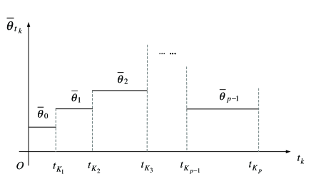
Figure 1: The dynamic signal of the desired orientations.

Denote the difference between the desired orientations at two contiguous time instants as $D_{k}=|\overline{\theta}_{k+1}-\overline{\theta}_{k}|$. We assume $\sum_{k=0}^{\infty}D_{k}<\infty$. Since what we concern is the tracking effect of the robots at each stage $[T_{k_{l-1}},T_{k_{l}}],l=1,2,\cdots$, we need to analyze the dynamical behavior of the leaders and followers stage by stage, and the ending states of the robots at the latest stage is just the starting states at the current stage. We give the main result for the system with dynamic leaders as follows.

Theorem 13.

Assume that the neighborhood radius satisfies $\sqrt{\frac{\log n}{n}}\ll r_{n}\ll 1$. Then for any given tracking error $\varepsilon>0$, we have for $i\in V$, $\lim_{t\rightarrow\infty}\left|v_{i}(t)-v_{n}\right|=0$ and

$$\max_{i\in V}\left|\theta_{i}(t_{K_{l+1}})-\overline{\theta}_{{l}}\right|\leq\varepsilon,\ \ l=0,1,2,\cdots,$$ (63)

if the ratio of the number of leaders satisfies one of the following conditions

1) $\vartheta\alpha_{n}\geq\frac{4v_{n}\tau_{n}(1+\sum_{k=0}^{\infty}D_{k}+|\overline{\theta}_{0}|)(1+o(1))}{\eta r_{n}}$ provided that $v_{n}\tau_{n}\gg\frac{\log n}{nr_{n}}$.

2) $\alpha_{n}\gg\frac{\log n}{nr_{n}^{2}}$ provided that $v_{n}\tau_{n}\ll\frac{\log n}{nr_{n}}$ or $v_{n}\tau_{n}=\Theta(\frac{\log n}{nr_{n}})$.

Proof. We first prove that for any pair of robots $i$ and $j$, we have

$$\left|\Delta_{ij}(t_{k})-\Delta_{ij}(0)\right|\leq\eta r_{n},\quad\forall k\geq 0.$$ (64)

Using Theorem 12, we see that (64) holds for $t\in[0,t_{K_{1}}]$ by taking $K_{1}\geq\Big{\lceil}\frac{\log(\varepsilon/(|\overline{\theta}_{0}|+L_{n})}{\log\widehat{\alpha}_{n}}\Big{\rceil}+1$. For $0\leq l\leq K_{1}$, we have $\max_{i\in V}|\alpha_{i}(t_{l})-\alpha_{i}(0)|\leq\frac{\alpha_{n}}{2}(1+o(1))$. Thus, $\max_{i\in V_{1}}|\theta_{i}(t_{K_{1}})-\overline{\theta}_{0}|\leq\widehat{\alpha}_{n}^{K_{1}-1}(|\overline{\theta}_{0}|+L_{n})\leq\varepsilon$, and $\max_{i\in V_{2}}|\theta_{i}(t_{K_{1}})-\overline{\theta}_{0}|\leq(1-\vartheta)\widehat{\alpha}_{n}^{K_{1}-1}(|\overline{\theta}_{0}|+L_{n})\leq(1-\vartheta)\varepsilon$, where $\widehat{\alpha}_{n}=\left(1-\frac{\vartheta\alpha_{n}(1+o(1))}{2}\right)$.

We now analyze the dynamical behavior of all agents for $k\in[K_{p}+1,K_{p+1}]$ $(p=2,3,\cdots)$ with $K_{p}=\Big{\lceil}\frac{\log(\varepsilon/(\varepsilon+D_{p-1}))}{\log\widehat{\alpha}_{n}}\Big{\rceil}+\sum_{s=1}^{p-1}K_{s}+1.$ We have at the time instant $t_{K_{p}}$, $\max_{i\in V_{1}}|\theta_{i}(t_{K_{p}})-\overline{\theta}_{p-1}|\leq\varepsilon$, and $\max_{i\in V_{2}}|\theta_{i}(t_{K_{p}})-\overline{\theta}_{p-1}|\leq(1-\vartheta)\varepsilon.$ At the time instant $t_{K_{p}+1}$, the desired orientation of leaders changes to $\overline{\theta}_{p}$, and the orientations of the followers and leaders at time $t_{K_{p}+1}$ satisfy $\max_{i\in V_{1}}|\theta_{i}(t_{K_{p}+1})-\overline{\theta}_{p}|\leq(1-\alpha_{i}(t_{K_{p}}))\Big{\{}\max_{i\in V_{1}}|\theta_{i}(t_{K_{p}})-\overline{\theta}_{p-1}|+D_{p-1}\Big{\}}+\alpha_{i}(t_{K_{p}})\Big{\{}\max_{i\in V_{2}}|\theta_{i}(t_{K_{p}})-\overline{\theta}_{p-1}|+D_{p-1}\Big{\}}\leq\varepsilon+D_{p-1}$, and $\max_{i\in V_{2}}|\theta_{i}(t_{K_{p}+1})-\overline{\theta}_{p}|\leq(1-\vartheta)(\varepsilon+D_{p-1})$, where $D_{p-1}=|\overline{\theta}_{p}-\overline{\theta}_{p-1}|$. Assume that (64) holds for $k_{0}\in[K_{p}+1,K_{p+1}],p=2,3,\cdots$. Then we have $\max_{i\in V}|\alpha_{i}(t_{l})-\alpha_{i}(0)|\leq\frac{\alpha_{n}}{2}(1+o(1))$ for $l\leq k_{0}$ . Using Lemmas 10 and 11, we have for $k\in[K_{p}+1,k_{0}],p=2,\cdots,P-1$, $\max_{i\in V_{1}}|\theta_{i}(t_{k})-\overline{\theta}_{p}|\leq\widehat{\alpha}_{n}^{k-K_{p}-1}(\varepsilon+D_{p-1})$, and $\max_{i\in V_{2}}|\theta_{i}(t_{k})-\overline{\theta}_{p}|\leq(1-\vartheta)\widehat{\alpha}_{n}^{k-K_{p}-1}(\varepsilon+D_{p-1}).$ Thus, the distance between agents $i$ and $j$ satisfies

$$|\Delta_{ij}(t_{k_{0}+1})-\Delta_{ij}(0)|\leq\Big{(}\sum_{s=0}^{p-1}\sum_{l=K_{s}+1}^{K_{s+1}}+\sum_{l=K_{p}+1}^{k_{0}}\Big{)}$$ (65)

$$\Big{\{}\Big{|}\int_{t_{l}}^{t_{l+1}}\left[v_{i}(t)\cos\theta_{i}(t)-v_{j}(t)\cos\theta_{j}(t)\right]dt\Big{|}$$

$$+\Big{|}\int_{t_{l}}^{t_{l+1}}\left[v_{i}(t)\sin\theta_{i}(t)-v_{j}(t)\sin\theta_{j}(t)\right]dt\Big{|}\Big{\}}$$

$$\leq 2(1+\widehat{\alpha}_{n})v_{n}\tau_{n}(1+o(1))\Big{(}\sum_{l=0}^{K_{1}}\widehat{\alpha}_{n}^{l-1}(|\overline{\theta}_{0}|+L_{n})$$

$$+\sum_{s=1}^{p-1}\sum_{k=K_{s}+1}^{K_{s+1}}\widehat{\alpha}_{n}^{l-K_{s}-1}(\varepsilon+D_{s-1})$$

$$+\sum_{l=K_{p}+1}^{k_{0}}\widehat{\alpha}_{n}^{l-K_{p}-1}(\varepsilon+D_{p-1})\Big{)}$$

$$+\sum_{l=0}^{k_{0}}(1+\widehat{\alpha}_{n})v_{n}\tau_{n}\widehat{\alpha}_{n}^{l-1}(1+o(1))$$

$$\leq 8v_{n}\tau_{n}\frac{1}{\vartheta\alpha_{n}}(1+o(1))\left(|\overline{\theta}_{0}|+\sum_{s=0}^{p-1}D_{s}+1\right)\leq\eta r_{n}.$$

By the above analysis, we see that for $k\in[K_{p}+1,K_{p+1}],p=0,1,\cdots,$ the assertion (63) holds, and we have for $l\geq 0$, $\max_{i\in V}|\alpha_{i}(t_{l})-\alpha_{i}(0)|\leq\frac{\alpha_{n}}{2}(1+o(1)).$ Moreover, using Lemma 11, we obtain

$$\max_{i\in V_{1}}\widetilde{v}_{i}(t_{k})\leq(\widehat{\alpha}_{n})^{k-1}\frac{v_{n}(1+o(1))}{2}\rightarrow 0,\ \ \hbox{as}\ \ k\rightarrow\infty,$$

$$\max_{i\in V_{2}}\widetilde{v}_{i}(t_{k})\leq(1-\vartheta)(\widehat{\alpha}_{n})^{k-1}\frac{v_{n}(1+o(1))}{2}\rightarrow 0,\ \ \hbox{as}\ \ k\rightarrow\infty.$$

$\square$

Remark 14.

A direct consequence is that the ratio of the number of leaders to the number of followers depends on the times and the amplitude that the desired orientations change during evolution.

3.4 A simulation example

We illustrate the feasibility of guiding a group of ordinary robots to accomplish a complicated task by introducing dynamic leaders whose desired orientation may change with the requirement of the task. The system is composed of $20$ ordinary agents labeled $1,2,\cdots,20$, and we aim to guide these robots to move to the right along the bottom line, go across an oval-shaped obstacle and not to collide with it as shown in Fig. 3. The desired orientations can be taken as $\overline{\theta}_{0}=0$, $\overline{\theta}_{1}=\frac{\pi}{2}$, $\overline{\theta}_{2}=0$ $\overline{\theta}_{3}=-\frac{\pi}{2}$, $\overline{\theta}_{4}=0$. To complete such a task, we introduce 3 leaders into the system which are labeled $21,22$ and $23$. The initial states of all agents are taken to satisfy Assumption 3 with the maximum initial speed $v=0.3$, and the neighborhood radius $r=0.3$. The dwell time is taken as $\tau=0.01$. The initial orientations, velocities and positions of the leaders and followers are listed in Fig. 2. Fig. 3 shows the trajectories of all robots, and we see that the leaders can guide the followers to achieve the pre-defined task.

Figure 2: The initial states of all agents in the simulation example.

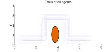
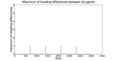
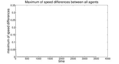
Figure 3: The trajectories of all robots, where the red and blue lines, respectively, denote the trajectories of the leaders and followers.

4 Concluding Remarks

In this paper, we proposed a sampled-data distributed control law for a group of nonholonomic unicycle robots, and established sufficient conditions for synchronization for the leaderless case without relying on dynamical properties of the neighbor graphs. In order to steer the system to a desired state, we then introduced leaders with constant or time-varying signals into the system, and provided the proportion of the leaders needed to track the static or dynamic signals. In our model, the robots are connected via distance-induced graphs, and a dwell time is assumed for the feasibility of information sensing and processing which as a consequence avoids issues such as chattering caused by abrupt changes of the neighbor relations. Some interesting problems deserve to be further investigated, for example, how to design the control law based on the information of relative orientations and relative positions, how to design the sampled-data control law to avoid collisions, and how to design the observer-based control laws for the case where the relative speed and relative orientation can not be directly measured.

Appendix Appendix A. Proof of the inequalities (2.2) and (30).

Proof of (2.2). By (14), we have $x_{i}(t_{k_{0}+1})-x_{i}(t_{k_{0}})=\int_{{t_{k_{0}}}}^{t_{{k_{0}}+1}}v_{i}(t)\cos\theta_{i}(t)dt$ and $y_{i}(t_{{k_{0}}+1})-y_{i}(t_{k_{0}})=\int_{t_{k_{0}}}^{t_{{k_{0}}+1}}v_{i}(t)$ $\sin\theta_{i}(t)dt$. Denote $X_{i}(t_{k})=(x_{i}(t_{k}),y_{i}(t_{k}))^{\prime}$. The distance between any two agents $i$ and $j$ satisfies the following inequality:

$$|\Delta_{ij}(t_{k+1})-\Delta_{ij}(t_{k})|$$ (A.69)

$$= \big{|}\|X_{i}(t_{k+1})-X_{j}(t_{k+1})\|-\|X_{i}(t_{k})-X_{j}(t_{k})\|\big{|}$$

$$\leq \|X_{i}(t_{k+1})-X_{i}(t_{k})-(X_{j}(t_{k+1})-X_{j}(t_{k}))\|$$

$$= \left\|\left(\begin{array}[]{c}\int_{t_{k}}^{t_{k+1}}[v_{i}(t)\cos\theta_{i}(t)-v_{j}(t)\cos\theta_{j}(t)]dt\\ \int_{t_{k}}^{t_{k+1}}[v_{i}(t)\sin\theta_{i}(t)-v_{j}(t)\sin\theta_{j}(t)]dt\\ \end{array}\right)\right\|$$

$$\leq \int_{t_{k}}^{t_{k+1}}\Big{\{}\left|v_{i}(t)\cos\theta_{i}(t)-v_{j}(t)\cos\theta_{j}(t)\right|$$

$$+\left|v_{i}(t)\sin\theta_{i}(t)-v_{j}(t)\sin\theta_{j}(t)\right|\Big{\}}dt.$$

Using (51), the first term of (A.69) satisfies

$$\int_{t_{k}}^{t_{k+1}}\left|v_{i}(t)\cos\theta_{i}(t)-v_{j}(t)\cos\theta_{j}(t)\right|dt$$ (A.70)

$$\leq \int_{t_{k}}^{t_{k+1}}|(v_{i}(t)-v_{j}(t))\cos\theta_{i}(t)|$$

$$+|v_{j}(t)(\cos\theta_{i}(t)-\cos\theta_{j}(t))|dt\leq\int_{t_{k}}^{t_{k+1}}\delta v(t)dt$$

$$+2\max_{1\leq i\leq n}v_{i}(t_{k})\int_{t_{k}}^{t_{k+1}}|\sin\frac{\theta_{i}(t)-\theta_{j}(t)}{2}|dt$$

$$\leq \int_{t_{k}}^{t_{k+1}}\delta v(t)dt+\max_{1\leq i\leq n}v_{i}(t_{k})\int_{t_{k}}^{t_{k+1}}\delta\theta(t)dt,$$

and the second term of (A.69) satisifies

$$\int_{t_{k}}^{t_{k+1}}\left|v_{i}(t)\sin\theta_{i}(t)-v_{j}(t)\sin\theta_{j}(t)\right|dt\leq\int_{t_{k}}^{t_{k+1}}\delta v(t)dt$$ (A.71)

$$+2\max_{1\leq i\leq n}v_{i}(t_{k})\int_{t_{k}}^{t_{k+1}}|\sin\frac{\theta_{i}(t)-\theta_{j}(t)}{2}|dt$$

$$\leq \int_{t_{k}}^{t_{k+1}}\delta v(t)dt+\max_{1\leq i\leq n}v_{i}(t_{k})\int_{t_{k}}^{t_{k+1}}\delta\theta(t)dt.$$

Substituting (A.70) and (A.71) into (A.69) yields the inequality (2.2). $\square$

Proof of (30). We see that if at the initial time instant, the distance between $i$ and $j$ satisfies $\Delta_{ij}(t_{0})<(1-\eta_{n})r_{n}$, then by (27) we have $\Delta_{ij}(t_{k})<r_{n}$; Otherwise, if $\Delta_{ij}(t_{0})\geq(1+\eta_{n})r_{n}$, then by (27) we have $\Delta_{ij}(t_{k})\geq r_{n}$. Compared with the initial time instants, the change of the agent $i$’s neighbors at time instant $t_{k}$ is characterized by the following set,

$$\mathcal{R}_{i}=\left\{j:(1-\eta_{n})r_{n}\leq\Delta_{ij}(0)\leq(1+\eta_{n})r_{n}\right\}.$$ (A.72)

Denote the maximum number of agents in the set $\mathcal{R}_{j}$ defined by (A.72) as $R_{\max}$. By the fact $P(B_{n})=1$ with $B_{n}$ defined in (19), we have for large $n$, $R_{\max}\leq 4n\pi\eta_{n}r_{n}^{2}(1+o(1))$. Since the inequality (27) holds for $l\leq k_{0}$, the number of each agent’s neighbors changed at time $t_{l+1}$ in comparison with its initial neighbors is bounded by $R_{\max}$. Using Lemma 3 in [tang2], we have for large $n$

$$\|P(t_{l+1})-P(0))\|\leq\frac{R_{\max}}{d_{\min}(0)}\cdot\frac{d_{\max}(0)-d_{\min}(0)}{d_{\min}(0)-R_{\max}}$$

$$\leq \frac{4n\pi\eta_{n}r_{n}^{2}}{\frac{1}{4}n\pi r_{n}^{2}}\cdot\frac{n\pi r_{n}^{2}+\frac{1}{4}n\pi r_{n}^{2}}{\frac{1}{4}n\pi r_{n}^{2}-4n\pi\eta_{n}r_{n}^{2}}(1+o(1)=80\eta_{n}(1+o(1)).$$

$\square$

Appendix Appendix B. Estimation of some characteristics for the leader-follower model.

By the fact $P(B_{n}^{\prime})=1$ with $B_{n}^{\prime}$ defined in (3.2), we can directly obtain the following results.

Lemma 15.

Let the neighborhood radius $r_{n}$ and the ratio $\alpha_{n}$ satisfy the conditions: $\sqrt{\log n/n}\ll r_{n}\ll 1$ and $\alpha_{n}\gg\frac{\log n}{nr_{n}^{2}}$. Then the following results hold almost surely for large $n$

1) For any agent $i\in V$, we have

$$\alpha_{i}(0)=\frac{\alpha_{n}}{1+\alpha_{n}}(1+o(1))=\alpha_{n}(1+o(1)).$$

2) The cardinality of the sets $\mathcal{N}_{i1}(0)$ and $\mathcal{N}_{i2}(0)$ satisfy

$$\min_{i\in V}d_{i1}(0)=\frac{n\pi r_{n}^{2}}{4}(1+o(1)),$$

$$\max_{i\in V}d_{i1}(0)=n\pi r_{n}^{2}(1+o(1));$$

$$\min_{i\in V}d_{i2}(0)=\frac{n\pi r_{n}^{2}\alpha_{n}}{4}(1+o(1)),$$

$$\max_{i\in V}d_{i2}(0)=n\pi r_{n}^{2}\alpha_{n}(1+o(1)).$$

3) The number of agents in the sets $\mathcal{R}_{i1}$ and $\mathcal{R}_{i2}$ satisfies

$$\max_{i\in V}r_{i}=4\eta\pi nr_{n}^{2}(1+o(1)),$$

$$\max_{i\in V}r_{i}^{\prime}=4\eta\pi n\alpha_{n}r_{n}^{2}(1+o(1)).$$

Lemma 16.

Under the assumptions in Lemma 15, the following assertions hold almost surely for large $n$

$$\max_{i\in V_{1}}|\widetilde{\theta}_{i}(t_{1})|\leq|\theta_{0}|+L_{n},$$

$$\max_{i\in V_{2}}|\widetilde{\theta}_{i}(t_{1})|\leq(1-w)(|\theta_{0}|+L_{n}),$$

$$\max_{i\in V_{1}}|\widetilde{v}_{i}(t_{1})|=\frac{v_{n}}{2}(1+o(1)),$$

$$\max_{i\in V_{2}}|\widetilde{v}_{i}(t_{1})|=(1-w)\frac{v_{n}}{2}(1+o(1)),$$

where $L_{n}=\frac{4C_{1}(1+o(1))}{\pi}\sqrt{\frac{\log n}{nr_{n}^{2}}}$.

References

- [1] \harvarditem Corts, Martnez, & Bullo2006rend Corts J., Martnez S., & Bullo F. \harvardyearleft2006\harvardyearright. Robust rendezvous for mobile autonomous agents via proximity graphs in arbitrary dimensions. IEEE Trans. Autom. Control, 51(8), 1289-1298.
- [2] \harvarditemSmith, Broucke, & Francis2007FranicesSmith S. L., Broucke M. E., & Francis B. \harvardyearleft2007\harvardyearright. Local control strategies for groups of mobile autonomous agents. IEEE Trans. Autom. Control, 52(6), 1154-1159.
- [3] \harvarditemPease, Shostak, & Lamport1980agreePease M., Shostak R., & Lamport L. \harvardyearleft1980\harvardyearright. Reaching agreement in the presence of faults. J. ACM, 27, 228-234.
- [4] \harvarditemLobel, & Ozdagar2011oz Lobel H., & Ozdagar A. \harvardyearleft2011\harvardyearright. Distributed subgradient methods for convex optimization over random networks. IEEE Trans. Autom. Control, 56(6), 1291-1306.
- [5] \harvarditemCao, Yu, & Anderson2011 formation Cao M., Yu C., & Anderson B. D. O. \harvardyearleft2011\harvardyearright. Formation control using range-only measurements. Automatica, 47(4), 776-781.
- [6] \harvarditemJadbabaie, Lin, & Morse2003Jad Jadbabaie A., Lin J., & Morse A. S. \harvardyearleft2003\harvardyearright. Coordination of groups of mobile autonomous agents using nearest neighbor rules. IEEE Trans. Autom. Control, 48(9), 988-1001.
- [7] \harvarditemRen, & Beard2005ren Ren W., & Beard R. W. \harvardyearleft2005\harvardyearright. Consensus seeking in multiagent systems under dynamically changing interaction topologies. IEEE Trans. Autom. Control, 50(5), 655-661.
- [8] \harvarditemOlfati-Saber, & Murry2004murry Olfati-Saber R., & Murray R. \harvardyearleft2004\harvardyearright. Consensus problems in networks of agents with switching topology and time-delays, IEEE Trans. Autom. Control, 49 (9), 1520-1533. \harvarditemMoshtagh, Michael, Jadbabaie, & Daniilidis2009vision1 Moshtagh N., Michael N., Jadbabaie A., and Daniilidis K. \harvardyearleft2009\harvardyearright. Vision-based, distributed control laws for motion coordination of nonholonomic robots. IEEE Trans. Robotics, 25(4), 851-860.
- [9] \harvarditemMontijano, Thunberg, Hu, & Sagüès2013vision2 Montijano E., Thunberg J., Hu X. M., & Sagüès C. \harvardyearleft2013\harvardyearright. Epipolar visual servoing for multirobot distributed consensus. IEEE Trans. Robotics, 29(5), 1212-1225.
- [10] \harvarditemMoreau2005moreau Moreau L. \harvardyearleft2005\harvardyearright. Stability of multiagent systems with time-dependent communication links. IEEE Trans. Autom. Control, 50(2), 169-181.
- [11] \harvarditemYu, Ren, Zheng, Chen, & L2013yuwenwu Yu W., Ren W., Zheng W., Chen G., & L J. \harvardyearleft2013\harvardyearright. Distributed control gains design for consensus in multi-agent systems with second-order nonlinear dynamics. Automatica, 49(7), 2107-2115.
- [12] \harvarditemXiao, & Wang2008zhangyaXiao F., & Wang L. \harvardyearleft2008\harvardyearright. Consensus protocols for discrete-time multi-agent systems with time-varying delays. Automatica, 44(10), 2577-2582.
- [13] \harvarditemWang, & Liu2009wanglinWang L., & Liu Z. X. \harvardyearleft2009\harvardyearright. Robust consensus of multi-agent systems with noise. Science in China: Information Science, 52(5), 824-834.
- [14] \harvarditemLi, & Zhang2009litao Li T., & Zhang J. F. \harvardyearleft2009\harvardyearright. Mean square average consensus under measurement noises and fixed topologies: necessary and sufficient conditions. Automatica, 45(8), 1929-1936. \harvarditemShi, & Johansson2013shiguodongShi G. D., & Johansson K. H. \harvardyearleft2013\harvardyearright. Robust consensus for continuous-time multi-agent dynamics. SIAM Journal on Control and Optimization, 51(5), 3673-3691.
- [15] \harvarditemGupta, & Kumar1999kumarGupta P., & Kumar P. R. \harvardyearleft1999\harvardyearright. Critical power for asymptotic connectivity in wireless networks. in Stochastic Analysis, Control, Optimization and Applications, Birkhauser Boston, Boston, MA, 547-566.
- [16] \harvarditemJi, & Egerstedt2007leader1Ji M., & Egerstedt M. \harvardyearleft2007\harvardyearright. Distributed coordination control of multiagent systems while preserving connectedness. IEEE Trans. Robotics, 23(4), 693-703.
- [17] \harvarditemDimarogonas, & Kyriakopoulos2007diamosDimarogonas D. V. ,& Kyriakopoulos K. J. \harvardyearleft2007\harvardyearright. On the rendezvous problem for multiple nonholonomic agents. IEEE Trans. Autom. Control, 52(5), 916-922.
- [18] \harvarditemDimarogonas, Tsiotras, & Kyriakopoulos2009diamos1 Dimarogonasa D. V., Tsiotras P.,& Kyriakopoulos K. J. \harvardyearleft2009\harvardyearrightLeader-follower cooperative attitude control of multiple rigid bodies. Systems and Control Letters, 58, 429-435. \harvarditemAjorlou, & Aghdam2013connecprevAjorlou A.,& Aghdam A. G. \harvardyearleft2013\harvardyearrightConnectivity preservation in nonholonomic multi-agent aystems: a bounded distributed control strategy, IEEE Trans. Autom. Control, 58(9), 2366-2371.
- [19] \harvarditemLiu, Li, Xie, Fu, & Zhang2013sampling1 Liu S., Li T., Xie L., Fu M.,& Zhang J. F. \harvardyearleft2013\harvardyearrightContinuous-time and sampled-data based average consensus with logarithmic quantizers. Automatica, 49(11), 3329-3336. \harvarditemXiao, & chen2012sampling2Xiao F., & Chen T. \harvardyearleft2012\harvardyearrightSampled-data consensus for multiple double integrators with arbitrary sampling. IEEE Trans. Autom. Control, 57(12), 3230-3235.
- [20] \harvarditemTang, & Guo2007tang2Tang G. G., & Guo L. \harvardyearleft2007\harvardyearrightConvergence of a class of multi-agent systems in probabilistic framework. Journal of Systems Science and Complexity, 20(2), 173-197. \harvarditemLiu, & Guo2009Auto Liu Z. X., & Guo L. \harvardyearleft2009\harvardyearrightSynchronization of multi-agent systems without connectivity assumption. Automatica, 45(12), 2744-2753.
- [21] \harvarditemLiu, Wang, & Hu2014ifac Liu Z. X., Wang J. H., & Hu X. M. \harvardyearleft2014\harvardyearrightSynchronization of Unicycle Robots with Proximity Communication Networks. Proc. of the 19th IFAC World Congress, 9197-9202, Cape Town, South Africa.
- [22] \harvarditemTove, Dimarogonas, Egerstedt, & Hu2010tovenTove G., Dimarogonas D. V., Egerstedt M., & Hu X. M. \harvardyearleft2010\harvardyearrightSufficient conditions for connectivity maintenance and rendezvous in leader-follower networks. Automatica, 46(1), 133-139. \harvarditemCao, Ren, & Li2009renwei2Cao Y., Ren W., & Li Y. \harvardyearleft2009\harvardyearrightDistributed discrete-time coordinated tracking with a time-varying reference state and limited communication. Automatica, 45(5), 1299-1305. \harvarditemCouzin, Krause, Franks, & Levy2005natureCouzin I. D., Krause J., Franks N. R., & Levy S. \harvardyearleft2005\harvardyearrightEffective leadership and decision-making in animal groups on the move. Nature, 433, 513-516. \harvarditemCao, Ren, & Egerstedt2012leaders1Cao Y. C., Ren W., & Egerstedt M. \harvardyearleft2012\harvardyearrightDistributed containment control with multiple stationary or dynamic leaders in fixed and switching directed networks. Automatica, 48(8), 1586-1597.
- [23] \harvarditemDimarogonas, Tsiotras, & Kyriakopoulos2009leaders2 Dimarogonas D. V., Tsiotras P., & Kyriakopoulos K. J. \harvardyearleft2009\harvardyearrightLeader-follower cooperative attitude control of multiple rigid bodies. Systems & Control Letters, 58(6), 429-435.
- [24] \harvarditemPenrose2003geometricPenrose M. \harvardyearleft2003\harvardyearrightRandom geometric graphs. Oxford University Press.
- [25] \harvarditemLiu, Han, & Hu2011auto2011Liu Z. X., Han J., & Hu X. M. \harvardyearleft2011\harvardyearrightThe proportion of leaders needed for the expected consensus. Automatica, 47(12), 2697-2703.
- [26]