Secret key capacity of the thermal-loss channel:
Improving the lower bound

Abstract

We consider the secret key capacity of the thermal loss channel, which is modeled by a beam splitter mixing an input signal mode with an environmental thermal mode. This capacity is the maximum value of secret bits that two remote parties can generate by means of the most general adaptive protocols assisted by unlimited and two-way classical communication. To date, only upper and lower bounds are known. The present work improves the lower bound by resorting to Gaussian protocols based on suitable trusted-noise detectors.

1 Introduction and relations with previous works

In recent years, the field of quantum information and communication has witnessed a growing interest in the area of continuous variable (CV) quantum systems [1]. Particularly successful has been the development of Gaussian quantum information [2] and the area of Gaussian quantum key distribution (QKD) [3]. The latter focuses on the implementation of protocols exploiting Gaussian states and operations. Gaussian states are easy to study because they are just characterized by their first two statistical moments, i.e., mean value and covariance matrix (CM) [2]. Furthermore, they are the easiest states that can be generated in quantum optics labs.

The research in Gaussian QKD has led to the design, the theoretical analysis and the experimental implementation of secure protocols in one-way [4, 5, 6, 7, 8, 9, 10, 11, 12, 13, 14, 15, 16, 17, 18], two-way [19, 20, 21, 22] and, more recently, measurement-device-independent configurations [23, 24]. Today state-of-the-art implementations of Gaussian QKD have been proven to be secure over distances of about $80$ km [25]. More so than distance, high rates are the promise of Gaussian protocols, with potential performances which are orders of magnitude higher than their discrete-variable (DV) counterpart [26]. High rates are important not only for secure quantum networks but, more generally, for any realistic design of a quantum Internet [27, 28].

From a theoretical point of view, it is therefore of fundamental importance to determine the optimal secret key rate that is achievable by two remote parties, say Alice and Bob, at the two ends of a quantum channel, especially if this channel is Gaussian. This optimal rate (capacity) is achieved by optimizing over the most general QKD protocols, which are based on local operations (LOs) assisted by unlimited two-way classical communication (CC), briefly called adaptive LOCCs. The presence of feedback makes these protocols very hard to study but, recently, Ref. 29 has introduced a novel methodology which fully simplifies the analysis of such protocols for the most important quantum channels for both CV and DV systems.

In fact, Ref. 29 has brought two important advances: (i) it has extended the notion of relative entropy of entanglement (REE) from quantum states to quantum channels; (ii) it has devised a novel technique based on teleportation [30, 31, 32], called ‘teleportation stretching’, able to reduce an arbitrary adaptive protocol into a much simpler block form, as long as the protocol is implemented at the ends of a quantum channel which suitably commutes with teleportation. By combining these two ingredients, Ref. 29 has computed the tightest-known upper bounds for the two-way quantum capacity $Q_{2}$ and the secret key capacity $K$ of many quantum channels, including DV Pauli channels, DV erasure channels and CV bosonic Gaussian channels. In particular, by showing coincidence with suitable lower bounds, Ref. 29 has established the secret-key capacities of dephasing channels, erasure channels, quantum-limited amplifiers and lossy channels. (For the erasure channel see also the independent derivation of Ref. 33 based on the different tool of the squashed entanglement [34, 35, 36].)

In the specific case of a lossy channel with arbitrary transmissivity $\eta$, Ref 29 has derived

$$Q_{2}(\eta)=K(\eta)=-\textrm{log}_{2}(1-\eta).$$ (1)

For high loss (i.e., long distances), this provides about $1.44$ secret bits per use, which is the fundamental rate-loss scaling which restricts any secure quantum optical communications. This is also the benchmark that a quantum repeater must surpass in order to be a meaningful device. The generalization of this scaling to repeater-assisted quantum communications and multi-hop quantum networks has been recently provided by Ref. 37. (See also Ref. 38 for the specific study of single-hop quantum communication networks.)

An important bosonic Gaussian channel which has not been fully solved by Ref 29 is the thermal-loss channel, which can be modeled by a beam splitter with transmissivity $\eta$, mixing the input signal mode with an environmental mode described by a thermal state with variance $\omega=2\bar{n}_{th}+1$, with $\bar{n}_{th}$ being the mean number of thermal photons. W still do not know the two-way quantum capacity $Q_{2}(\eta,\omega)$ and the secret key capacity $K(\eta,\omega)$ of this channel. We only know an upper bound, provided by the REE+teleportation method of Ref. 29, and a lower bound, first computed by Ref. 39 by using the notion of reverse coherent information [40]. In particular, these bounds provide the following sandwich for the secret key capacity

$$-\log_{2}\left(1-\eta\right)-h(\omega)\leq K(\eta,\omega)\leq\Phi(\eta,\omega)~{},$$ (2)

where

$$h(x):=\frac{x+1}{2}\log_{2}\frac{x+1}{2}-\frac{x-1}{2}\log_{2}\frac{x-1}{2},$$ (3)

and

$$\Phi(\eta,\omega):=\left\{\begin{array}[]{rl}&-\log_{2}[(1-\eta)\eta^{\bar{n}_{th}}]-h(\omega)\quad\text{for}~{}\bar{n}_{th}<\frac{\eta}{1-\eta}\\ &\\ &0\qquad\text{otherwise}\end{array}\right.$$ (7)

In this paper, we improve the lower bound present in Eq. (2). Our improved bound applies to the secret key capacity only (and not to the two-way quantum capacity), because it is based on the optimization of a class of QKD protocols. In fact, we consider a type of noise-assisted Gaussian QKD protocol which is a coherent version of the one considered in Ref. 8 (because it involves a quantum memory) and a direct generalization of the one studied in Ref. 39 (because it considers more general noise at the detection stage). In this protocol, Alice distributes one mode of a two-mode squeezed vacuum (TMSV) state through the thermal-loss channel, while keeping the other mode in a quantum memory. This is repeated many times. At the output of the channel, Bob s measurement setup consists of a beam splitter with arbitrary transmissivity and subject to a trusted-noise thermal environment; this is followed by homodyne detection, randomly chosen in one of the two quadratures. At the end of the quantum communication, Bob communicates which quadrature he has measured in each round. As a consequence, Alice performs the same sequence of homodyne detections on her systems and tries to infer Bob outcomes (reverse reconciliation). We compute the rate of this protocol, and we consider its optimization over the free parameters at Bob’s side. This will provide our improved lower bound.

The paper is structured as follows. In Sec. 2, we review the definition of the secret key capacity of a quantum channel. In Sec. 3, we review the main techniques and results of Ref. 29, which have led to the lower and upper bounds for the secret key capacity of the thermal-loss channel. In Sec. 4, we show the result of this work, i.e., how to improve the lower bound by means of the noise- and memory-assisted Gaussian QKD protocol. Finally, Sec. 5 is for the conclusions.

2 Secret key capacity of a quantum channel

Assume that Alice and Bob are connected by a quantum channel $\mathcal{E}$ over which they perform an adaptive protocol (see Ref. 29 for full details). After $n$ transmissions through $\mathcal{E}$, the two parties share an output state $\rho_{\mathbf{ab}}^{n}:=\rho_{\mathbf{ab}}(\mathcal{E}^{\otimes n})$ which depends on the sequence $\mathcal{L}=\{\Lambda_{0},\Lambda_{1},\ldots,\Lambda_{n}\}$ of adaptive LOCCs performed. The protocol is characterized by the triplet $(n,\epsilon,R^{n})$ where $\epsilon$ and the rate of the protocol $R^{n}$ are such that $||\rho_{\mathbf{ab}}^{n}-\phi_{n}||\leq\epsilon$ where $\phi_{n}$ is a target state with a content of information equal to $nR^{n}$ bits. By optimizing over all the possible LOCC-sequences $\mathcal{L}$ and by taking the limit of infinite channel uses $n\rightarrow\infty$, one defines the generic two-way capacity of the channel as follows

$$\mathcal{C}(\mathcal{E}):=\sup_{\mathcal{L}}\lim_{n\rightarrow\infty}R^{n}~{}.$$ (8)

Here we are interested in the optimal performance that can be achieved by QKD protocols over the quantum channel $\mathcal{E}$. In this scenario the two parties aim at generating secret bits, so that the target state $\phi_{n}$ is a private state [41]. The generic two-way capacity of Eq. (8) automatically defines the secret key capacity $\mathcal{C}(\mathcal{E})=K(\mathcal{E})$ of the channel: This is the maximum achievable number of secret bits that can be transmitted per channel use. In general the computation of the two-way capacities defined in Eq. (8) is extremely demanding. This is mainly due to the fact that we have to optimize over a family of LOCCs which entails feedback, which are exploited to optimize the subsequent inputs to the channel.

3 Bounds for the secret key capacity

3.1 Lower bound

The best-known lower bounds for the secret key capacity $K(\mathcal{E})$ are given by the (reverse) coherent information $I_{(RC)C}(\mathcal{E})$ of the channel. Consider a maximally entangled state of systems $A$ and $B$, i.e. an EPR state $\Phi_{AB}$. The propagation of half of such a state through the channel $\mathcal{E}$ defines its Choi matrix [42] $\rho_{\mathcal{E}}:=(\mathcal{I}\otimes\mathcal{E})\Phi_{AB}$. This allows us to introduce the coherent information [43, 44] of the channel $I_{C}(\mathcal{E})$ and its reverse counterpart [40, 39] $I_{RC}(\mathcal{E})$ which are defined as

$$I_{C(RC)}(\mathcal{E}):=S[\text{Tr}_{A(B)}(\rho_{\mathcal{E}})]-S(\rho_{\mathcal{E}})~{},$$ (9)

where $S$ is the von Neumann entropy. As a consequence of the hashing inequality [45], one may write (see Ref. 29 for more details)

$$\max\{I_{C}(\mathcal{E}),I_{RC}(\mathcal{E})\}\leq K(\mathcal{E})~{}.$$ (10)

For the specific case of the thermal-loss channel, the best lower bound is that provided by the reverse coherent information. In a thermal-loss channel $\mathcal{E}(\eta,\omega)$, the input signals are combined with thermal noise $\omega=2\bar{n}_{th}+1$, i.e., the input quadratures are transformed according to

$$\hat{x}\rightarrow\sqrt{\eta}\hat{x}+\sqrt{1-\eta}\hat{x}_{E}~{},$$ (11)

where $0\leq\eta\leq 1$ is the transmissivity and $\hat{x}_{E}$ is the environment in a thermal state with $\bar{n}_{th}$ mean photon number. The Choi matrix of this bosonic channel is energy-unbounded, so that it should be intended as an asymptotic limit of a suitable sequence of finite-energy states. In particular, the CV EPR asymptotic state $\Phi$ is defined as the limit for $\mu\rightarrow\infty$ of two-mode squeezed vacuum (TMSV) states [2] $\Phi^{\mu}=|\Phi^{\mu}\rangle\langle\Phi^{\mu}|$. In other words, we have

$$\rho_{\mathcal{E}}:=\lim_{\mu\rightarrow\infty}\rho^{\mu}~{},~{}~{}~{}\rho^{\mu}=(\mathcal{I}\otimes\mathcal{E})\Phi^{\mu}~{}~{}.$$ (12)

As a consequence, the reverse coherent coherent information of Eq. (9) is computed as follows

$$I_{RC}(\mathcal{E})=\lim_{\mu\rightarrow\infty}I_{RC}(\mathcal{E},\rho^{\mu})=\lim_{\mu\rightarrow\infty}S[\text{Tr}_{B}(\rho^{\mu})]-S(\rho^{\mu})~{}.$$ (13)

A direct evaluation for the thermal-loss channel leads to the following expression [39, 29]

$$I_{RC}(\eta,\omega)=-\log_{2}\left(1-\eta\right)-h(\omega).$$ (14)

3.2 Upper bound

As previously mentioned, a general upper bound for the secret key capacity of a quantum channel can be designed by extending the notion of relative entropy of entanglement (REE) from quantum states to quantum channels. Recall that for any bipartite state $\rho$ the REE is defined as $E_{R}(\rho)=\min_{\sigma}S(\rho||\sigma)$, where the minimization is taken over the set of all the possible separable states and $S(\rho||\sigma):=\text{Tr}[\rho(\log_{2}\rho-\log_{2}\sigma)]$ is the relative entropy.
By exploiting the properties of the REE, Ref. 29 showed that, at any dimension, the generic two-way capacity of Eq. (8) is upper bounded as follows

$$\mathcal{C}(\mathcal{E})\leq E_{R}^{\star}(\mathcal{E}):=\sup_{\mathcal{L}}\limsup_{n\rightarrow\infty}\frac{E_{R}(\rho_{\mathbf{ab}}^{n})}{n},$$ (15)

where $E_{R}^{\star}(\mathcal{E})$ is called the adaptive REE of the channel. The latter is very hard to compute. However, for a wide class of quantum channels, called teleportation-covariant or ‘stretchable’ channels [29], the adaptive REE of the channel $\mathcal{E}$ is simply bounded by the REE of its Choi matrix, i.e., one may write [29]

$$E_{R}^{\star}(\mathcal{E})\leq E_{R}(\rho_{\mathcal{E}})~{},$$ (16)

so that the computation of the upper bound in Eq. (15) is reduced to the much simpler computation of the single-letter quantity $E_{R}(\rho_{\mathcal{E}})$. Because this quantifies the amount of entanglement (REE) distributed through the channel by an EPR state, it can be called the entanglement flux of the channel [29] and is denoted as follows

$$\Phi(\mathcal{E}):=E_{R}(\rho_{\mathcal{E}})~{}.$$ (17)

Let us provide more details behind the crucial simplification of Eq. (16) which relies on the technique of teleportation stretching devised in Ref. 29.

3.2.1 Teleportation simulation of a channel and teleportation stretching of an adaptive protocol

Teleportation stretching allows us to reduce an adaptive protocol with an arbitrary associated quantum task (quantum information transmission, entanglement distribution or QKD) into an equivalent non-adaptive protocol, performing exactly the same original task but whose output state is expressed in a convenient block form. This reduction process can be exploited at any dimension, finite or infinite, whenever the quantum channel suitably commutes with the set $\mathbb{U}_{d}$ of the teleportation unitaries in dimension $d$. At finite dimension, the elements of $\mathbb{U}_{d}$ are represented by generalized Pauli operators. For CV systems $(d\rightarrow\infty)$, the set $\mathbb{U}_{\infty}$ is composed of displacement operators [32].

By definition, a quantum channel $\mathcal{E}$ is called “teleportation-covariant” or simply “stretchable” if, for any teleportation unitary $U\in\mathbb{U}_{d}$, we can write [29]

$$\mathcal{E}(U\rho U^{\dagger})=V\mathcal{E}(\rho)V^{\dagger}$$ (18)

for some unitary $V$. The key property of stretchable channels is represented by the fact that the teleportation unitaries can be pushed out of the channel and mapped into generally-different unitaries that can still be corrected. As a consequence of this property, the transmission of a quantum state through the channel $\mathcal{E}$ can be simulated by teleporting the state using the Choi matrix of the channel $\rho_{\mathcal{E}}$. Ref. 29 developed this teleportation-simulation argument for both DV and CV channels. (Note that the teleportation simulation of the specific class of DV Pauli channels was previously discussed in Refs. 46, 47).

Teleportation-simulation is only the first step of teleportation stretching. The technique of teleportation stretching involves the following main steps [29]: (i) first the stretchable channel is replaced with teleportation over its Choi matrix; (ii) teleportation is considered as an additional LOCC, while the Choi matrix is anticipated back in time and stretched out of the adaptive LOCCs; (iii) all the adaptive LOCCs are collapsed into a single trace preserving LOCC. By applying this procedure iteratively for all the $n$ transmissions, the output state shared by Alice and Bob can be expressed as follows [29]

$$\rho_{\mathbf{ab}}^{n}=\bar{\Lambda}(\rho^{\otimes n}_{\mathcal{E}})$$ (19)

in terms of a single and very complicated trace preserving LOCC $\bar{\Lambda}$. (Note that this result must not be confused with the content of Section V of Ref. 46 which instead showed how to transform a quantum communication protocol into an entanglement distillation protocol).

Let us now combine the Choi decomposition of Eq. (19) with Eq. (15). Using the properties of the REE, one derives [29]

$$E_{R}(\rho_{\mathbf{ab}}^{n})\overset{(1)}{\leq}E_{R}(\rho^{\otimes n}_{\mathcal{E}})\overset{(2)}{\leq}nE_{R}(\rho_{\mathcal{E}}),$$ (20)

where $(1)$ the REE is monotonically decreasing under trace preserving LOCCs and $(2)$ it is subadditive over tensor products. Thus, the complicated trace preserving LOCC $\bar{\Lambda}$ disappears in the chain of Eq. (20). Then, by substituting Eq. (20) into Eq. (15), one can also simplify the the upper limit and the supremum in the definition of $E_{R}^{\star}(\mathcal{E})$, obtaining [29]

$$\mathcal{C}(\mathcal{E})\leq E_{R}^{\star}(\mathcal{E})\leq E_{R}(\rho_{\mathcal{E}}):=\Phi(\mathcal{E})~{},$$ (21)

Thus, the secret key capacity of a stretchable channel is upper bounded by its entanglement flux, which is a single-letter computable quantity. This final result is achieved by combining the upper bound given by the adaptive REE of the channel with the technique of teleportation stretching.

3.2.2 Entanglement flux of the thermal-loss channel

It is easy to verify that bosonic Gaussian channels are stretchable. For a Gaussian channel, we can formally define its entanglement flux $\Phi(\mathcal{E})=E_{R}(\rho_{\mathcal{E}})=\min_{\sigma\in\text{SEP}}S(\rho_{\mathcal{E}}||\sigma)$ as [29]

$$\Phi(\mathcal{E}) :=\min_{\{\sigma^{\mu}\}}\liminf_{\mu\rightarrow\infty}S(\rho^{\mu}||\sigma^{\mu}),$$ (22)

where $\rho^{\mu}$ is given in Eq. (12) and the minimization is over all sequences $\{\sigma^{\mu}\}$ of separable states that converge in trace norm. This formulation takes into account of the fact that the Choi matrix of a Gaussian channel is energy unbounded. Therefore, the secret key capacity of a Gaussian channel satisfies [29]

$$K(\mathcal{E})\leq E^{\star}_{R}(\mathcal{E})\leq\Phi(\mathcal{E})\leq\liminf_{\mu\rightarrow\infty}S(\rho^{\mu}||\widetilde{\sigma}^{\mu})$$ (23)

for some (good) sequence of separable Gaussian states $\{\widetilde{\sigma}^{\mu}\}$. This choice is indeed crucial for having a good upper bound. By exploiting a simple formula for the relative entropy between Gaussian states proven in Ref. 29, one may compute $S(\rho^{\mu}||\widetilde{\sigma}^{\mu})$. For the thermal-loss channel, one finds the upper bound

$$\mathcal{C}(\mathcal{E})\leq\Phi({\eta,\omega}),$$ (24)

where $\Phi({\eta,\omega})$ is given in Eq. (7).

4 New lower bound for the secret key capacity of the thermal-loss channel

In this paper, we show the following result.

Theorem 4.1.

Consider a thermal-loss channel with transmissivity $\eta$ and thermal noise $\omega$. Its secret key rate $K(\eta,\omega)$ is lower-bounded by

$$R_{M}(\eta,\omega)=\underset{\eta_{d},\gamma}{\max}~{}R\left(\eta,\omega,\eta_{d},\gamma\right),$$ (25)

where

$$R\left(\eta,\omega,\eta_{d},\gamma\right) :=\frac{1}{2}\log_{2}\frac{\eta_{d}\omega+(1-\eta_{d})(1-\eta)\gamma}{\left(1-\eta\right)\left[\eta_{d}(1-\eta)\omega+\left(1-\eta_{d}\right)\gamma\right]}+h\left(\sqrt{\frac{\omega\left[\eta_{d}+(1-\eta)\left(1-\eta_{d}\right)\omega\gamma\right]}{\eta_{d}\omega+(1-\eta)\left(1-\eta_{d}\right)\gamma}}\right)-h(\omega),$$ (26)

and the maximization is over detection transmissivity $\eta_{d}$ and thermal variance $\gamma\geq 1$.

Proof.  Consider the Gaussian protocol described in Fig. 1. Alice has a TMSV state $\Phi^{\mu}$ of modes $a$ and $A$. This is a zero mean Gaussian state with CM

$$\mathbf{V}_{aA}=\left(\begin{array}[]{cc}\mu\mathbf{I}&\sqrt{\mu^{2}-1}\mathbf{Z}\\ \sqrt{\mu^{2}-1}\mathbf{Z}&\mu\mathbf{I}\end{array}\right):=\mathbf{V}_{\mathrm{TMSV}}(\mu),$$ (27)

where $\mathbf{I=}$diag$(1,1)$ and $\mathbf{Z=}$diag$(1,-1)$. Mode $a$ is kept in a quantum memory (for later measurement). Mode $A$ is sent through the thermal-loss channel with transmissivity $0\leq\eta\leq 1$ and thermal noise $\omega=2\bar{n}_{th}+1$. At the output, Bob implements a noisy detection. He uses a beam splitter of transmissivity $\eta_{d}$ to mix the output mode $B$ with a mode $v$ in a thermal state with variance $\gamma$, i.e., with CM

$$\mathbf{V}_{v}=\gamma\mathbf{I}.$$ (28)

The output $+$ of the beam splitter is then homodyned in the $q$ or $p$ quadrature, randomly. After (large) $n$ rounds, Bob communicates which quadrature he has measured in each round, so that Alice can perform exactly the same sequence of homodyne detections on the $a$-modes she has kept. Her outcomes are finally used to infer Bob’s outcomes (reverse reconciliation).

In the middle, between the two parties, the thermal-loss channel can be dilated into a beam splitter with transmissivity $\eta$ mixing the input mode $A$ with an environmental mode $E$, which is described by a thermal state with variance $\omega$. This thermal state can then be purified into a TMSV state of modes $e$ and $E$, which is completely under Eve’s control. This is known as an entangling cloner [48]. The CM of Eve’s input state is $\mathbf{V}_{eE}=\mathbf{V}_{\mathrm{TMSV}}(\omega)$. The output modes $e$ and $E^{\prime}$ are stored in a quantum memory which is coherently measured by Eve at the end of the protocol (collective attack).

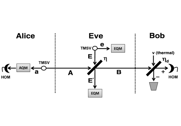
Figure 1: Noise-assisted Gaussian protocol. HOM = homodyne detection, TMSV = two-mode squeezed vacuum state, EQM = Eve’s quantum memory, AQM = Alice’s quantum memory. See text for explanations.

The initial global state of Alice, Bob and Eve is given by the tensor product $\rho_{0}=\rho_{aA}\otimes\rho_{eE}\otimes\rho_{v}$, with CM $\mathbf{V}_{0}=\mathbf{V}_{aA}\mathbf{\oplus V}_{eE}\mathbf{\oplus V}_{v}=\mathbf{V}_{aAeEv}$. For our convenience, we rearrange the modes so to obtain $\mathbf{V}_{0}=\mathbf{V}_{aeEAv}$. This state is processed by a sequence of two beam-splitters ($\eta$ and $\eta_{d}$). First we process mode $E$ and $A$, by applying the symplectic transformation $\mathbf{\tilde{V}}=\mathbf{S}_{\eta}\mathbf{V}_{0}\mathbf{S}_{\eta}^{T}$, where $\mathbf{S}_{\eta}:=\mathbf{I\oplus I\oplus T}(\eta)\oplus\mathbf{I}$, with

$$\mathbf{T}(\eta):=\left(\begin{array}[]{cc}\sqrt{\eta}\mathbf{I}&\sqrt{1-\eta}\mathbf{I}\\ -\sqrt{1-\eta}\mathbf{I}&\sqrt{\eta}\mathbf{I}\end{array}\right).$$ (29)

Then, we compute

$$\mathbf{V}=\mathbf{S}_{\eta_{d}}\mathbf{\tilde{V}S}_{\eta_{d}}^{T},~{}~{}\mathbf{S}_{\eta_{d}}:=\mathbf{I\oplus I\oplus I\oplus T}(\eta_{d})~{}.$$ (30)

The CM of Eq. (30) describes the global output state $\rho_{aeE^{\prime}+-}$. Discarding mode $-$ corresponds to considering the reduced state $\rho_{aeE^{\prime}+}=\mathrm{Tr}_{-}(\rho_{aeE^{\prime}+-})$ with CM $\mathbf{V}_{aeE^{\prime}+}$. From this CM we may compute Alice and Bob’s mutual information $I_{AB}$ as well as Eve’s Holevo information $\chi_{EB}$ on Bob’s outcomes (reverse reconciliation). Under ideal conditions of perfect reconciliation efficiency, the key rate is $R=I_{AB}-\chi_{EB}$.

To compute $I_{AB}$ we select from $\mathbf{V}_{aeE^{\prime}+}$, the block relative to mode $+$ measured by Bob. This is given by $\mathbf{V}_{+}=V_{B}\mathbf{I}$, where

$$V_{B}=\eta_{d}\left[\eta\mu+\left(1-\eta\right)\omega\right]+\left(1-\eta_{d}\right)\gamma:=V(\mu).$$ (31)

Note that Alice’s homodyne detection on mode $a$ of the TMSV state (after it is released by the memory) is equivalent to preparing Gaussianly-modulated squeezed states on mode $A$. Thus Bob’s conditional variance $V_{B|A}$ can be computed by simply setting $1/\mu$ in Eq. (31), i.e., we may write $V_{B|A}=V(1/\mu)$. Thus, we get

$$I_{AB}=\frac{1}{2}\log\frac{V_{B}}{V_{B|A}}\rightarrow\frac{1}{2}\log\frac{\eta_{d}\eta\mu}{\eta_{d}\left(1-\eta\right)\omega+\left(1-\eta_{d}\right)\gamma},~{}~{}\text{for large }\mu\text{. }$$ (32)

Eve’s Holevo function is $\chi_{EB}=S_{T}-S_{C}$, where $S_{T}$ is the von Neumann entropy of $\rho_{eE^{\prime}}$, while $S_{C}$ is that of the conditional state $\rho_{eE^{\prime}|B}$. From Eq. (30) consider the block

$$\mathbf{V}_{eE^{\prime}+}=\left(\begin{array}[]{cc}\mathbf{V}_{eE^{\prime}}&\mathbf{C}\\ \mathbf{C}^{T}&\mathbf{V}_{+}\end{array}\right),$$ (33)

where

$$\mathbf{V}_{eE^{\prime}}=\left(\begin{array}[]{cc}\omega\mathbf{I}&\sqrt{\eta\left(\omega^{2}-1\right)}\mathbf{Z}\\ \sqrt{\eta\left(\omega^{2}-1\right)}\mathbf{Z}&\left[\eta\omega+(1-\eta)\mu\right]\mathbf{I}\end{array}\right),~{}~{}~{}\mathbf{C=}\sqrt{\eta_{d}(1-\eta)}\left(\begin{array}[]{c}\sqrt{\omega^{2}-1}\mathbf{Z}\\ \sqrt{\eta}(\omega-\mu)\mathbf{I}\end{array}\right)~{}.$$ (34)

We compute the symplectic spectrum of $\mathbf{V}_{eE^{\prime}}$ which is given by $\left\{\nu_{1},\nu_{2}\right\}\overset{\mu}{\rightarrow}\left\{\omega,(1-\eta)\mu\right\}$. As a consequence, the von Neumann entropy $S_{T}=h(\nu_{1})+h(\nu_{2})$ takes the asymptotic form

$$S_{T}\overset{\mu}{\rightarrow}h(\omega)+\log_{2}\frac{e}{2}(1-\eta)\mu.$$ (35)

To compute the conditional term $S_{C}$, we note that, after the homodyne detection of quadrature $q$ ($p$), Eve’s CM is projected onto the conditional form

$$\mathbf{V}_{eE^{\prime}|B}=\mathbf{V}_{eE^{\prime}}-\mathbf{C}\left(\Pi\mathbf{V}_{+}\Pi\right)^{-1}\mathbf{C}^{T},$$ (36)

with $\Pi=$diag(1,0) ($\Pi=$diag(0,1)). From the CM of Eq. (36), after some algebra and taking the asymptotic limit, we obtain the following symplectic spectrum

$$\bar{\nu}_{1}\overset{\mu}{\rightarrow}\sqrt{\frac{\left(1-\eta\right)\left(\eta_{d}\omega+\left(1-\eta\right)\left(1-\eta_{d}\right)\gamma\right)}{\eta\eta_{d}}\mu,}$$ (37)

$$\bar{\nu}_{2}\overset{\mu}{\rightarrow}\sqrt{\frac{\omega\left[\eta_{d}+(1-\eta)\left(1-\eta_{d}\right)\omega\gamma\right]}{\eta_{d}\omega+(1-\eta)\left(1-\eta_{d}\right)\gamma}},$$ (38)

which provides the conditional entropy $S_{C}=h(\bar{\nu}_{1})+h(\bar{\nu}_{2})$. Combining this with Eq. (35), we derive the asymptotic Holevo bound

$$\chi_{EB}\overset{\mu}{\rightarrow}h(\omega)-h\left(\bar{\nu}_{2}\right)+\frac{1}{2}\log_{2}\frac{\left(1-\eta\right)\eta\eta_{d}\mu}{\eta_{d}\omega+\left(1-\eta_{d}\right)\left(1-\eta\right)\gamma}.$$ (39)

Finally, using Eqs. (32) and (39), we find formula of the asymptotic key rate, which is given in Eq. (26). $\blacksquare$

The secret key rate of Eq. (26) depends on Bob’s detection parameters, i.e., transmissivity $\eta_{d}$ and variance $\gamma$ (besides the parameters $\eta$ and $\omega$ of the channel). It can therefore be maximized over $\eta_{d}\in[0,1]$ and $\gamma\geq 1$, providing the optimized rate $R_{M}(\eta,\omega)$ of Eq. (25) which is our improved lower bound. It is easy to check that $R_{M}(\eta,\omega)$ outperforms all previously-known lower bounds. It is sufficient to show that the previous bounds can be retrieved for specific choices of the parameters $\eta_{d}$ and $\gamma$ in Eq. (26). By setting $\eta_{d}=1$ (no trusted noise at Bob’s side), it is easy to verify that we get $R(\eta,\omega,1,\gamma)=-\log_{2}\left(1-\eta\right)-h(\omega)$, corresponding to the lower bound of Eq. (2). According to the present derivation, a QKD protocol achieving $-\log_{2}\left(1-\eta\right)-h(\omega)$ corresponds to Alice distributing TMSV states through the channel, with Bob homodyning the output in $q$ or $p$; then, after many rounds, Bob informs Alice of his choices, so that she correspondingly homodynes the modes in her quantum memory to infer Bob’s outcomes. Then, by setting $\eta_{d}=1/2$ (balanced beam splitter) and $\gamma=1$ (vacuum noise), we also find

$$R(\eta,\omega,1/2,1)=\frac{1}{2}\log_{2}\frac{\omega+1-\eta}{\left(1-\eta\right)\left[(1-\eta)\omega+1\right]}+h\left(\sqrt{\frac{\omega\left[1+(1-\eta)\omega\right]}{\omega+(1-\eta)\gamma}}\right)-h(\omega),$$

which is Eq. (4) of Ref. 39. In Fig. 2, we numerically compare the maximized key rate $R_{M}(\eta,\omega)$ of Eq. (25) with respect to the other bounds, considering a thermal-loss channel with $\bar{n}_{th}=1$ thermal photon.

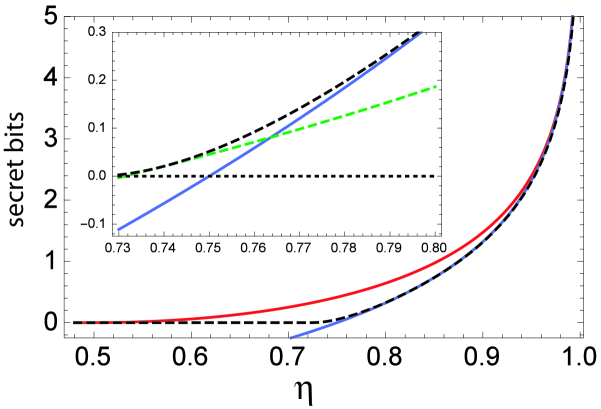
Figure 2: Secret bits versus transmissivity $\eta$ of a thermal-loss channel with $\bar{n}_{th}=1$ mean photon (i.e., $\omega=3$). The main plot compares the rate $R_{M}(\eta,\omega)$ of Eq. (25) (black-dashed) with the upper bound (red line) and lower bound (blue) of Eq. (2). In the inset we zoom a region of the main plot, where the optimal rate (black-dashed) is strictly greater than the lower bound (blue) of Eq. (2). We also show the performance of the protocol in the case where Bob employs a balanced beam splitter $\eta=1/2$ in a vacuum $\gamma=1$ (green dashed), which corresponds to Eq. (4) of Ref. 39.

5 Conclusions

In conclusion we have derived an improved lower bound for the secret key capacity of the thermal-loss channel, by optimizing the asymptotic key rate of a noise- and memory-assisted Gaussian QKD protocol in reverse reconciliation. There is a strict separation with respect to the previous best-known lower bounds derived in Ref. 39. Unfortunately, the improvement is small and the gap with the upper bound is still open. Further efforts must be devoted to close this gap and finally find the secret key capacity of this very important bosonic channel.

- [1] Braunstein, S. L. and van Loock, P., “Quantum information theory with continuous variables”, Rev. Mod. Phys. 77, 513 (2005).
- [2] Weedbrook C. et al., “Gaussian quantum information”, Rev. Mod. Phys. 84, 621 (2012).
- [3] Leverrier, A. and Diamanti, E., “Distributing Secret Keys with Quantum Continuous Variables: Principle, Security and Implementations”, Entropy 17(9), 6072-6092 (2015).
- [4] Grosshans, F., Van Assche, G., Wenger, J.,Tualle-Brouri, R. and Cerf, N.J., “High-rate quantum cryptography using Gaussian-modulated coherent states”, Nature 421, 238-241 (2003).
- [5] Weedbrook, C. et al., “Quantum Cryptography Without Switching”, Phys. Rev. Lett. 93, 170504 (2004).
- [6] Lance, A. M. et al., “No-Switching Quantum Key Distribution Using Broadband Modulated Coherent Light”, Phys. Rev. Lett. 95, 180503 (2005).
- [7] Silberhorn, Ch., Ralph, T.C., Lütkenhaus, N. and Leuchs G., “Continuous Variable Quantum Cryptography: Beating the 3 dB Loss Limit”, Phys. Rev. Lett. 89, 167901 (2002).
- [8] García-Patrón, R. and Cerf, N.,“Continuous-Variable Quantum Key Distribution Protocols Over Noisy Channels”, Phys. Rev. Lett. 102, 130501 (2009).
- [9] Filip, R., “Continuous-variable quantum key distribution with noisy coherent states”, Phys. Rev. A 77, 022310 (2008).
- [10] Usenko, V. C. and Filip, R., “Feasibility of continuous- variable quantum key distribution with noisy coherent states”, Phys. Rev. A 81, 022318 (2010).
- [11] Weedbrook, C., Pirandola, S. and Ralph, T. C., “Quantum Cryptography Approaching the Classical Limit”, Phys. Rev. Lett. 105, 110501 (2010).
- [12] Weedbrook, C., Pirandola, S., Lloyd, S. and Ralph, T. C., “Continuous-variable quantum key distribution using thermal states”, Phys. Rev. A 86, 022318 (2012).
- [13] Jacobsen, C. S, Gehring T., and Andersen, U. L., “Continuous Variable Quantum Key Distribution with a Noisy Laser”, Entropy, 17, 4654-4663 (2015).
- [14] Usenko, V. C. and Filip, R., “Trusted Noise in Continuous-Variable Quantum Key Distribution: A Threat and a Defense”, Entropy, 18(1), 20 (2016).
- [15] Usenko, V. C. and Grosshans, F., “Unidimensional continuous-variable quantum key distribution”, Phys. Rev. A, 92, 062337 (2015).
- [16] Leverrier, A., Grosshans, F. and Grangier, P., “Finite-size analysis of continuous-variable quantum key distribution”, Phys. Rev. A 81, 062343 (2010).
- [17] Leverrier, A., “Composable security proof for continuous-variable quantum key distribution with coherent states”, Phys. Rev. Lett. 114, 070501 (2015).
- [18] Furrer, F., et al., “Continuous Variable Quantum Key Distribution: Finite-Key Analysis of Composable Security against Coherent Attacks”, Phys. Rev. Lett. 109, 100502 (2012); see also Phys. Rev. Lett. 112, 019902(E) (2014).
- [19] Pirandola, S., Mancini, S., Lloyd, S. and Braunstein, S. L., “Continuous variable quantum cryptography using two-way quantum communication”, Nature Phys. 4, 726 (2008).
- [20] Ottaviani, C., Mancini, S. and Pirandola, S., “Two-way Gaussian quantum cryptography against coherent attacks in direct reconciliation”, Phys. Rev. A 92, 062323 (2015).
- [21] Ottaviani, C. and Pirandola, S., “General immunity and superadditivity of two-way Gaussian quantum cryptography”, Sci. Rep. 6, 22225 (2016).
- [22] Weedbrook, C., Ottaviani, C. and Pirandola, S., “Two-way quantum cryptography at different wavelengths”, Phys. Rev. A 89, 012309 (2014).
- [23] Pirandola, S. et al., “High-rate measurement-device-independent quantum cryptography”, Nature Photon. 9, 397-402 (2015).
- [24] Ottaviani, C., Spedalieri, G., Braunstein S. L. and Pirandola, S., “Continuous-variable quantum cryptography with an untrusted relay: Detailed security analysis of the symmetric configuration”, Phys. Rev. A 91, 022320 (2015).
- [25] Jouguet, P. et al., “Experimental demonstration of long-distance continuous-variable quantum key distribution” , Nature Photon. 7, 378-381 (2013).
- [26] Pirandola, S. et al., “MDI-QKD: Continuous- versus discrete-variables at metropolitan distances”, Nature Photon. 9, 773-775 (2015).
- [27] Kimble, H. J., “The Quantum Internet”, Nature 453, 1023-1030 (2008).
- [28] Pirandola, S. and Braunstein, S. L., “Unite to build a quantum internet”, Nature 532, 169 171 (2016).
- [29] Pirandola, S., Laurenza, R., Ottaviani, C. and Banchi, L., “Fundamental Limits of Repeaterless Quantum Communications”, Preprint arXiv.1510.08863 (2015).
- [30] Bennett, C. H., Brassard, G., Crepeau, C., Jozsa, R., Peres, A. and Wootters, W. K., “Teleporting an unknown quantum state via dual classical and Einstein-Podolsky- Rosen channels”. Phys. Rev. Lett. 70, 1895 (1993).
- [31] Braunstein, S. L. and Kimble, H. J., “Teleportation of continuous quantum variables”, Phys. Rev. Lett. 80, 869-872 (1998).
- [32] Pirandola, S. et al., “Advances in quantum teleportation”, Nature Photon. 9, 641-652 (2015).
- [33] Goodenough, K., Elkouss, D. and Wehner, S., “Assessing the performance of quantum repeaters for all phase-insensitive Gaussian bosonic channels”, Preprint arXiv:1511.08710 (2015).
- [34] Christandl, M., “The Structure of Bipartite Quantum States: Insights from Group Theory and Cryptography”, PhD thesis, University of Cambridge (2006).
- [35] Christandl, M. and Winter, A., “Squashed entanglement: An additive entanglement measure”, J. of Math. Phys. 45, 829-840 (2004).
- [36] Takeoka, M., Guha, S. and Wilde, M. M., “The Squashed Entanglement of a Quantum Channel”, IEEE Trans. Info. Theory 60, 4987-4998 (2014).
- [37] Pirandola, S., “Capacities of repeater-assisted quantum communications”, Preprint arXiv:1601.00966 (2016).
- [38] Laurenza, R. and Pirandola, S., “General bounds for sender-receiver capacities in multipoint quantum communications”, Preprint arXiv.1603.07262 (2016).
- [39] Pirandola, S., García-Patrón, R., Braunstein, S. L. and Lloyd, S., “Direct and Reverse Secret-Key Capacities of a Quantum Channel”, Phys. Rev. Lett. 102, 050503 (2009).
- [40] García-Patrón, Pirandola, S., Lloyd, S and Shapiro, J. H., “Reverse Coherent Information”, Phys. Rev. Lett. 102, 210501 (2009).
- [41] Horodecki, K., Horodecki, M., Horodecki, P. and Oppenheim, J., “Secure key from bound entanglement”, Phys. Rev. Lett. 94, 160502 (2005).
- [42] Choi, C., “Completely Positive Linear Maps on Complex matrices”, Linear Algebra Appl. 10, 285 290 (1975).
- [43] Lloyd, S., “Capacity of the noisy quantum channel”, Phys. Rev. A 55, 1613 (1997).
- [44] Schumacher, B. and Nielsen, M. A., “Quantum data processing and error correction”, Phys. Rev. A 54, 2629 (1996).
- [45] Devetak, I. and Winter, A., “Distillation of secret key and entanglement from quantum states”, Proc. R. Soc. A 461, 207 (2005).
- [46] Bennett, C. H., DiVincenzo, D. P., Smolin, J. A. and Wootters, W. K., “Mixed-state entanglement and quantum error correction”, Phys. Rev. A 54, 3824-3851 (1996).
- [47] Bowen, G. and Bose, S., “Teleportation as a Depolarizing Quantum Channel, Relative Entropy and Classical Capacity”, Phys. Rev. Lett. 87, 267901 (2001).
- [48] Grosshans, F., Cerf, N. J., Wenger, J., Tualle-Brouri, R., and Grangier P., “Virtual entanglement and reconciliation protocols for quantum cryptography with continuous variables”, Quantum Information & Computation 3 (7), 535-552 (2003).