Thermodynamics of anisotropic branes

Abstract

We study the thermodynamics of flavor D7-branes embedded in an anisotropic black brane solution of type IIB supergravity. The flavor branes undergo a phase transition between a ‘Minkowski embedding’, in which they lie outside of the horizon, and a ‘black hole embedding’, in which they fall into the horizon. This transition depends on the black hole temperature, its degree of anisotropy, and the mass of the flavor degrees of freedom. It happens either at a critical temperature or at a critical anisotropy. A general lesson we learn from this analysis is that the anisotropy, in this particular realization, induces similar effects as the temperature. In particular, increasing the anisotropy bends the branes more and more into the horizon. Moreover, we observe that the transition becomes smoother for higher anisotropies.

MPP-2016-275

1 Introduction

It is by now a well-established entry of the AdS/CFT dictionary duality that (a small number of) flavor degrees of freedom in the boundary gauge theory can be described, at strong coupling, in terms of (probe) flavor branes embedded in the dual geometry flavor . For the case of ${\cal N}=4$ super Yang-Mills (SYM) in four dimensions with gauge group $SU(N_{\textrm{\tiny c}})$ and $N_{\textrm{\tiny f}}$ flavors, this is done by considering $N_{\textrm{\tiny f}}$ D7-branes (with $N_{\textrm{\tiny f}}\ll N_{\textrm{\tiny c}}$, to avoid back-reaction) oriented along the $AdS_{5}$ directions and wrapping a $S^{3}\subset S^{5}$. At finite temperatures, the D7-branes have been shown to display an interesting thermodynamic behavior thermobrane , with a first order transition taking place between a phase in which they lie outside of the black hole horizon – the so-called ‘Minkowski embedding’ – and a phase in which they fall into it – the ‘black hole embedding’. In the gauge theory, this corresponds to a transition between a discrete, gapped meson spectrum and a continuous, gapless distribution of excitations.

Extending the holographic study of fundamental matter and its transitions to theories other than ${\cal N}=4$ SYM is clearly interesting in its own right. In fact, this has already been realized in various settings, see extensions for a few examples and reviewmesons for a review. A special motivation to look for more realistic theories comes from the realization that the quark-gluon plasma (QGP) formed in the collision of relativistic heavy ions rhic behaves as a strongly coupled fluid fluid . This has prompted in recent years the use of holography as a possible tool to describe such a system, in what has grown into a rather broad and active area of research. An overview of applications of holography to strongly coupled plasmas can be found, e.g., in reviewmateosetal .

In practice, the class of plasmas that can be described using holography is quite different from the QGP soup . One can nonetheless try to incorporate features of the real-world plasma in holographic models, to gain a qualitative understanding of its strong coupling behavior, which is of otherwise difficult access through ordinary field theoretical techniques. One such feature is the intrinsic anisotropy produced by having a privileged spatial direction in the problem, namely the direction of the beam of the scattering particles, called $z$-direction in the following. This anisotropy in the initial conditions of the collisions results into a so-called ‘elliptic flow’ of the plasma and in a peculiar phenomenology olli .

In the context of ${\cal N}=4$ SYM, this anisotropic state can be modeled at strong coupling in a top-down string construction by the introduction of a non-trivial axion field in the geometric background, as we shall review below MT ; MT2 . On the gauge theory side, one considers the action ALT

$$S=S_{{\cal N}=4}+\frac{1}{8\pi^{2}}\int\theta(z)\,\mathrm{Tr}F\wedge F\,,\qquad\theta(z)\propto z\,,$$ (1)

which is a marginally relevant deformation of the ${\cal N}=4$ SYM action, where the proportionality constant between the theta-angle $\theta(z)$ and $z$ has dimensions of energy and will be related to the parameter $a$ that we shall introduce in the next section. The rotational $SO(3)$ symmetry in the space directions is broken by the new term down to $SO(2)$ in the $xy$-plane.

Various observables have been computed for this plasma, see for example observables for a non-exhaustive list. However, one of the important phenomena that has so far eluded scrutiny are precisely the phase transitions of fundamental matter mentioned above. The theory in (1) has, in fact, only matter fields in the adjoint representation of the $SU(N_{\textrm{\tiny c}})$ gauge group. $N_{\textrm{\tiny f}}$ flavors of scalars and fermions in the fundamental representation may nonetheless be introduced and, with an abuse of language, we will refer to these fundamental fields indistinctly as ‘quarks’.

The main objective of this paper is to extend the study of thermobrane to the thermal, anisotropic state of MT ; MT2 , and to study how the anisotropy affects the physics of fundamental matter transitions. An important characteristic of the background is the presence of a conformal anomaly arising during renormalization, which introduces a length scale $\mu$ MT2 . As a consequence, the physics of the transitions will depend, separately, on the black hole temperature, its degree of anisotropy and the mass of the flavor degrees of freedom, all divided by $\mu$ in order to get dimensionless ratios. To simplify the analysis, we shall fix here the value of $\mu$ (in practice, by fixing the position of the black hole horizon) and consider instead two independent dimensionless ratios given by $a/M_{\textrm{\tiny q}}$ and $T/M_{\textrm{\tiny q}}$. We compute how the free energy depends on these two ratios for fixed $T/a$ and $a/T$, respectively. The punch line of our analysis will be that the anisotropy has very similar effects to those of the temperature: increasing the anisotropy bends the flavor branes more and more into the horizon facilitating the transition between Minkowski and black hole embeddings. We also discover a critical anisotropy at which, for fixed temperature and quark masses, the phase transition takes place. This is quite similar to what happens in the case of infinitely heavy quarkonia, whose anisotropy-induced melting was studied in melting .

This paper is organized as follows. In Sec. 2 we review the gravity set-up and in Sec. 3 we introduce probe D7-branes, considering both their black hole embedding and Minkowski embedding. In Sec. 4 we renormalize the brane on-shell action and compute the corresponding free energies. We conclude in Sec. 5 with a discussion of our results. Some of the more technical details of our computations are contained in a series of appendices.

2 Review of the gravity set-up

To model the gauge theory (1) at strong coupling and in a thermal state, we consider the type IIB supergravity geometry found in MT ; MT2 and given by

$$ds^{2}=\frac{L^{2}}{u^{2}}\left(-{\cal B}{\cal F}\,dt^{2}+dx^{2}+dy^{2}+e^{-\phi}dz^{2}+\frac{du^{2}}{{\cal F}}\right)+L^{2}\,e^{\frac{1}{2}\phi}d\Omega_{5}^{2}\,,$$ (2)

with $\Omega_{5}$ the volume form of a round 5-sphere. The dilaton $\phi$ and the metric fields ${\cal B}$ and ${\cal F}$ are solely functions of the radial coordinate $u$. This geometry contains a black brane, whose horizon is found at $u=u_{\textrm{\tiny H}}$, where ${\cal F}$ vanishes. The boundary of the space in these coordinates is at $u=0$. The gauge theory coordinates are $(t,x,y,z)$: we refer to the $z$-direction as the longitudinal (or anisotropic) direction and to $x$ and $y$ as the transverse directions. The radius $L$ is set to unity in the following, without loss of generality. The other supergravity fields that are turned on are the forms

$$F_{(5)}=4\left(\Omega_{5}+\star\Omega_{5}\right)\,,\qquad F_{(1)}=a\,dz$$ (3)

with $a$ being a parameter with dimensions of energy that controls the degree of anisotropy between the longitudinal $z$-direction and the orthogonal $xy$-plane. The potential for the 1-form is a linear axion, $\chi=a\,z$, with fixed radial profile, which is responsible for maintaining the system in an anisotropic equilibrium state.

The metric functions and the dilaton are known analytically in limiting regimes of low and high temperature MT2 , while for intermediate regimes one has to resort to numerics to solve Einstein field equations MT2 . For $u\to 0$ and any value of $a$, they asymptote to the $AdS_{5}\times S^{5}$ metric, ${\cal F}={\cal B}=1$ and $\phi=0$, while for $a=0$ they reduce to the black D3-brane solution

$${\cal B}=1\,,\qquad\phi=\chi=0\,,\qquad{\cal F}=1-\frac{u^{4}}{u_{\textrm{\tiny H}}^{4}}\,,$$ (4)

with temperature and entropy density given by

$$T_{\textrm{\tiny iso}}=\frac{1}{\pi u_{\textrm{\tiny H}}}\,,\qquad s_{\textrm{\tiny iso}}=\frac{\pi^{2}}{2}N_{\textrm{\tiny c}}^{2}T^{3}\,.$$ (5)

The anisotropic geometry has temperature and entropy density given instead by MT

$$T=\frac{e^{-\frac{1}{2}\phi_{\textrm{\tiny H}}}\sqrt{{\cal B}_{\textrm{\tiny H}}}(16+a^{2}u_{\textrm{\tiny H}}^{2}e^{\frac{7}{2}\phi_{\textrm{\tiny H}}})}{16\pi u_{\textrm{\tiny H}}}\,,\qquad s=\frac{N_{\textrm{\tiny c}}^{2}}{2\pi u_{\textrm{\tiny H}}^{3}}e^{-\frac{5}{4}\phi_{\textrm{\tiny H}}}\,,$$ (6)

where $\phi_{\textrm{\tiny H}}\equiv\phi(u=u_{\textrm{\tiny H}})$ and ${\cal B}_{\textrm{\tiny H}}\equiv{\cal B}(u=u_{\textrm{\tiny H}})$. This entropy density interpolates smoothly between the isotropic scaling (5) for small $a/T$ and the scaling MT ; ALT

$$s\simeq 3.21\,N_{\textrm{\tiny c}}^{2}T^{3}\left(\frac{a}{T}\right)^{\frac{1}{3}}\,,$$ (7)

for large $a/T$, so that the solution can be thought of as a domain-wall interpolating between AdS in the UV and a Lifshitz scaling in the IR. More details can be found in MT ; MT2 .

3 Flavor D7-brane embeddings

The scope of this paper is to study the thermodynamics of fundamental matter coupled to (1), which can be done at strong coupling by adding flavor D7-branes flavor to the geometry described above. The whole system can be thought of as a D3/D7/D7 construction with $N_{\textrm{\tiny D7}}$ anisotropy-inducing D7-branes and $N_{\textrm{\tiny f}}$ flavor D7-branes oriented as follows:

$$\begin{array}[]{l| cccc|c|ccc}&t&x&y&z&u&\vartheta&\varphi&\Omega_{3}\\ \hline\cr N_{\textrm{\tiny c}}~{}~{}\mbox{ D3 }&\times&\times&\times&\times&&&&\\ N_{\textrm{\tiny D7}}~{}\mbox{ D7 }&\times&\times&\times&&&\times&\times&\times\\ N_{\textrm{\tiny f}}~{}~{}~{}\mbox{ D7 }&\times&\times&\times&\times&\times&&&\times\end{array}\,,$$ (12)

where $(\vartheta,\varphi,\Omega_{3})$ are the coordinates on the $S^{5}$. The number of anisotropy inducing branes, $N_{\textrm{\tiny D7}}$, is arbitrary, and in fact can be as large as desired, resulting in a fully back-reacted geometry. On the other hand, the number of flavor branes, $N\textrm{\tiny f}$, must be small when compared to $N_{\textrm{\tiny c}}$, in order to avoid back-reaction and to consider them as probes. We emphasize that this construction is entirely top-down and the resulting geometry can be obtained from string theory.

As mentioned in the Introduction, the flavor D7-branes have two possible embeddings, one in which they lie outside of the horizon, called ‘Minkowski embedding’, and one in which they extend inside of the horizon, called ‘black hole embedding’. We now proceed to obtain the radial profile of these branes in both embeddings. To do so, it is convenient to start from the string frame metric (2) and to change the radial coordinate from $u$ to $\rho(u)$ with

$$\frac{d\rho}{du}=\frac{-\rho}{u\sqrt{{\cal F}(u)\,e^{\frac{1}{2}\phi(u)}}}\,.$$ (13)

We set $\rho(u_{\textrm{\tiny H}})=1$, resulting in

$$\rho=\exp{\int_{u_{\textrm{\tiny H}}}^{u}\frac{-du^{\prime}}{u^{\prime}\sqrt{{\cal F}(u^{\prime})\,e^{\frac{1}{2}\phi(u^{\prime})}}}}\,,$$ (14)

which can be inverted to obtain $u(\rho)$, needed in the following. In this new coordinate, the metric takes the form

$$ds^{2}=\frac{1}{{u(\rho)}^{2}}\left(-{\cal F}(\rho){\cal B}(\rho)dt^{2}+dx^{2}+dy^{2}+e^{-\phi(\rho)}dz^{2}\right)+\frac{e^{\frac{1}{2}\phi(\rho)}}{\rho^{2}}\left(d\rho^{2}+\rho^{2}d\Omega{{}^{2}_{5}}\right)\,.$$ (15)

The boundary is found at $\rho\rightarrow\infty$. The metric on the $S^{5}$ can be explicitly written as

$$d\Omega{{}^{2}_{5}}=d\vartheta^{2}+\cos^{2}\vartheta\,d\varphi^{2}+\sin^{2}\vartheta\,d\Omega{{}^{2}_{3}}\,.$$ (16)

As seen above, the D7-branes’ world-volume wraps the $(t,x,y,z,\Omega_{3})$ directions and it also extends along the radial direction $\rho$. To find their radial profile we need to compute the induced metric on the world-volume and solve the equations of motion for the embedding functions $\vartheta(\rho)$ and $\varphi(\rho)$. We analyze the black hole and Minkowski embeddings separately.

3.1 Black hole embedding

In the case of a black hole embedding, the radial profile is specified by $\psi(\rho)\equiv\cos\vartheta(\rho)$ and $\varphi=$ constant. The induced metric is given by

$${\left(d\rho^{2}+\rho^{2}d\Omega{{}^{2}_{5}}\right)}_{\textrm{\tiny ind}}=\left(1+\frac{\rho^{2}\psi^{\prime 2}}{1-\psi^{2}}\right)d\rho^{2}+\rho^{2}\left(1-\psi^{2}\right)d\Omega{{}^{2}_{3}}\,,$$ (17)

where the prime denotes a derivative with respect to $\rho$. Including the other world-volume directions, this results in

$$\sqrt{-g_{\textrm{\tiny ind}}}\propto\frac{e^{\frac{1}{2}\phi}}{\rho\,u^{4}}\sqrt{{\cal F}{\cal B}}\left(1-\psi^{2}\right)\sqrt{1-\psi^{2}+\rho^{2}\psi^{\prime 2}}\,,$$ (18)

where $u$ and the fields $\phi$, ${\cal F}$, and ${\cal B}$ have, again, to be considered functions of $\rho$. Notice that there is no Wess-Zumino term in the action, due to the particular orientation of the branes. To determine the profile $\psi(\rho)$ we solve its equation of motion. This follows from the action $S\propto\int e^{-\phi}\sqrt{-g_{\textrm{\tiny ind}}}$ and reads

$$\partial_{\rho}\left(P(\rho)\frac{\rho^{5}(1-\psi^{2})\psi^{\prime}}{\sqrt{1-\psi^{2}+\rho^{2}\psi^{\prime 2}}}\right)+P(\rho)\rho^{3}\frac{3\psi(1-\psi^{2})+2\rho^{2}\psi\psi^{\prime 2}}{\sqrt{1-\psi^{2}+\rho^{2}\psi^{\prime 2}}}=0\,,$$ (19)

where

$$P(\rho)=e^{-\frac{1}{2}\phi}{\left(\frac{1}{\rho\,u}\right)}^{4}\sqrt{{\cal F}{\cal B}}.$$ (20)

This equation is highly non-linear and has to be solved numerically, as we are going to do in a moment. The near-horizon expansion of $\psi$ needed to this scope is reported in App. A.

3.2 Minkowski embedding

In the case of a Minkowski embedding, the radial profile is conveniently specified by $\varphi=$ constant and a function $R(r)$, with $R=\rho\cos\vartheta$ and $r=\rho\sin\vartheta$. This results in the induced metric (the prime is now a derivative with respect to $r$)

$${\left(d\rho^{2}+\rho^{2}d\Omega{{}^{2}_{5}}\right)}_{\textrm{\tiny ind}}=\left(1+R^{\prime 2}\right)dr^{2}+r^{2}d\Omega{{}^{2}_{3}}$$ (21)

and the action

$$\sqrt{-g_{\textrm{\tiny ind}}}\propto\frac{e^{\frac{1}{2}\phi}}{u^{4}\rho^{4}}r^{3}\sqrt{{\cal F}{\cal B}}\sqrt{1+R^{\prime 2}}\,.$$ (22)

The equation of motion is found to be given by

$$\frac{dP(\rho)}{dR}r^{3}\sqrt{1+R^{\prime 2}}=\partial_{r}\left(P(\rho)\frac{r^{3}R^{\prime}}{\sqrt{1+R^{\prime 2}}}\right)\,,$$ (23)

where $P(\rho)$ is the same as above. Since this is a function of $\rho=\sqrt{r^{2}+R(r)^{2}}$, the derivatives with respect to $\rho$ and $r$ can be calculated in terms of $P^{\prime}(\rho)=dP/d\rho$. One obtains

$$P\left(\sqrt{r^{2}+R^{2}}\right)\partial_{r}\left(\frac{r^{3}R^{\prime}}{\sqrt{1+R^{\prime 2}}}\right)=P^{\prime}\left(\sqrt{r^{2}+R^{2}}\right)r^{3}\frac{(1+R^{\prime 2})R-rR^{\prime}}{\sqrt{1+R^{\prime 2}}\sqrt{r^{2}+R^{2}}}\,,$$ (24)

which, again, can be solved numerically, as we do next.

3.3 Numerical results

The inversion needed to express $u$ as a function of $\rho$ must be performed numerically for generic values of the anisotropy, due to the fact that the function ${\cal F}$ entering in (14) is generically not known analytically. Moreover, the equations to be solved are highly non-linear, which also requires a numerical approach. This can be readily done, resulting in the plots of Fig. 1, where the different profiles for the embeddings are represented. Analytic solutions are however possible in the limits of high and low temperature and are detailed in App. B.

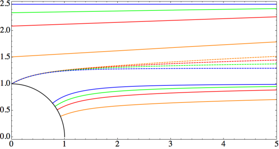
Figure 1: Profiles for various D7-brane embeddings in the $(R,r)$-plane. The black circle represents the horizon at $\rho=1$. Blue, green, red, and orange continuous lines (top to bottom in upper and lower group of curves) correspond respectively to $a/T=\{0,6.0,13.7,64.1\}$. The four continuous curves on the top correspond to the Minkowski embedding, whereas the four continuous curves on the bottom correspond to the black hole embedding. The four dotted curves in the middle correspond to the critical embedding, in which the branes touch the horizon at a single point.

Notice that the anisotropy has the effect of contributing to bending the brane towards the horizon: increasing the anisotropy of the background, the bending of the branes toward the horizon also increases. Moreover, anisotropic profiles converge to the flat geometry at larger distances. The critical embedding corresponds to a greater value of the asymptotic distance to the brane, holographically related to $M_{\textrm{\tiny q}}/T$. This means that the critical temperature $T_{\textrm{\tiny c}}$ is smaller in the anisotropic case. We can then already see that increasing the value of the anisotropy must have a similar effect as increasing the temperature of the black hole. We shall comment further upon this point after the computation of the free energy.

4 Thermodynamics of the flavor D7-branes

In order to study the thermodynamics of the flavor D7-branes, we need to evaluate their on-shell action for both embeddings. This will give the corresponding free energy. As usual, the on-shell action suffers from divergences due to the infinite volume of AdS, which need to be regularized using holographic renormalization reviewHR ; Karch:2005ms , as we do next.

4.1 Holographic renormalization

In what follows we shall work in Einstein frame, which is obtained by rescaling the metric (2) by a factor $e^{-\frac{1}{2}\phi}$:

$$ds^{2}=\frac{e^{-\frac{1}{2}\phi}}{u^{2}}\left(-\mathcal{FB}dt^{2}+dx^{2}+dy^{2}+e^{-\phi}dz^{2}+\frac{du^{2}}{\mathcal{F}}\right)+d\Omega_{5}^{2}\,.$$ (25)

This has the advantage of making the metric a direct product of an asymptotically AdS space with a round sphere. We also transform the radial coordinate $u$ to the Fefferman-Graham (FG) coordinate $v$ given by MT2

$$v=u-\frac{1}{12}a^{2}u^{3}+\left(-\frac{b_{4}+7f_{4}}{56}+\frac{1091}{32256}a^{4}-\frac{1}{16}a^{4}\log u\right)u^{5}+{\cal O}(u^{7})\,,$$ (26)

in terms of which the fields have the following near-boundary expansions

$$\phi = -\frac{1}{4}a^{2}v^{2}+\left(\frac{2}{7}b_{4}-\frac{47}{4032}a^{4}-\frac{1}{6}a^{4}\log{v}\right)v^{4}+\mathcal{O}(v^{6})\,,$$ (27)

$$\mathcal{F} = 1+\frac{11}{24}a^{2}v^{2}+\left(f_{4}+\frac{11}{144}a^{4}+\frac{7}{12}a^{4}\log{v}\right)v^{4}+\mathcal{O}(v^{6})\,,$$ (28)

$$\mathcal{B} = 1-\frac{11}{24}a^{2}v^{2}+\left(b_{4}-\frac{11}{144}a^{4}-\frac{7}{12}a^{4}\log{v}\right)v^{4}+\mathcal{O}(v^{6})\,,$$ (29)

and the metric (25) becomes

$$ds^{2}=\frac{dv^{2}}{v^{2}}+\frac{1}{v^{2}}g_{ij}dx^{i}dx^{j}+d\Omega_{5}^{2},$$ (30)

with

$$g_{tt} = -1+\frac{1}{24}a^{2}v^{2}+\left(\frac{2749}{16128}a^{4}-\frac{23}{28}b_{4}-\frac{3}{4}f_{4}+\frac{1}{24}a^{4}\log{v}\right)v^{4}+\mathcal{O}(v^{6}),$$ (31)

$$g_{xx} = g_{yy}=1-\frac{1}{24}a^{2}v^{2}+\left(\frac{71}{1792}a^{4}-\frac{5}{28}b_{4}-\frac{1}{4}f_{4}-\frac{1}{24}a^{4}\log{v}\right)v^{4}+\mathcal{O}(v^{6}),$$ (32)

$$g_{zz} = 1+\frac{5}{24}a^{2}v^{2}+\left(\frac{1163}{16128}a^{4}-\frac{13}{28}b_{4}-\frac{1}{4}f_{4}+\frac{1}{8}a^{4}\log{v}\right)v^{4}+\mathcal{O}(v^{6}).$$ (33)

In these expressions $f_{4}$ and $b_{4}$ are two coefficients that are not determined from the asymptotic equations of motion, as expected, but that can be extracted once a particular solution is known (either analytically in limiting regimes of small or large temperature or numerically for intermediate regimes MT2 ).

A further ingredient needed to continue the analysis is the boundary expansion of the embedding profile $\psi=\cos\vartheta$ introduced above. This can be obtained from the action

$$S_{\textrm{\tiny D7}}=-T_{\textrm{\tiny D7}}\textrm{vol}(S^{3})\int d^{4}x\,dv\,\frac{e^{\phi}}{v^{4}}\sqrt{-\text{det}(g_{ij})(1-\psi^{2})^{3}\left(\frac{1}{v^{2}}+\frac{\psi^{\prime 2}}{1-\psi^{2}}\right)}$$ (34)

and from the equation of motion resulting from it. In this formula, the prime denotes a derivative with respect to $v$. The asymptotic solution for $\psi$ turns out to be given by Jahnke:2013rca

$$\psi=mv+\left(c+\frac{5}{24}a^{2}m\log{v}\right)v^{3}+\mathcal{O}(v^{5}).$$ (35)

The parameters $m$ and $c$ are related to the quark masses and to the chiral condensate thermobrane . Using the expansions (33), integrating in $v$, and evaluating the action $S_{\textrm{\tiny D7}}$ at a cutoff $v=\epsilon\to 0$, one finds that it contains the following divergences:

$$\frac{S_{\text{div}}}{T_{\textrm{\tiny D7}}\textrm{vol}(S^{3})} = -\int d^{4}x\left(\frac{1}{4\epsilon^{4}}-\left(\frac{5}{48}a^{2}+\frac{1}{2}m^{2}\right)\frac{1}{\epsilon^{2}}+\frac{1}{12}a^{4}\log^{2}{\epsilon}\right.$$ (37)

$$\hskip 56.9055pt\left.+\left(\frac{47}{4032}a^{4}-\frac{5}{12}a^{2}m^{2}-\frac{2}{7}b_{4}\right)\log{\epsilon}+\mathcal{O}(\epsilon^{0})\right).$$

The task is now to cancel these divergences with appropriate counterterms and to extract the finite value of the action. In App. C, it is shown that (37) can be rewritten to get a more covariant appearance as

$$\frac{S_{\text{div}}}{T_{\textrm{\tiny D7}}\textrm{vol}(S^{3})} = -\int d^{4}xe^{\phi_{(0)}}\sqrt{-g_{(0)}}\left(\frac{a_{(0)}}{\epsilon^{4}}+\frac{a_{(1)}}{\epsilon^{2}}+(a_{(2)}-\phi_{(4)})\log{\epsilon}+a_{(3)}\log^{2}{\epsilon}+\mathcal{O}(\epsilon^{0})\right)\,,$$ (38)

with

$$a_{(0)}=\frac{1}{4},$$ (40)

$$a_{(1)}=-\frac{1}{4\epsilon^{2}}\left(\frac{5e^{2\phi}}{12}\partial^{i}\chi\partial_{i}\chi+2\psi^{2}\left(1-\frac{5e^{2\phi}}{12}\partial^{i}\chi\partial_{i}\chi\log{\epsilon}\right)\right),$$ (41)

$$a_{(2)}=-\frac{5e^{2\phi}}{12\epsilon^{4}}\psi^{2}\partial^{i}\chi\partial_{i}\chi\left(1-\frac{e^{2\phi}}{16}\partial^{i}\chi\partial_{i}\chi\log{\epsilon}\right),$$ (42)

$$a_{(3)}=\frac{e^{4\phi}}{12\epsilon^{4}}(\partial^{i}\chi\partial_{i}\chi)^{2},$$ (43)

and

$$e^{\phi_{(0)}}\sqrt{-g_{(0)}} = \epsilon^{4}\sqrt{-\gamma}e^{\phi}$$ (45)

$$\times\left(1+\frac{5e^{2\phi}}{24}\partial^{i}\chi\partial_{i}\chi+\frac{e^{4\phi}}{6}(\partial^{i}\chi\partial_{i}\chi)^{2}\left(\log{\epsilon}-\frac{1}{16}\right)-\frac{e^{6\phi}}{144}(\partial^{i}\chi\partial_{i}\chi)^{3}\log{\epsilon}\right)\,,$$

where $g_{(0)}=\det(g_{(0)ij})$ and $\gamma=\det(\gamma_{ij})$ is the determinant of the metric on the surface $v=\epsilon$.

Plugging (43)-(LABEL:phi_det) into (LABEL:divergences) and discarding finite terms suggests to consider the following counterterms

$$\begin{split}\frac{S^{(a)}_{\text{ct}}}{T_{\textrm{\tiny D7}}\textrm{vol}(S^{3})}=&\frac{1}{4}\int d^{4}x\sqrt{-\gamma}e^{\phi}\left(1-\frac{5e^{2\phi}}{24}\partial^{i}\chi\partial_{i}\chi-2\psi^{2}\right)\\ &+\frac{1}{24}\log{\epsilon}\int d^{4}x\sqrt{-\gamma}e^{3\phi}\left(e^{2\phi}(\partial^{i}\chi\partial_{i}\chi)^{2}-5\psi^{2}\partial^{i}\chi\partial_{i}\chi\right)\\ &+\frac{1}{12}\log^{2}{\epsilon}\int d^{4}x\sqrt{-\gamma}e^{5\phi}(\partial^{i}\chi\partial_{i}\chi)^{2}.\end{split}$$ (47)

We still need to take care of the term proportional to $\phi_{(4)}$. It is, of course, not possible to express $\phi_{(4)}$ solely in terms of $\phi$, so that one has to consider certain combinations of fields to remove the associated logarithmic divergence. Noticing that $\phi_{(4)}$ appears in

$$\int d^{4}x\sqrt{-\gamma}e^{\phi}=\int d^{4}x\left(\frac{1}{\epsilon^{4}}-\frac{5}{24\epsilon^{2}}a^{2}-\frac{1}{6}a^{4}\log{\epsilon}+\phi_{(4)}+\mathcal{O}(\epsilon^{2})\right),$$ (48)

one sees that a possible counterterm is given by

$$\frac{S_{\text{ct}}^{(b)}}{T_{\textrm{\tiny D7}}\textrm{vol}(S^{3})}=-\log{\epsilon}\int d^{4}x\sqrt{-\gamma}e^{\phi}\,.$$ (49)

This term introduces extra divergences, which can, however, be eliminated by a third counterterm

$$\frac{S^{(c)}_{\text{ct}}}{T_{\textrm{\tiny D7}}\textrm{vol}(S^{3})} = \log{\epsilon}\int d^{4}x\sqrt{-\gamma}\left(1-\frac{e^{2\phi}}{4}\partial^{i}\chi\partial_{i}\chi-\frac{7e^{5\phi}}{48}(\partial^{i}\chi\partial_{i}\chi)^{2}\right)$$ (51)

$$-\frac{1}{6}\log^{2}{\epsilon}\int d^{4}x\sqrt{-\gamma}e^{5\phi}(\partial^{i}\chi\partial_{i}\chi)^{2}.$$

The full counterterm action is then given by the sum of all the pieces above

$$S_{\text{ct}}=S_{\text{ct}}^{(a)}+S_{\text{ct}}^{(b)}+S_{\text{ct}}^{(c)}\,,$$ (52)

and reads

$$\frac{S_{\text{ct}}}{T_{\textrm{\tiny D7}}\textrm{vol}(S^{3})} = \frac{1}{4}\int d^{4}x\sqrt{-\gamma}e^{\phi}\left(1-\frac{5e^{2\phi}}{24}\partial^{i}\chi\partial_{i}\chi-2\psi^{2}\right)$$ (55)

$$+\log{\epsilon}\int d^{4}x\sqrt{-\gamma}\left(1-e^{\phi}-\frac{e^{2\phi}}{4}\partial^{i}\chi\partial_{i}\chi\left(1+\frac{5e^{\phi}}{6}\psi^{2}\right)-\frac{5e^{5\phi}}{48}(\partial^{i}\chi\partial_{i}\chi)^{2}\right)$$

$$-\frac{1}{12}\log^{2}{\epsilon}\int d^{4}x\sqrt{-\gamma}e^{5\phi}(\partial^{i}\chi\partial_{i}\chi)^{2}.$$

Notice that for $\phi=\chi=0$, this reduces, as it should, to

$$\frac{S_{\text{ct}}}{T_{\textrm{\tiny D7}}\textrm{vol}(S^{3})}=\frac{1}{4}\int d^{4}x\sqrt{-\gamma}(1-2\psi^{2})\,,$$ (56)

which is, up to finite terms, the expression found in thermobrane for the isotropic case.

With the addition of these counterterms to the divergent action, we obtain a regularized action $S_{\textrm{\tiny D7}}^{\text{reg}}=S_{\text{div}}+S_{\text{ct}}$, which is finite and reads

$$\begin{split}\frac{S_{\textrm{\tiny D7}}^{\text{reg}}}{T_{\textrm{\tiny D7}}\textrm{vol}(S^{3})}=&\int d^{4}x\left(\frac{1}{14}b_{4}-c\,m+\frac{5}{48}a^{2}m^{2}+\frac{241}{5376}a^{4}+\mathcal{O}(\epsilon)\right)\,.\end{split}$$ (57)

A few comments are in order at this point. First of all, we note that a priori there could be other scheme-dependent finite counterterms that would have to be included in (52), see Karch:2005ms . These counterterms are in fact vanishing in our case, since neither the metric nor the embedding profiles depend on the boundary coordinates. The axion does depend on $z$, but its field strength does not.

Second, there could in principle be a contribution from the conformal anomaly of the background MT2 , which enters at order ${\cal O}(a^{4})$, but this does not affect the phase transition between the Minkowski and black hole embeddings, since it only contributes to an additive overall shift to the free energy.

Finally, notice that the chiral condensate can be obtained from varying the renormalized action with respect to the quark mass and reads

$$\langle\bar{q}q\rangle=c-\frac{5}{24}a^{2}m\,.$$ (58)

This expression is exact in the anisotropy parameter $a$. The chiral condensate was also computed in thermobrane , where the authors showed that its value vanishes when $T/M_{q}$ approaches zero, as expected in an anomaly free gauge theory, like the one dual to the gravitational set up used in that work. The behavior of the condensate can be modified if the theory has an anomaly. To see that this can be the case, let us remember the Gell Mann-Oakes-Renner relation GellMann:1968rz , that in a construction like ours, where all the quark masses are equal to $M_{q}$, can be written as

$$f_{\pi}{m_{\pi}}^{2}=2M_{q}\langle\bar{q}q\rangle\,,$$ (59)

with $m_{\pi}$ being the mass of the pion and $f_{\pi}$ the pion decay rate, which is different from zero if the chiral currents are not conserved, that is, in the presence of an anomaly.

It is clear that the nature of the $m_{\pi}$ plays a relevant role here, and even if the meson spectrum has not been computed for our anisotropic background, in the context of the gauge/gravity correspondence with flavor Kruczenski:2003be , the mass of the pion, just like $M_{q}$, is expected to be proportional to the parameter $m$. From these considerations and the non vanishing $f_{\pi}$, given in our case by the anomaly in the gauge theory, the relation (59) suggests that $\langle\bar{q}q\rangle\sim m$, which is consistent with (58). We have numerically verified that for $a=0$ (resulting in $f_{\pi}=0$) we recover a vanishing $\langle\bar{q}q\rangle$ as $M_{q}/T$ goes to infinity. For non vanishing $a$, we have confirmed the monotonic growth of the condensate as the mass of the quark gets much larger than the temperature. This check was done numerically for values of $M_{q}/T$ with non vanishing $a$ which were not too large, since the integrand in (34) grows as we get farther from the horizon, compromising numerical stability. A detailed study of the behavior of the condensate in this limit would require a deeper understanding of the vacuum and the meson spectrum in this anisotropic theory, which is an interesting problem beyond the scope of this current investigation.

4.2 Free energy

At this point, we have all the ingredients to compute the free energy of the branes and determine which are the energetically favorable configurations. The free energy is notoriously given by the on-shell Euclidean action, which we now compute.

Switching back to the $u$ coordinate and expanding all the fields around the boundary to compute the counterterm action, one can show after some trivial albeit tedious manipulations that the regularized action becomes

$$\begin{split}\frac{S_{\textrm{\tiny D7}}^{\text{reg}}}{T_{\textrm{\tiny D7}}\textrm{vol}(S^{3})}=&\frac{1}{T}\left(G(m)-\frac{355}{32256}a^{4}+c\,m-\frac{a^{2}m^{2}}{48}-\frac{5}{56}b_{4}-\frac{1}{8}f_{4}-\frac{1}{4}m^{4}-\frac{1}{4u_{\textrm{\tiny H}}^{4}}\right.\\ &\left.+\frac{a^{2}+24m^{2}}{48u_{\textrm{\tiny H}}^{2}}-\log{u_{\textrm{\tiny H}}}\left(\frac{299a^{4}}{4032}-\frac{5a^{2}m^{2}}{12}-\frac{2b_{4}}{7}\right)-\frac{1}{12}a^{4}\log^{2}{u_{\textrm{\tiny H}}}\right),\end{split}$$ (60)

where the integral

$$\begin{split}G(m)=\int_{u_{\text{boundary}}}^{u_{\textrm{\tiny H}}}du&\left(\frac{e^{-\frac{3}{4}\phi}}{u^{5}}(1-\psi^{2})\sqrt{\mathcal{B}(1-\psi^{2}+e^{\frac{1}{2}\phi}u^{2}\mathcal{F}\psi^{\prime 2})}+\frac{a^{4}}{6u}\log{u}\right.\\ &\left.+\frac{1}{u^{3}}\left(\frac{a^{2}}{24}+m^{2}\right)+\frac{1}{u}\left(\frac{299a^{4}}{4032}-\frac{5a^{2}m^{2}}{12}-\frac{2b_{4}}{7}\right)-\frac{1}{u^{5}}\right)\end{split}$$ (61)

is finite by construction. The free energy is related to this action by

$$F=T\,S_{\textrm{\tiny D7}}^{\text{reg}}.$$ (62)

Notice that in the expressions (60)-(61) above there appear various geometrical parameters that originate from the expansions of the fields and are unphysical quantities. We would like instead to find a final result only in terms of the physical observables $a$, $T$, and the quark mass $M_{\textrm{\tiny q}}$. To this scope, we need to find the explicit map between the two sets of parameters

$$(u_{\textrm{\tiny H}},\phi_{\textrm{\tiny H}},{\cal B}_{\textrm{\tiny H}},m,\ldots)\quad\to\quad(a,T,M_{\textrm{\tiny q}})\,.$$ (63)

First of all, we notice that since the flavor branes are probes in a fixed geometry, the relation between $T$ and $(u_{\textrm{\tiny H}},\phi_{\textrm{\tiny H}},{\cal B}_{\textrm{\tiny H}})$ has to be the same as in the case without the branes MT2 , namely (6). The same is true for $a$, which is also fixed once we fix the background MT2 . What is then left to do is to extract the dependence of $M_{\textrm{\tiny q}}$ on these parameters.

Finally, we can plot (60) as a function of the various parameters. Out of the dimensionful parameters $a$, $T$, and $M_{\textrm{\tiny q}}$ we can form two dimensionless ratios, which we pick to be $a/M_{\textrm{\tiny q}}$ and $T/M_{\textrm{\tiny q}}$. The former choice has the advantage of displaying the similarity between anisotropy and temperature, while the latter choice allows for a more immediate comparison with the isotropic results present in the literature. Note that the background itself is not invariant under simultaneous rescaling of $a$ and $T$ even if the ratio $a/T$ is kept fixed MT2 . Consequently we do not expect our results to be invariant under a similar rescaling, even if the adimensional variables are kept fixed. Nonetheless, we explore a range of values for the parameters $T$, $a$ and $M_{\textrm{\tiny q}}$ and even if the particulars change, the general behavior is the same, and the same conclusions can be reached.

In Fig. 2, we plot the free energy as a function of $a/M_{\textrm{\tiny q}}$ for different values of $T/a$. The free energy is divided by $T\,K$, where $K=T_{\textrm{\tiny D7}}\mbox{vol}(S^{3})\mbox{vol}(x)N_{\textrm{\tiny f}}$ scales like $T^{3}$, making the quantity on the vertical axis adimensional. In order to better understand the order of the phase transition, we zoom in Fig. 3 over the parameter region in which the transition takes place. At small anisotropy and large temperature, the plots display the “swallow tail” structure (Fig. 3 (a) and (b)), which is typical of first order phase transitions, with a discontinuous first order derivative of the curve. This is in agreement with the findings of thermobrane . Increasing the anisotropy over temperature, however, the swallow tail disappears, smoothing out the curve (Fig. 3 (c) and (d)). We discover then an interesting consequence of the introduction of this extra parameter in the system: the order of the transition between the Minkowski and black hole phases depends on the value of the anisotropy and grows with it.

Figure 2: Free energy as a function of $a/M_{\textrm{\tiny q}}$ for fixed values of $T/a$. From left to right, we have fixed $T/a=$25.3 (red), 4.38 (blue), 1.81 (green), and 0.72 (orange). The dashed part of the lines represents the Minkowski embedding, whereas the continuous part represents the black hole embedding. Here $K=T_{\textrm{\tiny D7}}\mbox{vol}(S^{3})\mbox{vol}(x)N_{\textrm{\tiny f}}$.

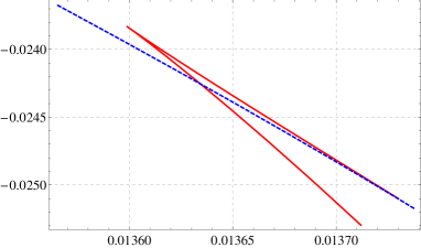
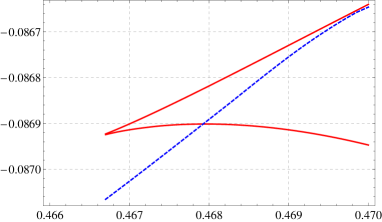
(a)	(b)
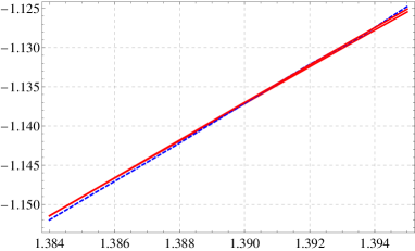
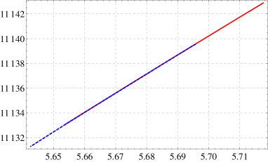
(c)	(d)

Figure 3: Zoom into the transition region between the Minkowski and black hole embeddings. The values of the temperature are $T/a=$ 25.3 (a), 0.72 (b), 0.22 (c), and 0.04 (d). The blue, dashed line represents the Minkowski embedding, whereas the solid, red line represents the black hole embedding. Here $K=T_{\textrm{\tiny D7}}\mbox{vol}(S^{3})\mbox{vol}(x)N_{\textrm{\tiny f}}$.

From Fig. 2, it is also obvious that the critical value of $a/M_{\textrm{\tiny q}}$ at which the transition takes place increases as we decrease $T/a$. This critical anisotropy as a function of the temperature is detailed in Fig. 4.

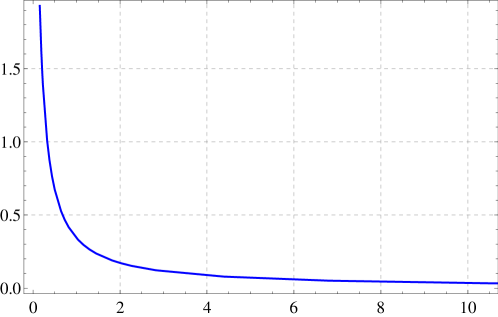
Figure 4: Critical anisotropy as a function of the temperature.

In Fig. 5, we plot the free energy as a function of $T/M\textrm{\tiny q}$ for fixed values of $a/T$. In Fig. 6 we zoom over the region of the phase transition and we see again a very similar behavior as the one in Fig. 3: increasing the anisotropy has the effect of smoothing out the transition which, starting from first order for small $a/T$ (Fig. 6 (a) and (b)), becomes of higher order (Fig. 6 (c) and (d)).

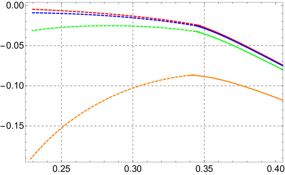
Figure 5: Free energy as a function of $T/M\textrm{\tiny q}$ for fixed values of $a/T$. From top to bottom, we have fixed $a/T=$0.03 (red), 0.22 (blue), 0.55 (green), and 1.37 (orange). The dashed part of the lines represents the Minkowski embedding, whereas the continuous part represents the black hole embedding. Here $K=T_{\textrm{\tiny D7}}\mbox{vol}(S^{3})\mbox{vol}(x)N_{\textrm{\tiny f}}$. Notice how increasing the value of the anisotropy from (a) to (d), the discontinuity in the derivative of the curves smooth out, signalling an increase of the order of the phase transition.

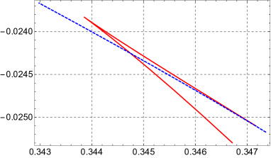
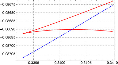
(a)	(b)
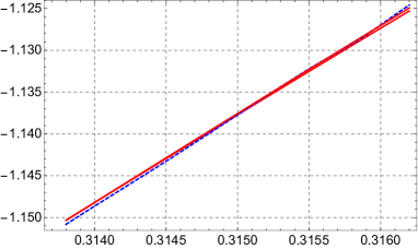
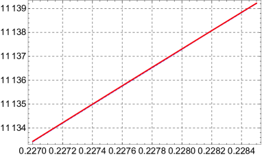
(c)	(d)

Figure 6: Zoom into the transition region between the Minkowski and black hole embeddings. The values of the anisotropy are $a/T=$ 0.03 (a), 1.37 (b), 4.41 (c), and 24.9 (d). The blue, dashed line represents the Minkowski embedding, whereas the solid, red line represents the black hole embedding. Here $K=T_{\textrm{\tiny D7}}\mbox{vol}(S^{3})\mbox{vol}(x)N_{\textrm{\tiny f}}$. As in Fig. 3, we see that increasing the anisotropy from (a) to (d) smooths out the transition region of the curves.

The critical temperature as a function of the anisotropy is reported in Fig. 7. Comparing with Fig. 4 we see that the decrease of the critical temperature with the increase of the anisotropy is much slower than the decrease of the critical anisotropy with the increase of the temperature in that plot.

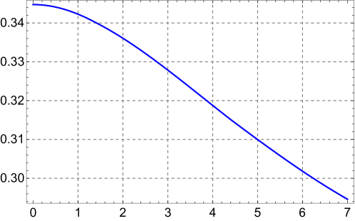
Figure 7: Critical temperature as a function of the anisotropy.

4.3 Entropy

Another interesting thermodynamical quantity is the entropy density, which is given by taking the derivative of the free energy with respect to the temperature

$$S=-\frac{\partial F}{\partial T}\,,$$ (64)

while maintaining $a/M_{\textrm{\tiny q}}$ fixed. In order to take this derivative, we need to recompute the free energy while maintaining this new ratio fixed. The results for the free energy and the entropy density are plotted in Figs. 8-9.

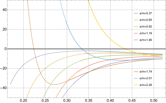
Figure 8: Free energy as a function of the temperature for $a/M_{\textrm{\tiny q}}$ fixed. The decreasing curves (in yellow, blue and brown) have, from left to right, $a/M_{\textrm{\tiny q}}=1.74,2.01,2.28$. The increasing curves have, from left to right, $a/M_{\textrm{\tiny q}}=0.37,0.65,0.92,1.19,1.46$. As usual, the dashed regions of the curves correspond to the Minkowski embedding, whereas the solid regions correspond to the black hole embeddings.

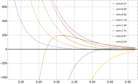
Figure 9: Entropy density as a function of the temperature for $a/M_{\textrm{\tiny q}}$ fixed. The increasing curves (in yellow, blue and brown) have, from left to right, $a/M_{\textrm{\tiny q}}=1.74,2.01,2.28$. The decreasing curves have, from left to right, $a/M_{\textrm{\tiny q}}=0.37,0.65,0.92,1.19,1.46$. As usual, the dashed regions of the curves correspond to the Minkowski embedding, whereas the solid regions correspond to the black hole embeddings.

5 Discussion

In this paper we have studied fundamental matter phase transitions in a strongly coupled plasma with a spatial anisotropy, using holography. This has been done by considering the embedding of flavor D7-branes in a type IIB supergravity solution with a non-vanishing, anisotropy-inducing axion field. In a heavy ion collision experiment, the anisotropic direction would correspond to the beam direction. The flavor branes allow for the introduction of degrees of freedom in the fundamental representation of the gauge group, which we have called quarks with a slight abuse of language. We have considered the so-called quenched flavor approximation, in which the number of quark flavors $N_{\textrm{\tiny f}}$ is much smaller than the number of colors $N_{\textrm{\tiny c}}$, in order to have probe branes in a fixed background geometry. It is important to notice that these quarks are allowed to have finite mass (which is controlled by the radial position of the D7-branes) and are therefore dynamical particles. In this regard, this work extends the analysis done in melting , where the physics of infinitely heavy mesons was investigated.

We have focused on the transition which happens between a phase in which the D7-branes lie outside of the black hole horizon present in the background and a phase in which they fall into the horizon. The corresponding physics in the dual gauge theory side is that of a transition between a discrete meson spectrum with a mass gap and a continuous, gapless spectrum thermobrane . It is important to stress that the transition studied here is not a confinement/deconfinement transition (as the background geometry always contains a black hole horizon), but a transition of fundamental matter, which can survive in a bound state even if the surrounding plasma is deconfined.

Interestingly, the order of the transition depends on the degree of anisotropy of the system, with higher anisotropies making the transition smoother. It would be interesting to determine precisely the order of the phase transition and the critical exponents as functions of the parameter $a$. Complex critical exponents signal a first-order transition, while real exponents a higher order transition. To compute these quantities, a near-horizon scaling analysis along the lines of the one performed in thermobrane ; yaffe woule be required.

From a technical point of view, a novelty of this paper is represented by the renormalization procedure that we have adopted in order to compute the free energy. There appear divergent terms that go like a logarithm squared of the cutoff, which have been eliminated with an appropriate set of counterterms. We have also obtained an analytic exact expression for the chiral condensate as a function of the anisotropy parameter. However, the main general lesson we can draw from our computations is that, besides a critical temperature, there is also a critical anisotropy at which the transition can happen, at fixed temperature. In fact, the anisotropy seems to play a very similar role as the temperature: increasing the anisotropy bends the D7-branes more and more toward the black hole horizon. This confirms the findings of melting , where the anisotropy was seen as being a possible mechanism for the dissociation of heavy quarkonium.

This can be heuristically understood as the brane being ‘pulled’ more strongly into the horizon due to the anisotropy. This has to do with the gravitational strength at the particular position in which the brane is located. In the isotropic case, there is only one way in which the gravitational pull changes along the bulk, so increasing the gravitational pull at a certain position implies increasing it in all the bulk. The non-trivial axion gives cause for new behavior, because it has the effect of making the gravitational pull change more drastically, in such a way that the branes get to feel the same gravitational pull ‘earlier’, that is, while being located further from the horizon. The reason why $a/m$ acts similarly to $T/m$ is that in the end, this has the same effect in the phase transition as the gravitational pull being increased overall, which is what happens when the temperature is increased. On the field theory side, this effect is harder to understand. Previously melting , we showed that the anisotropy produces an effective force in the preferred direction. One way to understand why mesons would be easier to melt is that the existence of different forces in different directions has the combined effect of pulling them apart more easily.

One possible extension of this analysis, that goes beyond the scope of this paper, would be the computation of the meson spectrum. Mesons, i.e. pairs of quarks and antiquarks, are described by the endpoints of strings ending on the D7-branes and their spectrum is given by the fluctuations around these branes in the Minkowski embedding. This analysis was carried over in the isotropic case in thermobrane , confirming the general intuition that in the Minkowski phase the spectrum is gapped and discrete. Relatedly, the screening length for infinitely heavy mesons was already studied in melting and could be repeated in this setup for mesons with finite masses. In the present case, repeating these computations would be complicated by the fact that the background geometry is not generically known analytically. It would however be interesting in order to compare the stability and screening length for mesons propagating in different directions of the plasma with the real-world results obtained in experiments such as Abelev:2013ila .

Appendix A Near-horizon expansions

In order to obtain numerically the embedding function $\psi$, it is necessary to impose boundary conditions at the horizon and integrate outward from there. To this purpose, the following near-horizon expansions for the dilaton and metric fields are needed MT2

$$\phi(\rho) = \phi_{\textrm{\tiny H}}+\frac{e^{\frac{7\phi_{\textrm{\tiny H}}}{2}}}{4}{u_{\textrm{\tiny H}}}^{2}(\rho-1)^{2}+{\cal O}\left({(\rho-1)}^{3}\right)\,,$$ (65)

$${\cal F}(\rho) = \frac{1}{64}e^{-\frac{\phi_{\textrm{\tiny H}}}{2}}{\left(16+e^{\frac{7\phi_{0}}{2}}{u_{\textrm{\tiny H}}}^{2}\right)}^{2}(\rho-1)^{2}+{\cal O}\left({(\rho-1)}^{3}\right)\,,$$ (66)

$${\cal B}(\rho) = 1+\left(14-\frac{5}{8}e^{\frac{7\phi_{\textrm{\tiny H}}}{2}}{u_{\textrm{\tiny H}}}^{2}-\frac{224}{16+e^{\frac{7\phi_{\textrm{\tiny H}}}{2}}{u_{\textrm{\tiny H}}}^{2}}\right)(\rho-1)^{2}+{\cal O}\left({(\rho-1)}^{3}\right)\,.$$ (67)

The function $P(\rho)$ that enters into the equation for the embedding gets expanded as

$$P(\rho)=\frac{e^{-\frac{\phi_{\textrm{\tiny H}}}{2}}}{8{u_{\textrm{\tiny H}}}^{4}}\sqrt{e^{-\frac{\phi_{\textrm{\tiny H}}}{2}}{\left(16+e^{\frac{7\phi_{\textrm{\tiny H}}}{2}}{u_{\textrm{\tiny H}}}^{2}\right)}^{2}}\left(1-\frac{9}{2}(\rho-1)\right)(\rho-1)+{\cal O}\left({(\rho-1)}^{3}\right)\,,$$ (68)

resulting in the following expression for the embedding function

$$\psi(\rho) = \psi_{\textrm{\tiny H}}-\frac{3}{4}\psi_{\textrm{\tiny H}}(\rho-1)^{2}+\frac{3}{4}\psi_{\textrm{\tiny H}}(\rho-1)^{3}$$ (70)

$$+\frac{\psi_{\textrm{\tiny H}}}{128}\frac{6+39{\psi_{\textrm{\tiny H}}}^{2}+4e^{\frac{7\psi_{\textrm{\tiny H}}}{2}}{u_{\textrm{\tiny H}}}^{2}({\psi_{\textrm{\tiny H}}}^{2}-1)}{{\psi_{\textrm{\tiny H}}}^{2}-1}(\rho-1)^{4}+{\cal O}\left({(\rho-1)}^{5}\right)\,.$$

The explicit dependence of the dimensionless ratio $M_{\textrm{\tiny q}}/\sqrt{\lambda}T$ for given $\psi_{\textrm{\tiny H}}$ and $a/T$ is detailed in Fig. 10 Jahnke:2013rca .

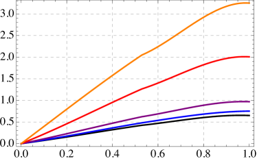
Figure 10: The curves correspond, from bottom to top, to $a/T=0,\,4.41,\,12.2,\,86,\,249$.

Appendix B Limiting regimes

The background geometry is known analytically in the limiting regimes of low and high temperature ALT ; MT2 . This allows to obtain analytic results for the branes’ embeddings in these limits, which we do next.

B.1 Zero temperature limit

We start by studying the D7-branes’ behavior at exactly zero temperature. The solution for the metric (in string frame) is given by eq. (2.16) of ALT

$$ds^{2}=\tilde{R}{{}^{2}_{s}}\left(\tilde{r}^{7/3}(-dt^{2}+dx^{2}+dy^{2})+\tilde{r}^{5/3}dz^{2}+\frac{d\tilde{r}^{2}}{\tilde{r}^{5/3}}+\frac{12}{11}\tilde{r}^{1/3}d\Omega{{}^{2}_{5}}\right).$$ (71)

The $\rho$ coordinate is defined so that

$$\frac{d\tilde{r}^{2}}{\tilde{r}^{5/3}}+\frac{12}{11}\tilde{r}^{1/3}d\Omega{{}^{2}_{5}}\propto d\rho^{2}+\rho^{2}d\Omega{{}^{2}_{5}}.$$ (72)

The condition to get this is

$$\frac{12}{11}\frac{\tilde{r}^{1/3}}{\rho^{2}}=\frac{1}{\tilde{r}^{5/3}}\left(\frac{d\tilde{r}}{d\rho}\right)^{2},$$ (73)

which leads to

$$\tilde{r}=\rho^{\sqrt{\frac{12}{11}}}.$$ (74)

Under this change of coordinates, the metric (71) becomes

$$\frac{ds^{2}}{\tilde{R}{{}^{2}_{s}}}=\rho^{\frac{14}{\sqrt{33}}}\left(-dt^{2}+dx^{2}+dy^{2}\right)+\rho^{\frac{10}{\sqrt{33}}}dz^{2}+\frac{12}{11}\rho^{2\left(\frac{1}{\sqrt{33}}-1\right)}\left(d\rho^{2}+\rho^{2}d\Omega{{}^{2}_{5}}\right).$$ (75)

The induced metric on the D7-branes is obtained by replacing

$$d\rho^{2}+\rho^{2}d\Omega{{}^{2}_{5}}\rightarrow\left(1+\dot{R}^{2}\right)dr^{2}+r^{2}d\Omega{{}^{2}_{3}},$$ (76)

where, as in the main text, $\rho^{2}={R(r)}^{2}+r^{2}$. The determinant of this metric is

$$\sqrt{-g}=\rho^{10\sqrt{\frac{3}{11}}-4}r^{3}\sqrt{1+\dot{R}^{2}},$$ (77)

which, together with the solution for the dilaton specified in (2.14) of ALT

$$\phi=\frac{2}{3}\log\tilde{r}+\phi_{0},$$ (78)

leads to the Lagrangian

$$\mathcal{L}\propto\left(r^{2}+R^{2}\right)^{\frac{n}{2}}r^{3}\sqrt{1+\dot{R}^{2}}\,,$$ (79)

where $n=26/\sqrt{33}-4$. The equation of motion for $R(r)$ is found to be

$$n\left(r^{2}+R^{2}\right)^{\frac{n-2}{2}}Rr^{3}\sqrt{1+\dot{R}^{2}}=\partial_{r}\left(\left(r^{2}+R^{2}\right)^{\frac{n}{2}}r^{3}\frac{\dot{R}}{\sqrt{1+\dot{R}^{2}}}\right),$$ (80)

whose solution near $r=0$ is given by

$$R(r)=R_{0}+\frac{n}{8R_{0}}r^{2}+{\cal O}(r^{4}).$$ (81)

This displays a positive curvature, showing that the anisotropy has the effect of bending the branes downward even in the absence of a black hole.

B.2 High temperature

We now discuss the case of small values of the anisotropy parameter or, equivalently, of high temperature. In this limit, the expressions for the background fields have been previously calculated in MT2 and are given by

$$\phi(u) = -\frac{1}{4}\ln\left(1+u^{2}\right)a^{2}+{\cal O}\left(a^{4}\right)\,,$$ (82)

$${\cal F}(u) = \left(1-u^{4}\right)+\left(\frac{u^{2}}{3}-\left(\frac{1}{3}+\frac{5\ln 2}{12}\right)u^{4}+\frac{1}{8}\left(1+\frac{7}{3}u^{4}\right)\ln\left(1+u^{2}\right)\right)a^{2}+{\cal O}\left(a^{4}\right)\,,$$ (83)

$${\cal B}(u) = -\frac{1}{4}\ln\left(1+u^{2}\right)a^{2}+{\cal O}\left(a^{4}\right)\,.$$ (84)

Using (14), one can derive

$$u(\rho)=\frac{\sqrt{2}\rho}{\sqrt{1+\rho^{4}}}-\rho\frac{2\rho^{2}-\left(1+\rho^{4}\right)\left(1-\ln 32+10\ln(1+\rho^{2})-5\ln(1+\rho^{4})\right)}{24\sqrt{2}{(1+\rho^{4})}^{3/2}}a^{2}+{\cal O}\left(a^{4}\right)\,.$$ (85)

Inserting this change of coordinates into the expressions above, one can directly derive expressions for the fields to lowest order in $a$. The function $P(\rho)$ defined in (20) takes the form

$$P(\rho) = \frac{1}{4}\left(1-\frac{1}{\rho^{8}}\right)$$ (89)

$$+\frac{1-\rho^{2}+\rho^{6}-5\ln 2+\rho^{8}(\ln 32-1)-6(\rho^{8}-1)\ln(\rho^{2}+1)+3(\rho^{8}-1)\ln(\rho^{4}+1)}{48\rho^{8}}a^{2}$$

$$+{\cal O}\left(a^{4}\right)\,.$$

This is a lengthy expression and, as a consequence, the perturbation introduced by $a\neq 0$ is too complicated to be dealt with analytically. However, a near-horizon approximation gives a solution for the embedding of the form

$$\psi(\rho)=\psi^{(0)}(\rho)+\frac{1}{32}\psi_{\textrm{\tiny H}}\left(\rho-1\right)^{4}a^{2}+{\cal O}\left(a^{4},{(\rho-1)}^{5}\right),$$ (90)

where $\psi^{(0)}(\rho)$ is the isotropic solution.

Appendix C Expansion of the divergent action

In this appendix, we derive the expressions (43)-(LABEL:phi_det) used in Sec. 4.1. We start by recalling the general FG expansions of the fields reviewHR

$$g_{ij} = {g_{(0)}}_{ij}+{g_{(2)}}_{ij}v^{2}+\left({g_{(4)}}_{ij}+{h_{(4)}}_{ij}\log{v}\right)v^{4}+\mathcal{O}\left(v^{6}\right),$$ (91)

$$\phi = \phi_{(0)}+\phi_{(2)}v^{2}+\left(\phi_{(4)}+\tilde{\phi}_{(4)}\log{v}\right)v^{4}+\mathcal{O}\left(v^{6}\right),$$ (92)

$$\psi = \psi_{(0)}v+\left(\psi_{(2)}+\tilde{\psi}_{(2)}\log{v}\right)v^{3}+\mathcal{O}\left(v^{5}\right).$$ (93)

The axion has a constant profile in the radial direction, so that $\chi=\chi_{(0)}$.

With some algebra, it is possible to see that the coefficients of the divergences in (LABEL:divergences) are given by the following combinations of the asymptotic expansions of the fields

$$a_{(0)} = \frac{1}{4},$$ (94)

$$a_{(1)} = \frac{1}{4}\left({g_{(0)}}^{ij}{g_{(2)}}_{ij}+2\phi_{(2)}-2\psi_{(0)}^{2}\right),$$ (95)

$$a_{(2)} = -\frac{1}{2}{g_{(0)}}^{ij}{g_{(4)}}_{ij}-\frac{1}{8}({g_{(0)}}^{ij}{g_{(2)}}_{ij})^{2}+\frac{1}{4}{g_{(0)}}^{ij}{g_{(2)}}_{jk}{g_{(0)}}^{kl}{g_{(2)}}_{li}$$ (97)

$$-\frac{1}{2}\phi_{(2)}{g_{(0)}}^{ij}{g_{(2)}}_{ij}-\frac{1}{2}\phi_{(2)}^{2}+\frac{1}{2}\psi_{(0)}^{2}{g_{(0)}}^{ij}{g_{(2)}}_{ij}+\phi_{(2)}\psi_{(0)}^{2}-\psi_{(0)}\tilde{\psi}_{(2)},$$

$$a_{(3)} = -\frac{1}{4}\left({g_{(0)}}^{ij}{h_{(4)}}_{ij}+2\tilde{\phi}_{(4)}\right).$$ (98)

These terms in the FG expansion of the fields obey certain equations of motion given by Yiannis

$${g_{(2)}}_{ij}=\frac{e^{2\phi_{(0)}}}{4}\left(\partial_{i}\chi_{(0)}\partial_{j}\chi_{(0)}-\frac{1}{6}{g_{(0)}}_{ij}{g_{(0)}}^{kl}\partial_{k}\chi_{(0)}\partial_{l}\chi_{(0)}\right),$$ (99)

$${h_{(4)}}_{ij}=\frac{e^{4\phi_{(0)}}}{6}{g_{(0)}}^{kl}\partial_{k}\chi_{(0)}\partial_{l}\chi_{(0)}\left(\partial_{i}\chi_{(0)}\partial_{j}\chi_{(0)}-\frac{1}{4}{g_{(0)}}_{ij}{g_{(0)}}^{ab}\partial_{a}\chi_{(0)}\partial_{b}\chi_{(0)}\right),$$ (100)

$${g_{(0)}}^{ij}{g_{(4)}}_{ij}=-\frac{11e^{4\phi_{(0)}}}{576}({g_{(0)}}^{ij}\partial_{i}\chi_{(0)}\partial_{j}\chi_{(0)})^{2},$$ (101)

$$\phi_{(2)}=-\frac{e^{2\phi_{(0)}}}{4}{g_{(0)}}^{ij}\partial_{i}\chi_{(0)}\partial_{j}\chi_{(0)},$$ (102)

$$\tilde{\phi}_{(4)}=-\frac{e^{4\phi_{(0)}}}{6}({g_{(0)}}^{ij}\partial_{i}\chi_{(0)}\partial_{j}\chi_{(0)})^{2},$$ (103)

$$\tilde{\psi}_{(2)}=-\psi_{(0)}\left(\phi_{(2)}+\frac{1}{2}{g_{(0)}}^{ij}{g_{(2)}}_{ij}\right).$$ (104)

Moreover, one can check that

$${g_{(0)}}^{ij}{g_{(2)}}_{ij}=\frac{e^{2\phi_{(0)}}}{12}{g_{(0)}}^{ij}\partial_{i}\chi_{(0)}\partial_{j}\chi_{(0)}\,,\qquad{g_{(0)}}^{ij}{h_{(4)}}_{ij}=0\,,$$ (105)

$${g_{(0)}}^{ij}{g_{(2)}}_{jk}{g_{(0)}}^{kl}{g_{(2)}}_{li}=\frac{7e^{4\phi_{(0)}}}{144}({g_{(0)}}^{ij}\partial_{i}\chi_{(0)}\partial_{j}\chi_{(0)})^{2}\,.$$ (106)

These are all the ingredients needed to invert the expansions. To zero-th order in $v$ we have from (93) that

$${g_{(0)}}_{ij}=g_{ij},\hskip 28.45274pt\phi_{(0)}=\phi,\hskip 28.45274pt\chi_{(0)}=\chi,\hskip 28.45274pt\psi_{(0)}=\frac{\psi}{v}.$$ (107)

Substituting this in (101)-(106) and taking into consideration that $g_{ij}=v^{2}\gamma_{ij}$ leads to

$${g_{(0)}}^{ij}{g_{(2)}}_{ij}=\frac{e^{2\phi}}{12v^{2}}\partial^{i}\chi\partial_{i}\chi\,,\qquad{g_{(0)}}^{ij}{g_{(4)}}_{ij}=-\frac{11e^{4\phi}}{576v^{4}}(\partial^{i}\chi\partial_{i}\chi)^{2},$$ (108)

$${g_{(0)}}^{ij}{g_{(2)}}_{jk}{g_{(0)}}^{kl}{g_{(2)}}_{li}=\frac{7e^{4\phi}}{144v^{4}}(\partial^{i}\chi\partial_{i}\chi)^{2}\,,$$ (109)

$$\phi_{(2)}=-\frac{e^{2\phi}}{4v^{2}}\partial^{i}\chi\partial_{i}\chi\,,\qquad\tilde{\phi}_{(4)}=-\frac{e^{4\phi}}{6v^{4}}(\partial^{i}\chi\partial_{i}\chi)^{2},$$ (110)

$$\psi_{(0)}=\frac{1}{v}\psi\left(1-\frac{5e^{2\phi}}{24}\partial^{i}\chi\partial_{i}\chi\log{v}\right)\,,\qquad\tilde{\psi}_{(2)}=\frac{5e^{2\phi}}{24v^{3}}\psi\,\partial^{i}\chi\partial_{i}\chi\,,$$ (111)

and, similarly, to

$$\sqrt{-g_{(0)}}=v^{4}\sqrt{-\gamma}\left(1-\frac{e^{2\phi}}{24}\partial^{i}\chi\partial_{i}\chi\right),$$ (112)

$$e^{\phi_{(0)}}=e^{\phi}\left(1+\frac{e^{2\phi}}{4}\partial^{i}\chi\partial_{i}\chi+\frac{e^{4\phi}}{6}\left(\partial^{i}\chi\partial_{i}\chi\right)^{2}\log{v}\right).$$ (113)

Using these expressions, (43)-(LABEL:phi_det) can be obtained readily.

References

• (1) J. M.  Maldacena, “The large $N$ limit of superconformal field theories and supergravity,” Adv. Theor. Math. Phys. 2, 231 (1998) [Int. J. Theor. Phys. 38, 1113 (1999)] [hep-th/9711200]; S. S. Gubser, I. R. Klebanov, A. M. Polyakov, “Gauge theory correlators from noncritical string theory,” Phys. Lett.  B428, 105-114 (1998) [hep-th/9802109]; E. Witten, “Anti-de Sitter space and holography,” Adv. Theor. Math. Phys.  2, 253-291 (1998) [hep-th/9802150].
• (2) A. Karch and L. Randall, “Open and closed string interpretation of SUSY CFT’s on branes with boundaries,” JHEP 0106, 063 (2001) [hep-th/0105132]; A. Karch and E. Katz, “Adding flavor to AdS / CFT,” JHEP 0206, 043 (2002) [hep-th/0205236].
• (3) D. Mateos, R. C. Myers and R. M. Thomson, “Holographic phase transitions with fundamental matter,” Phys. Rev. Lett.  97, 091601 (2006) [hep-th/0605046]; “Thermodynamics of the brane,” JHEP 0705, 067 (2007) [hep-th/0701132].
• (4) R. C. Myers, A. O. Starinets and R. M. Thomson, “Holographic spectral functions and diffusion constants for fundamental matter,” JHEP 0711, 091 (2007) [arXiv:0706.0162 [hep-th]]; A. Karch and A. O’Bannon, “Holographic thermodynamics at finite baryon density: Some exact results,” JHEP 0711, 074 (2007) [arXiv:0709.0570 [hep-th]]; D. Mateos, S. Matsuura, R. C. Myers and R. M. Thomson, “Holographic phase transitions at finite chemical potential,” JHEP 0711, 085 (2007) [arXiv:0709.1225 [hep-th]]; T. Albash, V. G. Filev, C. V. Johnson and A. Kundu, “Finite temperature large N gauge theory with quarks in an external magnetic field,” JHEP 0807, 080 (2008) [arXiv:0709.1547 [hep-th]]; F. Bigazzi, A. L. Cotrone, J. Mas, A. Paredes, A. V. Ramallo and J. Tarrio, “D3-D7 Quark-Gluon Plasmas,” JHEP 0911, 117 (2009) [arXiv:0909.2865 [hep-th]]; C. Nunez, A. Paredes and A. V. Ramallo, “Unquenched Flavor in the Gauge/Gravity Correspondence,” Adv. High Energy Phys.  2010, 196714 (2010) [arXiv:1002.1088 [hep-th]].
• (5) J. Erdmenger, N. Evans, I. Kirsch and E. Threlfall, “Mesons in Gauge/Gravity Duals - A Review,” Eur. Phys. J. A 35, 81 (2008) [arXiv:0711.4467 [hep-th]].
• (6) J. Adams et al. [STAR Collaboration], “Experimental and theoretical challenges in the search for the quark gluon plasma: The STAR collaboration’s critical assessment of the evidence from RHIC collisions,” Nucl. Phys.  A 757, 102 (2005) [arXiv:nucl-ex/0501009]; K. Adcox et al. [PHENIX Collaboration], “Formation of dense partonic matter in relativistic nucleus nucleus collisions at RHIC: Experimental evaluation by the PHENIX collaboration,” Nucl. Phys.  A 757, 184 (2005) [arXiv:nucl-ex/0410003]; Proceedings of Quark Matter 2011: J. Phys. GG 38, number 12 (December 2011).
• (7) E. Shuryak, “Why does the quark gluon plasma at RHIC behave as a nearly ideal fluid?,” Prog. Part. Nucl. Phys.  53, 273 (2004) [arXiv:hep-ph/0312227]; “What RHIC experiments and theory tell us about properties of quark-gluon plasma?,” Nucl. Phys.  A 750, 64 (2005) [arXiv:hep-ph/0405066].
• (8) J. Casalderrey-Solana, H. Liu, D. Mateos, K. Rajagopal and U. A. Wiedemann, “Gauge/String Duality, Hot QCD and Heavy Ion Collisions,” arXiv:1101.0618 [hep-th].
• (9) R. C. Myers and S. E. Vazquez, “Quark Soup al dente: Applied Superstring Theory,” Class. Quant. Grav.  25, 114008 (2008) [arXiv:0804.2423 [hep-th]].
• (10) J. Y. Ollitrault, “Anisotropy as a signature of transverse collective flow,” Phys. Rev. D 46, 229 (1992).
• (11) D. Mateos and D. Trancanelli, “The anisotropic N=4 super Yang-Mills plasma and its instabilities,” Phys. Rev. Lett.  107, 101601 (2011) [arXiv:1105.3472 [hep-th]].
• (12) D. Mateos and D. Trancanelli, “Thermodynamics and Instabilities of a Strongly Coupled Anisotropic Plasma,” JHEP 1107, 054 (2011) [arXiv:1106.1637 [hep-th]].
• (13) T. Azeyanagi, W. Li and T. Takayanagi, “On String Theory Duals of Lifshitz-like Fixed Points,” JHEP 0906, 084 (2009) [arXiv:0905.0688 [hep-th]].
• (14) A. Rebhan and D. Steineder, “Violation of the Holographic Viscosity Bound in a Strongly Coupled Anisotropic Plasma,” Phys. Rev. Lett.  108, 021601 (2012) [arXiv:1110.6825 [hep-th]]; M. Chernicoff, D. Fernandez, D. Mateos and D. Trancanelli, “Drag force in a strongly coupled anisotropic plasma,” JHEP 1208, 100 (2012) [arXiv:1202.3696 [hep-th]]; D. Giataganas, “Probing strongly coupled anisotropic plasma,” JHEP 1207, 031 (2012) [arXiv:1202.4436 [hep-th]]; M. Chernicoff, D. Fernandez, D. Mateos and D. Trancanelli, “Jet quenching in a strongly coupled anisotropic plasma,” JHEP 1208, 041 (2012) [arXiv:1203.0561 [hep-th]]; K. A. Mamo, “Holographic Wilsonian RG Flow of the Shear Viscosity to Entropy Ratio in Strongly Coupled Anisotropic Plasma,” JHEP 1210, 070 (2012) [arXiv:1205.1797 [hep-th]]; A. Rebhan and D. Steineder, “Probing Two Holographic Models of Strongly Coupled Anisotropic Plasma,” JHEP 1208, 020 (2012) [arXiv:1205.4684 [hep-th]]; K. B. Fadafan and H. Soltanpanahi, “Energy loss in a strongly coupled anisotropic plasma,” JHEP 1210, 085 (2012) [arXiv:1206.2271 [hep-th]]; B. Muller and D. -L. Yan, “Light Probes in a Strongly Coupled Anisotropic Plasma,” Phys. Rev. D 87, 046004 (2013) [arXiv:1210.2095 [hep-th]]; L. Patiño and D. Trancanelli, “Thermal photon production in a strongly coupled anisotropic plasma,” JHEP 1302, 154 (2013) [arXiv:1211.2199 [hep-th]]; S. Chakraborty and N. Haque, “Holographic quark-antiquark potential in hot, anisotropic Yang-Mills plasma,” Nucl. Phys. B 874, 821 (2013) [arXiv:1212.2769 [hep-th]]; D. Giataganas, “Observables in Strongly Coupled Anisotropic Theories,” PoS Corfu 2012, 122 (2013) [arXiv:1306.1404 [hep-th]]; K. B. Fadafan, D. Giataganas and H. Soltanpanahi, “The Imaginary Part of the Static Potential in Strongly Coupled Anisotropic Plasma,” JHEP 1311, 107 (2013) [arXiv:1306.2929 [hep-th]]; G. Arciniega, P. Ortega and L. Patiño, “Brighter Branes, enhancement of photon production by strong magnetic fields in the gauge/gravity correspondence,” JHEP 1404, 192 (2014) [arXiv:1307.1153 [hep-th]]; M. Ali-Akbari and H. Ebrahim, “Chiral Symmetry Breaking: To Probe Anisotropy and Magnetic Field in QGP,” Phys. Rev. D 89, no. 6, 065029 (2014) [arXiv:1309.4715 [hep-th]]; D. Giataganas and H. Soltanpanahi, “Universal properties of the Langevin diffusion coefficients,” Phys. Rev. D 89, 026011 (2014) [arXiv:1310.6725 [hep-th]]; S. Chakrabortty, S. Chakraborty and N. Haque, “Brownian motion in strongly coupled, anisotropic Yang-Mills plasma: A holographic approach,” Phys. Rev. D 89, 066013 (2014) [arXiv:1311.5023 [hep-th]]; D. Giataganas and H. Soltanpanahi, “Heavy Quark Diffusion in Strongly Coupled Anisotropic Plasmas,” JHEP 1406, 047 (2014) [arXiv:1312.7474 [hep-th]]; L. Cheng, X. H. Ge and S. J. Sin, “Anisotropic plasma with a chemical potential and scheme-independent instabilities,” Phys. Lett. B 734, 116 (2014) [arXiv:1404.1994 [hep-th]]; L. Cheng, X. H. Ge and S. J. Sin, “Anisotropic plasma at finite $U(1)$ chemical potential,” JHEP 1407, 083 (2014) [arXiv:1404.5027 [hep-th]].
• (15) E. Banks and J. P. Gauntlett, “A new phase for the anisotropic N=4 super Yang-Mills plasma,” JHEP 1509, 126 (2015) [arXiv:1506.07176 [hep-th]]; E. Banks, “Phase transitions of an anisotropic N=4 super Yang-Mills plasma via holography,” arXiv:1604.03552 [hep-th].
• (16) M. Chernicoff, D. Fernandez, D. Mateos and D. Trancanelli, “Quarkonium dissociation by anisotropy,” JHEP 1301, 170 (2013) [arXiv:1208.2672 [hep-th]].
• (17) K. Skenderis, “Lecture notes on holographic renormalization,” Class. Quant. Grav.  19, 5849 (2002) [hep-th/0209067].
• (18) A. Karch, A. O’Bannon and K. Skenderis, “Holographic renormalization of probe D-branes in AdS/CFT,” JHEP 0604, 015 (2006) [hep-th/0512125].
• (19) V. Jahnke, A. Luna, L. Patiño and D. Trancanelli, “More on thermal probes of a strongly coupled anisotropic plasma,” JHEP 1401, 149 (2014) [arXiv:1311.5513 [hep-th]].
• (20) M. Gell-Mann, R. J. Oakes and B. Renner, “Behavior of current divergences under SU(3) x SU(3),” Phys. Rev.  175, 2195 (1968).
• (21) M. Kruczenski, D. Mateos, R. C. Myers and D. J. Winters, “Meson spectroscopy in AdS / CFT with flavor,” JHEP 0307, 049 (2003) [hep-th/0304032].
• (22) A. Karch, A. O’Bannon and L. G. Yaffe, “Critical Exponents from AdS/CFT with Flavor,” JHEP 0909, 042 (2009) [arXiv:0906.4959 [hep-th]].
• (23) B. B. Abelev et al. [ALICE Collaboration], “Centrality, rapidity and transverse momentum dependence of $J/\psi$ suppression in Pb-Pb collisions at $\sqrt{s_{\rm NN}}$=2.76 TeV,” Phys. Lett. B 734, 314 (2014) [arXiv:1311.0214 [nucl-ex]].
• (24) I. Papadimitriou, “Holographic Renormalization of general dilaton-axion gravity,” JHEP 1108, 119 (2011) [arXiv:1106.4826 [hep-th]].