Motion of solitons in one-dimensional spin-orbit-coupled Bose-Einstein condensates

Abstract

Solitons play a fundamental role in dynamics of nonlinear excitations. Here we explore the motion of solitons in one-dimensional uniform Bose-Einstein condensates subjected to a spin-orbit coupling (SOC). We demonstrate that the spin dynamics of solitons is governed by a nonlinear Bloch equation. The spin dynamics influences the orbital motion of the solitons leading to the spin-orbit effects in the dynamics of the macroscopic quantum objects (mean-field solitons). The latter perform oscillations with a frequency determined by the SOC, Raman coupling, and intrinsic nonlinearity. These findings reveal unique features of solitons affected by the SOC, which is confirmed by analytical considerations and numerical simulations of the underlying Gross-Pitaevskii equations.

Solitons, which are generally realized as self-supported solitary waves, are among the most fundamental objects in the nonlinear science. With the realization of Bose-Einstein condensates (BEC), matter-wave solitons have drawn enormous interest Randy ; Brazh ; Fatkh ; Morsch ; fsm ; soliton1 ; Dim ; RMP2 ; vs . In the experiments, both bright and dark solitons have been successively created in atomic BEC Randy ; bs1 ; soliton2 ; soliton3 ; soliton4 ; soliton5 . On the other hand, the successful realization of the artificial spin-orbit coupling (SOC) in binary BEC soc1 ; soc2 ; soc3 ; soc4 has stimulated intensive studies on novel SOC-induced effects Zhaih ; TLHo ; Lyou ; CWZhang1 ; YLi ; SZhang ; HHu ; CWZhang2 ; ZQYu ; CWZhang3 ; CWZhang4 ; WYi ; Galitski2013 ; Goldman2014 ; Zhai2015 ; Su2016 . In particular, a variety of solitons species, such as stripe modes, 2D composite solitons, and half-vortex gap soliton have been predicted in the condensates combining the SOC, which is a linear interaction, and the intrinsic collisional nonlinearity ss1 ; ss4 ; ss3 ; ss2 ; ss5 ; ss6 ; ss7 ; ss8 ; ss9 ; bdd ; sgs ; 2cs1 ; Luca ; 2cs2 ; hvgs ; Petra ; YCZhang ; Fialko .

Soliton dynamics has been the subject of many studies carried out in various settings, including BEC Randy ; Brazh ; Fatkh ; Morsch ; fsm ; soliton1 ; Dim ; RMP2 ; vs , nonlinear optics RMP1 ; KivPel ; KA ; bullets ; DesTorKiv ; Dum ; PT , and others. In particular, it has been shown that harmonic trapping potentials induce motion of solitons in quasi-one-dimensional (1D) BEC d10 ; d9 ; d7 ; d11 ; HPu ; d12 . Due to the particle-like nature, the soliton dynamics differs essentially from the dipole mode of the non-interacting condensate loaded into the same potential. In particular, the oscillation frequency of trapped dark solitons differs by factor $1/\sqrt{2}$ from the trap frequency d10 . Here, we address the soliton dynamics in 1D BEC under the action of the Raman-induced SOC soc1 ; soc2 . Since the Raman transition can flip the spin along with inducing a finite momentum transfer, the evolution of the spin degree of freedom may be coupled to the spatial motion of solitons. This effect, if it can be made conspicuous enough, may be considered as the SOC at the level of the motion of a macroscopic quantum body, the matter-wave soliton. In this connection, it is relevant to mention a recent result showing that the SOC can induce anharmonic properties beyond the effective-mass approximation in collective dipole oscillations soc2 ; ChenZ ; LiY . Yet the macroscopic SOC effects in the motion of solitons have not been explored before, to the best of our knowledge.

In this work we investigate the soliton dynamics in 1D uniform BEC influenced by the SOC. We find that an interplay of the SOC, Raman coupling, and nonlinearity induces precession of the soliton’s spin $\mathbf{S}$ under the action of an effective magnetic field, which is governed by a nonlinear Bloch equation (12). In turn, the spin precession couples to the orbital motion of the soliton via feedback onto its center-of-mass momentum, as shown below by equation of motion (15) for the center-of-mass coordinate, $\left\langle z\right\rangle$. Thus, Eqs. (12) and (15) directly demonstrate the effects of the SOC on the 1D motion of the macroscopic quantum object.

In the presence of SOC, the dynamics of the quasi-1D BEC, elongated in the direction of $z$, is modelled by the mean-field Gross-Pitaevskii (GP) equation:

$$i\partial_{t}\left(\!\begin{array}[]{c}\psi_{\uparrow}\\ \psi_{\downarrow}\end{array}\!\right)\!=\!\hat{h}_{0}\left(\!\begin{array}[]{c}\psi_{\uparrow}\\ \psi_{\downarrow}\end{array}\!\right)\!+\!\left(\begin{array}[]{c}g_{\uparrow\uparrow}|\psi_{\uparrow}|^{2},g_{\uparrow\downarrow}|\psi_{\downarrow}|^{2}\\ g_{\downarrow\uparrow}|\psi_{\uparrow}|^{2},g_{\downarrow\downarrow}|\psi_{\downarrow}|^{2}\end{array}\right)\!\left(\!\begin{array}[]{c}\psi_{\uparrow}\\ \psi_{\downarrow}\end{array}\!\right),$$ (1)

where $\psi_{\sigma}$ are the pseudo-spin components of the BEC macroscopic wave function, with $\sigma=\uparrow,\downarrow$ labelling the spin states. These can represent, for instance, the hyperfine states $|1,-1\rangle$ and $|1,0\rangle$ of ⁸⁷Rb atoms soc1 . Here

$$\hat{h}_{0}=-\frac{1}{2}\partial_{z}^{2}+V(z)+i\lambda\partial_{z}\sigma_{z}+\Omega\sigma_{x}+\delta\sigma_{z}$$ (2)

is a single-particle Hamiltonian which includes the Raman-induced SOC characterized by a strength $\lambda$, with $\Omega$ and $\delta$ describing, respectively, the frequencies of the Raman coupling and the Zeeman detuning. Here also $V(z)=\gamma^{2}z^{2}/2$ is an effective 1D harmonic trap potential, and $\gamma\equiv\omega_{z}/\omega_{\bot}$ is the trap’s aspect ratio, with $\omega_{z}$ and $\omega_{\bot}$ being the trapping frequencies along the longitudinal and transverse directions, respectively. The frequencies and lengths are measured in units $\omega_{\bot}$ and $a_{\bot}=\sqrt{\hbar/m\omega_{\bot}}$, respectively, and, as mentioned above, $\lambda=k_{L}a_{\bot}$ represents the SOC strength, with $k_{L}$ being the momentum transfer. Note that, as the strengths of the inter- and intra-species atomic interactions are very close in the experiment, it is reasonable to assume $SU(2)$-symmetric spin interactions, with all components $g_{\sigma\sigma^{\prime}}$ taking a single value, $g$. To focus on the SOC effects on the dynamics of solitons, we first consider the free space, while the external trap will be discussed afterwards.

For $\lambda=\Omega=0$, the system reduces to a normal binary BEC without the SOC. In this case, Eq. (1) is known as the integrable Manakov’s system which gives rise to well-known exact soliton solutions manakov . In particular,bright-bright (BB) solitons are $\psi_{\sigma}=\left(\eta\epsilon_{\sigma}/\sqrt{-g}\right)$sech$\left(\eta z\right)\exp\left(i\eta^{2}t/2\right)$ for the attractive sign of the nonlinearity, $g<0$, where $\eta^{-1}$ is the soliton’s width and $\epsilon_{\sigma}$ satisfies the normalized condition, $|\epsilon_{\uparrow}|^{2}+|\epsilon_{\downarrow}|^{2}=-g/(2\eta)$. We use such exact soliton solutions as an initially prepared wave function, and then study the soliton dynamics as the SOC is switched on. Note that Eq. (2) is an effective single-particle Hamiltonian in the frame transformed via the local pseudo-spin rotation by angle $\vartheta=2\lambda z$ about the $z$ axis soc1 ; soc2 . The transformation adds opposite phase factors, $e^{\pm i\lambda z}$, to the two components of the input waveforms.

In the general case, the GP system (1) is no longer integrable. Therefore we employ a variational approximation to investigate the soliton dynamics Progress ; fsm , based on Lagrangian $L(t)=\int_{-\infty}^{+\infty}\{(i/2)\sum_{\sigma=\uparrow,\downarrow}\left[\psi_{\sigma}^{\ast}\left(\psi_{\sigma}\right)_{t}-\psi_{\sigma}\left(\psi_{\sigma}^{\ast}\right)_{t}\right]-\mathcal{H}\}dz$, where $\mathcal{H}$ is the Hamiltonian density of the system. We first consider the attractive nonlinearity, with $g<0$. In this case, we introduce the following variational Ansatz for BB solitons, with the total norm fixed to be $1$:

$$\left(\begin{array}[]{c}\psi_{\uparrow}\\ \psi_{\downarrow}\end{array}\right)=\sqrt{\frac{\eta}{2}}\left(\begin{array}[]{c}\left(\sin\theta\right)\>\text{sech}(\eta z+\xi_{\uparrow})e^{i\left(k_{\uparrow}z+\varphi_{\uparrow}\right)}\\ \left(\cos\theta\right)\>\text{sech}(\eta z+\xi_{\downarrow})e^{i\left(k_{\downarrow}z+\varphi_{\downarrow}\right)}\end{array}\right)\,,$$ (3)

where $\theta$, $\eta$, $\xi_{\sigma}$, $k_{\sigma}$, $\varphi_{\sigma}$ are time-dependent variational parameters. Here $\theta$ determines the population imbalance between the pseudo-spin components, $\eta^{-1}$ defines their common width, $k_{\sigma}$ is the wavenumber, and $\varphi_{\sigma}$ the phase. For the $SU(2)$ atomic interactions, two-component solitons favor the mixed phase phasemixing . Hence the positions of spin up and down solitons will overlap, $\xi_{\uparrow}=\xi_{\downarrow}=\xi$, as confirmed by the numerical simulations below.

Inserting the Ansatz (3) into the Lagrangian and performing the integration, we obtain

$$L\left(t\right) = \frac{\xi}{\eta}\frac{dk_{+}}{dt}-\frac{\xi}{\eta}\cos\left(2\theta\right)\frac{dk_{-}}{dt}-\frac{d\varphi_{+}}{dt}+\cos\left(2\theta\right)\frac{d\varphi_{-}}{dt}$$ (4)

$$- \frac{1}{2}\left[k_{+}^{2}-2k_{+}k_{-}\cos\left(2\theta\right)+k_{-}^{2}\right]-\frac{1}{6}\eta^{2}-\frac{1}{6}g\eta$$

$$- \frac{\Omega\pi k_{-}\sin(2\theta)\cos\left(2\varphi_{-}-2k_{-}\xi/\eta\right)}{\eta\sinh\left(\pi k_{-}/\eta\right)}$$

$$+ \delta\cos\left(2\theta\right)-\lambda\left[k_{+}\cos\left(2\theta\right)-k_{-}\right]\,,$$

where $k_{\pm}\equiv\left(1/2\right)(k_{\uparrow}\pm k_{\downarrow})$ and $\varphi_{\pm}\equiv\left(1/2\right)(\varphi_{\uparrow}\pm\varphi_{\downarrow})$. The evolution of the variational parameters is governed by the corresponding Euler-Lagrangian (EL) equations, see the Supplementary material for details.

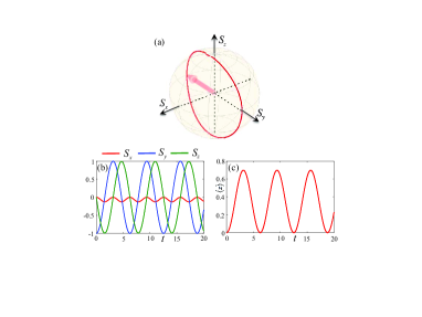
Figure 1: (Color online). The track of the spin density on the Bloch sphere (a), and the corresponding evolution of the spin components (b) and center-of-mass coordinate (c) of the soliton for the initially balanced state, with $\theta(t=0)=\pi/{4}$, and initial phase difference $\varphi_{-}(t=0)=\pi/4$ [see Eq. (3)]. Other parameters are $\Omega=0.5$, $\lambda=0.5\sqrt{\Omega}$, $\delta=0$, and $g=-10$.

Note that the EL equations produce simple results, $\eta\approx-g/2$ and $k_{-}\approx\lambda$, in the case of a weak SOC, $\pi\lambda<<\eta$. Indeed, in the absence of SOC, the relation $\eta=-g/2$ holds for the normalized wave function, indicating that the width of the solitons is determined by the nonlinearity, and $k_{-}$ remains equal to the initial relative momentum $\lambda$ between the components of the soliton. Thus, we arrive at a reduced system of the EL equations, in which $\eta$ and $k_{-}$ are considered as frozen quantities:

$$\dot{k}_{+} = 2\lambda\tilde{\Omega}\sin({2\theta})\sin{\phi}\,,$$ (5)

$$\dot{\phi} = -2\tilde{\Omega}\cot(2\theta)\cos\phi+2\lambda k_{+}-2\delta\,,$$ (6)

$$\dot{\theta} = -\tilde{\Omega}\sin\phi\,,$$ (7)

$$\dot{\langle z\rangle} = k_{+}\,.$$ (8)

Here, $\left\langle z\right\rangle=\int_{-\infty}^{+\infty}z(|\psi_{\uparrow}|^{2}+|\psi_{\downarrow}|^{2})dz\equiv-\xi/\eta$ is the center-of-mass coordinate, $\tilde{\Omega}\equiv\Omega\pi\left(\lambda/\eta\right)\sinh\left(\pi\lambda/\eta\right)$, and $\phi\equiv 2\varphi_{-}+2k_{-}\langle z\rangle$ is the phase difference between the two components of the soliton. Thus, Eqs. (5)-(8) account for the nonlinear coupling of the center-of-mass momentum $k_{+}$, phase difference $\phi$, population imbalance $\theta$, and center-of-mass coordinate ${\langle z\rangle}$.

We introduce a normalized complex-valued spinor, $\mathbf{\chi}=(\chi_{\uparrow},\chi_{\downarrow})$ describing the two-component wave function $\psi_{\sigma}=\sqrt{\rho\left(z,t\right)}\chi_{\sigma}$, where $\rho\equiv|\psi_{\uparrow}|^{2}+|\psi_{\downarrow}|^{2}$ is the total density, with $\left|\chi_{\uparrow}\right|^{2}+\left|\chi_{\downarrow}\right|^{2}=1$. Furthermore we define the spin density $\mathbf{S}=\mathbf{\chi}^{T}\mathbf{\sigma\chi}$, where $\mathbf{\sigma\equiv}\left\{\sigma_{x},\sigma_{y},\sigma_{z}\right\}$ is a vector set of the Pauli matrices, we have $\{S_{x},S_{y},S_{z}\}=\{\sin(2\theta)\cos(2\lambda z+2\varphi_{-}),$$-\sin(2\theta)\sin(2\lambda z+2\varphi_{-}),-\cos(2\theta)\}\equiv\{\sin(2\theta)\cos\phi,-\sin(2\theta)\sin\phi,-\cos(2\theta)\}$ for the Ansatz given by Eq. (3). In terms of the soliton spin components, Eqs. (5)-(7) are then written as

$$\dot{S}_{x} = 2(\lambda c_{1}-\delta)S_{y}-2\lambda^{2}S_{z}S_{y}\,,$$ (9)

$$\dot{S}_{y} = -2\tilde{\Omega}S_{z}-2(\lambda c_{1}-\delta)S_{x}+2\lambda^{2}S_{z}S_{x}\,,$$ (10)

$$\dot{S}_{z} = 2\tilde{\Omega}S_{y}\,,$$ (11)

where $c_{1}\equiv\lambda S_{z,0}$, with $S_{\alpha,0}$ ($\alpha=x,y,z$) being the initial values of the components. These equations of motion for the soliton’s spin can be rewritten as

$$\dot{\mathbf{S}}=\mathbf{S}\times\mathbf{B}_{\mathrm{eff}},\ \mathbf{B}_{\mathrm{eff}}=\left\{2\tilde{\Omega},0,2\lambda^{2}S_{z}-2(\lambda c_{1}-\delta)\right\}.$$ (12)

This represents the Bloch equation for the spin precession under the action of the effective magnetic field, $\mathbf{B}_{\mathrm{eff}}$. The macroscopic SOC for the soliton as a quantum body is determined by the effect of evolution of the spin on the soliton’s longitudinal momentum, resulting in the coupled nonlinear dynamics of the soliton’s spin and position. At the first glance, nonlinear terms in Eqs. (9)-(11) arise essentially from the SOC strength, $\lambda$. However, the atomic interactions also play a fundamental role, as in the no-interaction limit, $\tilde{\Omega}=0$, these equations reduce to the linear Bloch precession under a fixed effective magnetic field.

To tackle solutions of the nonlinear Bloch equation, we first integrate Eq. (9), dividing it by Eq. (11). This yields $S_{x}=c_{2}-\left(\lambda^{2}/2\right)\tilde{\Omega}^{-1}S_{z}^{2}+(\lambda c_{1}-\delta)\tilde{\Omega}^{-1}S_{z}$, where $c_{2}\equiv S_{x,0}+\left(\delta-c_{1}\lambda\right)\tilde{\Omega}^{-1}S_{z,0}+\left(\lambda^{2}/2\right)\tilde{\Omega}^{-1}S_{z,0}^{2}$ is a constant determined by the initial conditions. Next, we focus on the case of $\delta=\lambda c_{1}$, which implies a particular relation between the strengths of the Zeeman splitting and SOC, making the analysis more explicit. By differentiating Eq. (11), we then arrive at a standard equation of anharmonic oscillations for the single spin component, $S_{z}$,

$$\frac{d^{2}S_{z}}{dt^{2}}+\Xi S_{z}+2\lambda^{4}S_{z}^{3}=0\,,$$ (13)

where $\Xi\equiv 4\tilde{\Omega}(\tilde{\Omega}-c_{2}\lambda^{2})$ may be positive or negative. Equation (13) has a usual solution Jacobi

$$S_{z}(t)=\frac{\sqrt{1-\Xi\tau^{2}}}{2\lambda^{2}\tau}\mathrm{cn}\left(t/\tau,k\right),~{}k^{2}=\frac{1}{2}\left(1-\Xi\tau^{2}\right),$$ (14)

where $\mathrm{cn}$ is the Jacobi’s cosine with modulus $k$, and $\tau$ is an arbitrary parameter taking values $\tau<1/\sqrt{|\Xi|}$. In the case of $\Xi>0$, the linearized version of Eq. (13), which corresponds to $\tau\rightarrow 1/\sqrt{|\Xi|}$ in Eq. (14), gives rise to free Rabi oscillations with frequency $\sqrt{\Xi}$. In the general case, the frequency given by solution (14), $\omega_{\mathrm{osc}}=\pi/(2\tau K(k))$ exceeds $\sqrt{\Xi}$ due to the nonlinear shift, where $K(k)$ is the complete elliptic integral. Note also that the nonlinearity may give rise to oscillations in the case of $\Xi<0$, when the free Rabi oscillations are impossible.

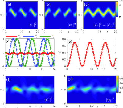
Figure 2: (Color online). (a)-(c) The evolution of the density in the two components of the soliton produced by the GP simulations for the initially balanced state with $\theta(t=0)=\pi/{4}$ and $\varphi_{-}(t=0)=\pi/4$. The parameters are $\Omega=0.5$, $\lambda=0.5\sqrt{\Omega}$, $\delta=0$, and $g=-10$. The spin dynamics and center-of-mass motion of the soliton, generated by these simulations (circles), and by the variational approximation based on Eqs. (9)-(11) and (15) (solid lines) are depicted in panels (d)-(e). Panels (f)and(g) display decay decay of the soliton in the case of weaker weaker atomic interaction, $g=-3$.

Further, in the spin representation, Eq. (5) can be written as $\dot{k}_{+}=-2\lambda\tilde{\Omega}S_{y}$, which accounts for the effect of the evolution of the spin on the center-of-mass momentum. This leads to the following equation of motion for the center-of-mass coordinate:

$$\frac{d^{2}\left\langle z\right\rangle}{dt^{2}}=-\lambda\tilde{\Omega}S_{y}\,.$$ (15)

In other words, if we consider the soliton as a macroscopic quantum body carrying the intrinsic angular momentum, Eq. (15) represents the driving force, exerted by the intrinsic momentum and acting on the linear momentum, which is literally the macroscopic SOC. We stress that the motion of the soliton differs from the collective dipole oscillations of BEC in a harmonic-potential trap under the action of the SOC, which is a wave effect. On the other hand, here we consider an effectively mechanical motion, which is produced by the interplay of the nonlinear self-trapping and SOC.

To illustrate the soliton dynamics in detail, we display, in Fig.1, numerical solutions of Eqs. (9)-(11) and (15), with initially balanced populations in the two components, which corresponds to $\theta(t=0)=\pi/4$ and $\varphi_{-}(t=0)=\pi/4$. First, in Fig. 1(a) we show that the soliton spin moves along a closed orbit on the Bloch sphere. Accordingly, perfect periodic oscillations of the spin can be identified in Fig. 1(b), and perfectly periodic linear motion of the soliton’s central coordinate is seen in Fig. 1(c).

To test these findings obtained in the variational (i.e., effectively mechanical) approximation, we numerically solved the GP system (1) with the input in the form of BB solitons, $\psi_{\uparrow}=\sqrt{\eta/2}\left(\sin\theta_{0}\right)\>\text{sech}(\eta z)e^{i(\lambda z+\varphi_{\uparrow,0})}$ and $\psi_{\downarrow}=\sqrt{\eta/2}\left(\cos\theta_{0}\right)\>\text{sech}(\eta z)e^{i(-\lambda z+\varphi_{\downarrow,0})}$. In Figs. 2 (a)-(c), the density of the soliton’s components exhibits remarkable periodic oscillations. Note that, although the initial momenta of the two components are opposite, the soliton does not split. In Fig. 2 (d)-(e), we show that the direct GP simulations agree very well with the variational (mechanical) approximation. For weaker atomic interactions, the simulations show that solitons decay under the action of SOC for $\pi\lambda/\eta>(\pi\lambda/\eta)_{c}\approx 0.4$, as shown in Fig. 2 (f)-(g). We have also explored the evolution initiated by other inputs, such as, e.g., the initially polarized one with $\theta(t=0)=\pi/{2}$ and $\varphi_{-}(t=0)=0$, and obtained a similar dynamical behavior (see the Supplementary material for details).

We stress that these results are relevant for $\lambda\leq\sqrt{\Omega}$, where the spectrum of the single-particle Hamiltonian with the SOC terms has one minimum, and the evolution of the initial BB solitons is stable. At $\lambda>\sqrt{\Omega}$, the single-particle spectrum develops two degenerate minima, and the initially prepared solitons gradually decay under the action of the SOC, as demonstrated by the GP simulations.

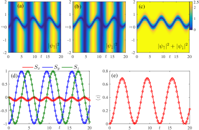
Figure 3: (Color online). (a)-(c) The same as in Fig. 2, but for the dark soliton, in the case of $g=10$.

Now, we proceed to the case of the repulsive BEC nonlinearity, which is more relevant to current experiments with SOC condensates  soc1 ; soc2 ; soc3 ; soc4 . In this case, we introduce the following variational Ansatz for dark-dark (DD) solitons:

$$\left(\begin{array}[]{c}\psi_{\uparrow}\\ \psi_{\downarrow}\end{array}\right)=\sqrt{\frac{\eta}{2}}\left(\begin{array}[]{c}\left(\sin\theta\right)\tanh(\eta z+\xi)e^{i\left(k_{\uparrow}z+\varphi_{\uparrow}\right)}\\ \left(\cos\theta\right)\tanh(\eta z+\xi)e^{i\left(k_{\downarrow}z+\varphi_{\downarrow}\right)}\end{array}\right)\,.$$ (16)

Inserting the Ansatz (16) into the Lagrangian, one needs to renormalize the integrals to exclude divergent contributions of the nonvanishing background r1 ; r2 ; r3 ; r4 ; r5 . The analysis yields the same EL equations as Eqs. (6)-(8), but with $\eta=g/2$ for repulsive $g>0$. We have also performed the respective direct simulations of the GP system with the initial conditions corresponding to the DD solitons, $\psi_{\uparrow}=\sqrt{\eta/2}\left(\sin\theta_{0}\right)\tanh(\eta z)e^{i(\lambda z+\varphi_{\uparrow,0})}$ and $\psi_{\downarrow}=\sqrt{\eta/2}\left(\cos\theta_{0}\right)\>\tanh(\eta z)e^{i(-\lambda z+\varphi_{\downarrow,0})}$. The results are depicted in Fig. 3, where the DD soliton displays oscillations similar  to those reported above for the BB configuration. Note that the two components of the background alternately disappear and revive, as shown in Fig. 3 (a)-(b).

In experiments, the condensate is usually trapped in a harmonic-oscillator potential, $V(z)=\gamma^{2}z^{2}/2$, which affect the motion of solitons d10 ; d9 ; d7 ; d11 ; HPu ; d12 . In this case, the EL equations for variational parameters $k_{+}$ and $\xi$ are modified as $\dot{k}_{+}=-2\lambda\tilde{\Omega}S_{y}+\left(\gamma^{2}/\eta\right)\xi$ and $\dot{\xi}=-{k}_{+}\eta$ with $\eta$ satisfying condition $4\eta^{4}+2g\eta^{3}=\pi^{2}\gamma^{2}$, cf. Eqs. (5) and (8). For the quasi-1D cigar-shaped BEC in our case, $\omega_{z}\ll\omega_{\bot}$, we have $\gamma\sim 0$, and the effects of trapping potential may be neglected. On the other hand, for strong trap potentials, the soliton dynamics becomes quite complex, due to the strong coupling between the spatial inhomogeneity and SOC. This issue will be considered elsewhere.

Finally, we discuss some related experimental issues. So far, the Raman-induced SOC has been realized for the BEC in the ⁸⁷Rb gas with repulsive atomic interactions. The corresponding ratios of the scattering lengths, $a_{\uparrow\uparrow}:a_{\uparrow\downarrow}:a_{\downarrow\downarrow}=1:1:1.005$ soc1 , corroborate our assumption of equal interaction strengths. In this case, the DD solitons can be created by means of the phase- and density-engineering techniques soliton3 . We consider an elongated condensate made of $\sim 10^{4}$ atoms under trapping frequencies $\omega_{\bot}=2\pi\times 2.7$ kHz and $\omega_{z}=2\pi\times 26$ Hz. The recoil momentum $k_{L}$ can be adjusted by the angle between the two incident Raman beams. For example, for the $804.1$ nm Raman lasers intersecting at angle $20^{\circ}$, the above parameters give rise to the oscillatory motion of the DD soliton with a period $\sim 10$ ms and an amplitude $\sim 1$ $\mathrm{\mu}$m.

In summary, we have shown that the interplay of the SOC (spin-orbit coupling), Raman coupling, and intrinsic nonlinearity in quasi-1D BEC may realize the mechanism of SOC in the form of mechanical motion of bright and dark solitons, considered as macroscopic quantum bodies. The soliton’s angular momentum (spin) evolves according to the Bloch equation under the action of the effective magnetic field, and induces a force affecting the motion of the soliton’s central coordinate. The results have been obtained by means of the variational analysis and numerical simulations, which demonstrate a very good agreement. These findings suggest new directions for experimental studies of the dynamics of matter-wave solitons under the action of SOC.

- (1) K. E. Strecker, G. B. Partridge, A. G. Truscott, and R. G. Hulet, New J. Phys. 5, 73 (2003).
- (2) V. A. Brazhnyi and V. V. Konotop, Mod. Phys. Lett. B 18, 627 (2004).
- (3) F. Kh. Abdullaev, A. Gammal, A. M. Kamchatnov, and L. Tomio, Int. J. Mod. Phys. B 19, 3415 (2005).
- (4) O. Morsch and M. Oberthaler, Rev. Mod. Phys. 78, 179 (2006).
- (5) B. A. Malomed, Soliton Management in Periodic Systems (Springer, Berlin, 2006).
- (6) P. G. Kevrekidis, D. J. Frantzeskakis, R. Carretero-González, Emergent Nonlinear Phenomena in Bose-Einstein Condensates (Springer, Berlin, 2008).
- (7) D. J. Frantzeskakis, J. Phys. A: Math. Theor. 43, 213001 (2010),
- (8) Y. V. Kartashov, B. A. Malomed, and L. Torner, Rev. Mod. Phys. 83, 247 (2011).
- (9) P. G. Kevrekidis and D. J. Frantzeskakis, arXiv:1512.06754.
- (10) S. Burger, K. Bongs, S. Dettmer, W. Ertmer, K. Sengstock, A. Sanpera, G. V. Shlyapnikov, and M. Lewenstein, Phys. Rev. Lett. 83, 5198 (1999).
- (11) L. Khaykovich, F. Schreck, G. Ferrari, T. Bourdel, J. Cubizolles, L. D. Carr, Y. Castin, C. Salomon, Science 296, 1290 (2002).
- (12) K. E. Strecker, G. B. Partridge, A. G. Truscott, and R. G. Hulet, Nature (London) 417, 150 (2002).
- (13) S. L. Cornish, S. T. Thompson, and C. E. Wieman, Phys. Rev. Lett. 96, 170401 (2006); A. L. Marchant, T. P. Billam, T. P. Wiles, M. M. H. Yu, S. Gardiner, and S. L. Cornish, Nature Commun. 4, 1865 (2013).
- (14) J. H. V. Nguyen, P. Dyke, D. Luo, B. A. Malomed, and R. G. Hulet, Nature Phys. 10, 918 (2014).
- (15) Y. -J. Lin, K. Jiménez-García, and I. B. Spielman, Nature (London) 471, 83 (2011).
- (16) J. -Y. Zhang, S. -C. Ji, Z. Chen, L. Zhang, Z. -D. Du, B. Yan, G. -S. Pan, B. Zhao, Y. -J. Deng, H. Zhai, S. Chen, and J. -W. Pan, Phys. Rev. Lett. 109, 115301 (2012).
- (17) P. J. Wang, Z. -Q. Yu, Z. K. Fu, J. Miao, L. H. Huang, S. J. Chai, H. Zhai, and J. Zhang, Phys. Rev. Lett. 109, 095301 (2012).
- (18) L. W. Cheuk, A. T. Sommer, Z. Hadzibabic, T. Yefsah, W. S. Bakr, and M. W. Zwierlein, Phys. Rev. Lett. 109, 095302 (2012).
- (19) C. J. Wang, C. Gao, C.-M. Jian, and H. Zhai, Phys. Rev. Lett. 105, 160403 (2010); H. Zhai, Int. J. Mod. Phys. B 26, 1230001 (2012).
- (20) T.-L. Ho and S. Z. Zhang, Phys. Rev. Lett. 107, 150403 (2011).
- (21) Z. F. Xu, R. Lü, and L. You, Phys. Rev. A 83, 053602 (2011).
- (22) Y. P. Zhang, L. Mao, and C. W. Zhang, Phys. Rev. Lett. 108, 035302 (2012).
- (23) Y. Li, L. P. Pitaevskii, and S. Stringari, Phys. Rev. Lett. 108, 225301 (2012).
- (24) J. P. Vyasanakere, S. Zhang, and V. B. Shenoy, Phys. Rev. B 84, 014512 (2011).
- (25) H. Hu, L. Jiang, X.-J. Liu, and H. Pu, Phys. Rev. Lett. 107, 195304 (2011).
- (26) M. Gong, S. Tewari, and C. W. Zhang, Phys. Rev. Lett. 107, 195303 (2011).
- (27) Z.-Q. Yu and H. Zhai, Phys. Rev. Lett. 107, 195305 (2011).
- (28) M. Gong, G. Chen, S.-T. Jia, and C. W. Zhang, Phys. Rev. Lett. 109, 105302 (2012).
- (29) C.-L. Qu, Z. Zheng, M. Gong, et al., Nature Communication 4, 2710 (2013).
- (30) W. Zhang, W. Yi, Nature Communication 4, 2711 (2013).
- (31) V. Galitski and I. B. Spielman, Nature 494 49 (2013).
- (32) N. Goldman, G. Juzeliūnas, P. Öhberg and I. B. Spielman, Rep. Prog. Phys. 77, 126401 (2014).
- (33) H. Zhai, Rep. Prog. Phys. 78, 026001 (2014).
- (34) S.-W. Su, S.-C. Gou, Q. Sun, L. Wen, W.-M. Liu, A.-C. Ji, J. Ruseckas, and G. Juzeliūnas, Phys. Rev. A 93, 053630 (2016).
- (35) Y. Xu, Y. Zhang, and B. Wu, Phys. Rev. A 87, 013614 (2013).
- (36) Y. V. Kartashov, V. V. Konotop, and F. K. Abdullaev, Phys. Rev. Lett. 111, 060402 (2013).
- (37) V. Achilleos, J. Stockhofe, P. G. Kevrekidis, D. J. Frantzeskakis and P. Schmelcher, Europhys. Lett. 103, 20002 (2013).
- (38) V. Achilleos, D. J. Frantzeskakis, P. G. Kevrekidis, and D. E. Pelinovsky, Phys. Rev. Lett. 110, 264101 (2013).
- (39) Y. K. Liu and S. J. Yang, Europhys. Lett. 108, 30004 (2014).
- (40) Y. V. Kartashov, V. V. Konotop, and D. A. Zezyulin, Phys. Rev. A 90, 063621 (2014).
- (41) S. Gautam and S. K. Adhikari, Laser Phys. Lett. 12, 045501 (2015).
- (42) S. Gautam and S. K. Adhikari, Phys. Rev. A 91, 063617 (2015).
- (43) Y. Zhang, Y. Xu, and T. Busch, Phys. Rev. A 91, 043629 (2015)
- (44) V. Achilleos, D. J. Frantzeskakis, and P. G. Kevrekidis, Phys. Rev. A 89, 033636 (2014).
- (45) S. Peotta, F. Mireles, and M. Di Ventra, Phys. Rev. A 91, 021601 (2015).
- (46) H. Sakaguchi, B. Li, and B. A. Malomed, Phys. Rev. E 89, 032920 (2014).
- (47) L. Salasnich, W. B. Cardoso, and B. A. Malomed, Phys. Rev. A 90, 033629 (2014).
- (48) H. Sakaguchi and B. A. Malomed, Phys. Rev. E 90, 062922 (2014).
- (49) V. E. Lobanov, Y. V. Kartashov, and V. V. Konotop, Phys. Rev. Lett. 112, 180403 (2014).
- (50) P. Beličev, G. Gligorić, J. Petrović, A. Maluckov, L. Hadzievski, and B. Malomed, J. Phys. B At. Mol. Opt. Phys. 48, 065301 (2015).
- (51) Y.-C. Zhang, Z.-W. Zhou, B. A. Malomed, and H. Pu, Phys. Rev. Lett. 115, 253902 (2015).
- (52) O. Fialko, J. Brand,and U. Zulicke, Phys. Rev. A 85, 051605(R) (2012).
- (53) Y. S. Kivshar, B. A. Malomed, Rev. Mod. Phys. 61, 763 (1989).
- (54) Yu. S. Kivshar and D. E. Pelinovsky, Phys. Rep. 331, 117 (2000).
- (55) Y. S. Kivshar and G. P. Agrawal, Optical Solitons: From Fibers to Photonic Crystals (Academic Press, San Diego, 2003).
- (56) B. A. Malomed, D. Mihalache, F. Wise, and L. Torner, J. Optics B: Quant. Semicl. Opt. 7, R53 (2005).
- (57) A. S. Desyatnikov, L. Torner, and Y. S. Kivshar, Progr. Opt. 47, 1 (2005).
- (58) D. Mihalache, Rom. J. Phys. 57, 352 (2012).
- (59) V. V. Konotop, J. Yang, and D. A. Zezyulin, Rev. Mod. Phys. 88, 035002 (2016).
- (60) T. Busch and J. R. Anglin, Phys. Rev. Lett. 84, 2298 (2000); T. Busch and J. R. Anglin, Phys. Rev. Lett. 87, 010401 (2001).
- (61) L. D. Carr and Y. Castin, Phys. Rev. A 66, 063602 (2002); L. Salasnich, Phys. Rev. A 70, 053617 (2004); Z. X. Liang, Z. D. Zhang, and W. M. Liu, Phys. Rev. Lett. 94, 050402 (2005).
- (62) L. Li, B. A. Malomed, D. Mihalache, and W. M. Liu, Phys. Rev. E 73 066610 (2006).
- (63) A. Weller, J. P. Ronzheimer, C. Gross, J. Esteve, and M. K. Oberthaler, D. J. Frantzeskakis, G. Theocharis and P. G. Kevrekidis, Phys. Rev. Lett. 101, 130401 (2008).
- (64) X. X. Liu, H. Pu, B. Xiong, W. M. Liu, and J. Gong, Phys. Rev. A 79, 013423 (2009).
- (65) C. Becker, S. Stellmer, P. Soltan-Panahi, S. Dörscher, M. Baumert, E.-M. Richter, J. Kronjäger, K. Bongs, and K. Sengstock, Nature Phys. 4, 496 (2008).
- (66) Z. Chen and H. Zhai, Phys. Rev. A 86, 041604 (2012).
- (67) Y. Li, G. I. Martone, and S. Stringari, Europhys. Lett. 99, 56008 (2012).
- (68) S. V. Manakov, Sov. Phys. JETP 38, 248 (1974).
- (69) B. A. Malomed, Progr. Optics 43, 71 (2002).
- (70) R. Navarro, R. Carretero-González, and P. G. Kevrekidis, Phys. Rev. A 80, 023613 (2009); L. Wen, W. M. Liu, Y. Cai, J. M. Zhang, and J. Hu, Phys. Rev. A 85, 043602 (2012).
- (71) I. S. Gradshteyn and I. M. Ryzhik, Tables of integrals, series, and products, Seventh Edition (Elsevier: Amsterdam, 2007).
- (72) I. V. Barashenkov and A. O. Harin, Phys. Rev. Lett. 72, 1575 (1994).
- (73) R. Carretero-González, D. J. Frantzeskakis, and P. G. Kevrekidis, Nonlinearity 21, 139 (2008).
- (74) D. J. Frantzeskakis, J. Phys. A Math. Theor. 43, 213001 (2010).
- (75) Y. S. Kivshar and X. Yang, Phys. Rev. E 49, 1657 (1994).
- (76) I. M. Uzunov and V. S. Gerdjikov, Phys. Rev. A 47, 1582 (1993).