A Consumer-Centric Market for Database Computation in the Cloud

Abstract

The availability of public computing resources in the cloud has revolutionized data analysis, but requesting cloud resources often involves complex decisions for consumers. Under the current pricing mechanisms, cloud service providers offer several service options and charge consumers based on the resources they use. Before they can decide which cloud resources to request, consumers have to estimate the completion time and cost of their computational tasks for different service options and possibly for different service providers. This estimation is challenging even for expert cloud users.

We propose a new market-based framework for pricing computational tasks in the cloud. Our framework introduces an agent between consumers and cloud providers. The agent takes data and computational tasks from users, estimates time and cost for evaluating the tasks, and returns to consumers contracts that specify the price and completion time. Our framework can be applied directly to existing cloud markets without altering the way cloud providers offer and price services. In addition, it simplifies cloud use for consumers by allowing them to compare contracts, rather than choose resources directly. We present design, analytical, and algorithmic contributions focusing on pricing computation contracts, analyzing their properties, and optimizing them in complex workflows. We conduct an experimental evaluation of our market framework over a real-world cloud service and demonstrate empirically that our market ensures three key properties: (a) that consumers benefit from using the market due to competitiveness among agents, (b) that agents have an incentive to price contracts fairly, and (c) that inaccuracies in estimates do not pose a significant risk to agents’ profits. Finally, we present a fine-grained pricing mechanism for complex workflows and show that it can increase agent profits by more than an order of magnitude in some cases.

1 Introduction

The availability of public computing resources in the cloud has revolutionized data analysis. Users no longer need to purchase and maintain dedicated hardware to perform large-scale computing tasks. Instead, they can execute their tasks in the cloud with the appealing opportunity to pay for just what they need. They can choose virtual machines with a wide variety of computational capabilities, they can easily form large clusters of virtual machines to parallelize their tasks, and they can use software that is already installed and configured.

Yet, taking advantage of this newly-available computing infrastructure often requires significant expertise. The common pricing mechanism of the public cloud requires that users think about low-level resources (e.g. memory, number of cores, CPU speed, IO rates) and how those resources will translate into efficiency of the user’s task. Ultimately, users with a well-defined computational task in mind care most about two key factors: the task’s completion time and its financial cost. Unfortunately, many users lack the sophistication to navigate the complex options available in the cloud and to choose a configuration that meets their preferences.

As a simple example, imagine users who need to execute a workload of relational queries using the Amazon Relational Database Service (RDS). They need to select a machine type from a list of more than 20 possible options, including “db.m3.xlarge” (4 virtual CPUs, 15GB of memory, costing $0.370 per hour) and “db.r3.xlarge” (4 virtual CPUs, 30.5GB of memory, costing $0.475 per hour). The query workload may run more quickly using db.r3.xlarge, because it has more memory, however the hourly rate of db.r3.xlarge is also more expensive, which may result in higher overall cost. Which machine type should the users choose if they are interested in the cheapest execution? Which machine type should they choose if they are interested in the cheapest execution completing within 10 minutes? Typical users do not have enough information to make this choice, as they are often not familiar with configuration parameters or cost models.

The reality of users’ choices is even more complex since they may choose one of five data management systems through RDS, or other query engines using EC2, including parallel processing engines, and different configuration options for each. They might also be tempted to compare multiple service providers, in which case they would have to deal with different pricing mechanisms in addition to different configuration options. Amazon RDS charges based on the capacity and number of computational nodes per hour; Google BigQuery charges based on the size of data processed; Microsoft Azure SQL Database charges based on the capacities of service tiers like database size limit and transaction rate.

As a result of this complexity, many users of public cloud resources make naïve, suboptimal choices that result in overpayment, and/or performance that is contrary to their preferences (e.g., it exceeds their desired deadline or exceeds their budget). Thus, instead of paying only for what they need, the reality is that they pay for what they do not need and, even worse, they pay more than they have to for it.

A market for database computations

To ease the burden on users we propose a new market-based framework for pricing computational tasks in the cloud. Our framework introduces an entity called an agent, who acts as a broker between consumers and cloud service providers. The agent accepts data and computational tasks from users, estimates the time and cost for evaluating the tasks, and returns to consumers contracts that specify the price and completion time for each task.

Our market can operate in conjunction with existing cloud markets, as it does not alter the way cloud providers offer and price services. It simplifies cloud use for consumers by allowing them to compare contracts, rather than choose resources directly. The market also allows users to extract more value from public cloud resources, achieving cheaper and faster query processing than naive configurations. At the same time, a portion of the value an agent helps extract from the cloud will be earned by the agent as profit.

Agents are conceptually distinct from cloud service providers in the sense that they have their intelligent models to estimate time and cost given consumers queries. In other words, agents take the risk of estimation, while service providers simply charge based on resource consumption, which guarantees profit. In practice, an agent could be a service provider (who provides estimation as a service in addition to cloud resources), a piece of software sold to consumers, or a separate third party who provides service across multiple providers.

Scope. Our goal in this paper is not to develop a new technical approach for estimating completion time or deriving an optimal configuration for a cloud-based computation. Prior work has considered these challenges, but, in our view, has not provided a suitable solution to the complexity of cloud provisioning. The reason is that estimation, even for relatively well-defined tasks like relational workloads, is difficult. Proposed methods require complicated profiling tasks to generate models and specialize to one type of workload (e.g., Relational database [33] or MapReduce [26]). In addition, there is inherent uncertainty in prediction, caused by multi-tenancy common in the cloud [66, 55, 17, 62, 34]. Lastly, users’ preferences are complex, involving both completion time [53] and cost [51, 82, 35, 84, 38], which have been considered as separate goals [27, 42, 44], but have not been successfully integrated.

Our market-based framework incentivizes expert agents to employ combinations of existing estimation techniques to provide this functionality as a service to non-expert consumers. Users can express preferences in terms of their utility, which includes both time and cost considerations. Uncertainty in prediction becomes a risk managed by agents, and included in the price of contracts, rather than a problem for users. Ultimately our work complements research into better cost estimation in the cloud [75, 12, 27]. In fact, our market will function more effectively as such research advances and agents can exploit new techniques for better estimation.

Our work makes several contributions:

• We define a novel market for database computations, including flexible contracts reflecting user preferences.

• We formalize the agent’s task of pricing contracts and propose an efficient algorithm for optimizing contracts.

• We perform extensive evaluation on Amazon’s public cloud, using benchmark queries and real-world scientific workflows. We show that our market is practical and effective, and satisfies key properties ensuring that both consumers and agents benefit from the market.

The paper is organized as follows. We present an overview of the market and main actors in Section 2. We formally define contracts and optimal pricing of contracts in Section 3 and 4. We extend our framework to support fine-grained pricing to further optimize contracts in Section 5. In Section 6, we introduce several alternatives. In Section 7, we present a thorough evaluation of our proposed market, and demonstrate that it guarantees several important properties. Finally, we discuss related work and extension and summarize our contributions in Sections 8, 9 and 10, respectively.

2 Computation market overview

In this section, we discuss the high-level architectural components of our computation market: three types of participants and their interactions through computation contracts. Our computation market exhibits several desirable properties, which we mention in Section 2.3.

2.1 Market participants

Our goal is to model the interactions that occur in a computation market, and design the roles and framework in a way that ensures that the market functions effectively. Our computation market involves three types of participants:

Figure 1: An overview of interactions of the main participants in the computation market: the consumer, the agent, and the cloud provider.

Cloud provider.

Cloud providers are public entities that offer computational resources as a service, on a pay-as-you-go basis. These resources are often presented as virtual machine types and providers charge fees based on the capabilities of the virtual machines and the duration of their use. Our framework does not enforce any assumptions on the types, quantity, or quality of resources that a cloud provider offers.

Consumer.

A consumer is a participant in our computational market who needs to complete a computational task over a dataset $D$. We assume the computational task is a set of queries or MapReduce jobs, denoted as $\mathbf{Q}=\{Q_{1},\allowbreak Q_{2},...,\allowbreak Q_{n}\}$. We assume that the consumer does not own the computational resources needed to complete $\mathbf{Q}$, and thus needs to use cloud resources. However, the consumer may not have the expertise to determine which cloud provider to use, which resources to lease, or how to configure them. In our framework, the consumer wishes to retrieve the task results $\mathbf{Q}(D)=\{Q_{1}(D),\allowbreak Q_{2}(D),\allowbreak...,\allowbreak Q_{n}(D)\}$ within a specified timeframe, and pay for these results directly. Therefore, the consumer’s goal is to complete the task efficiently and for low cost. Different consumers have different time and cost preferences. They will describe these preferences precisely using a utility function, as described later in Section 3.1.

Agent.

Consumers’ needs are task-centric (time and price to complete a given task), whereas cloud providers’ abilities are resource-centric (time and price for a type of resource). Due to this disparity, consumers and providers do not interact directly in our framework. Rather, a semantically separate entity, the agent, is tasked with handling the interactions between consumers and cloud providers. The agent receives a task request from a consumer and, in response, calculates a price to complete the task, providing the consumer with a formal contract. We review contracts in Section 2.2, and describe them in detail in Section 3. The agent executes accepted contracts using public cloud resources, and earns a profit whenever the contract price is greater than the actual cost of executing the task. The agent’s goals are to attract business by pricing contracts competitively and to earn a profit with each transaction. One of the main challenges for the agent is to assign accurate prices to consumer requests, which requires knowledge of cloud resources, their capabilities and costs, and expertise in tuning and query prediction.

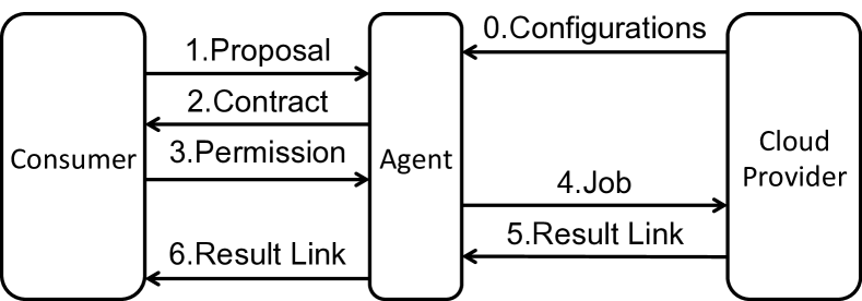
Figure 1 illustrates the interactions among the three market participants. In step 0, the agent collects details on available configurations from the cloud provider to derive later price quotes on consumers’ requests. This step may only need to be initiated once, and reused afterwards. In steps 1 through 3, the agent receives a proposal including $\mathbf{Q}$ and statistics about dataset $D$, denoted $s_{D}$, which are sufficient for pricing. For example, $s_{D}$ can be the number of input records in each table [5], histograms on key columns or sets of columns [73, 72, 74], a small sample of data [26], and other standard statistics relevant to the task. The agent reasons about possible configurations and estimates the completion time and financial cost of the queries, returning a priced contract to the consumer. If the consumer accepts the contract, in steps 4 through 6, the agent executes a job in the cloud according to the contract, computes the result, and returns a link to the consumer. The link can be, for example, an URL pointing to Amazon S3 or any other cloud storage service. Finally the agent receives payment based on the accepted contract and the actual completion time. We will see in Section 3.2 that contracts can involve complex prices that depend on the actual completion time.

2.2 Contracts

The contract is the core component of our framework, describing the terms of a computational task the agents will perform and the price they will receive upon completion of the task. The design of our market framework is intended to cope with the inevitable uncertainty of completion time. Therefore, our contracts support variable pricing based on the actual completion time when the answer is delivered.

We also formally model the time/cost preferences of the consumer using a utility function that we assume is shared with the agent. The main technical challenge for the agent is to price a contract of interest to a consumer. Pricing relies on the agent’s model of expected completion time for the task as well as the consumer’s utility. From the consumers’ side, they may receive and compare contracts from multiple agents in order to choose the one that maximizes their utility.

In this paper, we consider contracts and computational tasks that only involve analytic workloads. These analytic workloads are different from long-running services in the sense that their evaluation takes limited amount of time, even though this time can be several hours or days. Given this focus, we can assume that cloud resources do not change during the execution of task. This means, for example, that the capacity of virtual machines and their rate remain the same during the execution of a contract. We discuss relaxing these factors in Section 9.

2.3 Properties and assumptions

Our framework is designed to support three important properties: competitiveness, fairness, and resilience. Competitiveness guarantees that agents have an incentive to reduce runtime and/or cost for consumers. Fairness guarantees that agents have an incentive to present accurate estimates to consumers, and that they do not benefit by lying about expected completion times. Resilience means that an agent can profit in the marketplace even when their estimates of completion time are imprecise and possibly erroneous. We demonstrate empirically in Section 7 that our framework satisfies these crucial properties.

Our framework assumes honest participants; we defer the study of malicious consumers and agents to future work. Accepting an agent’s contract means the consumer’s data will be shared with the agent for evaluation of their task, however requesting contract prices from a set of agents reveals only the consumer’s statistics and task description.

Monopoly is not possible in this framework, and collusion among agents is unlikely. First, an agent cannot constitute a monopoly, since consumers may always choose to use a cloud service provider directly. A service provider cannot constitute a monopoly either, as any agent with a valid estimation model can enter the market. Second, collusion becomes unlikely as the number of agents in the market increases. Any agent who does not collude with others can offer a lower price and draw consumers, making any collusion unstable.

3 The consumer’s point-of-view

In this section, we describe the consumer’s interactions with the market. A transaction begins with a consumer who submits a request. This request reflects their utility, which is a precise description of their preferences. Later, given multiple priced contracts, the consumers can formally evaluate them according to the likely utility they will offer.

3.1 Consumer utility

One of our goals is to avoid simplistic definitions of contracts in which a task is carried out by a deadline for a single price. For one, many consumers have preferences far more complex than individual deadlines: they can tolerate a range of completion times, assuming they are priced appropriately. In addition, we want agents to compete to offer contracts that best meet the preferences of consumers.

A consumer’s preferences are somewhat complex because they involve tradeoffs between both completion time and price. We adopt the standard economic notion of consumer utility [64] and model it explicitly in our framework. A utility function precisely describes a consumer’s preferences by associating a utility value with every (time, price) pair. A utility function can encode, e.g., the fact that the consumer is indifferent to receiving their query answer in 10 minutes at a cost of $2.30 or 20 minutes at a cost of $1.90 (when these two cases have equal utility values) or that receiving an answer in 30 minutes at a cost of $0.75 is preferable to both of the above (when it has strictly greater utility).

Definition 3.1 (Utility)

Utility $U(t,\pi)$ is a real-valued function of time and price, which measures consumer satisfaction when a task is evaluated in time $t$ with price $\pi$.

Larger values for $U(t,\pi)$ mean greater utility and a preferred setting of $t$ and $\pi$. For a fixed completion time $t_{0}$, a consumer always prefers a lower price, so $U(t_{0},\pi)$ increases as $\pi$ decreases. Similarly, for a fixed price, $\pi_{0}$, a consumer always prefers a shorter completion time, so $U(t,\pi_{0})$ increases with decreasing $t$.

To simplify the representation of a consumer’s utility, we will restrict our attention to utility functions that are piecewise linear. That is, we assume the range of completion times $[0,\infty)$ is divided into a fixed set of intervals, and that utility on each interval is defined by a linear function of $t$ and $\pi$. This means that for each interval, the consumer has a (potentially different) rate at which she/he is willing to trade more time for lower price, and vice versa.

Definition 3.2 (Utility – piecewise)

A piece-wise utility function consists of a list of target times $\tau_{0},\dots,\tau_{n}$, where $0=\tau_{0}<\tau_{1}<\dots<\tau_{n-1}<\tau_{n}=\infty$, and linear functions $u_{1}(\pi,t),\dots,u_{n}(\pi,t)$. The utility is $u_{i}(\pi,t)$ for $t\in[\tau_{i-1},\tau_{i})$.

Such utility functions can express conventional deadlines, but also much more subtle preferences concerning the completion time and price of a computation.

Example 3.3

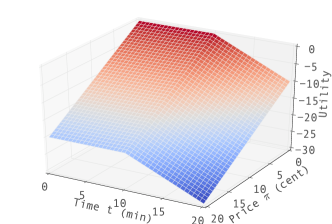
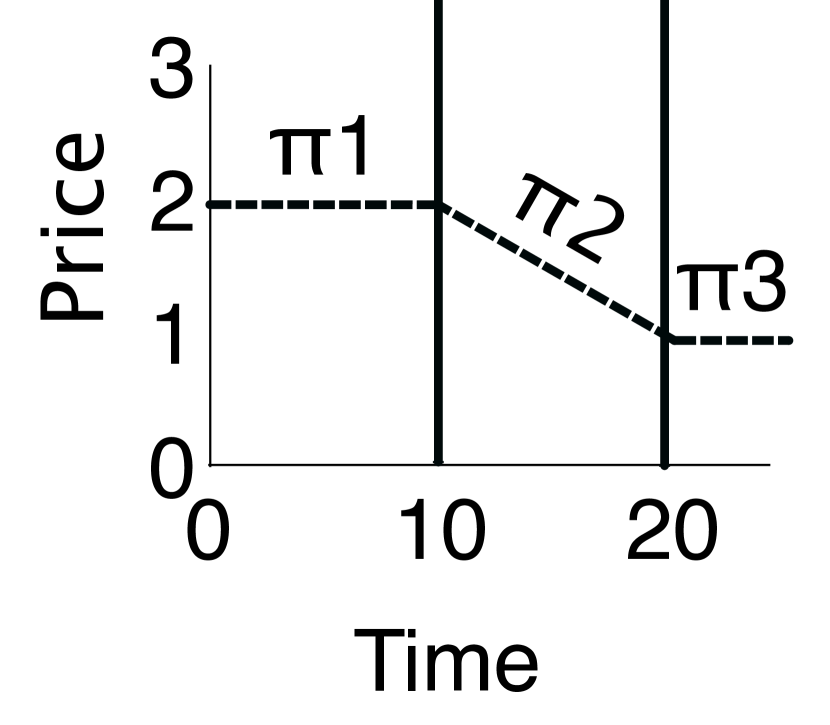
Consumer Carol has two target completion times for her computation: 10 minutes and 20 minutes. Results returned in less than 10 minutes are welcome, but she doesn’t wish to pay more to speed up the task. When results are returned between 10 minutes and 20 minutes, every minute saved is worth 1 cent to her. She does not want result returned after 20 minutes. Her piecewise utility function is:

$$U(t,\pi)=\left\{\begin{aligned} u_{1}(t,\pi)=&-\pi&(t<10)\\ u_{2}(t,\pi)=&-t-\pi+10&(10\leq t<20)\\ u_{3}(t,\pi)=&-50&(t\geq 20)\\ \end{aligned}\right.$$

Figure 2 depicts $U(t,\pi)$ when $t<20$.

In practice, users can construct the utility function by defining several critical points on a graphical user interface, or answering a few simple pair-wise preference questions.

Figure 2: Utility function for Example 3.3 when $t<20$.

3.2 Consumer contract proposal

The process of agreeing on a contract starts with the consumer advertising to agents the basic terms of a contract: the task $\mathbf{Q}$, the statistics of the database $s_{D}$, and their piecewise utility function $U$.

The terms of the contract are structured around the target times in the utility function. Agents use the utility function to choose a suitable configuration and pricing to match the preferences of the consumer. A complete, priced contract is returned to the consumer, which is defined as follows:

Definition 3.4 (Contract)

A contract is a six-tuple $\mathscr{C}=(\mathbf{Q},\allowbreak s_{D},\allowbreak\mathcal{T},\allowbreak P,\allowbreak\hat{T},\allowbreak\Pi)$, where $\mathbf{Q}$ is a task, $s_{D}$ consists of statistics about the input data, $\mathcal{T}=(\tau_{0},\tau_{1},\dots,\tau_{n})$ is an ordered list of target completion times, $P=(p_{1},\dots,p_{n})$ is an ordered list of probabilities, $\sum_{i}p_{i}=1$, $\hat{T}=(\hat{t}_{1},\dots,\hat{t}_{n})$ is an ordered list of expected completion times, and $\Pi=(\pi_{1}(t),\dots,\pi_{n}(t))$ is a list of price functions where $\pi_{i}$ is defined on $[\tau_{i-1},\tau_{i})$.

When a consumer and agent agree on a contract $\mathscr{C}$, it means that the agent has promised to deliver the answer to task $\mathbf{Q}$ on $D$ after time $t\in[0,\infty)$, where the likelihood that $t$ falls in interval $[\tau_{i-1},\tau_{i})$ is $p_{i}$. Accordingly, if the answer is delivered in the time interval $[\tau_{i-1},\tau_{i})$ the consumer agrees to pay the specified price, $\pi_{i}(t)$. $\hat{T}$ is used for computing expected utility as we will see in Section 3.3. The data statistics $s_{D}$ are given to the agent by the consumer; the agent includes them in the contract because the pricing calculation relies on these statistics.

The contract is an agreement to run the task once. The probabilities provided by the agent are a claim that if the task were run many times, a fraction of roughly $p_{i}$ of the time, the completion time would be in the interval $[\tau_{i-1},\tau_{i})$. Without this information, the consumer has no way to effectively evaluate the alternative completion times that could occur in a contract. For example, all alternatives but one could be very unlikely and this would change the meaning of the contract. We will see in Section 4 how the agent generates these probabilities.

(a)

Contracts	$\mathbf{\mathscr{C}_{1}}$	$\mathbf{\mathscr{C}_{2}}$
$\hat{T}$	$(9,15,21)$	$(9,15,21)$
$P$	$(0.2,0.5,0.3)$	$(0.1,0.8,0.1)$
Utility	-18.65	-10.4

(b)

Figure 3: (a) Price function for Example 3.5. (b) Comparison of two contracts.

Example 3.5

An example contract based on the utility function of Example 3.3 is defined by $\mathcal{T}=(0,10,20,\infty)$, probabilities $P=(0.2,0.5,0.3)$, expectations $\hat{T}=(9,15,21)$, and prices $\Pi$ (also illustrated in Figure 3(a)) defined as:

$$\Pi(t)=\left\{\begin{aligned} \pi_{1}(t)=&\>2&(t<10)\\ \pi_{2}(t)=&\>3-0.1t&(10\leq t<20)\\ \pi_{3}(t)=&\>1&(t\geq 20)\end{aligned}\right.$$

3.3 Consumer’s contract evaluation

In response to a proposed contract, a consumer hopes to receive a number of priced versions of the contract from agents. Each contract may offer the consumer a different range of utility values over the probability-weighted completion times. The consumer’s goal is to maximize their utility, so to choose between contracts, the consumer should compute the expected utility of each contract and choose the one with greatest expected utility. All contracts based on 1 utility request should share the same target completion times.

Definition 3.6 (Expected utility of a contract)

The expected utility of a contract $\mathscr{C}=(\mathbf{Q},\allowbreak s_{D},\allowbreak\mathcal{T},\allowbreak P,\allowbreak\hat{T},\allowbreak\Pi)$ with respect to utility function $U(t,\pi)$ is

$$\sum_{i=1}^{n}p_{i}u_{i}(\hat{t}_{i},\pi_{i}(\hat{t}_{i}))$$

when $u_{i}(t,\pi)$ and $\pi_{i}(t)$ are linear functions.

Example 3.7

Suppose the consumer uses the utility function in Example 3.3, and two agents return two contracts $\mathscr{C}_{1}$ and $\mathscr{C}_{2}$. Further assume both agents return the same price function $\Pi$ in Example 3.5, and the expected time $\hat{T}$ are also the same. Only the probabilities $P$ differ as illustrated in Figure 3(b). The consumer computes the expected utility according to Definition 3.6 and chooses $\mathscr{C}_{2}$ as it has greater utility.

4 The agent’s point-of-view

We now explain the agent’s interactions in the market. The agent’s main challenge is to assign prices to a contract, coping with the uncertainty of completion time, while taking into account the consumer’s utility and the market demand. We formalize two variants of pricing (risk-aware and risk-agnostic) and formulate both as optimization problems.

4.1 Pricing preliminaries

Upon receipt of the terms of a contract and the utility function of a consumer, the agent must complete the contract by computing prices for each interval and assigning probabilities to each interval.

For each configuration, we assume the financial cost $C$ borne by the agent is a function of $t$: $C(t)=\alpha_{C}\cdot t$, where $\alpha_{C}$ is the unit rate of the configuration, and can be different across configurations. Thus, the pricing of a contract depends critically on the estimate of the completion time for $\mathbf{Q}$. Since estimates of completion time are uncertain, we model completion time $T$ as a probability distribution over $[0,\infty)$ with probability density function $f_{T}(t)$. The true $f_{T}(t)$ is unlikely to be known and, in practice, must be estimated by the agent with respect to a selected configuration. Based on $f_{T}(t)$ and $C(t)$, the agent proposes a price function $\pi(t)$, which means the consumer should pay $\pi(t)$ when the completion time is $t$.

The agent has three goals when pricing a contract: (i) to maintain profitability, (ii) to offer the consumer appealing utility, and (iii) to compete with the offerings of other agents. We discuss each of these goals below.

(i) Profitability

Naturally the agents would like to price the contract higher than their cost of execution so that they can earn a profit. Profit is uncertain for an agent because it is difficult to predict completion time in the cloud. We say a contract is profitable in expectation if its expected profit, with respect to the distribution $f_{T}(t)$, is greater than zero.

$$E[\mbox{\it profit}]= \sum_{i=1}^{n}p_{i}\left(\pi_{i}(\hat{t}_{i})-C(\hat{t}_{i})\right)$$ (4.1)

We call a contract profitable (for the agent) as long as it is profitable in expectation. The agents should always price contracts so that they are profitable, but it is possible that a particular contract ends up being unprofitable.

Definition 4.1 (Profitable contract)

A profitable contract is a contract with $E[\mbox{profit}]>0$.

(ii) Prioritizing consumer utility

Since the agents knows the consumer’s utility function $U(t,\pi)$ they can (and should) take it into account when choosing a configuration and pricing. To the extent that the agents can match the consumer’s utility, their pricing of the contract will be more appealing to the consumer. The agents can evaluate the expected utility $E[U]$ over the distribution of time $T$ based on their estimates and price function $\pi(t)$:

$$E[U]=\sum_{i=1}^{n}p_{i}u_{i}(\hat{t}_{i},\pi_{i}(\hat{t}_{i}))$$ (4.2)

Profitability for the agent and utility for the consumer are conflicting objectives: a contract that offers greater profit to the agent will offer lower utility to the consumer. We will see that the agent will attempt to maximize the consumer’s utility, subject to constraints on their profitability.

(iii) Market competitiveness and demand

In all markets, including ours, market forces and competition prevent agents from raising prices without bound. In economics, a market demand function describes how these forces impact the pricing of goods [64].

When the agents decrease the price of a contract, the expected profit of the contract is reduced but they increase the utility of the contract to consumers. In a marketplace, when utility for the consumer increases, a greater number of consumers will accept the contract. Thus, the agents must balance the profit made from an individual contract with the overall profit they make from selling more contracts. To model this, we must make an assumption about the relationship between utility and the number of contracts that will be accepted by consumers in the market. This relationship is represented by the demand function which is defined as a function of utility. A linear demand curve is common in practice [64], so we focus on demand functions of the form $M(U)=a+bU$. Our framework can support demand functions of different forms, but we do not discuss these in detail.

In a real market, agents would learn about demand through repeated interactions with consumers. An agent’s demand function could depend on, for example, customer loyalty, the best contracts competitors can offer, and other factors. These factors are beyond our scope. In order to simulate the functioning of a realistic market, we must assume a demand function and, for simplicity, we assume the demand functions of all agents are the same in the rest of this paper.

4.2 Contract pricing

We start from the simplest case in which the consumer has a task $\mathbf{Q}$ and a single configuration $\phi$. So the cost function $C(t)$ and the pdf of the distribution of completion time $f_{T}(t)$ are fixed. The agent needs to define the price function $\pi(t)$ to present a competitive contract to the consumer. Let the overall profit be $\mathscr{P}$, which equals the unit profit profit multiplied by the sales $M(U)$. Notice that profit is the profit of a single contract while $\mathscr{P}$ is the overall profit of all contracts that the agent returns to all consumers in the market. The agent wants to find the price function that leads to the greatest total profit while satisfying the profitability constraint. This results in the following optimization problem:

Problem 4.2 (Contract pricing)

Given a contract $\mathscr{C}=(\mathbf{Q},\allowbreak s_{D},\allowbreak\mathcal{T},\allowbreak P,\allowbreak\hat{T},\allowbreak\Pi)$, utility function $U$, and demand function $M$, the optimal price for $\mathscr{C}$ is:

$$\mbox{maximize}: \quad\mathscr{P}=E[\mbox{profit}]\cdot E[M(U)]$$

$$\mbox{subject to}: \quad E[\mbox{profit}]>0$$

Let $I_{i}$ be the interval $(t_{i},t_{i+1})$, and recall that $p_{i}$ is the probability that the completion time falls in $I_{i}$:

$$p_{i}=\int_{t=t_{i}}^{t_{i+1}}f_{T}(t)dt$$ (4.3)

Let $T_{i}$ be a random variable of completion time in interval $I_{i}$. It is a truncated distribution with probability density function $f_{T}(t|t\in I_{i})$. Let $C_{i}$ be a random variable of cost in interval $I_{i}$. $C_{i}=C(T_{i})$. So expectation $\hat{t}_{i}$ and expectation $c_{i}$ is:

$$\hat{t}_{i}=E[T_{i}]=\int_{t\in I_{i}}tf_{T}(t|t\in I_{i})dt$$ (4.4)

$$c_{i}=E[C_{i}]=\int_{t\in I_{i}}C(t)f_{T}(t|t\in I_{i})dt$$ (4.5)

Therefore the expected unit profit and expected demand are:

$$E[\mbox{\it profit}]=\sum_{i=1}^{|I|}(\pi_{i}-c_{i})p_{i}$$ (4.6)

$$E[M(U)]=\sum_{i=1}^{|I|}M\left(U(\hat{t}_{i},\pi_{i})\right)p_{i}$$ (4.7)

Linear case

When $U$ and $M$ are linear functions, this problem becomes a convex quadratic programming problem. It has an analytical solution. More details can be found in the appendix. Here we describe the conclusion only, under the following assumptions:

• The consumer specifies a linear utility function $U(t,\pi)=-{\alpha_{U}}\cdot t-{\beta_{U}}\cdot\pi$, which means they are always willing to pay ${\alpha_{U}}$ units of cost to save ${\beta_{U}}$ units of time.

• The demand function is linear: $M(U)={\gamma_{M}}+{\lambda_{M}}\cdot U$. Thus, when $U$ increased by $1/{\lambda_{M}}$, $1$ more contract would be accepted. Since $U(t,\pi)$ is linear, the demand function can be written as $M(U)={\gamma_{M}}-{\alpha_{M}}t-{\beta_{M}}\pi$.

Applying Equations 4.6 and 4.7 to Problem 4.2, we compute the overall profit $\mathscr{P}$. $\mathscr{P}$ is maximized when

$$\mathbb{\pi}^{T}\mathbb{p}=\left\{\begin{aligned} \frac{{\gamma_{M}}-{\alpha_{M}}\mathbb{\hat{t}}^{T}\mathbb{p}+{\beta_{M}}\mathbb{c}^{T}\mathbb{p}}{2{\beta_{M}}},\;&{\gamma_{M}}-{\alpha_{M}}\mathbb{\hat{t}}^{T}\mathbb{p}-{\beta_{M}}\mathbb{c}^{T}\mathbb{p}\geq 0\\ \mathbb{c}^{T}\mathbb{p}+\epsilon,\;&otherwise\end{aligned}\right.$$

where $\epsilon$ is a small positive value, and 4 vectors $\mathbb{\pi}=[\pi_{1},\pi_{2},...]^{T}$, $\mathbb{p}=[p_{1},p_{2},...]^{T}$, $\mathbb{\hat{t}}=[\hat{t}_{1},\hat{t}_{2},...]^{T}$ and $\mathbb{c}=[c_{1},c_{2},...]^{T}$.

Furthermore, when ${\gamma_{M}}-{\alpha_{M}}\mathbb{\hat{t}}^{T}\mathbb{p}-{\beta_{M}}\mathbb{c}^{T}\mathbb{p}\geq 0$,

$$\mathscr{P}=\frac{({\gamma_{M}}-{\alpha_{M}}\mathbb{\hat{t}}^{T}\mathbb{p}-{\beta_{M}}\mathbb{c}^{T}\mathbb{p})^{2}}{4{\beta_{M}}}$$ (4.8)

Selecting a configuration

An agent typically has many available configurations for evaluating $\mathbf{Q}$. We denote the set of configurations by $\Phi=\{\phi_{1},\allowbreak\phi_{2},\allowbreak...\}$. Every configuration $\phi_{j}$ has its own cost function $C_{j}(t)=\alpha_{Cj}\cdot t$, where $\alpha_{Cj}$ is the unit rate for $\phi_{j}$.

The agent will select the configuration that results in the most profit. The distribution of time $T$ and its corresponding $p_{i}$, $\hat{t}_{i}$, and $c_{i}$ then become variables in Problem 4.2. A naïve agent can select and enumerate a small $\Phi$ to find the best possible solution. A smarter agent will use an analytic model to solve the problem [74, 27].

4.3 Risk-aware pricing

Pricing contracts involves some risk for the agents: if their estimated distributions of time and cost are different from the actual ones, they can lose profit or even suffer losses. Next, we formally define risk based on loss and add it as part of the objective.

Definition 4.3 (Loss)

Let the actual distribution of completion time be $T^{*}$ and the optimal price function be $\pi^{*}$. When the agent generates a contract with price function $\pi$, the loss of revenue $L$ is: $L_{T^{*}}(\pi)=\mathscr{P}(\pi^{*},T^{*})-\mathscr{P}(\pi,T^{*})=\mathscr{P}(\pi^{*},p^{*},t^{*},c^{*})-\mathscr{P}(\pi,p^{*},t^{*},c^{*})$, where $p^{*}$ is the actual probabilities, $t^{*}$ is the actual expected completion times, and $c^{*}$ is the actual costs.

There is always inherent uncertainty in the prediction of the distributions of completion of time and cost, so it is generally not possible for the agents to achieve the theoretically optimal profits based on the actual distributions. However, they can plan for this risk, and assess how much such risk they are willing to assume. We proceed to define risk as the worst-case possible loss that an agent can suffer.

Definition 4.4 (Risk)

The risk of the agent is a function of price $\pi$, and is defined as the maximum loss over possible distributions of completion time: $R(\pi)=\max_{T^{*}}L_{T^{*}}(\pi)$.

We incorporate risk into the agent’s optimization problem by adding it to the objective function:

$$\mbox{maximize}: \mathscr{P}(\pi,p,t,c)-\lambda R(\pi)$$ (4.9)

$$\mbox{subject to}: E[profit]>0$$

The parameter $\lambda$ in the objective is a parameter of risk that the agent is willing to assume. Larger values of $\lambda$ reduce the worst-case losses (conservative agent), while smaller values of $\lambda$ increase the assumed risk (aggressive agent). The agent can estimate the risk $R(\pi)$ by solving the following optimization problem, with variables $\pi^{*}$, $p^{*}$, $t^{*}$, and $c^{*}$:

$$\mbox{maximize}: L_{T^{*}}(\pi)=\mathscr{P}(\pi^{*},p^{*},t^{*},c^{*})-\mathscr{P}(\pi,p^{*},t^{*},c^{*})$$

$$\mbox{subject to}: E[profit^{*}]=\sum(\pi_{i}^{*}-c_{i}^{*})p_{i}^{*}>0$$

$$LBound_{t}\leq t^{*}_{i}-\hat{t}_{i}\leq UBound_{t}$$

$$LBound_{c}\leq c^{*}_{i}-c_{i}\leq UBound_{c}$$

$$0\leq p^{*}_{i}\leq 1$$

$$\sum p^{*}_{i}=1$$

where $LBound$ and $UBound$ are empirical values set by the agent. For instance, an agent’s analytic model reports estimated $\hat{t_{1}}=1$ min. However, the agent has executed 10 contracts and the actual mean of the time is $t_{1}=1.1$ min. The agent can set $LBound_{t}=0$ and $UBound_{t}=0.1$.

5 Fine-grained contract pricing

Our treatment of pricing in Section 4 assumes that agents select a single configuration for the execution of a consumer contract. However, computational tasks often contain well-separated, distinct subtasks (e.g., operators in a query plan or components in a workflow). These subtasks may have vastly different resource needs. For example, Juve et al. [32] profile multiple scientific workflow systems including Montage [30] and SIPHT [40] and find that their components have dramatically different I/O, memory and computational requirements.

We now extend our pricing framework to support fine-grained pricing, which allows agents to optimally assign separate configurations to each subtask of a computational task. It provides more candidate contracts without changing the pricing Problem 4.2. Fine-grained pricing has two benefits. First, by assigning a configuration for each subtask, instead of the entire task, agents can achieve improved time and cost, resulting in higher overall utility and/or higher profit. Second, considering subtasks separately gives agents the flexibility to outsource some computation to other agents. While outsourcing computation across agents is not a focus of our work, it is a natural fit for our fine-grained pricing mechanism. Agents can choose to outsource subtasks to other agents based on their specialization and capabilities, or for load balancing. However, some challenges of outsourcing, such as utility and forms of contracts that agents need to exchange are beyond the scope of our current work.

We model a computational task $\mathbf{Q}$ as a directed acyclic graph (DAG) $G_{\mathbf{Q}}$. Every node in $G_{\mathbf{Q}}$ is a subtask $Q_{i}$. An edge between subtasks $(Q_{i},Q_{j})$ means that the output of $Q_{i}$ is an input to $Q_{j}$. When subtasks are independent of one another, the DAG may be disconnected. Our model assumes no pipelining in subtask evaluation. Therefore, a subtask $Q_{j}$ cannot be evaluated until all subtasks $Q_{i}$, such that $(Q_{i},Q_{j})\in G_{\mathbf{Q}}$, have completed their execution.

Figure 4: An example of a simple relational query that can be broken into 3 subtasks, corresponding to different operators.

Given the graph representation $G_{\mathbf{Q}}$ of a computational task, an agent needs to determine a configuration $\phi_{i}\in\Phi$ for each subtask $Q_{i}\in\mathbf{Q}$. This is in contrast with coarse-grained pricing (Section 4.2), where the agent had to select a single configuration from $\Phi$ to be used for each subtask of $\mathbf{Q}$. When the agent chooses $\phi_{i}$, the time and cost of $Q_{i}$ is $T_{i}(\phi_{i})$ and $C_{i}(\phi_{i})$. A set of selected configurations results in total cost $C_{\mathbf{Q}}=\sum_{Q_{i}}C_{i}(\phi_{i})$, i.e., the sum of the costs of all subtasks. The completion time of $\mathbf{Q}$ is determined by the longest path ($P$) in the task graph: $T_{\mathbf{Q}}=\max_{P\in G_{\mathbf{Q}}}\sum_{Q_{i}\in P}T_{i}(\phi_{i})$. Given demand $M$ and contract utility $U$, $T_{\mathbf{Q}}$ and $C_{\mathbf{Q}}$ determine the agent’s profit $\mathscr{P}$. The goal of the agent is to select the set of configurations that maximizes $\mathscr{P}$.

Problem 5.1 (Fine-grained contract pricing)

Given graph $G_{\mathbf{Q}}$ representing a task $\mathbf{Q}$, and possible configurations $\Phi$, the agent needs to specify a configuration $\phi_{i}\in\Phi$ for each $Q_{i}\in\mathbf{Q}$, so that the time $T_{\mathbf{Q}}=\max_{P\in G_{\mathbf{Q}}}\sum_{Q_{i}\in P}T_{i}(\phi_{i})$ and cost $C_{\mathbf{Q}}=\sum_{Q_{i}}C_{i}(\phi_{i})$ maximize the overall profit $\mathscr{P}$.

Our problem definition does not model data storage and transfer time and costs explicitly. Rather, we assume that these are incorporated in the time and cost of a subtask ($T_{Q_{i}}$ and $C_{Q_{i}}$). This simplifies the model and offers an upper bound on time and cost. In practice, when two subsequent tasks share the same configuration, it is possible to reduce the costs of data passing, but these optimizations are beyond the scope of this work.

We demonstrate the intricacies of the fine-grained pricing problem through a simple example. Figure 4 shows a relational query with three distinct subtasks (operators): (1) select tuples from relation R, (2) aggregate on relation S, and (3) join of the results. We assume deterministic times and costs to evaluate each subtask, denoted next to each node in Figure 4. The select and join subtasks have only a single possible configuration each, but the aggregate subtask has two. Assume the utility function is $U(t,\pi)=-t-\pi$, which means every one minute is worth $1$ cent for the consumer. Therefore, the configuration $(2^{\prime},4\cent)$ is better for the aggregate subtask, since it has higher utility than the configuration $(5^{\prime},2\cent)$. However, following a greedy strategy that picks the configuration that is optimal for each subtask can result in sub-optimal utility for the overall task. In this example, the join subtask has to wait 5 minutes for the select subtask to complete. Therefore, there is no benefit in paying a higher price to complete the aggregate subtask sooner, making $(5^{\prime},2\cent)$ a better configuration choice.

Theorem 5.2

Fine-Grained Contract Pricing is NP-hard.

Our reduction follows from the discrete Knapsack problem (Appendix B). We next introduce a pseudo-polynomial dynamic programming algorithm for this problem, and show that it is both efficient and effective in real-world task workflows (Section 7.3). Without loss of generality, we assume that time and cost are deterministic, but the algorithm can be extended to the probabilistic case in a straightforward way.

Algorithm 1 Fine-Grained Contract Pricing

0:  $\mathbf{Q},G_{\mathbf{Q}},\Phi,\mathscr{P}(T,C)$

0:  $maximum~{}\mathscr{P}$

1:  Add node $Q_{terminal}$ with $0$ time and cost to $G_{\mathbf{Q}}$

2:  for all $Q_{i}\in\mathbf{Q}$ do

3:     Add edge $(Q_{i},Q_{terminal})$ to $G_{\mathbf{Q}}$

4:  $\mathbf{Q}_{order}\Leftarrow TopologicalSort(G_{\mathbf{Q}})$

5:  $boundT\Leftarrow$ longest time to evaluate $G_{\mathbf{Q}}$

6:  for all $Q_{i}\in\mathbf{Q}_{order}$ do

7:     $f(Q_{i},0)\Leftarrow\infty$

8:     for $t\Leftarrow 1~{}\textbf{to}{}~{}boundT$ do

9:        $f(Q_{i},t)\Leftarrow f(Q_{i},t-1)$

10:        for all $\phi\in\Phi$ do

11:           $cost_{\phi}\Leftarrow\underset{q\in pred(Q_{i})}{Combine}\left(f(q,t-T_{i}(\phi))\right)+C_{i}(\phi)$

12:           if $cost_{\phi}<f(Q_{i},t)$ then

13:              $f(Q_{i},t)\Leftarrow cost_{\phi}$

14:  return  $\max_{t}\mathscr{P}(t,f(Q_{terminal},t))$

Algorithm 1 uses dynamic programming to compute the optimal profit for task graphs. The algorithm derives the exact optimal solution for cases where $G_{\mathbf{Q}}$ is a tree (e.g., relational query operators) and computes an approximation of the optimum for task graphs that are DAGs.

In Algorithm 1, $f(Q_{i},t)$ represents the minimum cost for evaluating the subgraph terminated at subtask $Q_{i}$ when it takes at most time $t$. Then, $f(Q_{i},t)$ can be computed based on a combination of the costs of the direct predecessors of $Q_{i}$ ($pred(Q_{i})$) in the task workflow (lines 7–13). When $G_{\mathbf{Q}}$ is a tree, the $Combine$ function (line 11) is simply the sum of the costs of the predecessors ($\sum_{q\in pred(Q_{i})}f(q,t-T_{i}(\phi))$), and Algorithm 1 results in the optimal profit.

If $G_{\mathbf{Q}}$ is not a tree, predecessors of a subtask $Q_{i}$ can share common indirect predecessors, which introduces complex dependencies in the choice of configurations across different subtrees. For example, let $q_{1},q_{2}\in pred(Q_{i})$, and $q_{0}\in pred(q_{1})\cap pred(q_{2})$. Therefore, $q_{0}$ affects both subgraphs terminated at $q_{1}$ and $q_{2}$, respectively. This impacts the $Combine$ function in two ways. First, the cost of $q_{0}$ should be counted only once. Second, there may be discrepancies in the configuration choice for $q_{0}$ by the different subgraphs. There are three strategies to resolve the discrepancy: (1) use the configurations with minimum time $T$; (2) use the configurations with minimum cost $C$; (3) use the configurations with maximum $\mathscr{P}(T,C)$. The $Combine$ function applies the above strategies one by one, computes the time $T_{Q_{i}}$ and cost $C_{Q_{i}}$ of the subgraph terminated at $Q_{i}$, and updates $f(Q_{i},t)$ if $T_{Q_{i}}\leq t$ and $C_{Q_{i}}$ is better. Note that Strategy 1 guarantees a feasible solution whenever one exists.

6 Alternative Approaches

Benchmark-Based Approach

Floratou et al. [18] propose a Benchmark as a Service (BaaS) approach to help consumers select configurations. This new BaaS benchmarks user’s workload and use the optimal configuration to execute the workload repetitively. As they mention in the paper, changes such as growth of input data make BaaS complicated. So a BaaS provider need to monitor and react to these changes. In our approach, we do not make assumptions about the repetitiveness of workloads. The disadvantage is that consumers may pay more for repetitive workloads even when they are very similar. The advantage is that consumers do not need to worry about the change of the workloads.

We compare with the benchmark-based approach in Section 7.4.

VCG-Auction-Based Approach

VCG auction is a pricing mechanism. Its strategy-proof property makes it popular in many studies. We develop a VCG auction model and compare it with our approach. In this VCG model, a customer opens a bidding and agents bid on prices. Notice that this model defines consumers payment according to the utility instead of the pure price, which is different from the canonical VCG mode.

Assume agent $i$ proposes its contract with utility $Util_{i}$. The consumer takes the contract with the highest utility $Util_{i}$ but pays based on the second highest utility $U^{*}=\max_{j\neq i}(U_{j})$. The payment is a piecewise function $\Omega(t)=\omega_{k}(t)$. From agent i’s perspective, its cost function is $C_{i}(t)$, so its payoff is:

$$\text{\emph{payoff}}_{i}=\left\{\begin{aligned} E[\text{\emph{profit}}]=\sum_{k=1}^{n}p_{k}(\omega_{k}(\hat{t_{k}})-C_{i}(\hat{t_{k}}))&&\text{if}~{}U_{i}>\max_{j\neq i}(U_{j})\\ 0&&otherwise\\ \end{aligned}\right.$$

Here is the definition of $\Omega(t)$ when $U(t,\pi)=-{\alpha_{U}}t-{\beta_{U}}\pi$ is linear: Let $\Delta=U_{i}-U^{*}$. The inverse function of $U(t,\pi)$ is $\Pi(t,u)=(-{\alpha_{U}}t-u)/{\beta_{U}}$. We define $\Omega(t)=\Pi(t,u-\Delta)=\Pi(t,u)+\Delta/{\beta_{U}}$.

Example 6.1

Suppose the utility function is $U(t,\pi)=-t-2\pi~{}~{}~{}(0<t<\infty)$. So $\Pi(t,u)=(-t-u)/2$. When $\Delta=U_{i}-U^{*}=10$, $\Omega(t)=\Pi(t,u-\Delta)=(-t-(u-10))/2=(-t-u)/2+5$.

Theorem 6.2

When $U(t,\pi)$ is linear, the above $\Omega(t)$ satisfies:

1) $U_{i}>U^{*}>U^{C}_{i}\Rightarrow E[\text{\emph{profit}}]<0$;

2) $U^{C}_{i}>U^{*}>U_{i}\Rightarrow E[\text{\emph{profit}}]>0$.

The proof is in Appendix C. Given the payment function, we can show that our developed VCG auction is strategyproof.

Theorem 6.3

Every agent truthfully revealing its cost is a weakly-dominant strategy.

In other words, every rational agent will make its cost be the price in its contract. This proof is very similar to the proof for the canonical VCG auction. Please refer to Appendix C for detailed proof.

Our posted-price model and VCG auction model both exist in the real world market. We discussed in the related work section that neither of them dominates the other. They have 2 main differences in our case: 1) Posted-price model requires the agent to better understand the demand function of the market. Then an agent can set the price actively to gain more profit. In contrast, agents in VCG auction only needs to truthfully reveal their costs, then the price is passively decided based on the second best utility. 2) VCG auction requires a centralized auctioneer who ensures the consumers pay according to the second best utility. It makes a cross-platform market more difficult to form. Posted-price model does not have such requirement.

We quantitatively compare with the VCG-auction-based approach in Section 7.4.

Differentiated Bertrand

Multiple agents competing in the market is a typical differentiated Bertrand model. Specifically, Bertrand model solves the equilibrium of optimal prices based on all agents’ demand functions. But in practice, an individual agent can hardly know other agents’ demand function when pricing in the market. So our model assumes that each agent observes a demand function of its own price. Such demand function is valid given the other agents’ current prices. An agent will change its price when others change. The prices will converge to the equilibrium in the long term. Now we show the connection through an example.

In a differentiated Bertrand model, suppose there are 2 agents numbered 1 and 2. Their prices are $\mu_{1}$ and $\mu_{2}$. Agent 1’s demand function is $M_{1}(\mu_{1},\mu_{2})=\gamma-\alpha\mu_{1}+\beta\mu_{2}$ where $\alpha,\beta,\gamma$ are positive parameters. Higher $\mu_{1}$ means lower $M_{1}$ but higher $\mu_{2}$ means higher $M_{1}$ due to competition. Similarly, $M_{2}(\mu_{1},\mu_{2})=\gamma-\alpha\mu_{2}+\beta\mu_{1}$. So the overall profit $\mathscr{P}_{1}=M_{1}(\mu_{1},\mu_{2})\cdot\mu_{1}$ , $\mathscr{P}_{2}=M_{2}(\mu_{1},\mu_{2})\cdot\mu_{2}$. Given a fixed $\mu_{1}$, the best $\mu_{2}$ that maximizes $\mathscr{P}_{2}$ is:

$$\mu_{2}^{*}=(\gamma+\beta\mu_{1})/2\alpha.$$ (6.1)

Similarly, the best $\mu_{1}$ is:

$$\mu_{1}^{*}=(\gamma+\beta\mu_{2})/2\alpha.$$ (6.2)

So one can solve these two equations to get a Nash Equilibrium: $\mu_{1}^{*}=\mu_{2}^{*}=\gamma/(2\alpha-\beta)$.

In the real world, agents’ demand functions cannot be exactly the same. Thus we should use different demand functions $M_{1}(\mu_{1},\mu_{2})=\gamma_{1}-\alpha_{1}\mu_{1}+\beta_{1}\mu_{2}$ and $M_{2}(\mu_{1},\mu_{2})=\gamma_{2}-\alpha_{2}\mu_{1}+\beta_{2}\mu_{2}$. So $\mu_{1}^{*}=(2\alpha_{2}\gamma_{1}+\beta_{1}\gamma_{2})/(4\alpha_{1}\alpha_{2}-\beta_{1}\beta_{2})$ and $\mu_{2}^{*}=(2\alpha_{1}\gamma_{2}+\beta_{2}\gamma_{1})/(4\alpha_{1}\alpha_{2}-\beta_{1}\beta_{2})$.

The above calculation, however, requires that both agents know both demand functions $M_{1}$ and $M_{2}$, which may not be a realistic assumption; one may easily obtain one’s own demand function by fitting historical data, but it may not be possible to know the other party’s demand function. Without knowledge of the other party’s demand function, one generally cannot settle for the NE $(\mu_{1}^{*},\mu_{2}^{*})$ in one shot, but has to adjust one’s price dynamically according to the observed demand function. Thus we have a repeated game here, and rational agents will follow the best response functions 6.1 and 6.2. Our approach uses exactly the same response functions, where the impact of the other agent’s price is absorbed into the intercept. More precisely, in our model, Agent 1 tries to optimize $M_{1}(\mu_{1})=\gamma_{1}^{\prime}-\alpha_{1}\mu_{1}$ where $\gamma_{1}^{\prime}=\gamma_{1}+\beta_{1}\mu_{2}$, so it sets $\mu_{1}=\gamma_{1}^{\prime}/2\alpha_{1}=(\gamma_{1}+\beta_{1}\mu_{2})/2\alpha_{1}$. Similarly, Agent 2 sets $\mu_{2}=(\gamma_{2}+\beta_{2}\mu_{1})/2\alpha_{2}$. If both agents keep updating their prices in this manner, their prices will eventually converge to the NE $(\mu_{1}^{*},\mu_{2}^{*})$. Please refer to Appendix D for more detail.

7 Experimental evaluation

In this section we evaluate our market using a real-world cloud computing platform: Amazon Web Services (AWS). Our experiments collect real-world data from a variety of relational and MapReduce task workloads, and use this data to simulate the behavior of our market entities on the AWS cloud. Our results demonstrate that our market framework offers incentives to consumers, who can execute their tasks more cost-effectively, and to agents, who make profit from providing fair and competitive contracts.

We proceed to describe our experimental setup, including computational tasks, consumer parameters, and contracts.

Type	CPU (virtual)	Memory	$/hour
db.m3.Medium	1	3.75GB	$0.095
db.m3.Large	2	7.5GB	$0.195
db.m3.xLarge	4	15GB	$0.390
db.m3.2xLarge	8	30GB	$0.775
db.r3.Large	2	15GB	$0.250
db.r3.xLarge	4	30.5GB	$0.500
db.r3.2xLarge	8	61GB	$0.995
m1.Medium	1	3.75GB	$0.109
m1.Large	2	7.5GB	$0.219
m1.xLarge	4	15GB	$0.438

Figure 5: Types of Amazon machines and associated features and costs (in January 2015). The first 7 types (db.*) are RDS configurations, whereas the last 3 (m1.*) are EMR configurations. The prefixes (db and m1) are omitted from some figures for brevity.

Data and configurations

We spent 8,106 machine hours and $3,118 in obtaining the distributions of time and cost for two types of computational tasks: relational query workloads, and MapReduce jobs.

Relational query tasks: We use the queries and data of the TPC-H benchmark to evaluate relational query workloads. We use all 22 queries of the benchmark on a 5GB dataset (scale factor 5). We use the Amazon Relational Database Service (RDS) to evaluate the workloads on 7 machine configurations, each of which has 200GB of Provisioned IOPS SSD storage, and runs PostgreSQL 9.3.5. Figure 5 lists the capacity and hourly rate of each configuration.

MapReduce tasks: We evaluate MapReduce workloads using three job types (WordCount, Sort, and Join) over 5GB of randomly generated input data. We use the Amazon Elastic MapReduce service (EMR) to test our framework on these workloads. We select 3 machine configuration types. Figure 5 lists the capacities and hourly rates of these configurations. We experimented with 4 different sizes of clusters for each machine configuration: 1, 5, 10, and 20 slave nodes.

Scientific workflows: We use real-world scientific workflows that represent computational tasks with multiple subtasks, to evaluate fine-grained pricing (Section 5). We retrieved 1,454 workflows from MyExperiment [14], one of the most popular scientific workflow repositories. These workflows were developed using Taverna 2 [71], and comprise the majority of workflows in the repository. The size of workflows ranges from 1 to 154 subtasks.

Consumer models

We simulate the consumer behavior in our framework using the utility and demand functions.

Utility: In our evaluation, utility is a linear function $U(t,\pi)=-{\alpha_{U}}t-{\beta_{U}}\pi$ modeling consumer preferences. ${\alpha_{U}}$ represents the unit cost that the consumer is willing to pay to save ${\beta_{U}}$ unit time. For our experiments, we assume $U(t,\pi)=-t-\pi$, where $t$ is measured in minutes and $\pi$ is measured in cents, which means every minute is worth 1 cent to the consumer.

Demand: In our evaluation, the demand function is linear: $M(U)={\gamma_{M}}+\lambda_{M}U$, which means that when $U$ increases by $1/\lambda_{M}$, $1$ more contract would be accepted. We use $M(U)=100+50U$ for RDS, and $M(U)=100+5U$ for EMR. $\lambda_{M}$ is smaller for EMR because the times and costs for MapReduce jobs are much larger than those of relational queries.

Contracts

All our experiments involve contracts with a deadline, which means that every consumer request specifies one target completion time. We execute each task 100 times using every configuration and set the deadline of each query as the average completion time across all configurations.

7.1 Consumer incentives

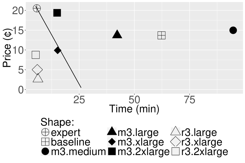
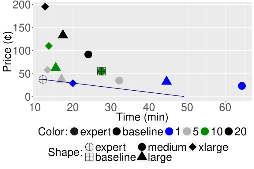
In this section, we evaluate whether our market framework offers sufficient incentive for consumers to participate in the market. Our first set of experiments simulates several naïve cloud users who select one of the default configurations for their computational tasks: 7 configurations for RDS, and 12 configurations for EMR. Then we simulate a baseline user who intuitively chooses configurations based on a simple feature of a task. Specifically, the user chooses a configuration with the best CPU performance for a CPU-intensive task, or a configuration with the best IO performance for an IO-intensive task. Predicting whether a task is CPU-intensive or IO-intensive is a difficult task for a user. However, we unfairly bias toward this baseline by indeed executing the task to measure its CPU time and IO time. We consider a task is CPU-intensive if its CPU time is greater, otherwise IO-intensive. Finally we simulate an expert agent, who, for every task, selects the configuration that maximizes the consumer’s utility function. Figure 6(a) presents the price and time achieved by each of the 7 default configurations for RDS, as well as the price and time offered by the expert agent. The line in the graph is the utility indifference curve for the agent’s configuration, representing points with the same utility value. Points on the curve are equally good, from the consumer’s perspective, as the one achieved by the expert agent. Points above the curve have worse utility values (less preferable than the agent’s offer), while points below the curve have better utility values (more preferable than the agent’s offer).

Our experiments show that the expert agent provides more utility to 4 out of 8 naïve cloud users with relational query tasks on RDS. This means that, even though the agent makes a profit, a good portion of the users would still benefit from using the market instead of relying on default settings. This effect is even more pronounced for EMR workloads. Figure 6(c) shows that the expert agent offers better utility to all simulated naïve users. This means that, in every single case, the consumers get better utility by using the agent’s services, instead of selecting a default configuration. It is noteworthy that the heuristic-based baseline approach is 189% and 67% worse in utility than our approach for RDS and EMR workloads, respectively.

(a) Utility trade-off (RDS)

(b) Agent profits and relative utilities (RDS)

(c) Utility trade-off (EMR)

(d) Agent profits and relative utilities (EMR)

Figure 6: (a, c) Users achieve better utility by using an expert agent, compared to naïvely selecting a default configuration. The agent benefits 40% of the consumers in RDS workloads, and 100% of the consumers in EMR workloads. (b, d) Expert agents always achieve the largest profits. This means that our market framework gives incentives to agents to find optimal configurations.

7.2 Agent incentives and market properties

In this section we demonstrate that the pricing framework satisfies three important properties: competitiveness, fairness, and resilience. These properties incentivize consumers and agents to use and trust the market by ensuring that (a) the agents will identify efficient computation plans and provide accurate pricing, and (b) inaccurate estimates will not pose a great risk to the agents. A theoretical analysis of the market properties is included in Appendix A.

Competitiveness

We run experiments on Amazon RDS and EMR to demonstrate how different configurations impact profitability in practice. Our goal is to show that, in our market, well-informed, expert agents can make more profit than naïve agents, thus creating incentives for agents to be competitive and offer configurations and contracts that benefit the consumers. In this experiment, a naïve agent selects one configuration to use for all queries. In contrast, the expert agent always selects the optimal configuration for each query. The goal of this experiment is to show the impact of configuration selection. Thus we control for other parameters, such as the accuracy of the agents’ estimates. So, for now, we assume that all agents know the distributions of time and cost accurately. We relax this assumption in later experiments.

	Task	Configuration
RDS	q1–q3, q5–q16, q18, q22	db.r3.Large
	q4, q17, q19, q20	db.r3.xLarge
	q21	db.r3.2xLarge
EMR	WordCount	m1.Medium $\times$ 20
	Sort	m1.Large $\times$ 5
	Join	m1.xLarge $\times$ 1

Figure 7: The expert agents select different configurations for different tasks to maximize profit.

We generate histograms of time and cost by evaluating each query with each configuration 100 times. All agents use these histograms to approximate the distributions and price contracts based on these distributions. After an agent prices a contract, we compute the number of accepted contracts according to the demand function, $M(U)$. Then we randomly select $M$ executions to do trials. The agent receives payments based on whether the execution met or missed the deadline.

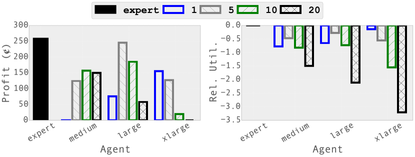
Figure 6(b) illustrates the total profit made by each agent pricing RDS workloads. There are 7 naïve agents, each using one of the RDS configurations from Figure 5, and one expert agent, who always uses the best configuration for each task. Figure 6(d) illustrates the same experiment on EMR workloads. We use one expert agent and 12 naïve agents who used the three EMR configurations from Figure 5, each with a cluster size of 1, 5, 10, or 20 nodes. Figure 7 lists the configuration chosen by the expert agent for each RDS and each EMR task. In both experiments, the expert agent achieves the highest overall profit.

Figures 6(b) and 6(d) also show the utilities offered by the agents for the same contracts. We plot the relative utility of each naïve agent, using the utility of the expert agent as a baseline: $\frac{\mathit{AgentUtility}-\mathit{ExpertUtility}}{|\mathit{ExpertUtility}|}$. On both RDS and EMR workloads, the utility offered by the expert was the best among all agents.

Our experiments on both RDS and EMR demonstrate that expert agents achieve better utility and profit than all other agents. This verifies empirically that our market design ensures incentives for agents to improve their estimation techniques and configuration selection mechanisms. This benefits both consumers, who get better utility, and agents, who get more profit.

(a) Estimate (RDS)

(b) Estimate (EMR)

(c) Fairness (RDS)

(d) Fairness (EMR)

Figure 8: Agents’ estimates are often inaccurate, and such inaccuracies can lead to loss of profit.

Fairness

Fairness guarantees the incentive for agents to present accurate estimates to consumers. If the agent uses inaccurate estimates, she/he will be penalized with lower profits. Our goal is to show that more accurate estimates lead to greater profit for the agent in practice.

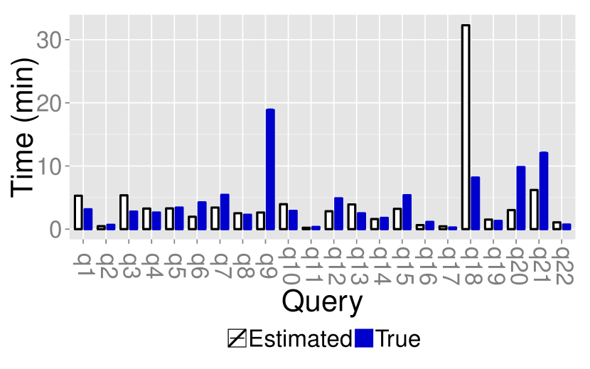
We consider an agent using db.m3.medium on RDS and PostgreSQL’s default query optimizer to estimate the completion times of queries. The PostgreSQL optimizer provides an estimate of the expected completion time and the agent assumes a Gaussian distribution with a mean value equal to the completion time predicted by the optimizer. We chose $0.05$ for the standard deviation, which is very close to the actual average standard deviation of the distributions of the 22 TPC-H queries ($0.04$).

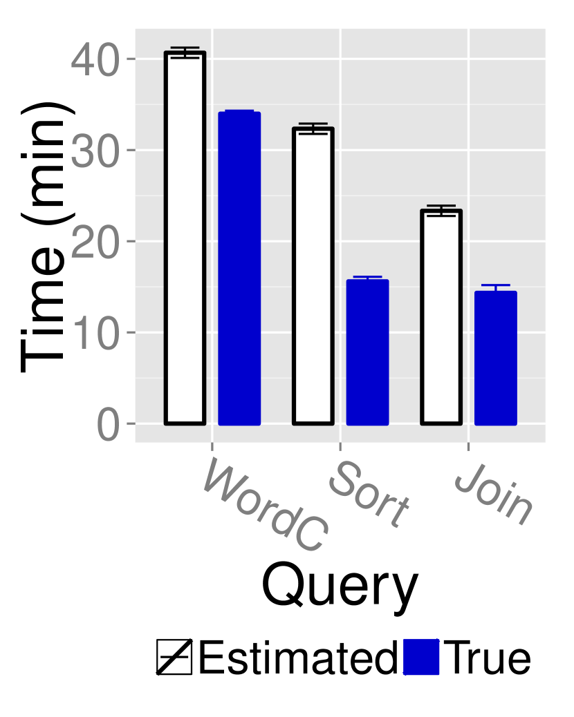
We also consider another agent using m1.medium on EMR, with one master and one slave node. The agent estimates the expected completion time by executing queries on a 5% sample of the data, and assumes a Gaussian distribution around the estimated mean. The agent uses an empirical standard deviation, $0.55$, which is close to the average true standard deviation of all three EMR job types ($0.56$).

We compare the agents’ estimate with the true distributions in Figures 8(a) and 8(b). We plot the average completion time for each TPC-H query and each EMR task. The standard deviation is very low (under 0.75 min) for all tasks. As these plots show, the agents’ estimates can often be far from the actual completion times (e.g., $q_{18}$).

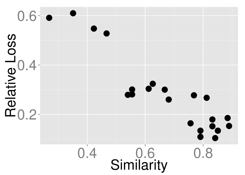
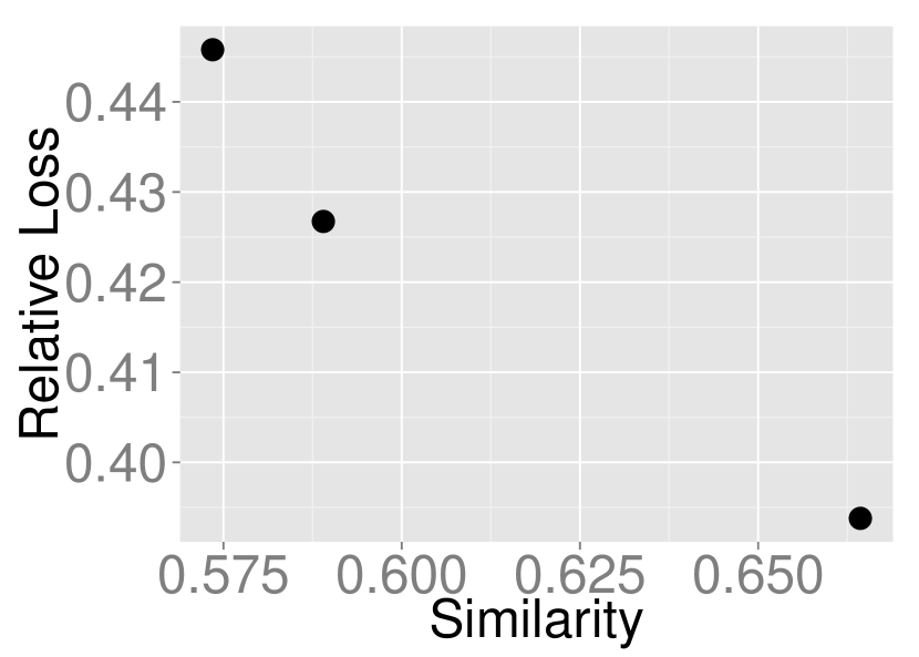
Next, we use the similarity between two distributions and relative loss to show the relationship between estimation accuracy and profit. We compare the true distribution of completion time (which is a histogram) with the agent’s estimate (a Gaussian distribution) by turning the agent’s estimate into a histogram and computing the cosine similarity between two histograms. The relative loss measures how much profit the agents lose compared to the optimal profit they could have made. We define relative loss of profit as:

$$RelativeLoss=\frac{OptimalProfit-ActualProfit}{OptimalProfit}$$ (7.1)

As Figures 8(c) and 8(d) illustrate, when the agent’s estimate is more accurate, the relative loss is smaller.

(a) (Agent’s utility - consumer’s utility) drops in overestimation.

(b) Agent’s profit decreases moderately in underestimation.

Figure 9: Poor estimation moderately impacts the market.

Our market does not rely on the assumption that the estimates are accurate, and it can in fact tolerate inaccuracies well. As long as there exists at least one task for which an agent can produce better estimates than a consumer, the agent offers utility to the market. In our experimental evaluation, we showed that this is easy to achieve in practice: even agents using simple estimation methods (such as using the PostgreSQL optimizer or sampling), which result in fairly inaccurate estimates, can provide benefit to non-expert consumers. Existing research has shown that time and cost estimation is non-trivial [1, 27, 74], and agents using such specialized tools would always produce better estimates than non-expert consumers.

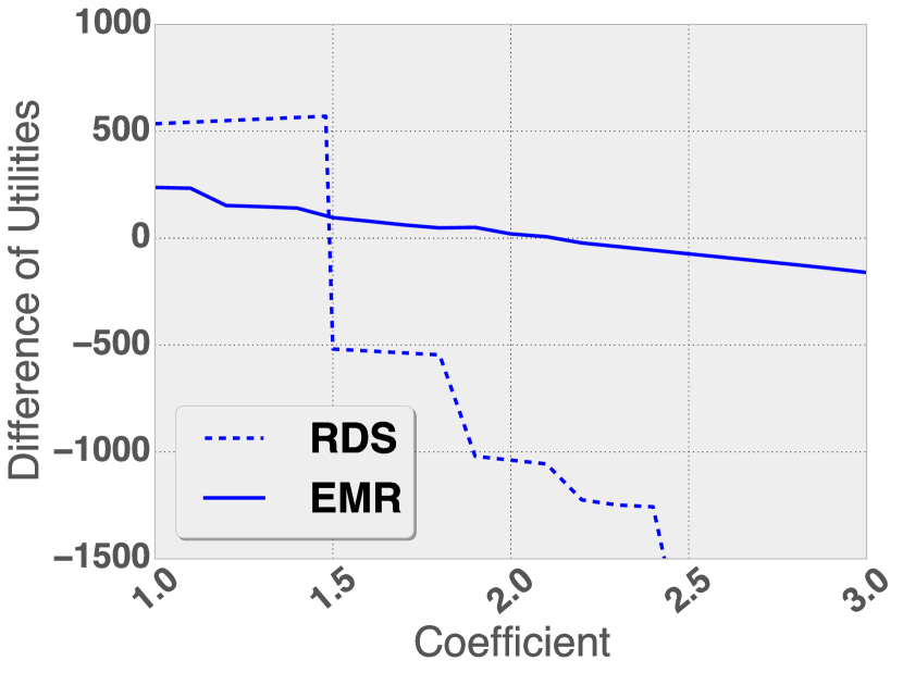
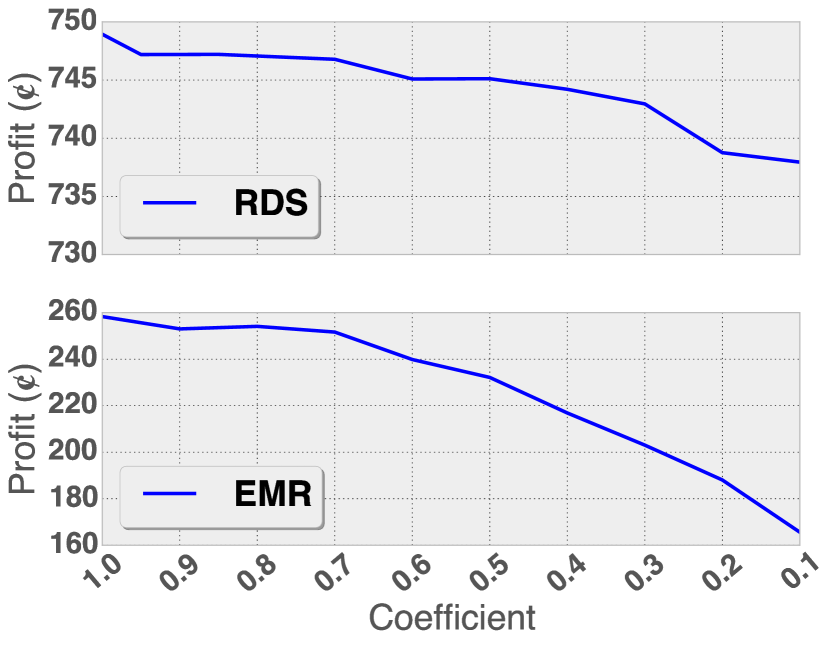
In addition, we further expanded our evaluation to study an extreme case: when all agents in the market make worse estimation than all consumers, for all tasks. We multiply the agents’ estimated time and cost by a coefficient. A $>1$ coefficient means overestimation and a $<1$ coefficient means underestimation.

As depicted in Figure 9(a), overestimation leads agents to post higher prices lowering the consumers’ utilities. However, switching to using the cloud provider directly becomes preferable (on average) only when agents overestimate substantially: in our empirical simulation, agents had to overestimate time and cost by 49% in RDS workloads, and by 120% in EMR workloads before a switch was beneficial to consumers on average.

On the other hand, figure 9(b) shows that underestimation of time and cost decreases an agent’s profit by 2% in RDS and 36% in EMR if it underestimates time and cost by a factor of 10. Depending on the agents’ profit margins, they may be able to absorb the difference without losses. To avoid losses, agents can follow risk-aware pricing strategies (Section 4.3).

(a) Resilience (RDS)

(b) Resilience (EMR)

Figure 10: By adjusting for risk, agents can reduce their losses in case of inaccurate estimates.

(a) Profit Relative to Greedy

(b) Runtime

Figure 11: DP outperforms Greedy and Search

Resilience

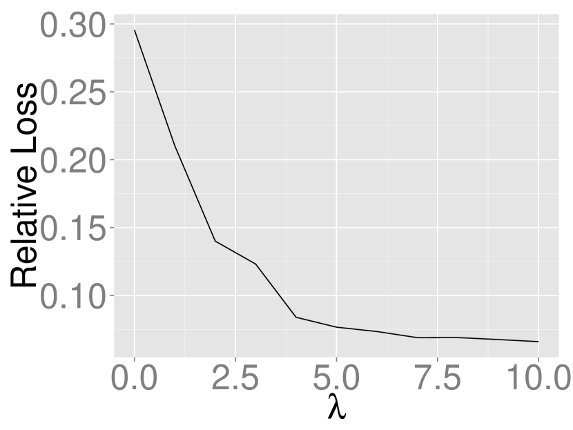
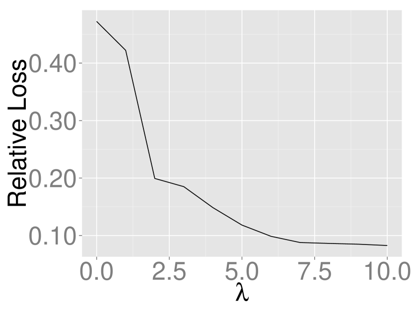
The property of resilience provides assurances to the agents, by ensuring that inaccurate estimates will not pose a significant risk to the agents’ profits. This property is crucial, as errors in the estimates are very common [5, 15, 74]. Our framework ensures resilience to these inaccuracies by accounting for risk (Definition 4.4). Specifically, the agents can profit by adjusting the risk they prefer to take. According to Equation 4.9, the risk is part of the objective and controlled by a parameter $\lambda$. When $\lambda$ is large, the agent has low confidence in the estimate (conservative). This setting reduces the loss of profit if the agent’s estimate is inaccurate.

We again consider an RDS agent using db.m3.medium and the default PostgreSQL optimizer, and an EMR agent using m1.medium and sampling to estimate runtime. We evaluate relative loss using Equation 7.1 and plot it for different values of $\lambda$ (Figure 10). A value of $\lambda=0$ means that the agent is confident that their estimate is correct. However, since in this case the estimates were inaccurate, the relative loss for $\lambda=0$ is high: the agents’ profit is much lower than the optimal profit they could have achieved. For both agents (EMR and RDS), the relative loss decreases for higher values of $\lambda$. This shows that by adjusting for risk, the agents can reduce loss of profit.

7.3 Fine-grained pricing

In our final set of experiments, we evaluate fine-grained pricing (Algorithm 1) against a large dataset of real-world scientific workflows [14]. This dataset is well-suited for this experiment, as it provides diverse computational flows of varied sizes and complexities. The published workflows do not report real execution information (time and cost), and we are not aware of any public workflow repositories that provide this information. Therefore, we augment the real workflow graphs with synthetic time and cost histograms for each subtask, drawn from random Gaussian distributions with means in the [1,100] range, and variances in the [0,5] range. Each subtask has 5 candidate configurations with different time and cost histograms. We compute the profit using utility $U(t,\pi)=-t-\pi$ and demand $M(U)=100+0.01U$ (Section 4.2). We set $\lambda_{M}$ (the coefficient of $U$) to a smaller value than the ones used for RDS and EMR workloads, because the completion times and costs for workflows are much larger.

Figure 12: Pricing at finer granularities can vastly increase the agents’ profits.

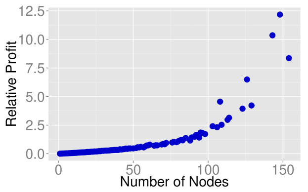
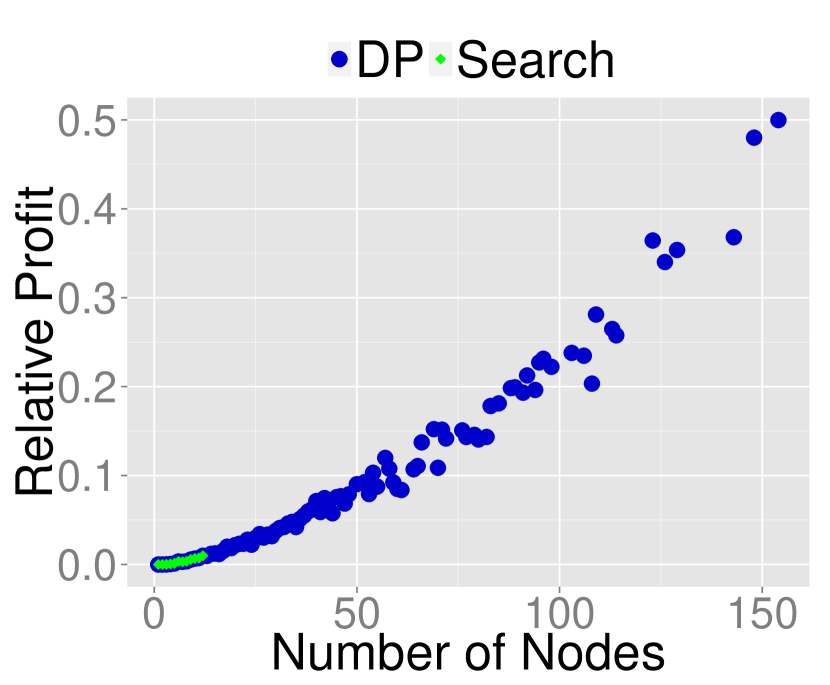
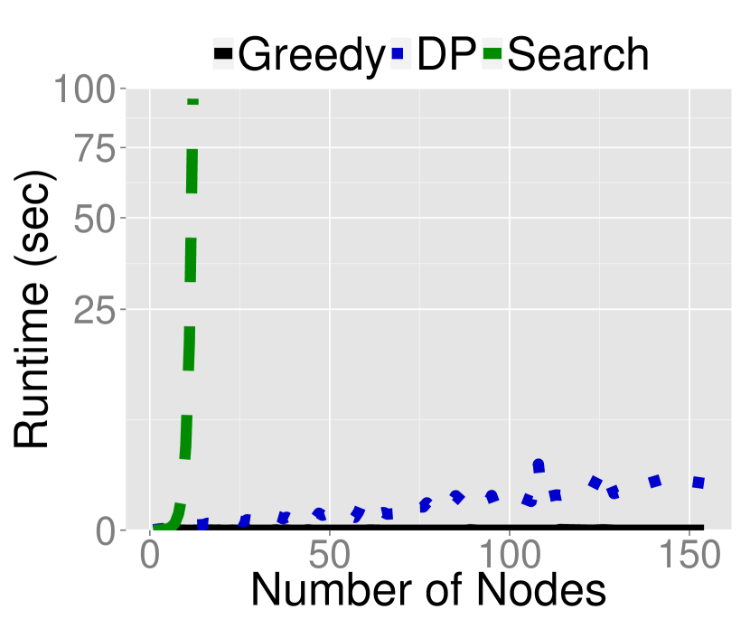
First, we evaluate our Dynamic Programming algorithm (Algorithm 1) against two baselines: (1) an exhaustive search strategy (Search) that explores all possible configuration assignments, and (2) a greedy strategy (Greedy) that selects the configuration that leads to the maximum local profit for each subtask. We perform 10 repetitions for each workflow, using different random time and cost distributions for each repetition. Figure 11(a) shows the relative profit achieved by Search and DP compared to Greedy: $\frac{\mathscr{P}-\mathscr{P}_{Greedy}}{\mathscr{P}_{Greedy}}$. DP achieves better profits than Greedy, and the effect increases for larger workflows: for workflows with 154 subtasks, DP achieves 50.0% higher profit than Greedy. Search provides few data points, as it cannot scale to larger graphs. For small workflows (up to 12 subtasks) Search and DP select equivalent configurations that result in the same (optimal) profit. Figure 11(b) shows the running time of the three algorithms. As expected, exhaustive search quickly becomes infeasible, and Greedy is faster than DP. However, the runtime of DP remains low even for larger workflows. Combined with the profit gains over Greedy, this experiment demonstrates that Algorithm 1 is highly effective for fine-grained pricing.

Second, we evaluate the benefits of fine-grained pricing, compared to coarse-grained pricing. Figure 12 shows the profit achieved by DP, which assigns a configuration to each subtask, relative to the optimal single configuration for the entire workflow. In this experiment, fine-grained pricing doubled the agents’ profits for small workflows, compared to coarse-grained pricing, and the gains increase as workflows grow larger. For the largest workflows in our dataset, fine-grained pricing achieved $12.5$ times higher profits.

7.4 Comparison with Alternative Approaches

Figure 13: Consumers prefer our approach to benchmark except for highly repetitive workloads

Benchmark-based Approach

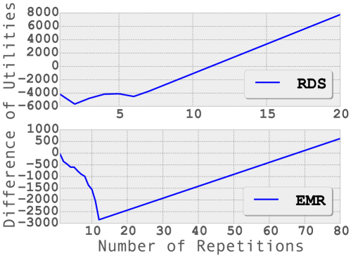
Contrasting our work with Benchmarking as a Service (BaaS) [18] is meaningful when workload repetition is significant. We assume a consumer who repeate RDS and EMR workloads without any modifications, and with each repetition tested a different configuration; once all configurations were tested, the consumer would continue using the best one in subsequent repetitions. For this experiment, we limited the number of possible configurations to 7 for RDS and 12 for EMR. This biases the experiment in favor of benchmarking, as in practice the number of configurations that the consumer would have to try is much higher. In this simplified setting, we found that it took 12 repetitions in RDS and 68 repetitions in EMR before the consumer would start benefiting from benchmarking. In the real world, these numbers are much higher, as cloud providers offer way more configurations than the ones we considered here. Cluster size alone causes an explosion in the number of options, so having an agent with an analytical model, such as in [27] , is necessary.

In practice, BaaS has additional challenges: As discussed in [18], data growth and changes in the input make BaaS complicated. Workloads are almost never repeated exactly, as the input changes between executions, requiring the BaaS provider to monitor and react to changes. Moreover, cloud providers change machine types, parameters, and pricing very frequently — e.g., between 2012 and 2015, AWS introduced on average 2.6 new instances every three months. When these settings change, resource selection needs to be re-evaluated, even if a workload stays the same.

VCG-auction-based Approach

In this experiment, we compare our model with an VCG auction model. In a strategy-proof VCG auction, the agents truthfully reveal their best costs of executing a task. Then the consumer selects the agent with the best utility but pays according to the second best utility. Therefore, given a specific task, only the best and the second best agents’ contract together define the price. So we create one agent who is always able to find the best configuration for each task, and another agent who is doing just worse than the best one. We assume a delta $\Delta$ that is the difference between the best utility and the second best utility, and vary this delta to see how much profit the best agent can get.

Figure 14: VCG auction brings less profit to agents without necessarily reducing consumers’ payments. (PP = our posted-price approach)

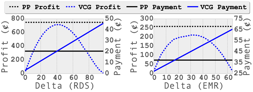
As depicted in Figure 14, when $\Delta$ becomes greater, the best agent’s profit goes up but then drops down. This is because of the demand. Larger $\Delta$ means more profit of each contract but less demand. So the profit reaches maximum at a certain point. Even this maximum VCG profit is less than the profit in our approach. It is because our approach optimizes the profit for each individual task in a workload, while the VCG approach in this experiment applies unified profit. Moreover, when $\Delta$ gets greater, consumers’ average payment for each contract is bigger. This is by definition of VCG. The VCG’s average payment goes higher than our approach’s when $\Delta$ is very small. In a word, our approach brings more profit to agents without necessarily increasing consumer’s payment.

8 Related Work

In contrast to our market framework, which emphasizes the consumer need for task-level pricing, existing work on cloud pricing largely focuses on resource usage. One study used game theory to model a pricing framework where consumers compete with each other to maximize their utilities [6, 21]. Specifically, each consumer has a demand on resources, and their utility is a function of demand and price. A choice of price by a service provider triggers a change in the consumers’ demands to maximize their utilities, thus affecting the provider’s revenue. This work makes two key assumptions that are not present in our framework. First, the chosen utility functions indicate that the quality of service (QoS) degrades when consumers share resources. While meaningful for resources such as wireless bandwidth, this assumption has been shown to not always hold in many types of resources relevant to computation [3, 4]. In fact, QoS can improve when, for example, consumers share data and cache, and agents in our framework can take advantage of this to make more profit. Second, it is assumed that the consumers know each other’s demands and strategies, and adjust their demands accordingly. In contrast, in our framework we consider consumers’ tasks separately and use probability distributions to model runtime and financial cost, leading to a simpler yet practical model.

Variants of pricing mechanisms assume that providers price dynamically, based on the consumer arrival and departure rates [7, 45, 76, 77, 78]. In turn, prices also guide consumer demand. In a different direction, Ibrahim et al. [28] argue that the interference across virtual machines sharing the same hardware leads to overcharging. They suggest cloud providers to price based on effective virtual machine time. This framework guarantees benefits to consumers and urges providers to improve their system design.

Wong et al. [31] have compared three different pricing strategies in terms of fairness and revenue: (1) Bundled pricing, in which providers sell resource bundles (e.g., virtual machine with CPU, memory, and other resources) to consumers; (2) Resource pricing, in which providers charge consumers separate prices for the consumed resources; (3) Differentiated pricing, in which providers charge consumers personalized prices. They define fairness as a function of equitability and efficiency of utilities among all consumers and conclude that differentiated pricing provides the best fairness. They treat consumers’ jobs identically and define fairness based on the number of jobs that are successfully executed by the cloud provider. They do not consider the connection between uncertain completion time and utility.

Economic-based resource allocation has been extensively studied in grid computing [10, 9, 24, 52, 34]. Researchers have developed different economic models in two main categories: “commodity markets” and “auctions”. In a commodity market, resources are sold at a posted-price. The price of resources affects consumers’ utility and demand, and therefore impacts the providers’ profit. Finding the equilibrium is the main focus in these models. Yeo et al. proposed a utility-driven pricing function [80, 56] and an autonomic pricing approach [81]. Stuer et al. [58] adapted Smale’s method [57] to price resources in grid computing markets. Bossenbroek et al. [8] introduced option contracts into the market and used hedge strategies to reduce consumers’ risk of missing task deadlines. Auction-based pricing in grid computing contains several different forms. Double auction requires consumers and providers to publish their requests and offers in a marketplace [25, 59, 69, 29]. Vickrey auction is a type of sealed-bid auction in which the highest bidder wins but pays the second-highest bid [65, 46]. Combinatorial auction allows consumers to bid on combinations of resources [13].

Posted-price selling and auctions are both established ways of selling, and it is not clear which one is better. The key challenge is the uncertainty of the value of the commodity (in this case, the computational resource) and researchers have developed different models to compare the two mechanisms under various assumptions. Computer scientists measure system metrics in these two mechanisms. Wolski et al. [70] state that posted-price brings more price stability, higher task completion rate and higher resource utilization ratio than auctions. Vanmechelen and Broeckhove [63] conclude that posted-price results in more stable pricing, while Vickrey auction results in fewer message passing in dynamic pricing. Economists have discussed the revenues in these two mechanisms. Wang [67] compares posted-price selling and auctions where the buyers have independent private values of the commodity. He finds that posted-price selling brings more profit to the seller when the buyers’ values of the commodity are widely dispersed. Campbell and Levin [11] state that auctions perform worse than posted-price when buyer valuations are interdependent. Hammond [22, 23] concludes that revenues of the two mechanisms cannot be statistically distinguished based on his study on eBay.

In contrast to our framework, this entire body of work focuses on resource-level pricing, and does not provide a mechanism for consumers to select resources based on their tasks. Recent work has started shifting the focus to task-level pricing. Floratou et al. [18] propose a Benchmark as a Service (BaaS) that benchmarks user’s workload and suggests the optimal configuration for repetitive execution. As they mention in the paper, changes such as growth of input data make BaaS complicated. In our approach, we do not assume repetitiveness of workloads. Consumers may pay more for extremely repetitive workloads, but are free from benchmarking evolved workloads.

Auction-based models [60, 61] assume that providers bid for service contracts. These models use the Vickrey-Clarke-Groves auction mechanism, which redefines the payment to the winner and guarantees that all providers report their true cost of providing the service. While this work provides a good model for task-level pricing, it does not consider execution time for tasks. In our framework, we balance the consumers’ trade-off of execution time and price through their utility function.

Personalized Service Level Agreements (PSLA) [47, 48, 49, 50] resemble the contracts in our framework, and describe a vision of a system that analyzes consumers’ data and suggests to them tiers of service. Each tier describes three properties: completion time, price per hour, querying capabilities. For example, a tier on Amazon EMR can be ($<3.5$ minutes, $0.12/hour, SELECT 1 attribute FROM 1 table WHERE condition). In our framework, consumers do not subscribe to a tier of service, but rather provide the task they need and the agent provides a specific price for the task.

When multiple agents find the same best configuration for some tasks, their prices affect each other and finally converge to the Nash Equilibrium in differentiated Bertrand model [54] in the long run.

The agents in our computation framework derive estimates of cost and time. Several approaches employ machine learning to predict the execution time of a query [19, 5]. Li et al. [37] use statistical model to estimate CPU time and other resource comsumption. Duggan et al. [15, 16] introduce special metrics and predict performance based on sampling. Wu et al. analyze the query execution plan directly to derive runtime predictions [73, 72], or use probabilistic models [74]. Ye et al. [79] perform service composition given the resource requirement of individual tasks. Uncertainty of time and cost is an important component in our framework. Existing work on scheduling SLAs considers uncertainty in the completion time when contracts specify a price. Specifically, scheduling considers 3 possible outcomes: (1) the provider accepts the SLA and returns results before the deadline, earning some profit; (2) the provider accepts the SLA but misses the deadline, and pays some penalty to the consumer; (3) the provider rejects the SLA and pays some penalty immediately. Xiong et al. [75] have developed an SLA admission control system that predicts the distribution of completion time, and accepts or rejects SLAs based on the expected profit. Chi et al. [12] assume a stream of SLAs all of which must be accepted. Their system minimizes loss by determining the execution order of SLAs based on the uncertain completion time and the penalty of missing the deadline. Liu et al. [39] have proposed an algorithm to solve tenant placement in the cloud given the distribution of completion time and the penalty of SLAs. Our market works differently in two aspects. First, our contracts consist of multiple target times, which are more flexible than the single deadline implicit in these SLAs. Second, we do not require the consumer to propose an SLA that may be rejected. Instead, the consumer makes a request that is priced by the agent according to their capabilities.

Fine-grained contract pricing is related to query optimization in distributed databases [36, 20] as we execute subtasks using different virtual machines. However, contract optimization has two objectives (time and cost), while query optimization has only one (time). These two objectives propagate differently in the task graph, making the problem more difficult.

9 Discussion

Our framework can be easily extended to handle applications with different QoS parameters. For example, in long-running services, completion time is not relevant and thus should not be part of the utility function. In contrast, other factors, such as response time, are important. These parameters are also uncertain due to unstable cloud performance [41, 68]. While we did not experiment with alternative QoS parameters and different application settings, our market framework is already equipped to handle them with appropriate changes to the utility function.

A meaningful extension to our work is to augment the market to handle varying prices. Our current framework assumes fixed prices for resource configurations. However, fluctuating prices do exist in the real world. For example, Amazon EC2 allows agents bid spot instances with much lower price [83, 2]. Agents set a maximum price threshold when requesting a spot instance. The request can be fulfilled when the market price of a spot instance is lower than this threshold. If the market price increases above the threshold, the spot instance will be terminated. In addition, agents can rent reserved instances either directly from Amazon EC2 or through its Reserved Instance Marketplace. In these cases, agents have more options to execute a task: 1) buy spot instances; 2) use their previously reserved instances; 3) buy reserved instances from others. These options introduce two additional factors to the market. First, the market needs to account for a supply function $S(\alpha_{C},t)$. This means there are $S(\alpha_{C},t)$ instances with rate $\alpha_{C}$ and available time $t$, where $\alpha_{C}$ is usually lower than the regular instance rate and $t$ must be a limited period ranging from hours to years. Second, the framework needs to consider the starting time of a task. The starting time is inconsequential when there are only regular instances with fixed rates: The agent starts regular instances whenever a consumer accepts the contract. However, the starting time matters when the rates fluctuate. In this case, agents need to estimate (a) the supply function at different points in time to ensure enough machine hours for finishing consumers’ tasks, and (b) the demand function at different points in time to decide how many instances they want to reserve. This is not a straightforward extension to our work, and will likely lead to a more complex market model.

10 Conclusions

In this paper, we propose a new marketplace framework that consumers can use to pay for well-defined database computations in the cloud. In contrast with existing pricing mechanisms, which are largely resource-centric, our framework introduces agent services that can leverage a plethora of existing tools for time, cost estimation, and scheduling, to provide consumers with personalized cloud-pricing contracts targeting a specific computational task. Agents price contracts to maximize the utility offered to consumers while also producing a profit for their services. Our market can operate in conjunction with existing cloud markets, as it does not alter the way cloud providers offer and price services. It simplifies cloud use for consumers by allowing them to compare contracts, rather than choose resources directly. The market also allows users to extract more value from public cloud resources, achieving cheaper and faster query processing than naive configurations, while a portion of this value is earned by the agents as profit for their services. Our experimental evaluation using the AWS cloud computing platform demonstrated that our market framework offers incentives to consumers, who can execute their tasks more cost-effectively, and to agents, who make profit from providing fair and competitive contracts.

Appendix A Linear case

We provide an analytical solution to the linear case, in which the utility function $U$ and demand function $M$ are linear:

• The consumers specifies a linear utility function $U(t,\pi)=-{\alpha_{U}}\cdot t-{\beta_{U}}\cdot\pi$, which means they are always willing to pay ${\alpha_{U}}$ units of cost to save ${\beta_{U}}$ units of time.

• The demand function is linear: $M(U)={\gamma_{M}}+{\lambda_{M}}\cdot U$, which means that when $U$ increased by $1/{\lambda_{M}}$, $1$ more contract would be accepted. Since $U(t,\pi)$ is linear, the demand function can be written as $M(U)={\gamma_{M}}-{\alpha_{M}}t-{\beta_{M}}\pi$.

Applying Equations 4.6 and 4.7 to Problem 4.2, we compute the overall profit as:

$$\mathscr{P}= \sum_{i=1}^{|I|}(\pi_{i}-c_{i})p_{i}\cdot\sum_{i=1}^{|I|}M\left(U(\hat{t}_{i},\pi_{i})\right)p_{i}$$

$$= (\pi-c)^{T}p\cdot\left({\gamma_{M}}-{\alpha_{M}}\hat{t}^{T}p-{\beta_{M}}\pi^{T}p\right)$$

$$= -{\beta_{M}}\left(\pi^{T}p-\frac{{\gamma_{M}}-{\alpha_{M}}\hat{t}^{T}p+{\beta_{M}}c^{T}p}{2{\beta_{M}}}\right)^{2}$$

$$+\frac{({\gamma_{M}}-{\alpha_{M}}\hat{t}^{T}p-{\beta_{M}}c^{T}p)^{2}}{4{\beta_{M}}}$$

$\mathscr{P}$ is maximized when

$$\pi^{T}p=\left\{\begin{aligned} \frac{{\gamma_{M}}-{\alpha_{M}}\hat{t}^{T}p+{\beta_{M}}c^{T}p}{2{\beta_{M}}},\;&{\gamma_{M}}-{\alpha_{M}}\hat{t}^{T}p-{\beta_{M}}c^{T}p\geq 0\\ c^{T}p+\epsilon,\;&otherwise\end{aligned}\right.$$

where $\epsilon$ is a small positive value.

Furthermore, when ${\gamma_{M}}-{\alpha_{M}}\hat{t}^{T}p-{\beta_{M}}c^{T}p\geq 0$,

$$\mathscr{P}=\frac{({\gamma_{M}}-{\alpha_{M}}\hat{t}^{T}p-{\beta_{M}}c^{T}p)^{2}}{4{\beta_{M}}}$$ (A.1)

Example A.1

Let $I={[0,\infty)}$; then $p_{1}=1$, and $\hat{t}_{1}$ is the expected completion time. The only variable is $\pi_{1}$. The problem becomes:

$$\mbox{maximize}:$$

$$\mathscr{P}= (\pi_{1}-c_{1})\cdot({\gamma_{M}}-{\alpha_{M}}\hat{t}_{1}-{\beta_{M}}\pi_{1})$$

$$\mbox{subject to}:$$

$$E[profit] =(\pi_{1}-c_{1})>0$$

The result for the price $\pi_{1}$ is:

$$\pi_{1} =max\left(\frac{{\gamma_{M}}-{\alpha_{M}}\hat{t}_{1}+{\beta_{M}}c_{1}}{2{\beta_{M}}},c_{1}+\epsilon\right)$$

We denote a configuration by its probability, time, and cost tuple: $(p,\hat{t},c)$. We can apply utility function directly to this configuration as $E[U(p,\hat{t},c)]=-{\alpha_{U}}\hat{t}^{T}p-{\beta_{U}}\pi^{T}p$. We define that a configuration $(p_{1},\hat{t}_{1},c_{1})$ is better than another configuration $(p_{2},\hat{t}_{2},c_{2})$ when $E[U(p_{1},\hat{t}_{1},c_{1})]>E[U(p_{2},\hat{t}_{2},c_{2})]$. If an agent finds a better configuration than another configuration, she/he can provide consumers greater utility (defined in Equation 4.2) while making more profit (defined in Equation 4.8). Formally:

Theorem A.2

When $E[U(p_{1},\hat{t}_{1},c_{1})]>E[U(p_{2},\hat{t}_{2},c_{2})]$, consumer’s utility $E[U_{1}]>E[U_{2}]$ and overall profit $\mathscr{P}_{1}>\mathscr{P}_{2}$.

Proof A.1.

We ignore the corner case in which ${\gamma_{M}}-{\alpha_{M}}\hat{t}^{T}p-{\beta_{M}}c^{T}p<0$, which means even the most efficient configuration found by the agent leads to zero demand. When ${\gamma_{M}}-{\alpha_{M}}\hat{t}^{T}p-{\beta_{M}}c^{T}p\geq 0$, according to Section 4.2, the overall profit $\mathscr{P}$ is maximized when $\pi^{T}p=\frac{{\gamma_{M}}-{\alpha_{M}}\hat{t}^{T}p+{\beta_{M}}c^{T}p}{2{\beta_{M}}}$. So

$$E[U]= -{\alpha_{U}}\hat{t}^{T}p-{\beta_{U}}\pi^{T}p$$

$$= -{\alpha_{U}}\hat{t}^{T}p-{\beta_{U}}\frac{{\gamma_{M}}-{\alpha_{M}}\hat{t}^{T}p+{\beta_{M}}c^{T}p}{2{\beta_{M}}}$$

$$= -{\alpha_{U}}\hat{t}^{T}p-{\beta_{U}}\frac{{\gamma_{M}}-{\lambda_{M}}{\alpha_{U}}\hat{t}^{T}p+{\lambda_{M}}{\beta_{U}}c^{T}p}{2{\lambda_{M}}{\beta_{U}}}$$

$$= -\frac{{\gamma_{M}}}{2{\lambda_{M}}}-\frac{{\alpha_{U}}\hat{t}^{T}p}{2}-\frac{{\beta_{U}}c^{T}p}{2}$$

$$= -\frac{{\gamma_{M}}}{2{\lambda_{M}}}+\frac{1}{2}E[U(p,\hat{t},c)]$$

So $E[U_{1}]>E[U_{2}]$ if $E[U(p_{1},\hat{t}_{1},c_{1})]>E[U(p_{2},\hat{t}_{2},c_{2})]$.

In addition,

$$\mathscr{P}= \frac{({\gamma_{M}}-{\alpha_{M}}\hat{t}^{T}p-{\beta_{M}}c^{T}p)^{2}}{4{\beta_{M}}}$$

$$= \frac{({\gamma_{M}}-{\lambda_{M}}{\alpha_{U}}\hat{t}^{T}p-{\lambda_{M}}{\beta_{U}}c^{T}p)^{2}}{4{\beta_{M}}}$$

$$= \frac{({\gamma_{M}}+{\lambda_{M}}E[U(p,\hat{t},c)])^{2}}{4{\beta_{M}}}$$

Since ${\gamma_{M}}-{\alpha_{M}}\hat{t}^{T}p-{\beta_{M}}c^{T}p={\gamma_{M}}+{\lambda_{M}}E[U(p,\hat{t},c)]\geq 0$, $\mathscr{P}_{1}>\mathscr{P}_{2}$ if $E[U(p_{1},\hat{t}_{1},c_{1})]>E[U(p_{2},\hat{t}_{2},c_{2})]$.

Appendix B Fine-grained pricing

Theorem 1.

Contract optimization in fine-grained pricing is NP-hard.

Proof B.1.

We prove this by reducing a 0-1 Knapsack problem to it. In a knapsack problem, there are $n$ items, each of which has a value $v_{i}$ and a weight $w_{i}$. The maximum weight of a knapsack is $W$. One wants to maximize the sum of values $V$ of selected items while the sum of their weights does not exceed $W$. We construct a contract optimization problem correspondingly. We make $n$ subtasks in a chain. Their time and cost are deterministic. The $i$th subtask has two options $(w_{i},v_{0}-v_{i})$ and $(0,v_{0})$, where $v_{0}=\max_{i}\{v_{i}\}$. Then let the overall profit be

$$\mathscr{P}(T,C)=\begin{cases}n*v_{0}-C&T\leq W\\ 0&T>W\end{cases}$$

So one can achieve value $V$ in the knapsack problem without exceeding weight limit $W$ if and only if the $\mathscr{P}=V$ in the contract optimization problem.

Appendix C VCG-auction-based approach

Recall the definition of $\Omega(t)$: When $U(t,\pi)=-{\alpha_{U}}t-{\beta_{U}}\pi$ is linear, let $\Delta=U_{i}-U^{*}$. The inverse function of $U(t,\pi)$ is $\Pi(t,u)=(-{\alpha_{U}}t-u)/{\beta_{U}}$. We define $\Omega(t)=\Pi(t,u-\Delta)=\Pi(t,u)+\Delta/{\beta_{U}}$.

Theorem 1.

When $U(t,\pi)$ is linear, the above $\Omega(t)$ satisfies:

1) $U_{i}>U^{*}>U^{C}_{i}\Rightarrow E[\text{\emph{profit}}]<0$;

2) $U^{C}_{i}>U^{*}>U_{i}\Rightarrow E[\text{\emph{profit}}]>0$.

Proof C.1.

1) $\Delta=U_{i}-U^{*}$ and $U_{i}>U^{*}>U_{i}^{C}$
$\Rightarrow\Delta<U_{i}-U_{i}^{C}=\sum_{k=1}^{n}p_{k}[U(\hat{t_{k}},\pi_{k})-U(\hat{t_{k}},c_{k})]$
$\Rightarrow\sum_{k=1}^{n}p_{k}[U(\hat{t_{k}},\pi_{k})-U(\hat{t_{k}},c_{k})]-\Delta>0$.
$0\leq p_{k}\leq 1$ and $\sum_{k=1}^{n}p_{k}=1$
$\Rightarrow\Delta=\sum_{k=1}^{n}p_{k}\Delta$.
So $\sum_{k=1}^{n}p_{k}[U(\hat{t_{k}},\pi_{k})-\Delta-U(\hat{t_{k}},c_{k})]>0$
$\Rightarrow\sum_{k=1}^{n}p_{k}(-{\beta_{U}}\pi_{k}-\Delta+{\beta_{U}}c_{k})>0$.
So $E[\text{\emph{profit}}]=\sum_{k=1}^{n}p_{k}(\omega_{k}(\hat{t_{k}})-C_{i}(\hat{t_{k}}))=-\sum_{k=1}^{n}p_{k}(-{\beta_{U}}\pi_{k}-\Delta+{\beta_{U}}c_{k})<0$.

Therefore $U_{i}>U^{*}>U^{C}_{i}\Rightarrow E[\text{\emph{profit}}]<0$;

2) Similar to above, we can prove $U^{C}_{i}>U^{*}>U_{i}\Rightarrow E[\text{\emph{profit}}]>0$.

Theorem 2.

Every agent truthfully revealing its cost is a weakly-dominant strategy.

Proof C.2.

Truthfully bidding means $U_{i}=U^{C}_{i}$.

1) The strategy of overbidding, $U_{i}>U_{i}^{C}$, is dominated by truthfully bidding.

When $U^{*}>U_{i}>U_{i}^{C}$, both strategies yield $\text{\emph{payoff}}_{i}=0$.

When $U_{i}>U_{i}^{C}>U^{*}$, both strategies yield $\text{\emph{payoff}}_{i}=E[\text{\emph{profit}}]>0$.

However, when $U_{i}>U^{*}>U_{i}^{C}$, overbidding yields $\text{\emph{payoff}}_{i}=E[\text{\emph{profit}}]<0$ (Theorem 1) while truthfully bidding yields $\text{\emph{payoff}}_{i}=0$.

So overbidding is dominated by truthfully bidding.

2) The strategy of underbidding, $U_{i}<U_{i}^{C}$, is dominated by truthfully bidding.

When $U^{*}>U^{C}_{i}>U_{i}$, both strategies yield $\text{\emph{payoff}}_{i}=0$.

When $U_{i}^{C}>U_{i}>U^{*}$, both strategies yield $\text{\emph{payoff}}_{i}=E[\text{\emph{profit}}]>0$.

However, when $U_{i}^{C}>U^{*}>U_{i}$, underbidding yields $\text{\emph{payoff}}_{i}=0$ while truthfully bidding yields $\text{\emph{payoff}}_{i}=E[\text{\emph{profit}}]>0$ (Theorem 1).

So underbidding is dominated by truthfully bidding.

So truthfully bidding is a weakly-dominant strategy.

Appendix D Bertrand Model

Recall that in the Differentiated Bertrand Model with nonidentical demand functions, the best response functions are given by

$$\mu_{1}=f_{1}(\mu_{2})=a_{1}\mu_{2}+b_{1},$$ (D.1)

$$\mu_{2}=f_{2}(\mu_{1})=a_{2}\mu_{1}+b_{2},$$ (D.2)

where

$$a_{i}=\frac{\beta_{i}}{2\alpha_{i}},\quad b_{i}=\frac{\gamma_{i}}{2\alpha_{i}},\quad\text{for }i=1,2.$$

If $a_{1}a_{2}<1$, there exists a Nash Equilibrium $(\mu_{1}^{*},\mu_{2}^{*})$, which is the unique solution to the following equations,

$$\begin{cases}\mu_{1}^{*}=f_{1}(\mu_{2}^{*}),\\ \mu_{2}^{*}=f_{2}(\mu_{1}^{*}).\end{cases}$$

Suppose that both agents keep updating their prices to the best response to the currently observed price of the other party. We show that their prices eventually converges to the NE $(\mu_{1}^{*},\mu_{2}^{*})$.

We allow for asynchronous updates. Thus at the $x$-th update, there are three possibilities,

1. Only agent 1 updates his prices, in which case

   $$(\mu_{1,x+1},\mu_{2,x+1})=F_{1}(\mu_{1,x},\mu_{2,x})=(f_{1}(\mu_{2,x}),\mu_{2,x}).$$ (D.3)

2. Only agent 2 updates his prices, in which case

   $$(\mu_{1,x+1},\mu_{2,x+1})=F_{2}(\mu_{1,x},\mu_{2,x})=(\mu_{1,x},f_{2}(\mu_{1,x})).$$ (D.4)

3. Both agents update their prices, in which case

   $$(\mu_{1,x+1},\mu_{2,x+1})=F_{3}(\mu_{1,x},\mu_{2,x})=(f_{1}(\mu_{2,x}),f_{2}(\mu_{1,x})).$$ (D.5)

Thus $(\mu_{1,x},\mu_{2,x})=G_{x}\circ G_{x-1}\circ\dots\circ G_{1}(\mu_{1,0},\mu_{2,0})$, where $\mu_{1,0}$ and $\mu_{2,0}$ are the initial prices, and $G_{i}\in\{F_{1},F_{2},F_{3}\}$ for $i=1,2,\dots,x$. We assume that both agents keep updating their prices, i.e.,

$$\lim_{x\to\infty}\sum_{i=1}^{x}\mathbf{1}\{G_{i}\neq F_{1}\}=\lim_{x\to\infty}\sum_{i=1}^{x}\mathbf{1}\{G_{i}\neq F_{2}\}=\infty.$$ (D.6)

Theorem 1.

Assume $a_{1}a_{2}<1$. If both agents keep updating their prices, i.e. (D.6) holds, then for any initial prices $\mu_{1,0}$ and $\mu_{2,0}$, we have

$$\lim_{x\to\infty}(\mu_{1,x},\mu_{2,x})=(\mu_{1}^{*},\mu_{2}^{*}).$$

Proof D.1.

For any function $f$, let $f^{(0)}=\text{id}$, the identity function, and $f^{(m)}=f^{(m-1)}\circ f$ for $m\geq 1$. Note that $F_{i}^{(2)}=F_{i}$ and $F_{3}\circ F_{i}=F_{3-i}\circ F_{i}$ for $i=1,2$. By repeated applications of these relations, we obtain

$$(\mu_{1,x},\mu_{2,x})=F_{2}^{(m_{2})}\circ H_{1}^{(m)}\circ F_{1}^{(m_{1})}\circ F_{3}^{(m_{3})}(\mu_{1,0},\mu_{2,0}),$$ (D.7)

where $H_{1}=F_{1}\circ F_{2}$, $m_{1}\in\{0,1\}$, $m_{2}\in\{0,1\}$ and $m_{1}+m_{2}+m_{3}+m=N_{x}$. Note that $N_{x}$ is the number of effective updates that can potentially change the prices. Without loss of generality, we assume that $N_{x}=x$, which amounts to discarding those updates that cannot change the price of either agent.

• Case I: $m_{1}=m_{2}=m=0$

  In this case, both agents always synchronize their updates and

  $$(\mu_{1,x},\mu_{2,x})=F_{3}^{(x)}(\mu_{1,0},\mu_{2,0})$$

  $$=\begin{cases}(g_{1}^{(\frac{x}{2})}(\mu_{1,0}),g_{2}^{(\frac{x}{2})}(\mu_{2,0})),&\text{for $x$ even},\\ (g_{1}^{(\frac{x-1}{2})}\circ f_{1}(\mu_{2,0}),g_{2}^{(\frac{x-1}{2})}\circ f_{2}(\mu_{1,0})),&\text{for $x$ odd},\end{cases}$$

  where $g_{1}=f_{1}\circ f_{2}$ and $g_{2}=f_{2}\circ f_{1}$. Note that $g_{1}(\mu_{1}^{*})=\mu_{1}^{*}$, and, for any $z$,

  $$g_{1}(z)-\mu_{1}^{*}=g_{1}(z)-g_{1}(\mu_{1}^{*})=a_{1}[f_{2}(z)-f_{2}(\mu_{1}^{*})]=a_{1}a_{2}(z-\mu_{1}^{*}).$$

  Thus for any $z$,

  $$|g_{1}^{(k)}(z)-\mu_{1}^{*}|=(a_{1}a_{2})^{k}|z-\mu_{1}^{*}|\to 0,\quad\text{as }k\to\infty.$$

  Similarly, for any $z$,

  $$|g_{2}^{(k)}(z)-\mu_{2}^{*}|=(a_{1}a_{2})^{k}|z-\mu_{2}^{*}|\to 0,\quad\text{as }k\to\infty.$$ (D.8)

  It follows that

  $$\lim_{x\to\infty}(\mu_{1,x},\mu_{2,x})=(\mu_{1}^{*},\mu_{2}^{*}).$$

• Case II: $m_{1}+m_{2}+m>0$

  In this case, the agents do not always synchronize their updates and $m\to\infty$ in (D.7). By symmetry, we assume $m_{1}=1$; the other case can be dealt with similarly. Note that

  $$H_{1}^{(m)}\circ F_{1}(\mu_{1},\mu_{2})=(f_{1}\circ g_{2}^{(\lfloor\frac{m}{2}\rfloor)}(\mu_{2}),g_{2}^{(\lceil\frac{m}{2}\rceil)}(\mu_{2})).$$

  Let $(\mu_{1},\mu_{2})=F_{3}^{(m_{3})}(\mu_{1,0},\mu_{2,0})$. By (D.8),

  $$\lim_{m\to\infty}H_{1}^{(m)}\circ F_{1}(\mu_{1},\mu_{2})=(f_{1}(\mu_{2}^{*}),\mu_{2}^{*})=(\mu_{1}^{*},\mu_{2}^{*}).$$

  It follows that

  $$\lim_{x\to\infty}(\mu_{1,n},\mu_{2,n})=\lim_{m\to\infty}F_{2}^{(m_{2})}\circ H_{1}^{(m)}\circ F_{1}(\mu_{1},\mu_{2})$$

  $$=F_{2}^{(m_{2})}(\mu_{1}^{*},\mu_{2}^{*})=(\mu_{1}^{*},\mu_{2}^{*}),$$

  where in the last step we have used the fact that $(\mu_{1}^{*},\mu_{2}^{*})$ is a fixed point of $F_{2}^{(m_{2})}$ for $m_{2}=0,1$.

References

- [1] A. Aboulnaga, Z. Wang, and Z. Y. Zhang. Packing the most onto your cloud. In CloudDB, pages 25–28, 2009.
- [2] O. Agmon Ben-Yehuda, M. Ben-Yehuda, A. Schuster, and D. Tsafrir. Deconstructing amazon ec2 spot instance pricing. TEAC, 1(3):16:1–16:20, 2013.
- [3] M. Ahmad, A. Aboulnaga, S. Babu, and K. Munagala. Interaction-aware scheduling of report-generation workloads. VLDBJ, 20(4):589–615, 2011.
- [4] M. Ahmad, S. Duan, A. Aboulnaga, and S. Babu. Predicting completion times of batch query workloads using interaction-aware models and simulation. In EDBT/ICDT, pages 449–460, 2011.
- [5] M. Akdere, U. Çetintemel, M. Riondato, E. Upfal, and S. Zdonik. Learning-based query performance modeling and prediction. In ICDE, pages 390–401, 2012.
- [6] A. Al Daoud, S. Agarwal, and T. Alpcan. Brief announcement: Cloud computing games: Pricing services of large data centers. In DISC, pages 309–310, 2009.
- [7] B. An, V. Lesser, D. Irwin, and M. Zink. Automated negotiation with decommitment for dynamic resource allocation in cloud computing. In AAMAS, pages 981–988, 2010.
- [8] A. Bossenbroek, A. Tirado-Ramos, and P. Sloot. Grid resource allocation by means of option contracts. ISJ, 3(1):49–64, 2009.
- [9] R. Buyya. Market-oriented cloud computing: Vision, hype, and reality of delivering computing as the 5th utility. In CCGRID, pages 1–1, 2009.
- [10] R. Buyya, D. Abramson, and S. Venugopal. The grid economy. IEEE, 93(3):698–714, 2005.
- [11] C. M. Campbell and D. Levin. When and why not to auction. Econ. Theory, 27(3):583–596, 2006.
- [12] Y. Chi, H. Hacígümüş, W.-P. Hsiung, and J. F. Naughton. Distribution-based query scheduling. PVLDB, 6(9):673–684, 2013.
- [13] B. Chun, P. Buonadonna, A. AuYoung, C. Ng, D. Parkes, J. Shneidman, A. Snoeren, and A. Vahdat. Mirage: A microeconomic resource allocation system for sensornet testbeds. In EmNetS, pages 19–28, 2005.
- [14] D. De Roure, C. Goble, and R. Stevens. The design and realisation of the virtual research environment for social sharing of workflows. FGCS, 25(5):561–567, 2009.
- [15] J. Duggan, Y. Chi, H. Hacigumus, S. Zhu, and U. Çetintemel. Packing light: Portable workload performance prediction for the cloud. In ICDEW, pages 258–265, 2013.
- [16] J. Duggan, O. Papaemmanouil, U. Çetintemel, and E. Upfal. Contender: A resource modeling approach for concurrent query performance prediction. In EDBT, pages 109–120, 2014.
- [17] B. Farley, A. Juels, V. Varadarajan, T. Ristenpart, K. D. Bowers, and M. M. Swift. More for your money: Exploiting performance heterogeneity in public clouds. In SOCC, pages 20:1–20:14, 2012.
- [18] A. Floratou, J. M. Patel, W. Lang, and A. Halverson. When free is not really free: What does it cost to run a database workload in the cloud? In TPCTC, pages 163–179, 2012.
- [19] A. Ganapathi, H. Kuno, U. Dayal, J. L. Wiener, A. Fox, M. Jordan, and D. Patterson. Predicting multiple metrics for queries: Better decisions enabled by machine learning. In ICDE, pages 592–603, 2009.
- [20] S. Ganguly, W. Hasan, and R. Krishnamurthy. Query optimization for parallel execution. In SIGMOD, pages 9–18, 1992.
- [21] M. Hadji, W. Louati, and D. Zeghlache. Constrained pricing for cloud resource allocation. In NCA, pages 359–365, 2011.
- [22] R. G. Hammond. Comparing revenue from auctions and posted prices. IJIO, 28(1):1–9, 2010.
- [23] R. G. Hammond. A structural model of competing sellers: Auctions and posted prices. Eur. Econ. Rev., 60(C):52–68, 2013.
- [24] A. Haque, S. M. Alhashmi, and R. Parthiban. A survey of economic models in grid computing. FGCS, 27(8):1056–1069, 2011.
- [25] M. He, H.-f. Leung, and N. R. Jennings. A fuzzy-logic based bidding strategy for autonomous agents in continuous double auctions. TKDE, 15(6):1345–1363, 2003.
- [26] H. Herodotou and S. Babu. Profiling, what-if analysis, and cost-based optimization of mapreduce programs. PVLDB, 4(11):1111–1122, 2011.
- [27] H. Herodotou, F. Dong, and S. Babu. No one (cluster) size fits all: Automatic cluster sizing for data-intensive analytics. In SOCC, pages 18:1–18:14, 2011.
- [28] S. Ibrahim, B. He, and H. Jin. Towards pay-as-you-consume cloud computing. In SCC, pages 370–377, 2011.
- [29] H. Izakian, A. Abraham, and B. T. Ladani. An auction method for resource allocation in computational grids. FGCS, 26(2):228–235, 2010.
- [30] J. C. Jacob, D. S. Katz, G. B. Berriman, J. C. Good, A. C. Laity, E. Deelman, C. Kesselman, G. Singh, M. Su, T. A. Prince, and R. Williams. Montage: a grid portal and software toolkit for science-grade astronomical image mosaicking. IJCSE, 4(2):73–87, 2009.
- [31] C. Joe-Wong and S. Sen. Mathematical frameworks for pricing in the cloud: Revenue, fairness, and resource allocations. CoRR, abs/1212.0022, 2012.
- [32] G. Juve, A. Chervenak, E. Deelman, S. Bharathi, G. Mehta, and K. Vahi. Characterizing and profiling scientific workflows. FGCS, 29(3):682–692, 2013.
- [33] Z. Karampaglis, A. Gounaris, and Y. Manolopoulos. A bi-objective cost model for database queries in a multi-cloud environment. In MEDES, 2014.
- [34] T. Kiefer, H. Schön, D. Habich, and W. Lehner. A query, a minute: Evaluating performance isolation in cloud databases. In TPCTC, pages 173–187, 2014.
- [35] P. Kokkinos, T. A. Varvarigou, A. Kretsis, P. Soumplis, and E. A. Varvarigos. Cost and utilization optimization of amazon ec2 instances. In CLOUD, pages 518–525, 2013.
- [36] R. S. G. Lanzelotte, P. Valduriez, and M. Zaït. On the effectiveness of optimization search strategies for parallel execution spaces. In VLDB, pages 493–504, 1993.
- [37] J. Li, A. C. König, V. Narasayya, and S. Chaudhuri. Robust estimation of resource consumption for sql queries using statistical techniques. PVLDB, 5(11):1555–1566, 2012.
- [38] Y. Li, E. Lo, M. L. Yiu, and W. Xu. Query optimization over cloud data market. In EDBT, pages 229–240, 2015.
- [39] Z. Liu, H. Hacigümüş, H. J. Moon, Y. Chi, and W.-P. Hsiung. Pmax: Tenant placement in multitenant databases for profit maximization. In EDBT, pages 442–453, 2013.
- [40] J. Livny, H. Teonadi, M. Livny, and M. K. Waldor. High-throughput, kingdom-wide prediction and annotation of bacterial non-coding rnas. PloS one, 3(9):e3197, 2008.
- [41] D. Lorenz and A. Orda. Qos routing in networks with uncertain parameters. TON, 6(6):768–778, 1998.
- [42] M. Malawski, G. Juve, E. Deelman, and J. Nabrzyski. Cost- and deadline-constrained provisioning for scientific workflow ensembles in iaas clouds. In SC, pages 22:1–22:11, 2012.
- [43] N. G. Mankiw. Principles of Microeconomics, 7th Edition. Cengage Learning, 7th edition, 2014.
- [44] R. Marcus and O. Papaemmanouil. Wisedb: A learning-based workload management advisor for cloud databases. Proc. VLDB Endow., 9(10):780–791, 2016.
- [45] M. Mihailescu and Y. M. Teo. Dynamic resource pricing on federated clouds. In CCGrid, pages 513–517, 2010.
- [46] N. Nisan, S. London, O. Regev, and N. Camiel. Globally distributed computation over the internet-the popcorn project. In ICDCS, pages 592–601, 1998.
- [47] J. Ortiz, V. T. de Almeida, and M. Balazinska. A vision for personalized service level agreements in the cloud. In DanaC, pages 21–25, 2013.
- [48] J. Ortiz, V. T. de Almeida, and M. Balazinska. Changing the face of database cloud services with personalized service level agreements. In CIDR, 2015.
- [49] J. Ortiz, B. Lee, and M. Balazinska. Perfenforce demonstration: Data analytics with performance guarantees. In SIGMOD, pages 2141–2144, 2016.
- [50] J. Ortiz, B. Lee, M. Balazinska, and J. L. Hellerstein. Perfenforce: A dynamic scaling engine for analytics with performance guarantees. CoRR, abs/1605.09753, 2016.
- [51] S. Pandey, A. Barker, K. Gupta, and R. Buyya. Minimizing execution costs when using globally distributed cloud services. In AINA, pages 222–229, 2010.
- [52] M. B. Qureshi, M. M. Dehnavi, N. Min-Allah, M. S. Qureshi, H. Hussain, I. Rentifis, N. Tziritas, T. Loukopoulos, S. U. Khan, C.-Z. Xu, and A. Y. Zomaya. Survey on grid resource allocation mechanisms. JGC, 12(2):399–441, 2014.
- [53] L. Ramakrishnan, J. S. Chase, D. Gannon, D. Nurmi, and R. Wolski. Deadline-sensitive workflow orchestration without explicit resource control. JPDC, 71(3):343–353, 2011.
- [54] E. Rasmusen. Games and information : an introduction to game theory. Blackwell Pub., 2007.
- [55] J. Schad, J. Dittrich, and J.-A. Quiané-Ruiz. Runtime measurements in the cloud: Observing, analyzing, and reducing variance. PVLDB, 3(1-2):460–471, 2010.
- [56] C. Shin Yeo and R. Buyya. Pricing for utility-driven resource management and allocation in clusters. IJHPCA, 21(4):405–418, 2007.
- [57] S. Smale. A convergent process of price adjustment and global newton methods. J. Math. Econ., 3(2):107–120, 1976.
- [58] G. Stuer, K. Vanmechelen, and J. Broeckhove. A commodity market algorithm for pricing substitutable grid resources. FGCS, 23(5):688–701, 2007.
- [59] Z. Tan and J. R. Gurd. Market-based grid resource allocation using a stable continuous double auction. In GRID, pages 283–290, 2007.
- [60] M. Tanaka and Y. Murakami. An efficient algorithm for strategy-proof service composition. In SCC, pages 105–112, 2013.
- [61] M. Tanaka and Y. Murakami. Strategy-proof pricing for cloud service composition. TCC, PP(99):1–1, 2014.
- [62] R. Tudoran, A. Costan, G. Antoniu, and L. Bougé. A performance evaluation of azure and nimbus clouds for scientific applications. In CloudCP, pages 4:1–4:6, 2012.
- [63] K. Vanmechelen and J. Broeckhove. A comparative analysis of single-unit vickrey auctions and commodity markets for realizing grid economies with dynamic pricing. In GECON, pages 98–111, 2007.
- [64] H. Varian. Intermediate Microeconomics: A Modern Approach. W.W. Norton & Company, 2010.
- [65] C. Waldspurger, T. Hogg, B. Huberman, J. Kephart, and W. Stornetta. Spawn: a distributed computational economy. TSE, 18(2):103–117, 1992.
- [66] H. Wang, Q. Jing, R. Chen, B. He, Z. Qian, and L. Zhou. Distributed systems meet economics: Pricing in the cloud. In HotCloud, 2010.
- [67] R. Wang. Auctions versus posted-price selling. Am. Econ. Rev., 83(4), 1993.
- [68] S. Wang, Z. Zheng, Q. Sun, H. Zou, and F. Yang. Cloud model for service selection. In INFOCOM WKSHPS, pages 666–671, 2011.
- [69] M. Wieczorek, S. Podlipnig, R. Prodan, and T. Fahringer. Applying double auctions for scheduling of workflows on the grid. In SC, pages 27:1–27:11, 2008.
- [70] R. Wolski, J. S. Plank, J. Brevik, and T. Bryan. Analyzing market-based resource allocation strategies for the computational grid. IJHPCA, 15(3):258–281, 2001.
- [71] K. Wolstencroft, R. Haines, D. Fellows, A. R. Williams, D. Withers, S. Owen, S. Soiland-Reyes, I. Dunlop, A. Nenadic, P. Fisher, J. Bhagat, K. Belhajjame, F. Bacall, A. Hardisty, A. N. de la Hidalga, M. P. B. Vargas, S. Sufi, and C. A. Goble. The taverna workflow suite: designing and executing workflows of web services on the desktop, web or in the cloud. NAR, 41(Webserver-Issue):557–561, 2013.
- [72] W. Wu, Y. Chi, H. Hacígümüş, and J. F. Naughton. Towards predicting query execution time for concurrent and dynamic database workloads. PVLDB, 6(10):925–936, 2013.
- [73] W. Wu, Y. Chi, S. Zhu, J. Tatemura, H. Hacigumus, and J. Naughton. Predicting query execution time: Are optimizer cost models really unusable? In ICDE, pages 1081–1092, 2013.
- [74] W. Wu, X. Wu, H. Hacigümüş, and J. F. Naughton. Uncertainty aware query execution time prediction. PVLDB, 7(14):1857–1868, 2014.
- [75] P. Xiong, Y. Chi, S. Zhu, J. Tatemura, C. Pu, and H. HacigümüŞ. Activesla: A profit-oriented admission control framework for database-as-a-service providers. In SOCC, pages 15:1–15:14, 2011.
- [76] H. Xu and B. Li. Maximizing revenue with dynamic cloud pricing: The infinite horizon case. In ICC, pages 2929–2933, 2012.
- [77] H. Xu and B. Li. Dynamic cloud pricing for revenue maximization. TCC, 1(2):158–171, 2013.
- [78] H. Xu and B. Li. A study of pricing for cloud resources. PER, 40(4):3–12, 2013.
- [79] Z. Ye, A. Bouguettaya, and X. Zhou. Qos-aware cloud service composition based on economic models. In ICSOC, pages 111–126, 2012.
- [80] C. S. Yeo, R. Buyya, C. S. Yeo, and R. Buyya. Pricing for utility-driven resource management and allocation in clusters. In ADCOM, pages 32–41, 2004.
- [81] C. S. Yeo, S. Venugopal, X. Chu, and R. Buyya. Autonomic metered pricing for a utility computing service. FGCS, 26(8):1368–1380, 2010.
- [82] S. Yi, A. Andrzejak, and D. Kondo. Monetary cost-aware checkpointing and migration on amazon cloud spot instances. TSC, 5(4):512–524, 2012.
- [83] S. Yi, D. Kondo, and A. Andrzejak. Reducing costs of spot instances via checkpointing in the amazon elastic compute cloud. In CLOUD, pages 236–243, 2010.
- [84] A. Zhou and B. He. Transformation-based monetary cost optimizations for workflows in the cloud. TCC, 2(1):85–98, 2014.