Beyond the Standard Model

Abstract

We cover some current topics in Beyond the Standard Model phenomenology, with an emphasis on collider (particularly Large Hadron Collider) phenomenology. We begin with a review of the Standard Model and some unresolved mysteries that it leaves. Then, we shall heuristically introduce supersymmetry, grand unified theories and extra dimensions as paradigms for expanding the Standard Model. The collider phenomenology of such models is too rich and complex to review, but we give some key examples of how the new states associated with the models might be inferred in Large Hadron Collider events. Before concluding, we finish with a brief description of a quantum field theory approximation that can be used in some cases to reduce model dependence: effective field theory.

1 Introduction

We must remember that the Standard Model of particle physics is a remarkably successful physical theory. It has been tested in literally thousands of different and diverse ways. Some of its predictions (for example the anomalous electron magnetic moment) have been verified to one part in $10^{10}$, whereas some of them (particularly the ones involving low energies and the strong interactions) have only been tested at the 10$\%$ level. However, there is to date no unambiguous direct collider measurement which rules it out. The more precise predictions are sensitive to higher loops of Standard Model particles (and in principle could be affected by loops involving beyond the Standard Model particles). Going beyond the Standard Model successfully then should not upset any of these successful predictions, and so any extension is likely to only be a small perturbation, at least at the energy scales currently being probed. Let us now turn to the fundamentals that The Standard Model is built upon.

1.1 A basic theory: quantum field theory

Microscopically we have quantum mechanics and special relativity as two fundamental theories. A consistent framework incorporating these two theories is quantum field theory (QFT). In this theory the fundamental entities are quantum fields. Their excitations correspond to the physically observable elementary particles which are the basic constituents of matter as well as the mediators of all the known interactions. Therefore, fields have a particle-like character. Particles can be classified in two general classes: bosons (spin $s=n\in\mathbb{Z}$) and fermions ($s=n+\frac{1}{2}\forall n\in\mathbb{Z}$). Bosons and fermions have very different physical behaviour. The main difference is that fermions can be shown to satisfy the Pauli “exclusion principle”, which states that two identical fermions cannot occupy the same quantum state, and therefore explaining the vast diversity of atoms.

All apparently elementary matter particles are fermions, for example the leptons (including electrons and neutrinos) and quarks (that make protons, neutrons and all other hadrons). Bosons on the other hand include the photon (particle of light and mediator of electromagnetic interaction), and the mediators of all the other interactions. They are not constrained by the Pauli principle. As we shall see, supersymmetry is a symmetry that unifies bosons and fermions despite all their differences.

1.2 Basic principle: symmetry

If QFT is the basic framework to study elementary processes, one tool to learn about these processes is the concept of symmetry.

A symmetry is a transformation that can be made to a physical system leaving the physical observables unchanged. Throughout the history of science symmetry has played a very important role in better understanding nature.

1.3 Classes of symmetries

For elementary particles, we can define two general classes of symmetries:

• Space-time symmetries: These symmetries correspond to transformations on a field theory acting explicitly on the space-time coordinates,

  $$x^{\mu}\mapsto x^{\prime\mu}\left(x^{\nu}\right)\forall\{\mu,\nu\}=\{0,1,2,3\}.$$ (1)

  Some examples are rotations, translations and, more generally, Lorentz- and Poincaré transformations defining special relativity as well as general coordinate transformations that define general relativity.

• Internal symmetries: These are symmetries that correspond to transformations of the different fields in a field theory,

  $$\Phi^{a}(x)\mapsto M^{a}\,_{b}\,\Phi^{b}(x).$$ (2)

  Roman indices $a,b$ label the corresponding fields. If $M^{a}\,_{b}$ is constant then the symmetry is a global symmetry; in case of space-time dependent $M^{a}\,_{b}(x)$ the symmetry is called a local symmetry or a gauge symmetry.

1.4 Importance of symmetries

Symmetry is important for various reasons:

• Labelling and classifying particles: Symmetries label and classify particles according to the different conserved quantum numbers identified by the space-time and internal symmetries (mass, spin, charge, colour, etc.). In this regard symmetries actually “define” an elementary particle according to the behaviour of the corresponding field with respect to the different symmetries.

• Symmetries determine the interactions among particles, by means of the gauge principle, for instance. It is important that most QFTs of vector bosons are sick: they are non-renormalisable in a way that makes them lose predictivity. The counter example to this is gauge theory, where vector bosons are necessarily in the adjoint representation of the gauge group. As an illustration, consider the Lagrangian

  $${{\cal L}=\partial_{\mu}\phi\,\partial^{\mu}\phi^{*}-V(\phi,\phi^{*})}$$ (3)

  which is invariant under rotations in the complex plane

  $${\phi\mapsto\exp(i\alpha)\,\phi},$$ (4)

  as long as $\alpha$ is a constant (this corresponds to a global symmetry). If $\alpha=\alpha(x)$, the kinetic term is no longer invariant:

  $${\partial_{\mu}\phi\mapsto\exp(i\alpha)\,\bigl{(}\partial_{\mu}\phi\,+\,i(\partial_{\mu}\alpha)\phi\bigr{)}\,.}$$ (5)

  However, the covariant derivative $D_{\mu}$, defined as

  $${D_{\mu}\phi=\partial_{\mu}\phi+iA_{\mu}\,\phi,}$$ (6)

  transforms like $\phi$ itself, if the gauge - potential $A_{\mu}$ transforms to $A_{\mu}-\partial_{\mu}\alpha$:

  $${D_{\mu}\phi} \mapsto {\exp(i\alpha)\,\bigl{(}\partial_{\mu}\phi\,+\,i(\partial_{\mu}\alpha)\phi+i(A_{\mu}-\partial_{\mu}\alpha)\,\phi\bigr{)}}$$

  $$= {\exp(i\alpha)\,D_{\mu}\phi,}$$

  so we rewrite the Lagrangian to ensure gauge invariance:

  $${{\cal L}=D_{\mu}\phi\,(D^{\mu}\phi)^{*}-V(\phi,\phi^{*})\,.}$$ (7)

  The scalar field $\phi$ couples to the gauge field $A_{\mu}$ via $A_{\mu}\phi A^{\mu}\phi$, similarly, the Dirac Lagrangian

  $${{\cal L}=\overline{\Psi}\,\gamma^{\mu}\,D_{\mu}\Psi}$$ (8)

  contains an interaction term $\overline{\Psi}A_{\mu}\Psi$. This interaction provides the three point vertex that describes interactions of electrons and photons, illustrating how photons mediate the electromagnetic interactions.

• Symmetries can hide or be spontaneously broken: Consider the potential $V(\phi,\phi^{*})$ in the scalar field Lagrangian above.

  

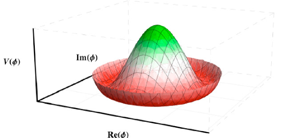
  Figure 1: The Mexican hat potential for $V=\Bigl{(}a-b\,|\phi|^{2}\Bigr{)}^{2}$ with $a,b\geq 0$. From Ref. [1].

  If $V(\phi,\phi^{*})=V(|\phi|^{2})$, then it is symmetric for $\phi\mapsto\exp(i\alpha)\phi$. If the potential is of the type

  $${V=a\,|\phi|^{2}+\ b\,|\phi|^{4}\forall a,b\geq 0,}$$ (9)

  then the minimum is at $\langle\phi\rangle=0$ (here $\langle\phi\rangle\equiv\langle 0|\phi|0\rangle$ denotes the vacuum expectation value (VEV) of the field $\phi$). The vacuum state is then also symmetric under the symmetry since the origin is invariant. However if the potential is of the form

  $$V=\Bigl{(}a-b\,|\phi|^{2}\Bigr{)}^{2}\forall a,b\geq 0,$$ (10)

  the symmetry of $V$ is lost in the ground state $\langle\phi\rangle\neq 0$. The existence of hidden symmetries is important for at least two reasons:

  • This is a natural way to introduce an energy scale in the system, determined by the non vanishing VEV. In particular, in the Standard Model, the electroweak scale $M_{\textrm{ew}}\sim 10^{2}$ GeV defines the basic scale of mass for the particles of the standard model, the electroweak gauge bosons and the matter fields, through their Yukawa couplings, obtain their mass from the VEV.

  • The existence of hidden symmetries implies that the fundamental symmetries of nature may be larger than is apparent. This is because the only manifest symmetries we can observe are the symmetries of the vacuum we live in and not those of the full underlying theory. This opens-up an essentially unlimited resource to consider physical theories with an indefinite number of symmetries even though they are not explicitly realised in nature. The standard model is one typical example and supersymmetry and theories of extra dimensions are further examples.

1.4.1 The Standard Model

The Standard Model is well defined and currently well confirmed by experiments. It is based on the two classes of symmetry:

• space-time symmetry: Poincaré symmetry in 4 dimensions.

• internal symmetry: gauged $G_{SM}$=SU(3)${}_{c}\times$SU(2)${}_{L}\times$U(1)_Y symmetry, where SU(3)_c defines the strong interactions. SU(2)${}_{L}\times$U(1)_Y is spontaneously broken by the Higgs mechanism to U(1)_em. The gauge fields are spin-1 bosons, for example the photon $A^{\mu}$, or gluons $G^{a=1,\ldots,8}$. Matter fields (quarks and leptons) have spin 1/2$\hbar$ and come in three ‘families’ (successively heavier copies). The Higgs boson (a particle has been discovered at the LHC whose properties are consistent with the Standard Model Higgs boson) is the spin zero particle that spontaneously breaks the SU(2)${}_{L}\times$U(1)_Y. The $W^{\pm}$ and $Z^{0}$ bosons get a mass via the Higgs mechanism and therefore the weak interactions are short range. This is also the source of masses for all quarks and leptons. The sub-index $L$ in $SU(2)_{L}$ refers to the fact that the Standard Model does not preserve parity and differentiates between left-handed and right-handed particles. In the Standard Model only left-handed fermions (and right-handed anti-fermions) transform non-trivially under $SU(2)_{L}$. The gauge particles have all spin $s=1\hbar$ and mediate each of the three forces: photons ($\gamma$) for $U(1)$ electromagnetism, gluons for $SU(3)_{C}$ of strong interactions, and the massive $W^{\pm}$ and $Z^{0}$ bosons for the weak interactions.

1.5 Problems of the Standard Model

The Standard Model is one of the cornerstones of all science and one of the great triumphs of the past century. It has been carefully experimentally verified in many ways, especially during the past 20 years. However, there are still some unresolved issues or mysteries:

• The hierarchy problem. The Higgs mass is $m_{h}\approx 125$ GeV, whereas the gravitational scale is $M_{Planck}\sim\sqrt{G}\sim 10^{19}$ GeV. The ‘hierarchy problem’ is: why is $m_{h}/M_{Planck}\sim 10^{-17}$ so much smaller than 1? In a fundamental theory, one might expect them to be the same order. In QFT, one sees that quantum corrections (loops) to $m_{h}$ are expected to be of order of the heaviest scale in the theory divided by $4\pi$. The question of why the hierarchy is stable with respect to the quantum corrections is called the technical hierarchy problem, and is arguably the main motivation for weak-scale supersymmetry.

• The cosmological constant ($\Lambda$) problem: probably the biggest unsolved problem in fundamental physics. $\Lambda$ is the energy density of free space time. The cosmological constant problem is: Why is $(\Lambda/M_{Planck})^{4}\sim 10^{-120}\ll 1$?

• The Standard Model has around 20 parameters, which must be measured then set ‘by hand’. Many consider that a more satisfying fundamental theory would relate all of these parameters to less (or ideally one) fundamental parameter.

• What particle constitutes the inferred cold dark matter in the universe? It is not contained in the Standard Model. Planck and large scale structure data favour a cosmological constant-cold dark matter model, where approximately 22$\%$ of the universe’s energy budget lies in dark matter, only 4$\%$ in ordinary matter, and some 74$\%$ in mysterious dark energy. Neutrinos constitute a hot component of dark matter (since they are relativistic when they decouple from the thermal plasma i.e. they smooth density perturbations in the early universe on smaller scales), so they are not good candidates.

  

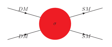
  Figure 2: For time $t\rightarrow$ (i.e. time increasing toward the right), this describes annihilation: once the particle physics model is set, a calculation tells us how much is thermally produced in the early universe. This also is a diagram for dark matter indirect detection, for example by dark matter collecting in the core of the sun and annihilating into neutrinos which could be detected by the IceCube experiment. For $t\leftarrow$, the diagram depicts collider production at (e.g.) the LHC, whereas for $t\uparrow$, it’s direct detection, where dark matter colliding with heavy nuclei may produce measurable nuclear recoils.

• The anomalous magnetic moment of the muon: This is a particular interaction between the photon and the muon: the Dirac equation predicts a muon magnetic moment

  $${\vec{M}=g_{\mu}\frac{e}{2m_{\mu}}\vec{S},}$$ (11)

  and at tree level, $g_{\mu}=2$. However, it can be measured very precisely by storing muons in a ring with magnetic fields, then measuring the precession frequency of their spins. The ‘anomalous’ part comes from loops involving various particles. Defining ${a_{\mu}\equiv\frac{g_{\mu}-2}{2}}$ [2],

  

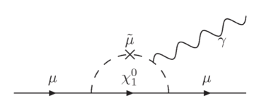
  Figure 3: Some SM contributions to the anomalous magnetic moment of the muon. From Ref. [2].

  $$a_{\mu}^{\textrm{exp}} = 11659209.1(5.4)(3.3)\times 10^{-10},\qquad a_{\mu}^{\textrm{SM}}=11659180.3(4.2)(2.6)\times 10^{-10},$$

  $$\Rightarrow\Delta a_{\mu} = a_{\mu}^{\textrm{exp}}-a_{\mu}^{\textrm{SM}}=28.8(6.3)(4.9)\times 10^{-10},$$ (12)

  where the first number in brackets labels the statistical error and the second the systematic error. The measurement of $(g-2)_{\mu}$ thus differs with the SM prediction at around the $\sim 3.6\sigma$ level (and has done for some 20 years). There should be a new more accurate measurement from the Muon $g-2$ experiment at the Fermilab collider in 2017. If one adds new particles to the SM, it is possible that they could travel in loops in diagrams similar to those in Fig. 3, and introduce a non-standard contribution to explain the discrepancy between the SM prediction and the SM measurement.

We wish to find extensions that could solve some or all of the problems mentioned above in order to generalise the Standard Model. Experiments are a traditional way of making progress in science. We need experiments to explore energies above the currently attainable scales and discover new particles and underlying principles that generalise the Standard Model. This approach is of course being followed at the LHC. The LHC will explore physics at the TeV scale, an interesting and important régime for new physics beyond the Standard Model. Notice that directly exploring energies closer to the Planck scale $M_{Planck}\approx 10^{19}$ GeV is out of the reach for many years to come.

1.5.1 The technical hierarchy problem

The Planck mass $M_{\textrm{pl}}\approx 10^{19}$ GeV is an energy scale associated with gravity and the electroweak scale $M_{\textrm{ew}}\approx 10^{2}$ GeV is an energy scale associated with the electroweak symmetry breaking scale of the Standard Model. The hierarchy problem involves these two scales being so different in magnitude. Actually the problem can be formulated in two parts:

• Why is $M_{\textrm{ew}}\ll M_{\textrm{pl}}$ at tree level? This question is known as ‘the hierarchy problem’. There are many solutions, once the SM is extended.

• Once we have solved (i), we ask why is the hierarchy stable under quantum corrections? This is the ‘technical hierarchy problem’ and does not have many full/effective solutions, aside from supersymmetry (SUSY).

Let us now think some more about the technical hierarchy problem. In the Standard Model we know that:

• Vector bosons are massless due to gauge invariance, that means, a direct mass term for the gauge particles $M^{2}A_{\mu}A^{\mu}$ is not allowed by gauge invariance ($A_{\mu}\rightarrow A_{\mu}+\partial_{\mu}\alpha$ for a $U(1)$ field, for example).

• Chiral fermion masses $m\bar{\psi}_{L}\psi_{R}$ are also forbidden for all quarks and leptons by gauge invariance (because, for example, $\psi_{L}$ and $\psi_{R}$ have different hypercharges). Recall that these particles receive a mass only through the Yukawa couplings to the Higgs (e.g. $H\bar{\psi}_{L}\psi_{R}$ giving a Dirac mass to $\psi$ after $H$ gets a non-zero value).

• The Higgs boson is the only fundamental scalar particle in the Standard Model. There is no symmetry banning its mass term $m_{h}^{2}H^{\dagger}H$ in the Standard Model Lagrangian. If the heaviest state in the theory has a mass squared of $\Lambda^{2}$, loops give corrections of order $\Lambda^{2}/(16\pi^{2})$ to the scalar mass squared. The corrections come from both bosons and fermions running in loops, for example:

  $$\begin{picture}(120.0,32.0)(0.0,0.0)\put(0.0,-30.0){\includegraphics[width=120.0pt]{mh}} \end{picture}\sim{-\frac{a\lambda^{2}}{16\pi^{2}}\int\frac{d^{n}k}{k^{2}-m_{F}^{2}}+\ldots},$$ (13)

  where $a$ is some dimensionless ${\mathcal{O}}(1)$ constant. The quantum correction to the Higgs mass from this diagram are:

  $${{m_{h}^{phys}}^{2}=({125~{}\mbox{GeV}/c^{2}})^{2}={m_{h}^{tree}}^{2}+\mathcal{O}({m_{F}^{2}}/(16\pi^{2})).}$$ (14)

  Experimentally, the Higgs mass is measured to be $m_{h}\approx 125$ GeV. The Standard Model is considered to be unnatural since the loop corrections are typically much larger: the largest are expected to be $\sim{\mathcal{O}}(10^{17})$ GeV. Therefore even if we start with a tree-level Higgs mass of order the electroweak scale, loop corrections would bring it up to almost the highest scale in the theory: $\Lambda/(4\pi)$, since we expect $m_{F}\sim{\mathcal{O}}(\Lambda)$. This would ruin the hierarchy between large and small scales. It is possible to adjust or “fine tune” the loop corrections such as to keep the Higgs light, but this would require cancellations between the apparently unrelated tree-level and loop contributions to some 15 significant figures. This fine tuning is considered unnatural and an explanation of why the Higgs mass (and the whole electroweak scale) can be naturally maintained to be hierarchically smaller than the Planck scale or any other large cutoff scale $\Lambda$ is required.

1.5.2 Modifications of the Standard Model

In order to go beyond the Standard Model we can follow several avenues, for example:

• Add new particles and/or interactions (e.g. a dark matter particle).

• More symmetries. For example,

• Internal symmetries, for example grand unified theories (GUTs) in which the symmetries of the Standard Model are themselves the result of the breaking of a yet larger symmetry group:

  $$G_{\textrm{GUT}}\stackrel{{\scriptstyle M\approx 10^{16}\textrm{GeV}}}{{\longrightarrow}}G_{\textrm{SM}}\stackrel{{\scriptstyle M\approx 10^{2}\textrm{GeV}}}{{\longrightarrow}}SU(3)_{c}\times U(1)_{Y},$$ (15)

  Let’s take one of the simplest examples, $G_{\textrm{GUT}}=SU(5)$:

  $$\underline{5} = \left(\begin{array}[]{c}{d}\\ {d}\\ {d}\\ e^{+}\\ \bar{\nu}_{e}\\ \end{array}\right)_{R},\qquad\underline{10}=\left(\begin{array}[]{ccccc}0&{\bar{u}}&{-\bar{u}}&{-u}&{-d}\\ &0&{\bar{u}}&{-u}&{d}\\ &&0&{-u}&{d}\\ &&&0&e^{+}\\ &&&&0\\ \end{array}\right)_{L}.$$ (26)

  (The $\underline{10}$ is an anti-symmetric matrix; we have omitted the lower left-hand half of it because the entries are simply related to those above the diagonal). Thus, we see how quarks and leptons become unified within multiplets of $G_{\textrm{GUT}}$.

  

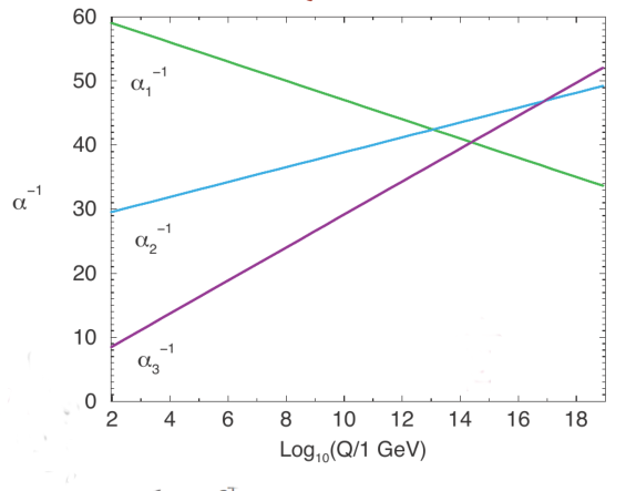
  Figure 4: Gauge unification doesn’t work in the Standard Model: the three gauge couplings $\alpha_{1},\alpha_{2},\alpha_{3}$ should all unify at a single renormalisation scale $Q$. One needs to add some additional particles of mass below $10^{14}$ GeV in order to make this work. Experiments (LEP and LHC experiments, for example) fix the gauge couplings at the left-hand side of the figure, and renormalisation within QFT is used to evolve them to the right. From Ref. [2].

  The GUT proposal is very elegant because it unifies, in one single symmetry, the three gauge interactions of the Standard Model. It leaves unanswered most of the open questions above, except for the fact that it reduces the number of independent parameters due to the fact that there is only one gauge coupling at large energies. This is expected to “run” at low energies and give rise to the three different couplings of the Standard Model (one corresponding to each group factor). Unfortunately, with our present precision understanding of the gauge couplings and spectrum of the Standard Model, the running of the three gauge couplings does not unify at a single coupling at higher energies but they cross each other at different energies: see Fig. 4. Because leptons and quarks are unified within GUT multiplets, they predict e.g. $m_{e}(M_{GUT})=m_{d}(M_{GUT})$, which also doesn’t work, and in practice further model building is required.

  GUTs have heavy $X$ and $Y$ gauge boson particles of order the gauge unification scale, which arise from a GUT Higgs mechanism (in a completely analogous way to the way in which the $W^{\pm}$ and $Z^{0}$ bosons acquire their mass).They predict proton decay, which isn’t observed at super-Kamiokande. The current constraint from super-Kamiokande is that the proton lifetime $\tau_{p\rightarrow e^{+}\pi^{0}}>10^{34}$ years.

  

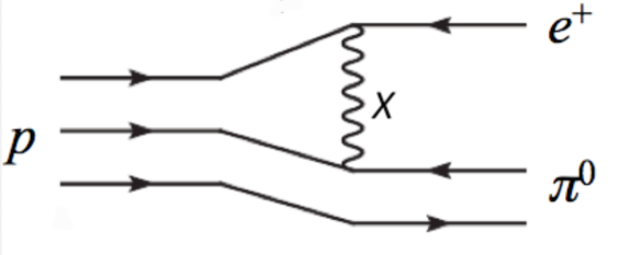
  Figure 5: Example $p\rightarrow e^{+}\pi^{0}$ process from GUTs. From Ref. [2].

  However, estimating $M_{GUT}\sim 10^{15}$ GeV from Fig. 4, we predict, for ordinary GUTs, a proton lifetime of

  $${\tau\approx\frac{M_{GUT}^{4}}{\alpha^{2}m_{p}^{5}}=4.5\times 10^{29\pm 1.7}\textrm{~{}years}},$$ (27)

  which easily is in contravention of the Super Kamiokande bound.

• Supersymmetry. For a phenomenological review of supserymmetry, see Ref. [3]. Supersymmetry is an external, or space-time, symmetry. Supersymmetry solves the technical hierarchy problem due to cancellations between the contributions of bosons and fermions to the electroweak scale, defined by the Higgs mass. Combined with the GUT idea, it also solves the unification of the three gauge couplings at one single point at larger energies. Supersymmetry also provides the most studied example for dark matter candidates. Moreover, it provides well defined QFTs in which the régime of strong coupling can be better studied than in non-supersymmetric models.

• Extra spatial dimensions. More general space-time symmetries open up many more interesting avenues for investigation. These can be of two types. First we can add more dimensions to space-time, extending the Poincaré symmetries of the Standard Model and the general coordinate transformations of general relativity. This is the well known Kaluza Klein theory in which our observation of a 4 dimensional universe is only due to the fact that we have limitations about “seeing” other dimensions of space-time that may be hidden to our observations. In recent years this has been extended to the brane world scenario in which our 4 dimensional universe is only a brane or surface inside a higher dimensional universe. These ideas lead to a different perspective on the hierarchy problem and also may help unify internal and space-time symmetries.

• Beyond QFT: A QFT with Supersymmetry and extra dimensions does not address the problem of quantising gravity. For this purpose, the current best hope is string theory which goes beyond the basic framework of QFT. It so happens that for its consistency, string theory requires supersymmetry and extra dimensions.

1.6 Supersymmetry algebra

1.6.1 History of supersymmetry

• In the 1960’s, the study of strong interactions lead to the discovery of many hadrons. These were successfully organised into multiplets of $SU(3)_{f}$, the $f$ referring to flavour. This procedure was known as the eight fold way of Gell-Mann and Neeman. Questions arose about bigger multiplets including particles of different spins.

• In a famous No-go theorem (Coleman, Mandula 1967) said that the most general symmetry of the $S$ - matrix (which still has non-trivial scattering) is Poincaré $\times$ internal. The implication is that there is no symmetry that mixes up the internal and external symmetries in a non-trivial way, or that mixes particles of different spin, and still has scattering.

• Golfand and Licktman (1971) extended the Poincaré algebra to include spinor generators $Q_{\alpha}$, where $\alpha=1,2$.

• Ramond, Neveu-Schwarz, Gervais, Sakita (1971) derived supersymmetry in 2 dimensions (from string theory).

• Wess and Zumino (1974) wrote down supersymmetric field theories in 4 dimensions. They opened the way for many other contributions to the field. This is often seen as the actual starting point for the systematic study of supersymmetry.

• Haag, Lopuszanski, Sohnius (1975): generalised the Coleman Mandula theorem to show that the only non-trivial quantum field theories have a symmetry group of super Poincaré group in a direct product with internal symmetries.

1.6.2 Graded algebra

The Poincaré algebra consists of commutation relations between 4-momentum operators $P^{\mu}$ (generating translations in space and time) and $M^{\mu\nu}$, generating Lorentz boosts and rotations. Particles of the Standard Model are all irreducible representations of the Poincaré group.

To implement supersymmetry, we extend the Poincaré algebra non-trivially. The Coleman Mandula theorem stated that in 3$+$1 dimensions, one cannot do this in a non-trivial way and still have non-zero scattering amplitudes. In other words, there is no non-trivial mix of Poincaré and internal symmetries with non-zero scattering except for the direct product

Poincaré $\times$ internal.

However (as usual with no-go theorems) there was a loop-hole because of an implicit axiom: the proof only considered “bosonic generators”.

We wish to turn bosons into fermions, thus we need to introduce a fermionic generator $Q$. Heuristically:

$$Q|\mbox{boson}\rangle\propto|\mbox{fermion}\rangle,\qquad Q|\mbox{fermion}\rangle\propto|\mbox{boson}\rangle.$$

For this, we require a graded algebra - a generalisation of Lie algebra. If $O_{a}$ is an operator of an algebra (such as a group generator), a graded algebra is

$$O_{a}O_{b}-(-1)^{\eta_{a}\eta_{b}}O_{b}O_{a}=iC^{e}_{ab}O_{e},$$ (28)

where $\eta_{a}=0$ if $O_{a}$ is a bosonic generator, and $\eta_{a}=1$ if $O_{a}$ is a fermionic generator.

For supersymmetry, the bosonic generators are the Poincaré generators $P^{\mu}$, $M^{\mu\nu}$ and the fermionic generators are $Q_{\alpha}^{A}$, $\bar{Q}_{\dot{\alpha}}^{A}$, where $A=1,\ldots,N$. In case $N=1$ we speak of a simple supersymmetry (SUSY), in the case $N>1$, of an extended SUSY. Here, we will only discuss the more immediately phenomenologically relevant case of $N=1$.

2 Introducing the minimal supersymmetric standard model (MSSM)

The MSSM is based on $SU(3)_{C}\times SU(2)_{L}\times U(1)_{Y}\times(N=1\textrm{~{}SUSY})$. We must fit all of the experimentally discovered field states into $N=1$ ‘super multiplets’: just as quarks are 3 dimensional representations of $SU(3)$ (i.e. one has a red, blue and green quark all within one multiplet), the MSSM fits all of its particles into super multiplets, whose types are:

• Chiral super multiplets: These contain a chiral left-handed fermion and a complex scalar.

• Vector super multiplets: These contain a spin 1$\hbar$ vector boson and a spin 1/2$\hbar$ Majorana fermion.

Super multiplets are formally built up from the algebra (we omit such technical details from these lectures). Since the symmetry group is a direct product between SUSY and the SM gauge symmetries, one can perform a SUSY transformation without changing the gauge quantum numbers of the super multiplet. Spin 1$\hbar$ vector bosons (e.g. the gluon) must be in the adjoint representation (for $SU(3)$ this has eight colour states) in order to make a renormalisable QFT, therefore the vector super multiplets must be in the adjoint representation. Thus, the spin 1/2$\hbar$ copy must also be in the adjoint representation (thus, from our example, we predict eight colour states of spin 1/2$\hbar$ fermions: the ‘gluinos’). Supersymmetry imposes that the two partners $\tilde{f}_{L,R}$ and $F$ of the super multiplet should couple with the same strengths as each other to other particles, and it also imposes that they should have the same mass as each other. Since

$$m_{\tilde{f}_{L,R}}^{2}=m_{F}^{2},$$ (29)

and the scalars $\tilde{f}_{L,R}$ and the fermion $F$ couple to the Higgs field $h$ with the same strength coupling $\lambda$:

$$\begin{picture}(280.0,50.0)(30.0,-40.0)\put(100.0,0.0){\begin{picture}(200.0,20.0)(0.0,0.0)\put(-30.0,-60.0){\includegraphics[width=100.0pt]{sc}} \end{picture}} \put(210.0,0.0){\begin{picture}(200.0,20.0)(0.0,0.0)\put(-30.0,-70.0){\includegraphics[width=130.0pt]{mh}} \end{picture}} \put(175.0,-30.0){+}\end{picture}\sim{\mathcal{O}\left(\frac{m_{h}^{2}\log(M_{Z}/m_{F})}{16\pi^{2}}\right)}.$$ (30)

Even if $F$ is a very heavy field associated with the highest scale of new physics, Eq. 30 does not present a huge correction to $m_{h}^{2}$: it is a usual loop-level correction, adding a few percent. The really huge corrections from Eq. 14 $\propto m_{F}^{2}$ have been cancelled between the two diagrams in Eq. 30. This is how supersymmetry solves the technical hierarchy problem.

Eq. 29 is not realised in nature (no one has seen a scalar version of the electron with the same mass as it, for example) and so we must bear in mind that supersymmetry must eventually be broken. However, we only wish to break it in a way that preserves it as a solution to the technical hierarchy problem: in specific models of supersymmetry breaking this can be done, but the coupling relations (that superpartners couple to other fields with the same strength as their SM partners) remain valid even after SUSY breaking. In particular, Eqs. 29 and 30 become

$$m_{\tilde{f}_{L,R}}^{2}=m_{F}^{2}+\Delta m^{2},$$ (31)

whilst the scalars $\tilde{f}_{L,R}$ and the fermion $F$ still couple to the Higgs field $h$ with the same strength coupling $\lambda$:

$$\begin{picture}(280.0,50.0)(30.0,-40.0)\put(100.0,0.0){\begin{picture}(200.0,20.0)(0.0,0.0)\put(-30.0,-60.0){\includegraphics[width=100.0pt]{sc}} \end{picture}} \put(210.0,0.0){\begin{picture}(200.0,20.0)(0.0,0.0)\put(-30.0,-70.0){\includegraphics[width=130.0pt]{mh}} \end{picture}} \put(175.0,-30.0){+}\end{picture}\sim{\mathcal{O}\left(\frac{m_{h}^{2}\log(M_{Z}/m_{F})+\Delta m^{2}}{16\pi^{2}}\right)}.$$ (32)

Thus, as long as the splitting between the particles in a super multiplet is small, and as long as certain SUSY relations are preserved (such as the coupling of the Higgs field to the scalar and fermionic components of a super multiplet being equal), one still obtains only reasonable corrections to the Higgs mass squared, even if the fields $F$ and $\tilde{f}_{L,R}$ are very heavy. The fact that we require $\Delta m^{2}/(16\pi^{2})$ to be not much larger than $m_{h}^{2}=(125\textrm{~{}GeV})^{2}\Rightarrow\Delta m^{2}<{\mathcal{O}}(1\textrm{~{}TeV}^{2})$. This is then the main argument for why supersymmetric partners of SM particles should not be much heavier than the TeV scale, because otherwise its correction to the Higgs mass would be too large. Given that the LHC currently operators at a centre of mass energy of 13 TeV, this implies that there ought to be enough energy to pair produce such sparticles.

2.1 Particles

First of all, we have vector superfields containing the Standard Model gauge bosons. We write their representations under $(SU(3)_{C},\ SU(2)_{L},\ U(1)_{Y})$ as (pre-Higgs mechanism):

• gluons/gluinos

  $$G=(8,1,0)$$

• $W$ bosons/winos

  $$W=(1,3,0)$$

• $B$ bosons/gauginos

  $$B=(1,1,0),$$

  which contains the gauge boson of $U(1)_{Y}$.

Secondly, there are chiral superfields containing Standard Model matter and Higgs fields. Since chiral superfields only contain left-handed fermions, we place charge conjugated, i.e. anti right handed fermionic fields (which are actually left-handed), denoted by ^c ($\{i,j,k\}\in\{1,2,3\}$ are family indices):

• (s)quarks: lepton number $L=0$, whereas baryon number $B=1/3$ for a (s)quark, $B=-1/3$ for an anti-quark.

  $$\underbrace{Q_{i}=\left(3,2,\tfrac{1}{6}\right)}_{\textrm{left-handed}},\underbrace{{u}_{i}^{c}=\left(\bar{3},1,-\tfrac{2}{3}\right),{d}_{i}^{c}=\left(\bar{3},1,\tfrac{1}{3}\right)}_{\textrm{anti (right-handed)}}$$

• (s)leptons $L=1$ for a lepton, $L=-1$ for an anti-lepton. $B=0$.

  $$\underbrace{L_{i}=\left(1,2,-\tfrac{1}{2}\right)}_{\textrm{left-handed}},\underbrace{{e}_{i}^{c}=\left(1,1,+1\right)}_{\textrm{anti (right-handed)}}$$

• Higgs bosons/higgsinos: $B=L=0$.

  $$H_{2}=\left(1,2,\tfrac{1}{2}\right),H_{1}=\left(1,2,\ -\tfrac{1}{2}\right)$$

  the second of which is a new Higgs doublet not present in the Standard Model. Thus, the MSSM is a two Higgs doublet model. The extra Higgs doublet is needed in order to avoid a gauge anomaly, and to give masses to down-type quarks and leptons.

Note that after the breaking of electroweak symmetry (see the Standard Model course), the electric charge generator is $Q=T_{3}^{SU(2)_{L}}+Y/2$. Baryon and lepton number correspond to multiplicative discrete perturbative symmetries in the SM, and are thus conserved, perturbatively.

Chiral fermions may generate an anomaly in the theory, as shown by Fig. 6. This is where a symmetry that is present in the tree-level Lagrangian is broken by quantum corrections. Here, the symmetry is $U(1)_{Y}$: all chiral fermions in the theory travel in the loop, and yield a logarithmic divergence proportional to

$$A\equiv\sum_{LH\ f_{i}}Y_{i}^{3}-\sum_{RH\ f_{i}}Y_{i}^{3}$$ (33)

multiplied by some kinematic factor which is the same for each fermion. If $A$ is non-zero, one must renormalise the diagram away by adding a $B_{\mu}B_{\nu}B_{\rho}$ counter term in the Lagrangian. But this breaks $U(1)_{Y}$, meaning that $U(1)_{Y}$ would not be a consistent symmetry at the quantum level.

Figure 6: Anomalous Feynman diagrams proportional to Tr$\{Y^{3}\}$. The sum of them must vanish for $U(1)_{Y}$ to be a valid symmetry at the quantum level. Hyper-charged chiral fermions $f$ travel in the loop contributing to a three-hypercharge gauge boson $B$ vertex. From Ref. [1].

Fortunately, $A=0$ for each fermion family in the Standard Model. Contributions are from (the factors of 3 are from the different colours of the quarks, whereas the factors of 2 come from the different $SU(2)_{L}$ degrees of freedom):

$$\underbrace{3\times 2\times(\frac{1}{6})^{3}}_{Q_{L}}+\underbrace{3\times(-\frac{2}{3})^{3}}_{u_{R}^{c}}+\underbrace{3\times(\frac{1}{3})^{3}}_{d_{R}^{c}}+\underbrace{2\times(-\frac{1}{2}))^{3}}_{L_{L}}+\underbrace{1^{3}}_{e_{R}^{c}}=0.$$

In SUSY, we add the Higgsino doublet $\tilde{H}_{1}$, which yields a non-zero contribution to $A$. This must be cancelled by another Higgsino doublet with opposite $Y$: $\tilde{H}_{2}$.

There is another special super multiplet sometimes considered to be part of the MSSM with $B=L=0$. This is the gravity super multiplet, with the spin $2\hbar$ graviton and a spin $3/2\hbar$ gravitino. Usually, after SUSY breaking (see later), the only component of the gravitino that couples with non-negligible strength is its spin $1/2\hbar$ component.

$$G=\left(1,1,1\right)$$

2.2 Interactions

• Gauge couplings are renormalised, which ends up giving them renormalisation scale dependence, which matches onto dependence upon the energy scale at which one is probing them:

  $$\mu\frac{dg_{a}(\mu)}{d\mu}=\beta_{a}g_{a}^{3}(\mu),\Rightarrow g_{a}^{-2}(\mu)=g_{a}^{-2}(\mu_{0})-2\beta_{a}\ln\frac{\mu}{\mu_{0}}$$ (34)

  where $\beta_{a}$ is a constant determined by which particles travel in the loop in the theory. For ordinary QCD it is $\beta_{3}=-7/(16\pi^{2})$ whereas for the MSSM, it is $\beta_{3}=-3/(16\pi^{2})$ because of additional contributions from squarks and gluinos to the loops, as in Fig. 7.

  

  Figure 7: Example Feynman diagrams leading to renormalisation of the strong coupling constant $g_{3}$. The left-hand diagram renormalises the QCD gauge coupling in the Standard Model, whereas in the MSSM, we have additional contributions from supersymmetric particles such as the one on the right-hand side with gluinos in the loop. There are other contributing diagrams, some involving loops of quarks and squarks, for instance.

  Eq. 34 is used to extrapolate gauge couplings measured at some energy scale $\mu_{0}$ (often taken to be $M_{Z}$, from LEP constraints) to some other scale $\mu$. With the SUSY contributions in the MSSM, the gauge couplings almost meet at a renormalisation scale $E\approx 2\times 10^{16}$ GeV (see Fig. 8), whereas with just the Standard Model contributions, they do not meet each other at all: see Fig. 4. The meeting of the gauge couplings is a necessary condition for a Grand Unified Theory, which only has one gauge coupling (above $M_{GUT}\approx 2\times 10^{16}$ GeV). $\alpha_{1}(M_{Z})$ and $\alpha_{2}(M_{Z})$ are both known with high accuracy from the LEP experiments, so we can use them to predict $M_{GUT}\sim 10^{16}$ GeV and $\alpha_{s}(M_{Z})=0.129\pm 0.002$. The experimental determination of $\alpha_{s}(M_{Z})=0.119\pm 0.002$, so the naive prediction is some $5\sigma$ out. However, this small difference is easily explained by GUT threshold corrections (for example because the $X$ or $Y$ bosons are a factor of a few lighter than $M_{GUT}$ and change the running near the GUT scale) in explicit GUT models.

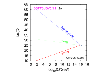
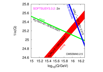
  Figure 8: Gauge unification in the MSSM: the thickness of the lines corresponds to the $2\sigma$ error bars. The right-hand panel shows a zoom of the unification region near $Q\sim 10^{16}$ GeV.

  Gauge couplings are renormalised, which ends up giving them renormalisation scale dependence, which matches onto dependence upon the energy scale at which one is probing them (one achieves a worse approximation in a truncated perturbation series by picking the renormalisation scale to be vastly different to the energy scales probed in some process): integrating both sides,

  $${\mu\frac{dg_{a}(\mu)}{d\mu}=\beta_{a}g_{a}^{3}(\mu),\Rightarrow g_{a}^{-2}(\mu)=g_{a}^{-2}(\mu_{0})-2\beta_{a}\ln\frac{\mu}{\mu_{0}}}$$ (35)

  where $\beta_{a}$ is a constant determined by which particles travel in the loop in the theory. For ordinary QCD it is $\beta_{3}=-7/(16\pi^{2})$ whereas for the MSSM, it is $\beta_{3}=-3/(16\pi^{2})$ because of additional contributions from squarks and gluinos to the loops.

• A ‘superpotential’ is like a Lagrangian energy density for SUSY theories: it encodes some of the interactions between the chiral superfields in a way that preserves SUSY. A superpotential term $W=\lambda\Phi^{3}$ for a chiral superfield $\Phi=(\varphi,\ \psi)$ encodes both a Yukawa interaction ${\mathcal{L}}=-\lambda\varphi\psi\psi$ and a scalar interaction ${\mathcal{L}}=-|\lambda|^{2}|\varphi|^{4}$, for example.

  We write down a superpotential containing all terms which are renormalisable and consistent with our symmetries. If one does this, one obtains two classes of terms, $W=W_{R_{p}}+W_{RPV}$. The terms in $W_{R_{p}}$ all conserve baryon number $B$ and lepton number $L$, whereas those in $W_{RPV}$ break either $B$ or $L$:

  $$W_{R_{p}} =(Y_{U})_{ij}\,Q_{i}\,H_{2}\,{u}^{c}_{j}+(Y_{D})_{ij}\,Q_{i}\,H_{1}\,{d}^{c}_{j}+Y_{E}\,L_{i}\,H_{1}\,{e}^{c}_{j}+\mu\,H_{1}\,H_{2}$$ (36)

  $$W_{RPV} =\lambda_{ijk}\,L_{i}\,L_{j}\,{e}^{c}_{k}+\lambda^{\prime}_{ijk}\,L_{i}\,Q_{j}\,{d}^{c}_{k}+\lambda^{\prime\prime}_{ijk}\,{u}^{c}_{i}\,{d}^{c}_{j}\,{d}^{c}_{k}+\kappa_{i}\,L_{i}\,H_{2},$$ (37)

  where we have suppressed gauge indices. Since superfields commute in $W$,

  $$H_{1}^{a}H_{1}^{b}\epsilon_{ab}=\frac{1}{2}(H_{1}^{a}H_{1}^{b}+H_{1}^{b}H_{1}^{a})\epsilon_{ab}=\frac{1}{2}H_{1}^{a}H_{1}^{b}(\epsilon_{ab}+\epsilon_{ba})=0$$ (38)

  The first three terms in $W_{R_{p}}$ correspond to standard Yukawa couplings and give masses to up quarks, down quarks and leptons, as we shall see. Writing $x=1,2,3$ as a fundamental $SU(3)$ index, $a,b=1,2$ as fundamental $SU(2)$ indices, the first term in $W_{R_{p}}$ becomes

  $$(Y_{U})_{ij}Q_{i}^{xa}H_{2}^{b}u^{c}_{jx}\epsilon_{ab}=(Y_{U})_{ij}[u_{L}^{x}H_{2}^{0}u^{c}_{jx}-d_{L}^{x}H_{2}^{+}u^{c}_{jx}].$$ (39)

  Once the neutral Higgs component develops a vacuum expectation value, $H_{2}^{0}\equiv(v_{2}+h_{2}^{0})/\sqrt{2}$, the first term becomes $(Y_{U})_{ij}v_{2}/\sqrt{2}u_{Li}^{x}u^{c}_{jx}+\ldots$, yielding a Dirac mass matrix $m_{u}\equiv(Y_{U})_{ij}v_{2}/\sqrt{2}$ for the up quarks. The down quark and lepton masses proceed in an analogous manner. The fourth term is a mass term for the two Higgs(ino) fields.

  If all of the terms in $W_{RPV}$ are present, the interaction shown in Fig. 9 would allow proton decay $p\rightarrow e^{+}+\pi^{0}$ within seconds because

  $$\Gamma(p\rightarrow e^{+}\pi^{0})\approx\frac{{\lambda^{\prime}}_{11k}^{2}{\lambda^{\prime\prime}}_{11k}^{2}}{16\pi^{2}{{\tilde{m}}_{d_{k}}}^{4}}{M_{p}^{5}},$$ (40)

  whereas experiments say that it should be $>10^{34}$ years. Alternatively, we could make the RPV couplings very small to make the proton long-lived, by imposing the implied bound on $\Gamma(p\rightarrow e^{+}\pi^{0})$:

  $$\lambda^{\prime}_{11k}\cdot\lambda^{\prime\prime}_{11k}\;<{10^{-27}}\left(\frac{{\tilde{m}}_{d_{k}}}{100\mbox{~{}GeV}}\right)^{2}.$$ (41)

  

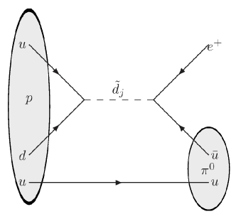
  Figure 9: Proton decay $p\rightarrow e^{+}\pi^{0}$ due to baryon- and lepton number violating interactions. Both $B$ and $L$ violating terms must be present for the proton to decay. The matrix element is proportional to ${\lambda^{\prime\prime}_{1j1}}^{*}\times{\lambda^{\prime}_{11j}}^{*}$.

  In order to forbid proton decay an extra symmetry should be imposed. One symmetry that works is a discrete multiplicative symmetry R parity defined as

  $$R\equiv(-1)^{3(B-L)+2S}=\left\{\begin{array}[]{l}+1:\textrm{Standard Model particles,}\qquad-1:\textrm{superpartners}\end{array}\right..$$ (42)

  It forbids all of the terms in $W_{RPV}$, but there exist other examples which only ban some subset.

R parity would have important physical implications:

• The lightest superpartner (LSP) is stable, because it is $R-$parity odd.

• Cosmological constraints then say that a stable LSP must be electrically and colour-neutral (higgsino, photino, zino). It is then a good candidate for cold weakly interacting dark matter.

• In colliders, the initial state is $R_{p}=+1$, implying that superparticles are produced in pairs. When a superparticle decays, it must decay to another (lighter) superparticle plus some standard model particles.

• One ends up with LSPs at the end of the decays. These do not interact with the detector, and hence appear as unbalanced or ‘missing’ momentum.

Note that the terms in $W_{RPV}$ can lead to Majorana fermion structure. For instance, $W=\lambda^{\prime\prime}_{112}u_{1}^{c}d_{1}^{c}d_{2}^{c}$: we take the $F-$ terms as usual in order to find the Lagrangian in terms of components:

$${\mathcal{L}}=\frac{1}{2}\left({\lambda^{\prime\prime}_{112}}\tilde{u}_{1}^{*}{d_{1}}_{R}^{\dagger}C{d_{2}}_{R}^{*}-({\lambda^{\prime\prime}_{112}})^{*}\tilde{u}_{1}{d_{1}}_{R}^{T}C^{*}{d_{2}}_{R}\right)$$

plus supersymmetric copies, where $C$ is the charge conjugation matrix and ^T denotes transpose.

RPV has several potential motivations and characteristics:

• It has many additional search possibilities

• Dark matter changes character: one loses the usual neutralino dark matter candidate. However, the SUSY breaking sector always contains other fields that may be used instead, for example the gravitino or hidden sector fields. Either of these two candidates is so weakly coupled that direct or indirect dark matter detection becomes extremely unlikely, although inference of its production at colliders is still possible.

• Neutrino masses and mixings are generated by the $L$ violating couplings in diagrams like those in Fig. 10, and the mechanism of their generation is potentially testable at the LHC (unlike, for example, the seesaw mechanism of producing neutrino masses).

  

  Figure 10: RPV generation of neutrino masses and mixings. Here, the dots show the $L$ violating RPV couplings.

2.3 Supersymmetry breaking in the MSSM

An operator called the supertrace treats bosonic and fermionic parts of a super multiplet differently. It is defined as

$${\rm STr}\bigl{\{}M^{2}\bigr{\}}\equiv\sum_{j}(-1)^{2j+1}\,(2j+1)\,m_{j}^{2}=0,$$ (43)

where $j$ represents the ‘spin’ of the particles in some super multiplet. This is generic for tree level directly broken SUSY. Thus, we cannot break supersymmetry directly in the MSSM, since it preserves ${\rm STr}\bigl{\{}M^{2}\bigr{\}}=0$. Applying this to the photon, say: $-3m_{\gamma}^{2}+2m_{\tilde{\gamma}}^{2}=0$, which would predict a massless photino that hasn’t been observed. Applying it to up quarks: $2m_{u}^{2}-m_{{\tilde{u}}_{L}}^{2}-m_{{\tilde{u}}_{R}}^{2}=0$, thus one up squark must be lighter than the up quark, again this hasn’t been observed. We introduce a hidden sector, which breaks SUSY and has its own fields (which do not directly interact with MSSM fields) and interactions, and an additional messenger sector to communicate the SUSY breaking to the observable sector fields:

$$\left(\begin{array}[]{c}\textrm{observable}\\ \textrm{sector, MSSM}\end{array}\right)\longleftrightarrow\left(\begin{array}[]{c}\textrm{messenger -}\\ \textrm{sector}\end{array}\right)\longleftrightarrow\left(\begin{array}[]{c}\textrm{hidden}\\ \textrm{sector}\end{array}\right).$$

This gets around the supertrace rule. There is typically an overall gauge group

$$\bigl{(}SU(3)\times SU(2)\times U(1)\bigr{)}\times G_{\cancel{\textrm{SUSY}}}\equiv G_{SM}\times G_{\cancel{\textrm{SUSY}}},$$

where the MSSM fields are singlets of $G_{\cancel{\textrm{SUSY}}}$ and the hidden sector fields are singlets of $G_{SM}$.

We have already seen several examples of SUSY breaking theories. One popular SUSY-breaking sector in the MSSM context is that of gaugino condensation: here, some asymptotically free gauge coupling $g$ becomes large at some energy scale $\Lambda$. $g$ will renormalise like Eq. 34 with some beta function coefficient. Solving the equation, with $g^{-2}(\Lambda)\rightarrow 0$, we obtain $\Lambda=M\exp[g^{-2}(M)/\beta]$. $M$ could be some large scale such as the string scale, $\sim 5\times 10^{17}$ GeV. It is easy to arrange for $\Lambda\ll M$ because of the exponential suppression. When the gauge coupling becomes large, and the theory becomes non-perturbative, one can obtain $\langle\tilde{g}\tilde{g}\rangle\sim{\mathcal{O}}(\Lambda^{3})$, breaking SUSY dynamically.

The SUSY breaking fields have couplings with the messenger sector, which in turn have couplings with the MSSM fields, and carry the SUSY breaking over to them. There are several possibilities for the messenger sector fields, which may determine the explicit form of SUSY breaking terms in the MSSM, including (note here that $M_{\cancel{\textrm{SUSY}}}$ is the SUSY breaking in the hidden sector, whereas $\Delta m$ is the SUSY breaking that ends up in the MSSM fields):

• gravity mediated $\cancel{\textrm{SUSY}}$

  If the mediating field couples with gravitational strength to the standard model, the couplings are suppressed by the inverse Planck mass $M_{\textrm{pl}}$, the natural scale of gravity. The SUSY breaking mass splitting between MSSM particles and superparticles, $\Delta m$, becomes

  $$\Delta m=\frac{M_{\cancel{\textrm{SUSY}}}^{2}}{M_{\textrm{pl}}}.$$ (44)

  We want $\Delta m\approx 1\textrm{TeV}$ and we know that $M_{\textrm{pl}}\approx 10^{19}\textrm{GeV}$, so

  $$M_{\cancel{\textrm{SUSY}}}=\sqrt{\Delta m\cdot M_{\textrm{pl}}}\approx 10^{11}\textrm{GeV}.$$ (45)

  The gravitino gets a mass $m_{\frac{3}{2}}$ of $\Delta m$ order TeV from the ‘super Higgs mechanism’.

  

  Figure 11: Gaugino condensation and supergravity mediated SUSY breaking. From Ref. [1].

• gauge mediated $\cancel{\textrm{SUSY}}$

  Messenger fields are charged under both $G_{SM}$ and $G_{\cancel{\textrm{SUSY}}}$. Gauge loops transmit SUSY breaking to the MSSM fields. Thus, $\Delta m\sim M_{\cancel{\textrm{SUSY}}}/(16\pi^{2})$ is required to be of order TeV. In this case, the gravitino mass $m_{\frac{3}{2}}\sim\frac{M^{2}_{\cancel{\textrm{SUSY}}}}{M_{\textrm{pl}}}\sim\textrm{eV}$ and the gravitino is the LSP.

• anomaly mediated $\cancel{\textrm{SUSY}}$

  In this case, the auxiliary fields of supergravity get a vacuum expectation value. The effects are always present, but suppressed by loop factors. They may be dominant if the tree-level contribution is suppressed for some reason.

Each of these scenarios has phenomenological advantages and disadvantages and solving their problems is an active field of research. In all scenarios, the Lagrangian for the observable sector has contributions

$${\cal L}={\cal L}_{\textrm{SUSY}}+{\cal L}_{\cancel{\textrm{SUSY}}}.$$ (46)

In the second term, we write down all renormalisable symmetry invariant terms which do not reintroduce the hierarchy problem. They are of the form (where $i$ and $j$ label different fields):

$$\framebox{$\displaystyle{\cal L}_{\cancel{\textrm{SUSY}}}=\underbrace{m^{2}_{ij}\,\varphi^{*}_{i}\,\varphi_{j}+{m^{\prime}}^{2}_{ij}(\varphi_{i}\varphi_{j}+h.c.)}_{\textrm{scalar masses}}+\left(\underbrace{\frac{1}{2}M_{\lambda}\,\lambda\lambda}_{\textrm{gaugino masses}}+\underbrace{A_{ijk}\,\varphi_{i}\varphi_{j}\varphi_{k}}_{\textrm{trilinear couplings}}+h.c.\right).$}$$ (47)

$M_{\lambda},{m^{\prime}}^{2}_{ij},{m}_{ij}^{2},A_{ijk}$ are called soft SUSY breaking terms: they do not reintroduce quadratic divergences into the theory. Particular forms of SUSY breaking mediation can give relations between the different soft SUSY breaking terms. They determine the amount by which supersymmetry is expected to be broken in the observable sector, and the masses of the superparticles for which the LHC is searching.

Figure 12: An example of renormalisation in the MSSM using the program SOFTSUSY [4] to calculate the renormalisation. A particular high energy theory is assumed, which has GUT symmetry and implies that the gauginos are all mass degenerate at the GUT scale. The scalars (e.g the right-handed electron $Er$ and the left-handed squarks $Ql$) are also mass-degenerate at the GUT scale. Below the GUT scale though, the masses split and renormalise separately. When we are scattering at energies $\sim O(100)$ GeV, it is a good approximation to use the masses evaluated at that renormalisation scale $\mu\approx E$. We see that one of the Higgs mass squared parameters, $\mu^{2}+M_{Hu}^{2}$, becomes negative at the electroweak scale, triggering electroweak symmetry breaking.

Explicitly, we parameterise all of the terms that softly break SUSY in the $R_{p}$ preserving MSSM, suppressing gauge indices:

$${\mathcal{L}}_{R_{p}}^{{\cancel{\textrm{SUSY}}}} = (A_{U})_{ij}{\tilde{Q}}_{Li}H_{2}{\tilde{u}}_{Rj}^{*}+(A_{D})_{ij}{\tilde{Q}}_{Li}H_{1}{\tilde{d}}_{Rj}^{*}+(A_{E})_{ij}{\tilde{L}}_{Li}H_{1}{\tilde{e}}_{Rj}^{*}+$$

$${\tilde{Q}}_{Li}^{*}(m_{\tilde{Q}}^{2})_{ij}{\tilde{Q}}_{Lj}+{\tilde{L}}_{i}^{*}(m_{\tilde{L}}^{2})_{ij}{\tilde{L}}_{j}+{\tilde{u}}_{Ri}(m_{\tilde{U}}^{2})_{ij}{\tilde{u}}_{Rj}^{*}+{\tilde{d}}_{Ri}(m_{\tilde{D}}^{2})_{ij}{\tilde{d}}_{Rj}^{*}+{\tilde{e}}_{Ri}(m_{\tilde{E}}^{2})_{ij}{\tilde{e}}_{Rj}^{*}+$$

$$(m_{3}^{2}H_{1}H_{2}+h.c.)+m_{1}^{2}|H_{1}^{2}|+m_{2}^{2}|H_{2}|^{2}+\frac{1}{2}M_{3}\tilde{g}\tilde{g}+\frac{1}{2}M_{2}\tilde{W}\tilde{W}+\frac{1}{2}M_{1}\tilde{B}\tilde{B}.$$

Sometimes, $m_{3}^{2}$ is written as $\mu B$. Often, specific high scale models provide relations between these many parameters. For instance, the Constrained MSSM (which may come from some particular string theory or other field theory) specifies the constraints

$$M_{1} = M_{2}=M_{3}=:M_{1/2}$$

$$m_{\tilde{Q}}^{2} = m_{\tilde{L}}^{2}=m_{\tilde{U}}^{2}=m_{\tilde{D}}^{2}=m_{\tilde{E}}^{2}\equiv m_{0}^{2}I_{3}$$

$$m_{1}^{2} = m_{2}^{2}=m_{0}^{2}$$

$$A_{U} = A_{0}Y_{U},\ A_{D}=A_{0}Y_{D},\ A_{E}=A_{0}Y_{E}$$

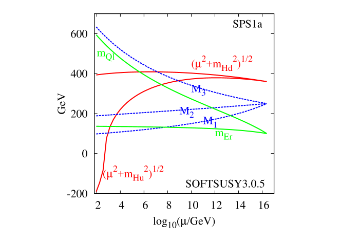
where $I_{3}$ is the 3 by 3 identity matrix. Thus in the ‘CMSSM’, we reduce the large number of free SUSY breaking parameters down to 3: $M_{1/2}$, $m_{0}$ and $A_{0}$. These relations hold at the GUT scale, and receive large quantum corrections, as Fig. 12 shows.

2.4 States after electroweak symmetry breaking

With two complex Higgs doublets, we count 8 real degrees of freedom. 3 of these are ‘eaten’ by the longitudinal components of the W^± and $Z^{0}$ bosons, leaving a total of five physical Higgs fields: two $CP-$even (in mass order) $h^{0},H^{0}$, one $CP-$odd $A^{0}$ and two charged Higgs’ $H^{\pm}$. The other SUSY particles that have identical quantum numbers under QED$\times$QCD mix after electroweak symmetry breaking: for example the bino, wino, and two neutral Higgsinos mix. Their mass eigenstates are called neutralinos, conventionally written in order of their masses $\chi^{0}_{1,2,3,4}$. $\chi_{1}^{0}$ typically has a special status in that is a good candidate for dark matter if it is the lightest supersymmetric particle and $R_{p}$ is conserved. The scalar partner of the left-handed top (called the ‘left-handed stop’) mixes with the right-handed stop to form two mass eigenstates: $\tilde{t}_{1,2}$. This analogously occurs for the sbottoms and staus as well. The charged Higgsinos mix with the winos to form mass eigenstates called ‘charginos’: $\chi^{\pm}_{1,2}$.

2.5 The Neutral Higgs Potential

Both Higgs’ of the MSSM acquire vacuum expectation values:

$$\left(\begin{array}[]{c}H_{1}^{0}\\ H_{1}^{-}\end{array}\right)\rightarrow\left(\begin{array}[]{c}v_{1}\\ 0\end{array}\right)\qquad\left(\begin{array}[]{c}H_{2}^{+}\\ H_{2}^{0}\end{array}\right)\rightarrow\left(\begin{array}[]{c}0\\ v_{2}\end{array}\right)\qquad$$ (48)

and to get the value of $M_{W}$ to match with experimental data, we require $v_{SM}=246$ GeV. In a two-Higgs doublet model, this leads to the following construction:

$\tan\beta$ is a parameter which changes the phenomenology of the model because the third family Yukawa couplings depend upon it, and they are comparatively large dimensionless couplings. The Yukawa terms from the MSSM superpotential are:

$${\mathcal{L}} = {h_{t}}\bar{t}_{L}H_{2}^{0}t_{R}+h_{b}\bar{b}_{L}H_{1}^{0}b_{R}+h_{\tau}\bar{\tau}_{L}H_{1}^{0}\tau_{R}+\textrm{H.c.}+\ldots$$ (49)

$$\Rightarrow\frac{m_{t}}{\sin\beta} = \frac{{h_{t}}v_{SM}}{\sqrt{2}},\qquad\frac{m_{b,\tau}}{\cos\beta}=\frac{h_{b,\tau}v_{SM}}{\sqrt{2}},$$ (50)

after electroweak symmetry breaking and the neutral components of Higgs’ are replaced by their vacuum expectation values: $H_{i}^{0}=(v_{i}^{0}+H_{i}^{0})/\sqrt{2}$.

Picking out only the terms involving the neutral Higgs fields $H_{1}^{0}$ and $H_{2}^{0}$, we have the neutral Higgs potential

$$V={(|\mu|^{2}+{m_{H_{2}}^{2}})|H_{2}^{0}|^{2}+(|\mu|^{2}+m_{H_{1}}^{2})|H_{1}^{0}|^{2})}{-\mu B(H_{2}^{0}H_{1}^{0}+\textrm{H.c.})}{+\frac{1}{8}(g^{2}+{g^{\prime}}^{2})(|H_{2}^{0}|^{2}-|H_{1}^{0}|^{2})^{2}.}$$ (51)

The vacuum minimises this potential with respect to both of the neutral components:

$${\frac{\partial V}{\partial H_{2}^{0}}=\frac{\partial V}{\partial H_{1}^{0}}=0}\Rightarrow\mu B={\frac{\sin 2\beta}{2}({\bar{m}}_{H_{1}}^{2}+{\bar{m}}_{H_{2}}^{2}+2\mu^{2}),}\mu^{2}={\frac{{\bar{m}}_{H_{1}}^{2}-{\bar{m}}_{H_{2}}^{2}\tan^{2}\beta}{\tan^{2}\beta-1}-\frac{M_{Z}^{2}}{2}}.$$ (52)

These two conditions should be used to eliminate two of the MSSM’s free parameters: often, $|\mu|$ and $B$ (although note that the sign of $\mu$ is physical and not determined by Eq. 52).

2.6 Pros and Cons of the MSSM

We start with a list of unattractive features of the MSSM:

• There are $\sim 100$ extra free parameters in the SUSY breaking sector, making for a complicated parameter space.

• Nearly all of this parameter space is ruled out by flavour physics constraints: SUSY particles could heavily mix in general, then this mixing could appear in loops and make the quarks mix in a flavour changing neutral current, upon which there are very strong experimental bounds. It could be that this clue is merely telling us that there is more structure to the MSSM parameter space, though (like in the CMSSM).

• The $\mu$ problem. $\mu$ in $W_{R_{p}}$ must be $<\mathcal{O}(1)$ TeV, since it contributes at tree-level to $m_{h}$. Why should this be, when in principle we could put it to be $\sim{\mathcal{O}}(M_{Pl})$, because it does not break any SM symmetries? (Note though that once it is set to be small at tree-level, SUSY protects it from large quantum corrections).

• As lower limits on sparticle masses increase, the extent to which SUSY solves the hierarchy problem decreases.

These SUSY problems can be solved with further model building.

Figure 13: Example one-loop diagram of sparticles contributing to $(g-2)_{\mu}$.

We close with an ordered list of weak-scale SUSY’s successes:

• SUSY solves the technical hierarchy problem.

• Gauge unification works.

• The MSSM contains a viable dark matter candidate, if $R_{p}$ is conserved.

• Electroweak symmetry breaks radiatively.

• A one-loop diagram involving sneutrinos and charginos (and one involving smuons and neutralinos: see Fig. 13) contribute to the anomalous magnetic moment of the muon, and may solve the discrepancy between SM predictions and experimental measurements in Eq. 12.

2.7 LHC Production of SUSY Particles

Figure 14: Picture of the production of sparticles at a 14 TeV LHC.

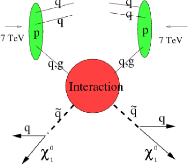
One turns the energy of the LHC beams into mass via $E=mc^{2}$, hoping to produce pairs (if $R_{p}$ is conserved) of SUSY particles that were too heavy to have been previously produced in lower energy machines. We show a schematic in Fig. 14: occasionally, high energy constituents of the proton (called ‘partons’: quarks or gluons) will collide, as in the figure. The idea is that these are most likely to make strongly interacting particles, all other things being equal (in the figure, we have the example of squark production). The rest of the broken protons typically will be boosted along the beam-line. The sparticles undergo subsequent decay (in the example in the figure, into a quark - which will form a jet of hadrons and a dark matter particle: the lightest neutralino). Since we have assumed $R_{p}$ to be conserved, the $\chi_{1}^{0}$ is stable but since it is weakly interacting, it passes through the rest of the detector without any interactions, stealing momentum from the collision. The decays of the initial pair of sparticles may be much more complex, going through cascade decays where at each stage there is a lighter sparticle and a SM particle produced. $R_{p}$ conserving SUSY provides an example of how any dark matter candidate that is light enough and that (perhaps indirectly) couples to protons can be produced in LHC collisions. Jets and missing transverse momentum $\vec{p}_{\mathrm{T}}^{\mathrm{miss}}$ (sometimes this is known under the misnomer ‘missing energy’) form a classic SUSY search, but also jets plus varying numbers of leptons (from sparticle cascade decays) plus missing transverse momentum form another well-studied class. There is a SUSY monojet signature [5], although sparticles would likely be found in one of the other production channels first because the monojet signature is due to a strong times an electroweak matrix element. In the case of gauge mediated SUSY breaking models, the lightest neutralino may decay into a gravitino plus a photon, or a $Z^{0}$, and so for instance di-photon plus missing transverse momentum searches form another class. Since one obtains additional jets from showering off the initial state at the LHC, searches are often inclusive, meaning that one only selects a minimum number of hard jets.

Figure 15: Examples of interpretation of search limits: the left-hand panel shows simplified model exclusions from 2.3fb^-1 of 13 TeV LHC analyses for di-gluino production and is from Ref. [6]. On the right-hand side, we see a more complete description in terms of the MSSM interpreting 3.2 fb^-1 of integrated luminosity and is from Ref. [9]. The simplified model exclusion on the left hand panel is that gluinos up to 1750 GeV are excluded (for zero neutralino mass) whereas on the right-hand panel, we see that models exist where gluinos of 800 GeV are allowed: these pass a list of negative searches for SUSY at 13 TeV in ATLAS. The ‘fraction of models excluded’ starts from a list of models in MSSM parameter space that had good dark matter properties, and otherwise passed the constraints from Run I. If there are any points with the masses listed on the axis, the fraction of models excluded is less than 1.

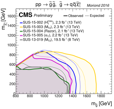
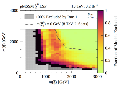
Often, searches are interpreted in terms of ‘simplified models’: for instance, one studies gluino pair production, then assumes that each decays into 2 jets and missing transverse momentum: see Fig. 15. However, current bounds based on simplified models [7] often give much stronger bounds than in a more general MSSM set-up [8]. This is because simplified models tend to only assume a single decay mode of one sparticle (or a few decay modes of particular sparticles), whereas in full models there can be literally thousands of active decay chains, diluting the signal between many different search channels such that no one shows an excess. There are also cases of somewhat ‘compressed spectra’: when sparticles in decay chains are similar in mass, energy-momentum conservation means that they tend to produce fairly soft SM particles, which often fail analysis cuts. Because they are not dependent on the many MSSM parameters, simplified searches are very convenient for searches, being less model dependent. However, exclusion limits from simplified models are not easy to interpret in more realistic models, and tend to be far too restrictive unless one interprets them with care. In Fig. 15, we see this in action: for massless neutralinos, gluinos up to 1750 GeV are ruled out in the simplified model, whereas in a (more realistic) phenomenological MSSM approximation, we see that gluinos of 800 GeV are still allowed for some points.

3 Extra Dimensions

For a review of extra dimensions and their phenomenology, see Ref. [10]. As mentioned above, extra dimensions correspond to an expansion of the Poincaré symmetry: there are additional generators associated with translation invariance in each extra spatial dimension. Superstring theory also requires them in addition to supersymmetry for internal consistency, but any theory incorporating them must explain why we only observe 3+1 (i.e.three space-like and one time-like). There are a couple of possibilities to ‘hide’ the extra dimensions from our perception:

• We are stuck on a brane: meaning that the bulk of space-time has more than 3+1 dimensions, but SM fields are stuck on a 3+1 dimensional hypersurface: a ‘brane’. Gravity travels wherever space-time is, so that it must feel the effect of the additional dimensions. That’s because gravity is a described by a quantum fluctuation of the metric, and the bulk metric is defined in the bulk space-time.

• The extra dimensions are curled up on themselves: each point in our 3+1 dimensional space time has a circle, or some other compact manifold, where one can travel – albeit periodically – in the extra dimensions, which are in an orthogonal direction to all of the other dimensions. If such manifolds are not too large (less than a millimeter, certainly), then current experimental bounds upon gravitational forces acting at relatively small distances may still not rule the model out.

Figure 16: Picture of different extra-dimensional set-ups: the brane (on the left), where in string theory SM states appear as open strings whose ends end upon the brane but gravitons appear as close string states in the bulk, or compactification (on the right), in this example we have taken the example of a circle $S^{1}$ times ordinary 4-dimensional Minkowski space $M^{4}$.

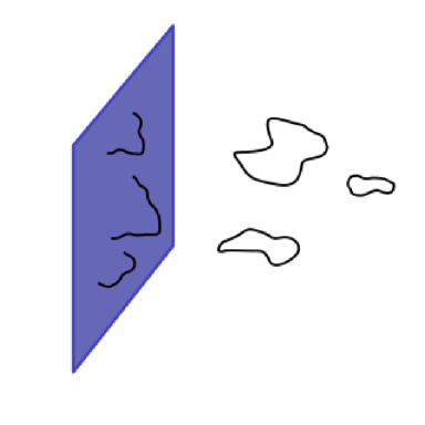
We illustrate the two cases in Fig. 16. In the figure, we have taken the example of string theory to illustrate the brane case, but it is essentially valid in the field theory limit as well: SM fields may be confined to a hypersurface of the bulk space-time, whereas gravity travels everywhere.

3.1 Compactification and a Scalar Field in 5 Dimensions

Taking compactified extra dimensions as an example, consider a massless five dimensional (5D) scalar field (i.e. a scalar field living in a 5-dimensional bulk space-time) $\varphi(x^{M}),M=0,1,\ldots,4$ with action

$${{\cal S}_{5\textrm{D}}=\int d^{5}x\partial^{M}\varphi\,\partial_{M}\varphi.}$$ (53)

We single the extra dimension out by calling it $x^{4}=y$. $y$ defines a circle of radius ${r}$ with $y\equiv y+2\pi r$. Our space time is now $\mathbb{M}_{4}\times S^{1}$. Periodicity in the $y$ direction implies that we may perform a discrete Fourier expansion

$${\varphi(x^{\mu},y)=\sum^{\infty}_{n=-\infty}\varphi_{n}(x^{\mu})\,\exp\left(\frac{iny}{r}\right).}$$ (54)

Notice that the Fourier coefficients are functions of the standard 4D coordinates and therefore are (an infinite number of) 4D scalar fields. The equations of motion for the Fourier modes are the (in general massive) Klein-Gordon wave equations

$${\partial^{M}\partial_{M}\varphi=0\Rightarrow\sum^{\infty}_{n=-\infty}\left(\partial^{\mu}\partial_{\mu}-\frac{n^{2}}{r^{2}}\right)\,\varphi_{n}(x^{\mu})\,\exp\left(\frac{iny}{r}\right)=0}$$

$$\Longrightarrow\framebox{{$\displaystyle\Bigl{.}\Bigr{.}\partial^{\mu}\partial_{\mu}\varphi_{n}(x^{\mu})-\frac{n^{2}}{r^{2}}\;\varphi_{n}(x^{\mu})=0.$} }$$ (55)

These are then an infinite number of Klein Gordon equations for massive 4D fields. This means that each Fourier mode $\varphi_{n}$ is a 4D particle with mass $m_{n}^{2}=\frac{n^{2}}{r^{2}}$. Only the zero mode ($n=0$) is massless. One can visualise the states as an infinite tower of massive states (with increasing mass proportional to $n$). This is called a Kaluza Klein tower and the massive states ($n\neq 0$) are called Kaluza Klein-states or momentum states, since they come from the momentum in the extra dimension:

Figure 17: The Kaluza Klein tower of massive states due to an extra $S^{1}$ dimension. Masses $m_{n}=|n|/r$ grow linearly with the fifth dimension’s wave number $n\in\mathbb{Z}$.

In order to obtain the effective action in 4D for all these particles, let us plug the mode expansion of $\varphi$ Eq. 54 into the original 5D action Eq. 53:

$${\cal S}_{5\textrm{D}} = \int d^{4}x\int dy\sum^{\infty}_{n=-\infty}\left({\partial^{\mu}\varphi_{n}(x^{\mu})\,\partial_{\mu}\varphi_{n}(x^{\mu})^{*}}-\frac{n^{2}}{r^{2}}|\varphi_{n}|^{2}\right)$$

$$= 2\,\pi\,r\int d^{4}x\bigl{(}{\partial^{\mu}\varphi_{0}(x^{\mu})\,\partial_{\mu}\varphi_{0}(x^{\mu})^{*}+\ldots}\bigr{)}={2\pi r{\cal S}_{4\textrm{D}}}+\ldots$$

This means that the 5D action reduces to one 4D action for a massless scalar field plus an infinite sum of massive scalar actions in 4D. If we are only interested in energies smaller than the $\frac{1}{r}$ scale, we may concentrate only on the action of the massless mode.

3.2 Compactification of a Vector Field in 5 Dimensions

Vector fields are decomposed in a completely analogous way: $\{A_{M}\}=\{A_{\mu},A_{4}=\phi\}$. Consider the action

$${\cal S}_{5\textrm{D}}=\int d^{5}x\frac{1}{g_{5\textrm{D}}^{2}}\;F_{MN}\,F^{MN}$$ (56)

with a field strength

$$F_{MN}=\partial_{M}A_{N}-\partial_{N}A_{M}$$ (57)

implying

$$\partial^{M}\partial_{M}A_{N}-\partial^{M}\partial_{N}A_{M}=0.$$ (58)

If we now choose a gauge, e.g. the transverse gauge:

$$\partial^{M}A_{M}=0,A_{0}=0\Rightarrow\partial^{M}\partial_{M}A_{N}=0,$$ (59)

then this obviously becomes equivalent to the scalar field case (for each component $A_{M}$) indicating an infinite tower of massive states for each massless state in 5D. In order to find the 4D effective action we once again plug this into the 5D action:

$${\cal S}_{5\textrm{D}} \mapsto {\cal S}_{4\textrm{D}}$$

$$= \int d^{4}x\left(\frac{2\pi r}{g_{5\textrm{D}}^{2}}\;F_{(0)}\,^{\mu\nu}\;F_{(0)\mu\nu}+\frac{2\pi r}{g_{5\textrm{D}}^{2}}\;\partial_{\mu}\rho_{0}\,\partial^{\mu}\rho_{0}+\ldots\right).$$

Therefore we end up with a 4D theory of a massless gauge particle $F^{\mu\nu}_{(0)}$, a massless scalar $\rho_{0}$ from the massless Kaluza-Klein state of $\phi$ and infinite towers of massive vector and scalar fields. Notice that the gauge couplings of 4- and 5 dimensional actions (coefficients of $F_{MN}F^{MN}$ and $F_{\mu\nu}F^{\mu\nu}$) are related by

$${\frac{1}{g_{4}^{2}}=\frac{2\pi r}{g_{5}^{2}}}.$$ (60)

In $D$ space time dimensions, this generalises to

$${\frac{1}{g_{4}^{2}}=\frac{V_{D-4}}{g_{D}^{2}}}$$ (61)

where $V_{n}$ is the volume of the $n$ dimensional compact space (e.g. an $n$ sphere of radius $r$).

3.2.1 The electric (and gravitational) potential

We apply Gauss’ law for the electric field $\vec{E}$ and the potential $\Phi$ of a point charge $Q$:

$$\oint\limits_{S^{2}}\vec{E}\cdot d\vec{S} = Q\Rightarrow\|\vec{E}\|\ \propto\frac{1}{R^{2}},\Phi\propto\frac{1}{R}:\ 4D$$

$$\oint\limits_{S^{3}}\vec{E}\cdot d\vec{S} = Q\Rightarrow\|\vec{E}\|\ \propto\frac{1}{R^{3}},\Phi\propto\frac{1}{R^{2}}:\ 5D$$

Thus, the apparent behaviour of the force depends upon whether we are sensitive to the extra dimension or not: if we test the force at distances smaller than its size (i.e. at energies high enough to probe such small distance scales), it falls off as $1/R^{3}$: the field lines have an extra dimension to travel in. If we test the force at larger distances than the size of the extra dimension, we obtain the usual $1/R^{2}$ law.

In $D$ space time dimensions

$$\|\vec{E}\|\propto\frac{1}{R^{D-2}},\Phi\propto\frac{1}{R^{D-3}}.$$ (62)

If one dimension is compactified (radius $r$) like in $\mathbb{M}_{4}\times S^{1}$, then we have two limits

$$\|\vec{E}\|\propto\left\{\begin{array}[]{ll}\displaystyle\frac{1}{R^{3}}&:R<r\\ \displaystyle\frac{1}{R^{2}}&:R\gg r\end{array}\right..$$ (63)

Analogous arguments hold for gravitational fields and their potentials, but we shall not detail them here, preferring instead to sketch the resulting field content.

3.2.2 Sketch of Compactified Gravitation

The spin 2$\hbar$ graviton $G_{MN}$ becomes the 4D graviton $g_{\mu\nu}$, some gravivectors $G_{\mu n}$ and some graviscalars $G_{mn}$ (where $m,n=4,\ldots,D-1$), along with their infinite Kaluza-Klein towers. The Planck mass squared ${M_{Pl}^{2}=M_{D}^{D-2}V_{D-4}\sim M_{D}^{D-2}r^{D-4}}$ is a derived quantity. Fixing $D$, we can fix $M_{D}$ and $r$ to get the correct result for $M_{Pl}\sim 10^{19}$ GeV. So far, we require $M_{D}>1$ TeV and $r<10^{-16}$cm from Standard Model measurements since no significant confirmed signature of extra dimensions has been seen at the time of writing.

3.3 Brane Worlds

Figure 18: Force field lines feel the effect of the extra dimensions. Here we show a 3+1 dimensional brane, where gravity spreads into the extra dimension and feels its effect.

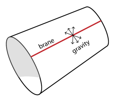
In the brane world scenario, we are trapped on a 3+1 surface in a $D+1$ dimensional bulk space-time (see Fig. 18). There are two cases here: large extra dimensions and warped space-times. Since gravity itself is so weak, the constraints on brane world scenarios are quite weak: the extra dimension is constrained to be of a size $r<0.1$ mm or so, potentially much larger than the $10^{-16}$ cm of the Standard Model, hence the name large extra dimensions.

3.3.1 Large extra dimensions

There is the possibility to try to solve the hierarchy problem with the large extra dimensions scenario if we put $M_{D}\sim 1$ TeV. The idea is that this is the fundamental scale: there is no high scale associated with $M_{Pl}$ fundamentally - it is an illusion caused by the presence of the extra dimensions. In 5D for example, $M_{Pl^{2}}=M_{D}^{D-2}V_{D-4}\Rightarrow r\sim 10^{8}$ km, clearly ruled out by observations. Already in 6D though, $r=0.1$ mm - consistent with experiments that measure the gravitational force on small distance scales. This rephrases the hierarchy problem to the question “why are the extra dimensions so large compared with $10^{-16}$ cm?”

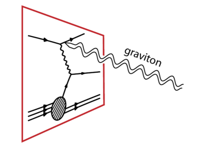
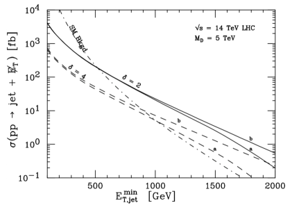
Graviton phenomenology: each Kaluza-Klein mode couples weakly $\propto 1/M_{Pl}$, but there are so many modes that after summing over them, you end up with $1/M_{D}$ suppression only! One can approximate them by a continuum of modes with a cut-off. The graviton tower propagates into the bulk and takes away missing momentum leading to a $pp\rightarrow j+\vec{p}_{\mathrm{T}}^{\mathrm{miss}}$ signature (for example) by the process shown in Fig. 19.

Figure 19: Example production of $\vec{p}_{\mathrm{T}}^{\mathrm{miss}}$ at a 14 TeV LHC through production of a Kaluza-Klein tower of graviton states that propagate off into the bulk. The left-hand panel shows a heuristic picture: the red hypersurface representing the brane, and the graviton tower being emitted into the bulk. In the right-hand panel, it is shown how the cross-section varies with the transverse momentum of the jet ($E^{min}_{T,jet}$) for the SM background, and the case of $d$ extra dimensions. The lines a (b) are constructed by integrating the cross-section over $\hat{s}<M_{D}^{2}$ (all $\hat{s}$), respectively. Both the diagram and the plot are from Ref. [11].

3.3.2 Warped (or ‘Randall-Sundrum’ space-times

Warped space-times are where the metric exponentially warps along the extra dimension $y$:

$${ds^{2}=e^{-|ky|}\eta_{\mu\nu}dx^{\mu}dx^{\nu}+dy^{2}.}$$ (64)

Figure 20: Picture of the Randall-Sundrum I set-up. On the left-hand side at $y=0$ we have the Planck brane, which is warped down to the weak brane at the right hand side ($y=\pi R$). The idea is that the Higgs boson (and some other fields) are localised on the weak brane.

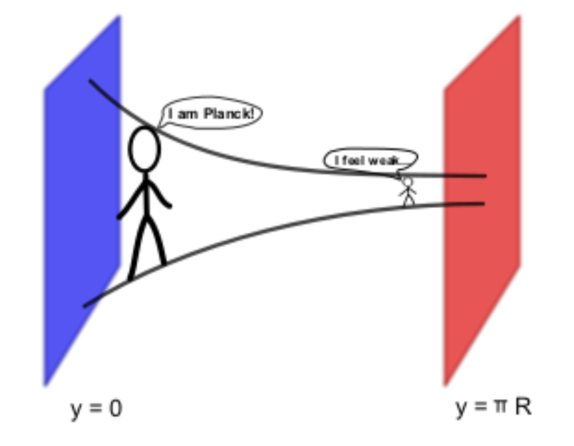
The metric changes from $y=0$ to $y=\pi r$ via $\eta_{\mu\nu}\mapsto e^{-k\pi r}\eta_{\mu\nu}$. Here, we set $M_{D}=M_{Pl}$, but this gets warped down to the weak brane:

$$\Lambda_{\pi}\sim M_{Pl}e^{-k\pi r}\sim\mathcal{O}(\textrm{TeV}),$$ (65)

if $r\sim 10/k$. Here, $k$ is of order $M_{Pl}$ and so we have a small extra dimension, but the warping explains the smallness of the weak scale. Note that we still have to stabilise the separation between the branes, which can involve extra tuning unless extra structure is added to the model.

The interaction Lagrangian is

$${{\mathcal{L}}_{I}=-G^{\mu\nu}T_{\mu\nu}/\Lambda_{\pi}},$$ (66)

where $T_{\mu\nu}$ is the stress energy tensor, containing products of the other Standard Model fields. $\Lambda_{\pi}\sim{\mathcal{O}}(\textrm{TeV}),$ so the interaction leads to electroweak-strength cross sections, not gravitationally suppressed ones. Thus, the LHC can produce the resonance: one will tend to produce the lightest one most often, as it is less suppressed by parton distribution functions. The ratios of masses of higher modes are given by zeros of Bessell functions, so they are not as regular as they are in large extra dimensions.

Randall-Sundrum phenomenology: one looks for the TeV scale first resonances, which are weakly coupled to Standard Model states. If only gravity travels in the extra dimensions, then the resonance is the ‘Randall-Sundrum graviton’: it has universal coupling to all particles via Eq. 66 and so it can decay into $q\bar{q}$, $WW$, $ZZ$, $\gamma\gamma$, $gg$, $l^{+}l^{-}$ or $h^{0}h^{0}$ with branching ratios that are of a similar order of magnitude to each other.

Figure 21: Production of an RS graviton and subsequent decay into $e^{+}e^{-}$: both figures are taken from Ref. [12]. On the right-hand side, the angular distribution of the electron with respect to the beam line in the rest-frame ($\theta^{*}$) of $G_{\mu\nu}$ is shown for a 1.5 TeV graviton. The different shaded colours show the contribution from $q\bar{q}$ collisions, from $gg$ and from other SM processes. This is contrasted against a straw-man spin 1$\hbar$ distribution in the green line. The typical expected size of statistical uncertainties resulting from 100 fb^-1 of integrated luminosity at a 14 TeV LHC is shown on the points. This would be enough to discriminate against the spin 1$\hbar$ hypothesis, which is much more forward than the spin 2$\hbar$ hypothesis.

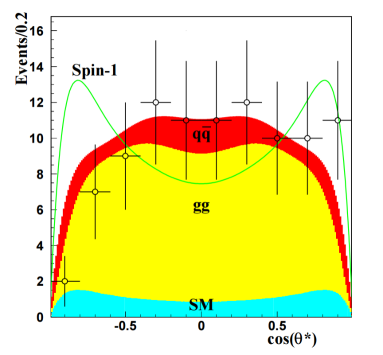
Flavour considerations imply that this isn’t the end of the story: one requires additional flavour structure, otherwise the model violates flavour bounds from experiment. One common way of adding flavour structure is to allow the other particles into the bulk, but have different profiles of fermions in the bulk, leading to different overlaps with the weak brane, where the Higgs field is localised (the overlap would be proportional to the particle in question’s Yukawa coupling). In this case, one could look for the first Kaluza Klein modes of gauge bosons and fermions, too.

Kaluza Klein modes that have masses that are heavier than the centre of mass energy of the beams may also be looked for via their virtual effects. Searching for particles that mediate interactions that are occurring at collisions with less energy than their mass has been historically very important (particularly in terms of the weak interactions which were indirectly observed before the discovery of the $W^{\pm}$ and $Z^{0}$ bosons). Such a kinematic situation can be approximated by effective field theories, which in turn reduces model dependence. We now sketch effective field theories, along with caveats pertinent to their use.

4 Effective Field Theories

At low momenta $p^{\mu}$, we can model the effects of particles with a much heavier mass $M^{2}\gg p^{2}$ and a small width $\Gamma\ll M$ with effective field theory. This squeezes a propagator down to a point:

$$\text{lim}_{p^{2}/M^{2}\rightarrow 0,\Gamma/M\rightarrow 0}{\frac{1}{p^{2}-M^{2}+iM\Gamma}\approx-\frac{1}{M^{2}},}$$ (67)

in a fairly model independent way. Thus, for example $W$ boson couplings between like

$${{\mathcal{L}}=-\frac{g}{2\sqrt{2}}\bar{e}\gamma^{\rho}(1-\gamma_{5})W_{\rho}{\nu_{e}}-\frac{g}{2\sqrt{2}}\bar{\nu}_{\mu}\gamma^{\rho}(1-\gamma_{5})W_{\rho}\mu}$$ (68)

becomes

$${{\mathcal{L}}\approx-\frac{G_{F}}{\sqrt{2}}\left(\bar{e}\gamma^{\rho}(1-\gamma_{5}){\nu_{e}}\right)\left(\bar{\nu}_{\mu}\gamma^{\rho}(1-\gamma_{5})\mu\right),}$$ (69)

where $G_{F}=\sqrt{2}g^{2}/(8M_{W}^{2})$. One has to be careful at the LHC with the range of validity of the effective field theory, however, because the LHC has a large centre of mass energy. If some of the collisions have $p^{2}\geq M^{2}$, then for those collisions the effective field theory is a bad approximation: there, one becomes sensitive to the full structure of the propagator. Effective field theory methods can be useful for parameterising searches for new physics at low momentum: these four-fermion operators are often called contact operators, e.g. for some fermionic dark matter particle $\chi$,

$${\mathcal{L}}=\frac{\lambda^{2}}{M^{2}}(\bar{q}\gamma^{\mu}q)(\chi\gamma_{\mu}\chi)$$ (70)

for some coupling strength $\lambda$ [18]. However, for dark matter production at the LHC (e.g. in the monojet channel), the energies are often higher than the messenger mass and so a more precise (simplified?) model is needed [19]. Such a move to more specified models increases model dependence, but may be necessary if one requires a large régime of validity for one’s description of high energy collisions.

5 Conclusion

At the time of writing, 13 TeV collisions at the LHC have yet to yield direct, unambiguous and confirmed discoveries of new physics. In some channels, around 36 fb^-1 of integrated luminosity has been analysed in each general purpose experiment. However, there is plenty of room for new physics to be hiding: in more data or in other analyses. I personally and perhaps naively expect some signal to show up in the first 100 fb^-1 of Run II data. Certainly it seems unlikely that if there are no excesses at all in that amount of data (in some channel), there is unlikely to be a $5\sigma$ discovery at Run II in the same channel. If CERN increases the beam energy, for example from 13 TeV to 14 TeV, the search sensitivity gains a sudden boost, and indeed this will be interesting in Run III or beyond. There is a plan (the ‘high-energy’ LHC, or HE-LHC) to increase the beam energy to around 27 TeV with new magnets. This would lead to a large increase in sensitivity.

Figure 22: Example Feynman diagram contributing to $B$ meson decays that form the variable $R_{K}$.

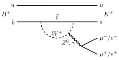
On the other hand, there are several interesting excesses in $B$ physics measurements as compared to SM measurements, which we have not explicitly discussed in these Beyond the Standard Model lectures. Probably the theoretically cleanest of these are those of $R_{K^{(*)}}$ as shown in Table 1.

	$q^{2}$/GeV2	SM	LHCb 3 fb	$\sigma$
$R_{K}$	$[1,6]$	$1.00\pm 0.01$	${\bf 0.745}^{+0.090}_{-0.074}$	2.6
$R_{K^{\ast}}$	$[0.045,1.1]$	$0.91\pm 0.03$	${\bf 0.66}^{+0.11}_{-0.07}$	2.2
$R_{K^{\ast}}$	$[1.1,6]$	$1.00\pm 0.01$	${\bf 0.69}^{+0.11}_{-0.07}$	2.5

Table 1: Predictions and measurements of $R_{K^{(*)}}\equiv\frac{BR(B^{\pm}\rightarrow{K^{(*)}}^{\pm}\mu^{+}\mu^{-})}{BR(B^{\pm}\rightarrow{K^{(*)}}^{\pm}e^{+}e^{-})}$ [13] in different bins of momentum transfer squared. The uncertainty on the SM prediction includes estimated theoretical uncertainties.

from the LHCb experiment [13, 14]. Large theoretical uncertainties associated with mesonic physics cancel well in such a ratio, particularly when one is probing final states involving leptons. In the SM, $R_{K}$ is a firm prediction from diagrams like Fig. 22, and so the measurements in Table 1 indicate non-SM lepton flavour non-universality at the 4$\sigma$ level. In fact, a fit to this and other data indicates that a new physics effective field theory operator on top of the SM

$${\mathcal{L}}=C_{9}^{(\mu)}(\bar{s}_{L}\gamma^{\mu}b_{L})(\bar{\mu}_{L}\gamma_{\mu}\mu_{L})+\ldots$$ (71)

is preferred to be non-zero at the 4.3$\sigma$ level [15, 16, 17]. A BSM operator proportional to $(\bar{s}_{L}\gamma^{\mu}b_{L})(\bar{\mu}\gamma_{\mu}\mu)$ (i.e. a vector-like coupling to muons, rather than a left-handed coupling to them) also works approximately as well. At the tree-level, these operators can be caused by a couple of different BSM particles: leptoquarks or flavourful $Z^{\prime}$s, as depicted in Fig. 23.

Figure 23: Feynman diagrams showing different possibilities for BSM particles of mass $M\gg m_{B}$ which lead to the effective operator in Eq. 71 at tree-level. The additional particles lead to a change in $C_{9}^{(\mu)}$ proportional to $-\lambda_{1}\lambda_{2}/M^{2}$, where $\lambda_{1,2}$ are dimensionless couplings of the respective particles. This combination of couplings and masses are then fixed to predict the central value of the experimental measurements of $B-$data.

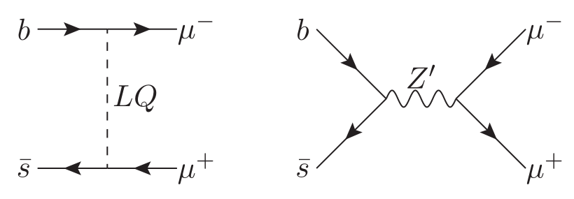
The leptoquark can either be a scalar triplet $S_{3}$ of $SU(2)_{L}$ or a vector particle: either an $SU(2)_{L}$ triplet, or singlet. Leptoquarks couple (by definition) to a lepton and a quark: in order to preserve QCD they must therefore be coloured. Hadron collider and other searches then focus on pair production of them, e.g. by the process $gg\rightarrow S_{3}{\bar{S}}_{3}\rightarrow(\mu^{+}b)\ (\mu^{-}\bar{s})$, where the bracketed particles should form a resonance and have a bump in their invariant mass spectra. In the case of $Z^{\prime}$ particles, the diagram in Fig. 23 leads to resonant production of $Z^{\prime}$, since the initial $b$ quark can be obtained from an initial proton from a gluon splitting into a $b\bar{b}$ pair.

Figure 24: 100 TeV Future Circular Collider (FCC) reach for flavourful $Z^{\prime}$s (left panel) and leptoquarks that explain the $R_{K^{(*)}}$ data (right panel). The red area in the left-hand plot is excluded by measurements of $B_{s}-\bar{B}_{s}$ mixing, whereas the blue area is the 95$\%$ confidence level (CL) projected sensitivity. The grey area shows wide $Z^{\prime}$ particles, where perturbativity is being lost. In the right-hand panel, the region above each curve is covered at 95$\%$, whereas the production cross-section is shown by the dotted curve. Figures from Ref. [20].

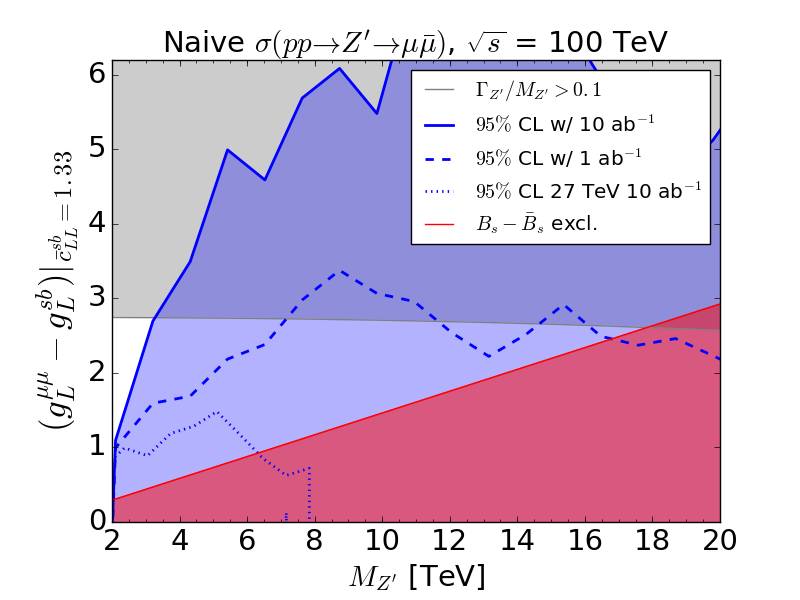
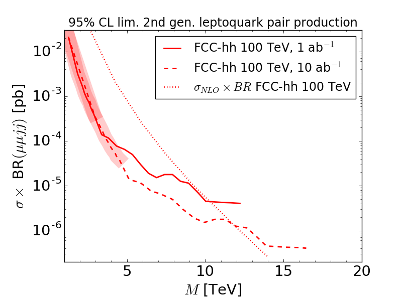
We show the projected sensitivity of a future 100 TeV $pp$ collider to such particles that explain the errant $B$ decays in Fig. 24. In the left-hand plot, we see that a 27 TeV energy upgraded LHC option covers a small portion of the $Z^{\prime}$ parameter space, whereas the 100 TeV option can essentially cover all of the allowed perturbative parameter space. In the right-hand plot, we deduce that leptoquarks with a mass up to 12 TeV can be covered by a FCC pair-production search. Leptoquarks up to 40 TeV in mass can explain the $B-$data whilst still satisfying other constraints. However, since it is the particular combination $\lambda_{1}\lambda_{2}/M^{2}$ is fixed by the $B-$data, $M$ and $\lambda_{1,2}$ can all be much smaller. Searches at the LHC, HL-LHC and HE-LHC are therefore of high priority (this also goes for $Z^{\prime}$s). LHCb is expected to announce further measurements of the quantities in Table 1 in 2019, with a roughly similar-size and independent data set.

We close with a quote from William Blake from The Marriage of Heaven and Hell:

“The road of excess leads to the palace of wisdom”.

References

- [1] F. Quevedo, S. Krippendorf and O. Schlotterer, arXiv:1011.1491 [hep-th].
- [2] K.A.Olive et al (Particle Data Group), Chin. Phys. C38 (2014) 090001.
- [3] S. P. Martin, Adv. Ser. Direct. High Energy Phys. 21 (2010) 1 [Adv. Ser. Direct. High Energy Phys. 18 (1998) 1] doi:10.1142/9789812839657_0001, 10.1142/9789814307505_0001 [hep-ph/9709356].
- [4] B. C. Allanach, Comput. Phys. Commun. 143 (2002) 305 doi:10.1016/S0010-4655(01)00460-X [hep-ph/0104145].
- [5] B. C. Allanach, S. Grab and H. E. Haber, JHEP 1101 (2011) 138 Erratum: [JHEP 1107 (2011) 087] Erratum: [JHEP 1109 (2011) 027] doi:10.1007/JHEP07(2011)087, 10.1007/JHEP09(2011)027, 10.1007/JHEP01(2011)138 [arXiv:1010.4261 [hep-ph]].
- [6] C. Young (on behalf of ATLAS and CMS Collaborations), talk at Electroweak Session of Moriond 2016 conference, La Thuile, Italy.
- [7] D. Alves et al. [LHC New Physics Working Group Collaboration], J. Phys. G 39 (2012) 105005 doi:10.1088/0954-3899/39/10/105005 [arXiv:1105.2838 [hep-ph]].
- [8] G. Aad et al. [ATLAS Collaboration], JHEP 1510 (2015) 134 doi:10.1007/JHEP10(2015)134 [arXiv:1508.06608 [hep-ex]].
- [9] A. Barr and J. Liu, arXiv:1605.09502 [hep-ph].
- [10] S. Raychaydhuri and K. Sridhar, Cambridge Monographs on Mathematical Physics, Cambridge University Press (2016), ISBN 9780521768566.
- [11] G. F. Giudice, R. Rattazzi and J. D. Wells, Nucl. Phys. B 544 (1999) 3 doi:10.1016/S0550-3213(99)00044-9 [hep-ph/9811291].
- [12] B. C. Allanach, K. Odagiri, M. A. Parker and B. R. Webber, JHEP 0009 (2000) 019 doi:10.1088/1126-6708/2000/09/019 [hep-ph/0006114].
- [13] R. Aaij et al. [LHCb Collaboration], Phys. Rev. Lett. 113 (2014) 151601 doi:10.1103/PhysRevLett.113.151601 [arXiv:1406.6482 [hep-ex]].
- [14] R. Aaij et al. [LHCb Collaboration], JHEP 08 (2017) 055 [arXiv:1705.05802 [hep-ex]]
- [15] S. Descotes-Genon, J. Matias and J. Virto, Phys. Rev. D 88 (2013) 074002 doi:10.1103/PhysRevD.88.074002 [arXiv:1307.5683 [hep-ph]].
- [16] W. Altmannshofer and D. M. Straub, Eur. Phys. J. C 75 (2015) no.8, 382 doi:10.1140/epjc/s10052-015-3602-7 [arXiv:1411.3161 [hep-ph]].
- [17] S. Descotes-Genon, L. Hofer, J. Matias and J. Virto, JHEP 1606 (2016) 092 doi:10.1007/JHEP06(2016)092 [arXiv:1510.04239 [hep-ph]].
- [18] J. Goodman, M. Ibe, A. Rajaraman, W. Shepherd, T. M. P. Tait and H. B. Yu, Phys. Rev. D 82 (2010) 116010 doi:10.1103/PhysRevD.82.116010 [arXiv:1008.1783 [hep-ph]].
- [19] J. Abdallah et al., Phys. Dark Univ. 9-10 (2015) 8 doi:10.1016/j.dark.2015.08.001 [arXiv:1506.03116 [hep-ph]].
- [20] B.C. Allanach, B. Gripaios and T. You, JHEP 1803 (2018) 021, [arXiv:1710.06363 [hep-ph]].