Doubly Stochastic Neighbor Embedding on Spheres

Abstract

Stochastic Neighbor Embedding (SNE) methods minimize the divergence between the similarity matrix of a high-dimensional data set and its counterpart from a low-dimensional embedding, leading to widely applied tools for data visualization. Despite their popularity, the current SNE methods experience a crowding problem when the data include highly imbalanced similarities. This implies that the data points with higher total similarity tend to get crowded around the display center. To solve this problem, we introduce a fast normalization method and normalize the similarity matrix to be doubly stochastic such that all the data points have equal total similarities. Furthermore, we show empirically and theoretically that the doubly stochasticity constraint often leads to embeddings which are approximately spherical. This suggests replacing a flat space with spheres as the embedding space. The spherical embedding eliminates the discrepancy between the center and the periphery in visualization, which efficiently resolves the crowding problem. We compared the proposed method (DOSNES) with the state-of-the-art SNE method on three real-world datasets and the results clearly indicate that our method is more favorable in terms of visualization quality. DOSNES is freely available at http://yaolubrain.github.io/dosnes/.

1 Introduction

Information visualization by dimensionality reduction facilitates a viewer to quickly digest information in massive data. It is therefore increasingly applied as a critical component in scientific research, digital libraries, data mining, financial data analysis, market studies, manufacturing production control and drug discovery, etc. Numerous dimensionality reduction methods have been introduced, ranging from linear methods such as Principal Component Analysis to nonlinear methods such as Multidimensional Scaling (MDS), (MDS; Torgerson, 1952), Isomap (Tenenbaum et al., 2000), Locally Linear Embedding (Roweis and Saul, 2000), Curvilinear Component Analysis (Demartines and Hérault, 1997), Laplacian Eigenmaps (Belkin and Niyogi, 2001), and Gaussian Process Latent Variable Models (Lawrence, 2004). A survey on nonlinear dimensionality reduction has been given by van der Maaten et al. (2009). Aspects in Multidimensional Scaling are discussed by Buja et al. (2008).

Recently, Stochastic Neighbor Embedding (SNE) and its variants (Hinton and Roweis, 2002; van der Maaten and Hinton, 2008; van der Maaten, 2014; Yang et al., 2014; Sun et al., 2015; Tang et al., 2016) have achieved remarkable progress in data visualization, especially for displaying clusters in data. An SNE method takes as input the pairwise similarities between data points in the high-dimensional space and tries to preserve the similarities in a low-dimensional space by minimizing the Kullback-Leibler divergence between the input and output similarity matrices.

The input to SNE is a similarity matrix or the affinity matrix of a weighted graph. When the node degrees of the graph are highly imbalanced, SNE tends to place the high-degree nodes in the center and the low-degree ones in the periphery, regardless of the intrinsic similarities between the nodes. Therefore, SNE often experiences the “crowding-in-the-center” problem for highly imbalanced affinity graphs.

We propose two techniques to overcome the above-mentioned drawback. First, we impose a doubly stochasticity constraint on the input similarity matrix. Two-way normalization has been shown to improve spectral clustering (Zass and Shashua, 2006) and here we verify that it is also beneficial for data visualization. Moreover, if the neighborhood graph is asymmetric, for example, $k$-Nearest-Neighbors ($k$NN) or entropy affinities (van der Maaten and Hinton, 2008; Vladymyrov and Carreira-Perpiñán, 2013), we provide an efficient method for converting it to a doubly stochastic matrix.

Second, we observe that the data points are often distributed approximately around a sphere if the input similarity matrix is doubly stochastic, and we provide a theoretical analysis of this phenomenon. Our analysis suggests replacing the two-dimensional Euclidean embedding space with spheres in the three-dimensional space. Since there is no global center or periphery on the sphere geometry, the visualization is then naturally free of “crowding-in-the-center” problem. Moreover, we present an efficient projection step for adapting an SNE method with the spherical constraint.

We tested the proposed method on several real-world datasets and compared it with the state-of-the-art SNE method, t-SNE (van der Maaten and Hinton, 2008). The new method is superior to t-SNE in resolving the crowding problem and in preserving intrinsic similarities.

In the next section we briefly review SNE methods. We then discuss doubly stochastic similarity matrix and spherical embedding in Sections 3 and 4, respectively. We present experimental results in Section 5 and conclusions in Section 6.

2 Stochastic Neighbor Embedding

Stochastic Neighbor Embedding (SNE; Hinton and Roweis, 2002) is a nonlinear dimensionality reduction method. Given a set of multivariate data points $\{x_{1},x_{2},\dots,x_{n}\}$, where $x_{i}\in\mathbb{R}^{D}$, their neighborhood is encoded in a square nonnegative matrix $P$, where $P_{ij}$ is the probability that $x_{j}$ is a neighbor of $x_{i}$. SNE finds a mapping $x_{i}\mapsto y_{i}\in\mathbb{R}^{d}$ for $i=1,\dots,n$ such that the neighborhoods are approximately preserved in the mapped space. Usually the mapping is defined such that $d=2$ or $3$, and $d<D$. If the neighborhood in the mapped space is encoded in $Q\in\mathbb{R}^{n\times n}$ such that $Q_{ij}$ is the probability that $y_{j}$ is a neighbor of $y_{i}$, the SNE task is to minimize the Kullback-Leibler divergence $\mathcal{D}_{\text{KL}}(P||Q)$ over $Y=\left[y_{1},y_{2},\dots,y_{n}\right]^{T}$.

Symmetric Stochastic Neighbor Embedding (s-SNE; van der Maaten and Hinton, 2008) is a variant of SNE. Given input similarity $p_{ij}\geq 0$, s-SNE minimizes Kullback-Leibler divergence between the matrix-wise normalized similarities $P_{ij}=p_{ij}/\sum_{ab}p_{ab}$ and $Q_{ij}=q_{ij}/\sum_{ab}q_{ab}$. The output similarity $q_{ij}$ is typically chosen to be proportional to a Gaussian distribution so that $q_{ij}=\exp\left(-\|y_{i}-y_{j}\|^{2}\right)$, or proportional to a Cauchy distribution so that $q_{ij}=(1+\|y_{i}-y_{j}\|^{2})^{-1}$. The Cauchy s-SNE method is also called t-Distributed Stochastic Neighbor Embedding (t-SNE; van der Maaten and Hinton, 2008). The optimization of s-SNE can be implemented with the gradients for Gaussian case: $\partial\mathcal{J}/\partial y_{i}=4\sum_{j}(P_{ij}-Q_{ij})(y_{i}-y_{j})$ and for Cauchy case $\partial\mathcal{J}/\partial y_{i}=4\sum_{j}(P_{ij}-Q_{ij})(y_{i}-y_{j})q_{ij}$. Here $4\sum_{j}P_{ij}(y_{i}-y_{j})$ or $4\sum_{j}P_{ij}(y_{i}-y_{j})q_{ij}$ can be interpreted as the attractive force for $y_{i}$, while $-4\sum_{j}Q_{ij}(y_{i}-y_{j})$ or $-4\sum_{j}Q_{ij}(y_{i}-y_{j})q_{ij}$ as the repulsive force.

3 Doubly Stochastic Similarity Matrix

The input to s-SNE, $P$, is a nonnegative and symmetric matrix and can be treated as the affinity matrix of an undirected weighted graph. If the degree (i.e. row sum or column sum of $P$) distribution of nodes is highly non-uniform, then the high-degree nodes will usually receive and emit more attractive force than the average nodes during the iterative learning. As a result, these nodes often glue together and form the center of display. On the other hand, the low-degree nodes tend to be placed in the periphery due to less attraction. This behavior is often undesired in visualization because it only reveals the data centrality but hinders the discovery of other useful patterns, and may be directly misleading when some high-degree nodes are actually disconnected in the underlying data.

To overcome the above drawback, we can normalize the graph affinity such that the nodes have the same degree. For undirected graphs, this can be implemented by replacing the unitary matrix-wise sum constraint $\sum_{ij}P_{ij}=1$ in s-SNE with the doubly stochasticity constraint, i.e. $\sum_{i}P_{ij}=\sum_{j}P_{ij}=1$.

Given a non-normalized matrix, we can apply Sinkhorn-Knopp (Sinkhorn and Knopp, 1967) or Zass-Shashua method (Zass and Shashua, 2006) to project it to the closest doubly stochastic matrix $P$. In this work we use the former because it can maintain the sparsity of in the similarity matrix, which is often needed for large-scale tasks. Given a non-normalized similarity matrix $S$, the Sinkhorn-Knopp method initializes $P=S$ and iterates the following update rules until $P$ has converged:

$$\text{for all }i,~{}~{}u_{i}\leftarrow\sum_{j}P_{ij},$$ (1)

$$\text{for all }i,j,~{}~{}P_{ij}\leftarrow P_{ij}u_{i}^{-1/2}u_{j}^{-1/2}.$$ (2)

Alternatively, the neighborhood information in high-dimensional space can be encoded in an asymmetric matrix $B\geq 0$ with $n$ rows, for example, the $k$NN graph or the entropy affinities (van der Maaten and Hinton, 2008; Vladymyrov and Carreira-Perpiñán, 2013). $B$ can also be a non-square dyadic data such as document-term or author-paper co-occurrence matrix. In these cases, we can apply the following steps to construct a doubly stochastic matrix: suppose $\sum_{k}B_{ik}>0$ for all $i$, we first calculate for all $i,k$,

$$A_{ik} \leftarrow\frac{B_{ik}}{\sum_{u}B_{iu}},$$ (3)

and then for all $i,j$

$$P_{ij} \leftarrow\sum_{k}\frac{A_{ik}A_{jk}}{\sum_{v}A_{vk}}.$$ (4)

It is easy to verify that by this construction $P$ is symmetric and doubly stochastic. The calculations of $A$ and $P$ are performed only once and are thus computationally much more efficient than Sinkhorn-Knopp method which needs iterative steps. Here the matrix $A_{ik}$ can be treated as the random walk probability from the $i$th row index to the $k$th column index and $P_{ij}$ is interpreted as the two-step random walk probability between two row indices $i$ and $j$ via any column index $k$ (with uniform prior over row indices). Besides computational considerations, the choice of which projection to use is also data-dependent.

4 Spherical Embedding of Doubly Stochastic Similarity Matrices

When the input similarity matrix is doubly stochastic, we find that s-SNE often embeds the data points around a sphere in the low-dimensional space. The phenomenon is illustrated in Figure 1, where we generated a 2000$\times$2000 similarity matrix with uniform distribution and visualize it by t-SNE. We can see from the left subfigure that the embedding is close to a ball. In contrast, if the matrix is doubly stochastically normalized (by using the Sinkhorn-Knopp method), the resulting embedded points approximately lie around a circle. The same phenomenon also holds for 3D visualizations.

Figure 1: t-SNE visualization of a random uniformly distributed matrix (left) and a random doubly stochastic matrix (right).

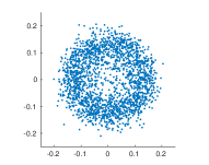
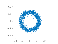
We provide a theoretical analysis of this phenomenon. If $P$ is doubly stochastic, then $Q$ is often approximately doubly stochastic (up to a constant factor) because it approximates $P$ by the KL-divergence. That is, $\sum_{j}Q_{ij}$ is approximately the same for all $i$. For example, in Figure 1 (right), $\sum_{j}Q_{ij}$ mainly distribute around a constant (with mean $0.0005$ and very small standard deviation $1.7\times 10^{-6}$). In this case, we show that $\sum_{j}\|y_{i}-y_{j}\|^{2}$ becomes approximately the same for all $i$, bounded by constants, in Proposition 4.1. Furthermore, we show that when $\sum_{j}\|y_{i}-y_{j}\|^{2}$ is exactly the same for all $i$, the embedded points must be on a sphere, in Proposition 4.2. The proofs of the propositions are provided in the supplemental document.

Proposition 4.1.

If $\sum_{j}q_{ij}=c$ for $i=1,\dots,n$ and $c>0$, then $L\leq\sum_{j}\|y_{i}-y_{j}\|^{2}\leq U$, where 1) for $q_{ij}=\exp(-\|y_{i}-y_{j}\|^{2})$, $L=n\ln\frac{n}{c}$ and $U=n\ln\frac{n}{c-nb}$, with $b=a+(1-a)m-m^{a}$, $m=\min_{j}\exp(-\|y_{i}-y_{j}\|^{2})$ and $a=\displaystyle\frac{\ln[\ln(1/m)/(1-m)]}{\ln(1/m)}$; 2) for $q_{ij}=(1+\|y_{i}-y_{j}\|^{2})^{-1}$, $L=\frac{n^{2}}{c}-n$ and $U=\frac{n^{2}}{c}-n+n(\sqrt{b}-1)^{2}$, with $b=1+\max_{j}\|y_{i}-y_{j}\|^{2}$.

Proposition 4.2.

If $\sum_{j}\|y_{i}-y_{j}\|^{2}=c$ for $i=1,\dots,n$, $c>0$ and $\sum_{i}y_{i}=0$, then $\|y_{1}\|^{2}=\|y_{2}\|^{2}=\dots=\|y_{n}\|^{2}$.

Since the embedding is often nearly spherical for doubly stochastic similarity matrices, it is more suitable to replace the 2D Euclidean embedding space with spheres in 3D space. The resulting layout can be encoded with $n\times 2+1$ numbers (two angles for each data point plus the common radius). Therefore the embedding is still intrinsically two-dimensional.

The spherical geometry itself brings other benefits for visualization. First, the embedding in the Euclidean space has a global center in the middle, while on spheres there is no such global center. Therefore a spherical visualization is free of the “crowding-in-the-center” problem. Every point on the sphere can be a local center, which provides fish-eye views for navigation and for examining patterns beyond centrality. Second, the attractive and repulsive forces can be transmitted in a cyclic manner, which helps in discovering macro patterns such inter-cluster similarities.

We thus formulate our learning objective as follows:

$$\mathop{{\symoperators minimize}}_{Y\in\mathbb{S}}~{} ~{}\mathcal{J}(Y)=\mathcal{D}_{\text{KL}}(P||Q),$$ (5)

where $\mathcal{J}(Y)$ is an SNE objective function with $P$ doubly stochastic, $Q$ defined in Section 2 and

$$\mathbb{S}=\left\{Y~{}\Big{|}~{}Y\in\mathbb{R}^{n\times 3};\|y_{1}\|=\dots=\|y_{n}\|;~{}\sum_{i}y_{i}=0\right\}.$$ (6)

We call the new method DOubly Stochastic Neighbor Embedding on Spheres (DOSNES). Note that $\mathbb{S}$ includes all centered spheres in the three-dimensional space, not only the unit sphere.

We employ a projection step after each SNE update step to enforce the sphere constraint. The DOSNES algorithm steps are summarized as follows:

1. Normalize $P$ to be doubly stochastic.

2. Repeat until convergence

   1. $\widetilde{Y}\leftarrow$OneStepUpdateSNE($P$, $Y$),

   2. $Y\leftarrow\arg\min_{Z\in\mathbb{S}}\|Z-\widetilde{Y}\|$.

The projection step 2b is performed by implicitly switching $\widetilde{Y}=[\tilde{y}_{1},\dots,\tilde{y}_{n}]^{T}$ to the spherical coordinate system, taking the mean radius, and switching back to Cartesian coordinates. This is implemented as: For $i=1,\dots,n$

$$\tilde{y}_{i} \leftarrow\tilde{y}_{i}-\frac{1}{n}\sum_{j}\tilde{y}_{j},$$ (7)

$$y_{i} \leftarrow\frac{\tilde{y}_{i}}{\|\tilde{y}_{i}\|}\cdot\left(\frac{1}{n}\sum_{j}\|\tilde{y}_{j}\|\right).$$ (8)

The iterations converge to a stationary point with suitable learning step sizes (see e.g., Iusem, 2003, Section 5).

We do not take gradient steps directly with respect to the latitude and longitude parameters, because such gradients give no information for learning the sphere radius and require expensive trigonometric functions.

5 Experiments

We developed a browser-based software for displaying and navigating the DOSNES results. The software and its demos can be found in the project website. In the paper we present the 2D projected views of the spheres.

We compare our proposed method DOSNES with two- and three-dimensional t-SNE as well as non-metric MDS in Euclidean embedding space (van der Maaten and Hinton, 2008) to verify the effectiveness of using doubly stochastic similarities and the sphere constraint.

The compared methods were tested on three real-world datasets from different domains:

1) NIPS: the proceedings of NIPS conferences (1987-2015) which contains 5,993 papers and their associated 6,621 authors. We used the largest connected component in the co-author graph with 5,300 papers and 5,422 authors. The (non-normalized) similarity matrix is from the co-author graph, i.e. $BB^{T}$ where $B$ is the author-paper co-occurrence matrix.

2) WorldTrade: trade network of metal manufactures among 80 countries in 1994. Each edge represents the total trade amount (imports and exports) between two countries.

3) MIREX: the dataset is from the the Third Music Information Retrieval Evaluation eXchange (MIREX 2007). It is a network of 3090 songs in 10 music genre classes. The weighted edges are human judgment on how similar two songs are.

MDS requires a distance matrix as input. Given a similarity matrix $S$, we first normalize $\widetilde{S}_{ij}=S_{ij}/\max(S)$. Treating $\widetilde{S}_{ij}^{\prime}s$ as cosine similarities, we obtain the cosine distances by $D_{ij}=1-\widetilde{S}_{ij}$. Next we calculate the shortest graph distances between all nodes and feed them to MDS.

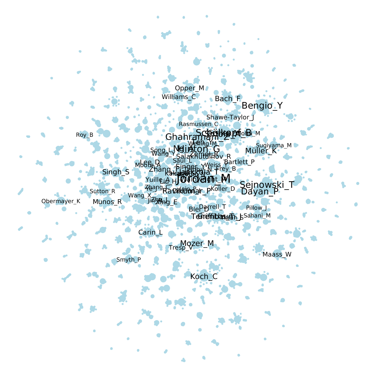
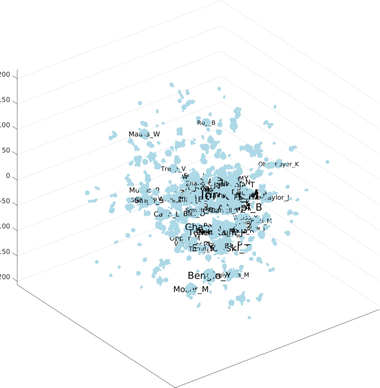
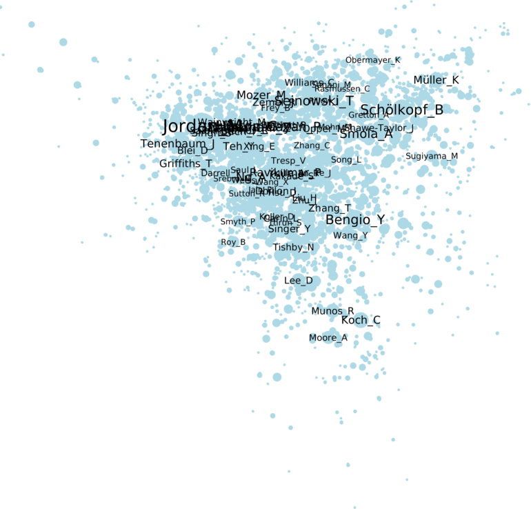
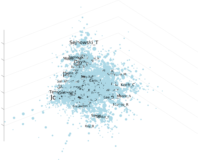
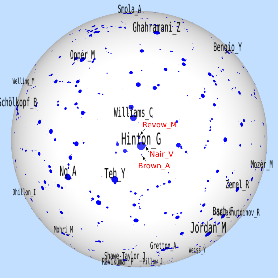
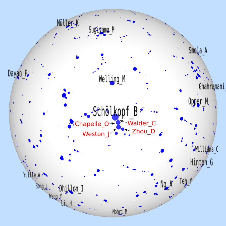
The NIPS co-author graph is visualized in Figure 2. The node degrees of the graph are highly uneven, where many authors have only one paper while the the most productive author has 93 papers. In Figure 2 (a) and (b), we can see both 2D and 3D t-SNE caused the most productive NIPS authors crowded in the center. This is undesirable because these authors actually do not often co-author NIPS papers. For example, Hinton_G has no co-authored paper with Schölkopf_B but they are very close in the t-SNE layout. A similar crowding problem is observed in the MDS visualizations. In Figure 2 (e) and (f), DOSNES resolves neatly the crowding problem, by normalizing the similarity matrix with our method in Section 3 and visualizing the authors with spherical layout. The productive NIPS authors are now more evenly distributed. For example, Hinton_G becomes more distant to Schölkopf_B. Meanwhile, retrieval around the most established authors reveals accurate co-authorship. For example, Revow_M, Nair_V and Brown_A are close to Hinton_G because all their NIPS papers are co-authored with Hinton_G. See our online demo for more details.

(a) t-SNE 2D

(b) t-SNE 3D

(c) MDS 2D

(d) MDS 3D

(e) DOSNES (viewpoint 1)

(f) DOSNES (viewpoint 2)

Figure 2: Visualizations of the NIPS dataset.

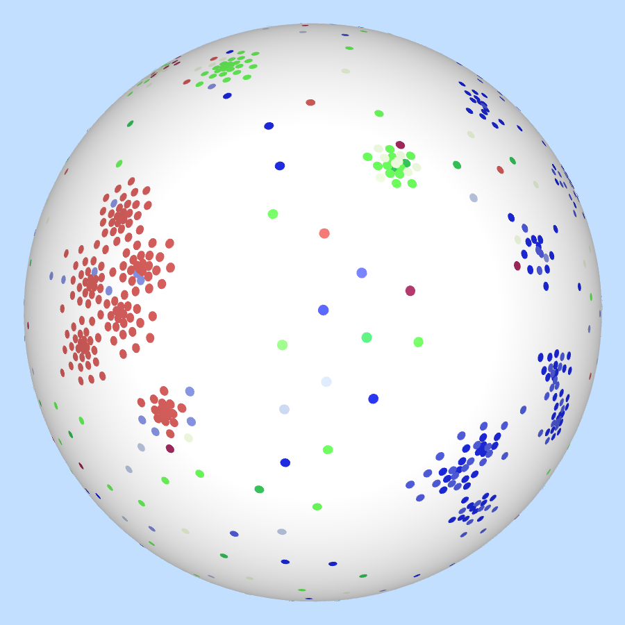
The visualizations of the WorldTrade graph are given in Figure 3. In this graph, some countries such as United States and Germany have more total trade amount than many others. In Figure 3 (a) to (d), we can see both 2D and 3D t-SNE, as well as the MDS visualizations, caused these countries crowded in the center. In contrast, DOSNES places the countries more evenly. In Figure 3 (e) and (f), we can see on the sphere many meaningful clusters (e.g., Europe and Asia) which well match the geography even though we did not use such information in the training. See our demo globe for other viewpoints.

(a) t-SNE 2D

(b) t-SNE 3D

(c) MDS 2D

(d) MDS 3D

(e) DOSNES (viewpoint 1)

(f) DOSNES (viewpoint 2)

Figure 3: Visualizations of the WorldTrade dataset.

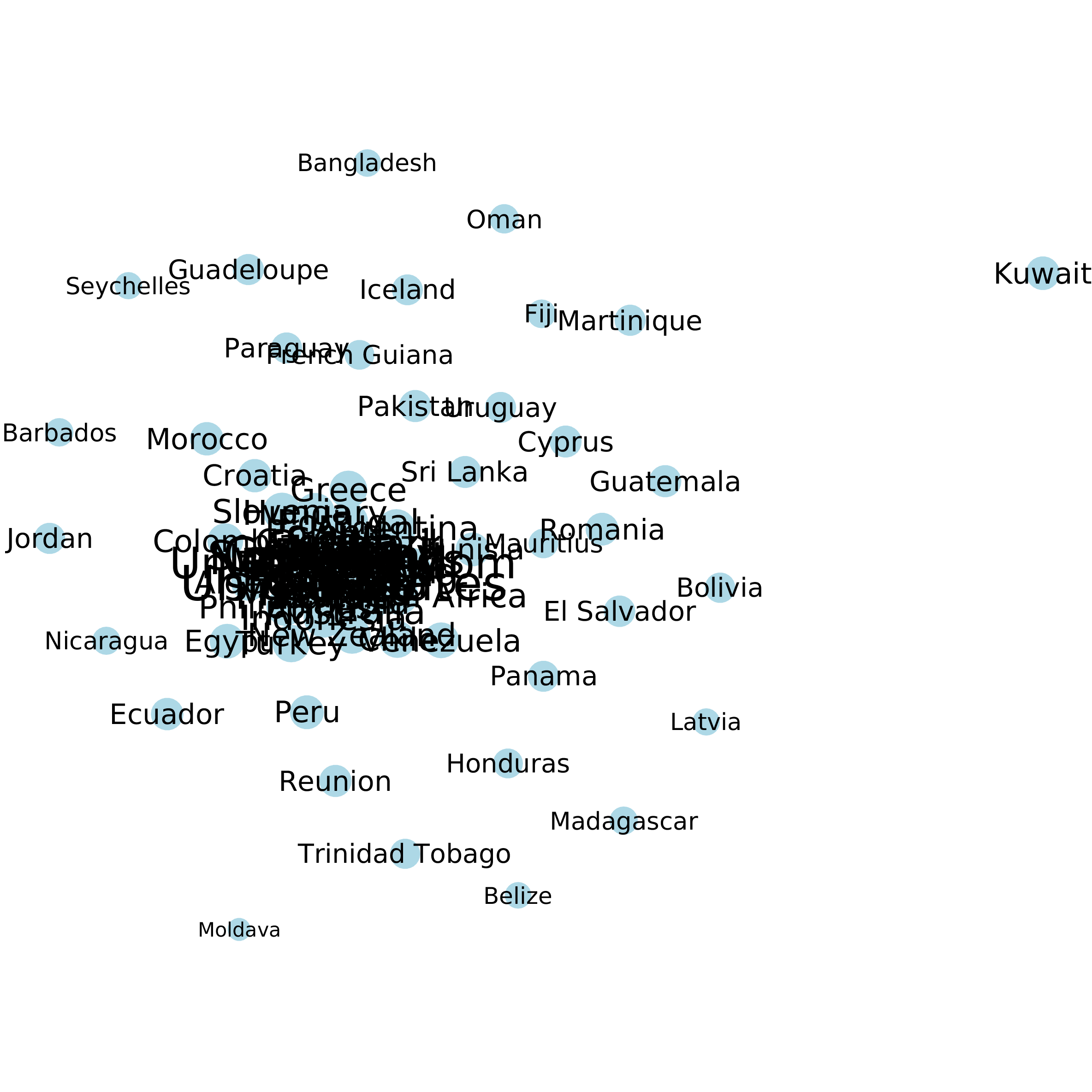
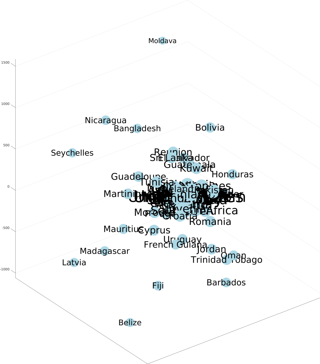
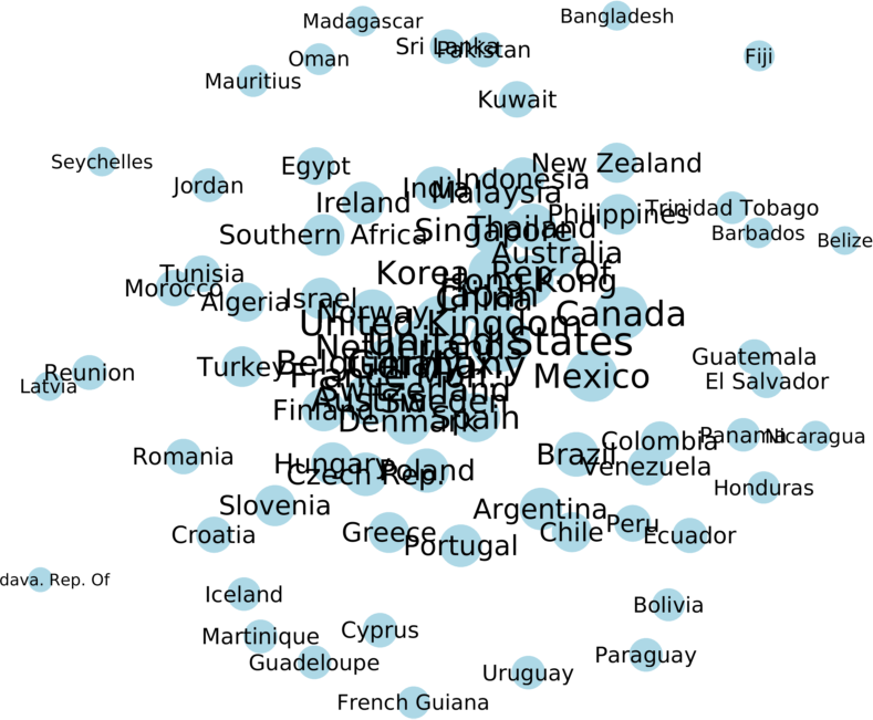
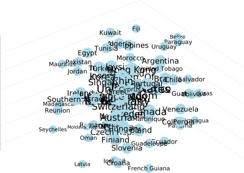
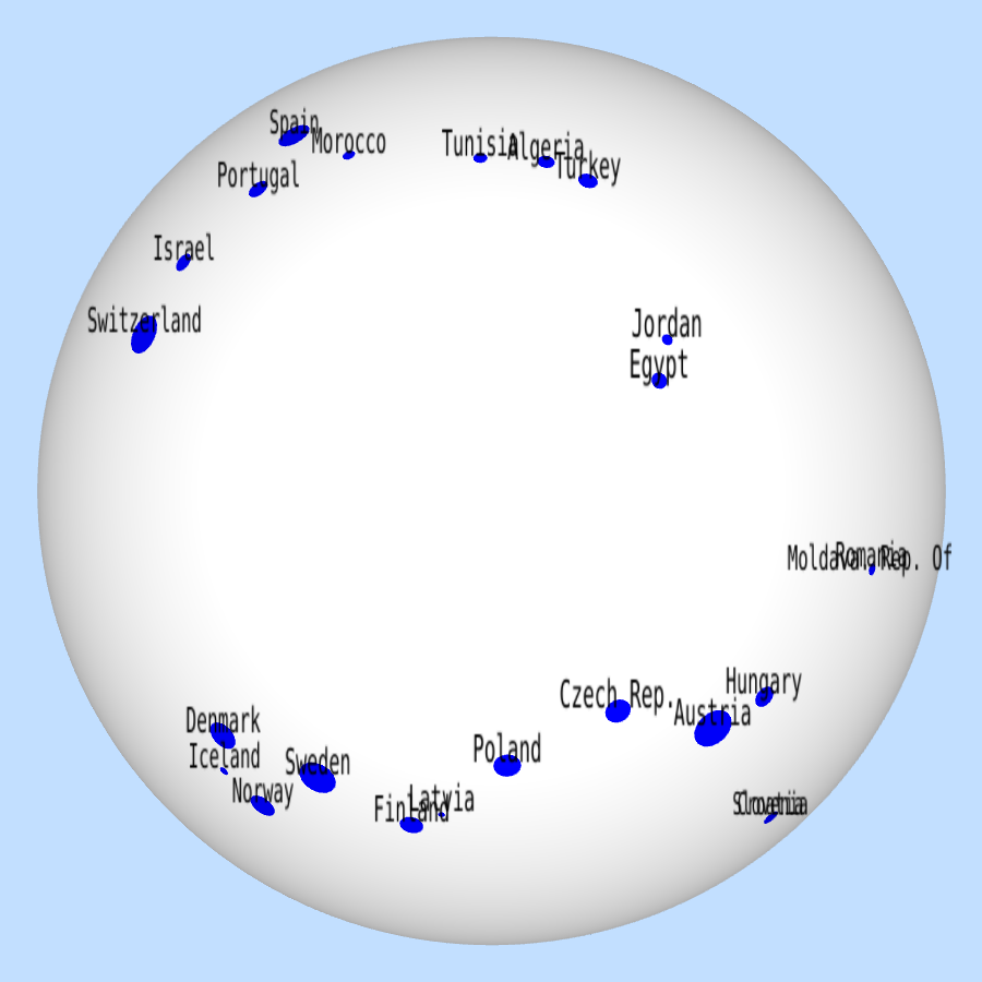
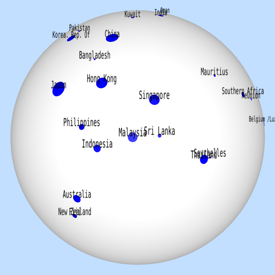
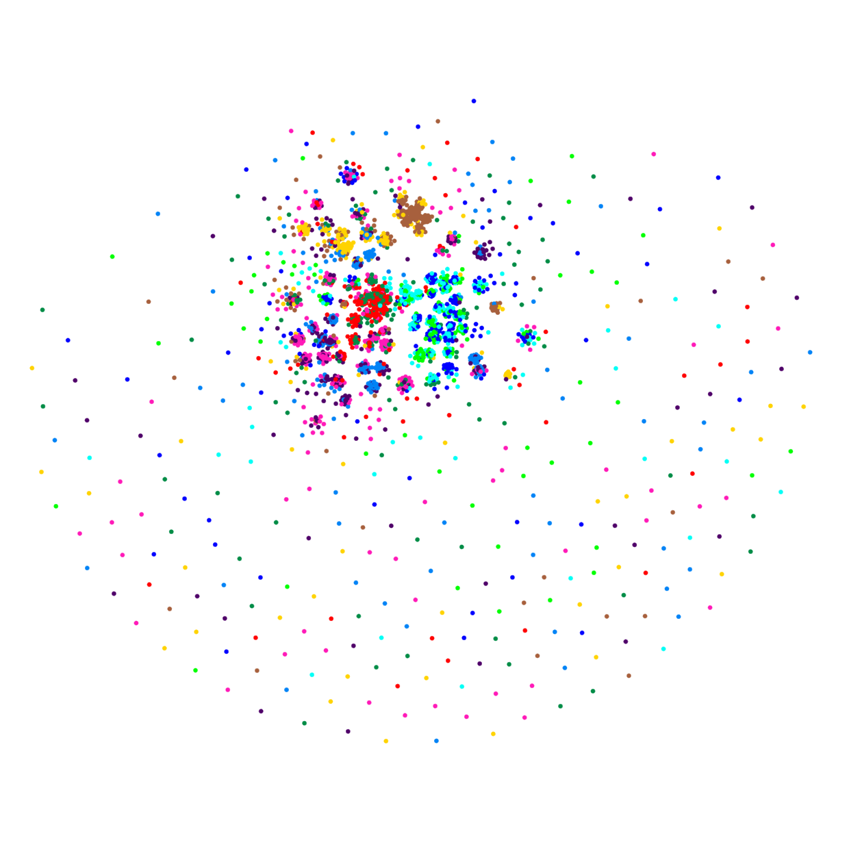
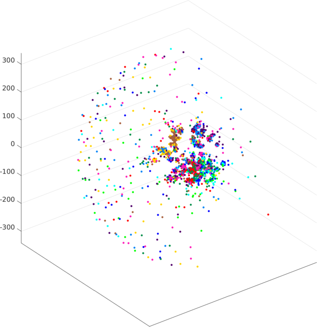
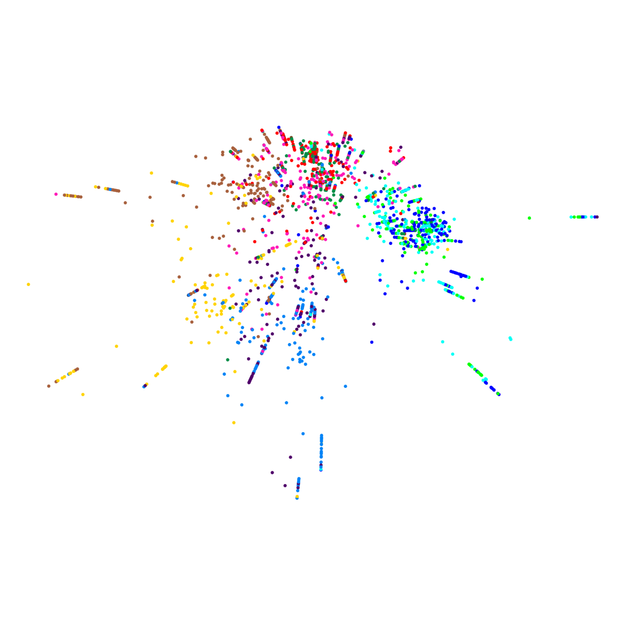
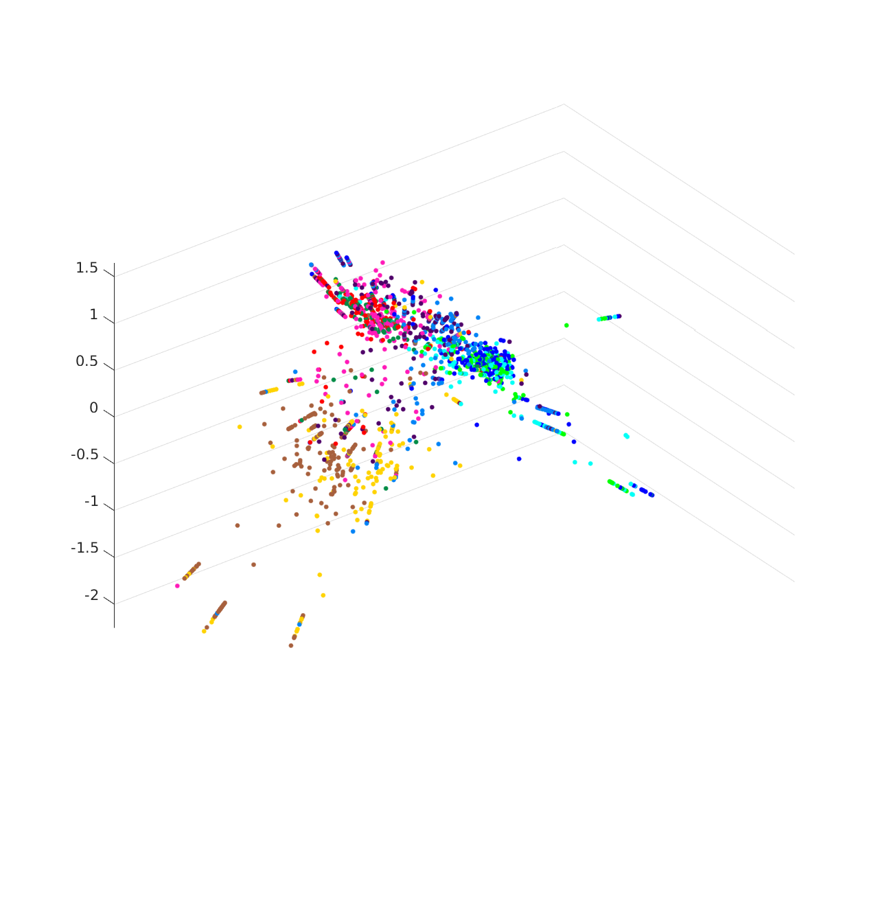
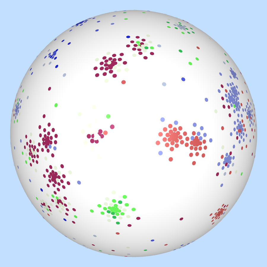
Figure 4 gives the visualizations of the MIREX dataset. In the panels (a) and (b), we can see that t-SNE caused over 90 percent of songs crowded in the center. A similar crowding problem appears in the MDS visualizations (panels c and d). In contrast, DOSNES performs much better in terms of separating the song genres and their subgroups, as in Figure 4 (e) and (f).

(a) t-SNE 2D

(b) t-SNE 3D

(c) MDS 2D

(d) MDS 3D

(e) DOSNES (viewpoint 1)

(f) DOSNES (viewpoint 2)

Figure 4: Visualizations of the MIREX dataset.

6 Conclusions

We have presented a new visualization method for high-dimensional and graph data. The proposed DOSNES method is based on the Stochastic Neighbor Embedding principle but with two key improvements: we normalize the input similarity matrix to be doubly stochastic and replace the 2D Euclidean embedding space with spheres in 3D space. Empirical results show that our method significantly outperforms the state-of-the-art approach t-SNE in terms of resolving the crowding problem and preserving intrinsic similarities.

We will perform a more thorough theoretical study on the connection between doubly stochastic similarity matrix and spherical embedding. There could be many possibilities to improve the user interface of spherical visualization, for example, using spherical screens to further facilitate the data navigation.

Appendix A Proofs of Propositions in the Paper

Proposition A.1.

If

$$\sum_{j}\exp(-\|y_{i}-y_{j}\|^{2})=c$$ (9)

for $i=1...n$ and some $c>0$, where $y_{i}\in\mathbb{R}^{d}$, then

$$n\ln\frac{n}{c}\leq\sum_{j}\|y_{i}-y_{j}\|^{2}\leq n\ln\frac{n}{c-nb}$$ (10)

where $b=a+(1-a)m-m^{a}$, $m=\min_{j}\exp(-\|y_{i}-y_{j}\|^{2})$ and $a=\frac{\ln[\ln(1/m)/(1-m)]}{\ln(1/m)}$.

Proof.

Let

$$A =\frac{1}{n}\sum_{j}\exp(-\|y_{i}-y_{j}\|^{2})=\frac{c}{n}\quad(\text{arithmetic mean})$$ (11)

$$G =[\exp(-\sum_{j}\|y_{i}-y_{j}\|^{2})]^{1/n}\quad(\text{geometric mean})$$ (12)

For lower bound, we have

$$G \leq A$$ (14)

$$[\exp(-\sum_{j}\|y_{i}-y_{j}\|^{2})]^{1/n} \leq\frac{c}{n}$$ (15)

$$\exp(-\sum_{j}\|y_{i}-y_{j}\|^{2}) \leq(\frac{c}{n})^{n}$$ (16)

$$-\sum_{j}\|y_{i}-y_{j}\|^{2} \leq n\ln\frac{c}{n}$$ (17)

$$n\ln\frac{n}{c} \leq\sum_{j}\|y_{i}-y_{j}\|^{2}$$ (18)

For upper bound, by Tung Theorem (Tung, 1975), we have

$$A-G\leq am+(1-a)M-m^{a}M^{1-a}$$ (20)

where $m=\min_{j}\exp(-\|y_{i}-y_{j}\|^{2})$, $M=\max_{j}\exp(-\|y_{i}-y_{j}\|^{2})$ and

$$a=\frac{\ln[M/(M-m)\ln(M/m)]}{\ln(M/m)}$$ (21)

Since $\max_{j}\exp(-\|y_{i}-y_{j}\|^{2})=1$, we have

$$A-G\leq am+(1-a)-m^{a}$$ (22)

and

$$a=\frac{\ln[1/(1-m)\ln(1/m)]}{\ln(1/m)}$$ (23)

Let $b=am+(1-a)-m^{a}$, we have

$$G \geq A-b$$ (24)

$$[\exp(-\sum_{j}\|y_{i}-y_{j}\|^{2})]^{1/n} \geq\frac{c}{n}-b$$ (25)

$$n\ln\frac{n}{c-nb} \geq\sum_{j}\|y_{i}-y_{j}\|^{2}$$ (26)

∎

Proposition A.2.

If

$$\sum_{j}(1+\|y_{i}-y_{j}\|^{2})^{-1}=c$$ (27)

for $i=1...n$ and some $c>0$, where $y_{i}\in\mathbb{R}^{d}$, then

$$\frac{n^{2}}{c}-n\leq\sum_{j}\|y_{i}-y_{j}\|^{2}\leq\frac{n^{2}}{c}-n+n(b^{1/2}-1)^{2}$$ (28)

where $b=1+\max_{j}\|y_{i}-y_{j}\|^{2}$.

Proof.

Let

$$A =\frac{1}{n}\sum_{j}(1+\|y_{i}-y_{j}\|^{2})\quad(\text{arithmetic mean})$$ (29)

$$H =\frac{n}{\sum_{j}(1+\|y_{i}-y_{j}\|^{2})^{-1}}\quad(\text{harmonic mean})$$ (30)

For upper bound, we have

$$A \geq H=\frac{n}{c}$$ (32)

$$\frac{1}{n}\sum_{j}\|y_{i}-y_{j}\|^{2}+1 \geq\frac{n}{c}$$ (33)

$$\sum_{j}\|y_{i}-y_{j}\|^{2} \geq\frac{n^{2}}{c}-n$$ (34)

For lower bound, due to Meyer Theorem (Meyer, 1984), let $b=1+\max_{j}\|y_{i}-y_{j}\|^{2}$, then we have

$$A-H \leq(b^{1/2}-1)^{2}$$ (36)

$$\frac{1}{n}\sum_{j}(1+\|y_{i}-y_{j}\|^{2}) \leq\frac{n}{c}+(b^{1/2}-1)^{2}$$ (37)

$$\sum_{j}\|y_{i}-y_{j}\|^{2} \leq\frac{n^{2}}{c}-n+n(b^{1/2}-1)^{2}$$ (38)

∎

Proposition A.3.

If

$$\sum_{j}\|y_{i}-y_{j}\|^{2}=c$$ (39)

for $i=1...n$ and some $c>0$, where $y_{i}\in\mathbb{R}^{d}$ and $\sum_{i}y_{i}=0$, then

$$\|y_{1}\|^{2}=\|y_{2}\|^{2}=...=\|y_{n}\|^{2}.$$ (40)

Proof.

$$\sum_{j}\|y_{i}-y_{j}\|^{2} =c$$ (41)

$$\sum_{j}(\|y_{i}\|^{2}+\|y_{j}\|^{2}-2y_{i}^{T}y_{j}) =c$$ (42)

$$n\|y_{i}\|^{2}+\sum_{j}\|y_{j}\|^{2}-2y_{i}^{T}\sum_{j}y_{j} =c$$ (43)

$$n\|y_{i}\|^{2}+\sum_{j}\|y_{j}\|^{2} =c$$ (44)

$$\|y_{i}\|^{2} =(c-\sum_{j}\|y_{j}\|^{2})/n$$ (45)

Since $\sum_{j}\|y_{j}\|^{2}$ is independent of $i$, we have

$$\|y_{1}\|^{2}=\|y_{2}\|^{2}=...=\|y_{n}\|^{2}.$$ (46)

∎

Appendix B Related work

Normalizing a matrix to be doubly stochastic has been used to improve cluster analysis. Zass and Shashua proposed to improve spectral clustering by replacing the original similarity matrix by its closest doubly stochastic similarities under $L_{1}$ or Frobenius norm (Zass and Shashua, 2006). Wang et al. (2012) generalized the projection to the family of Bregman divergences. To our knowledge, DOSNES is the first method that applies doubly stochastic matrices to improve data visualization.

Spherical visualization has appeared earlier in the visualization literature. For example, Spherical Multidimensional Scaling replaces Euclidean embedding space in the classical MDS with the unit sphere (Cox and Cox, 1991). Similar replacement was used by Wilson et al. (2010); Fang et al. (2011); Lunga and Ersoy (2013). Lunga and Ersoy (2013) also changed the output similarities with the Exit distribution, although this makes the objective function non-smooth.

Our method has a critical difference from the above approaches: the DOSNES embedding space is not restricted to the unit sphere. This is advantageous in two aspects: 1) our objective function is smooth and there is no gradient overflow problem; 2) DOSNES does not require an explicit scale variable for $Y$ or kernel bandwidth variable for $Q$, which is difficult to optimize. The sphere radius in DOSNES is implicitly adapted during optimization (similar to the scale adaptation in SNE; Hinton and Roweis, 2002). Moreover, the embedding space in our method is continuous, unlike sperical SOM (Boudjemaï et al., 2003) or spherical GTM (Bishop et al., 1998) that use discrete layout of cells.

The DOSNES spherical layout roots in the use of doubly stochastic similarity matrix and aims at solving the crowding problem in SNE, not only to eliminate the border effect. DOSNES does not require that the input high-dimensional data must be on spheres. This is also quite different from the methods that embed high-dimensional spherical data to low-dimensional spherical one (Lunga and Ersoy, 2013; Wang and Wang, 2016).

Compared with hyperbolic visualizations (see e.g., Lamping et al., 1995; Munzner and Burchard, 1995), the DOSNES display and navigation are more natural for most viewers without comprehensive knowledge of the transformation models such as Klein or Poincaré.

In computational and graphical statistics, Wagaman and Levina (2009) proposed a bootstrap approach to constructing the neighborhood graph used by Isomap (Tenenbaum et al., 2000). Their method, however, is not extensible to existing graph or network data. In another work, Faraway (2012) discussed the backscoring mapping from the embedding to dissimilarities in the input space, though their work is restricted to classical multidimensional scaling and thus give no insight to handle imbalanced affinity matrix.

Appendix C Visualizations by Gaussian s-SNE

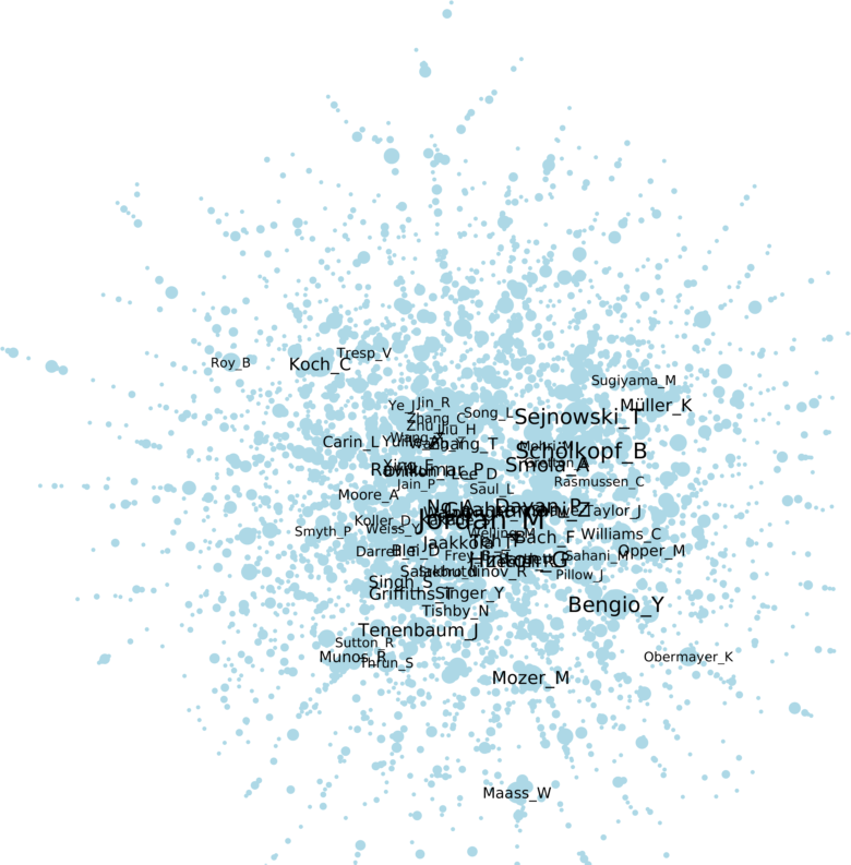
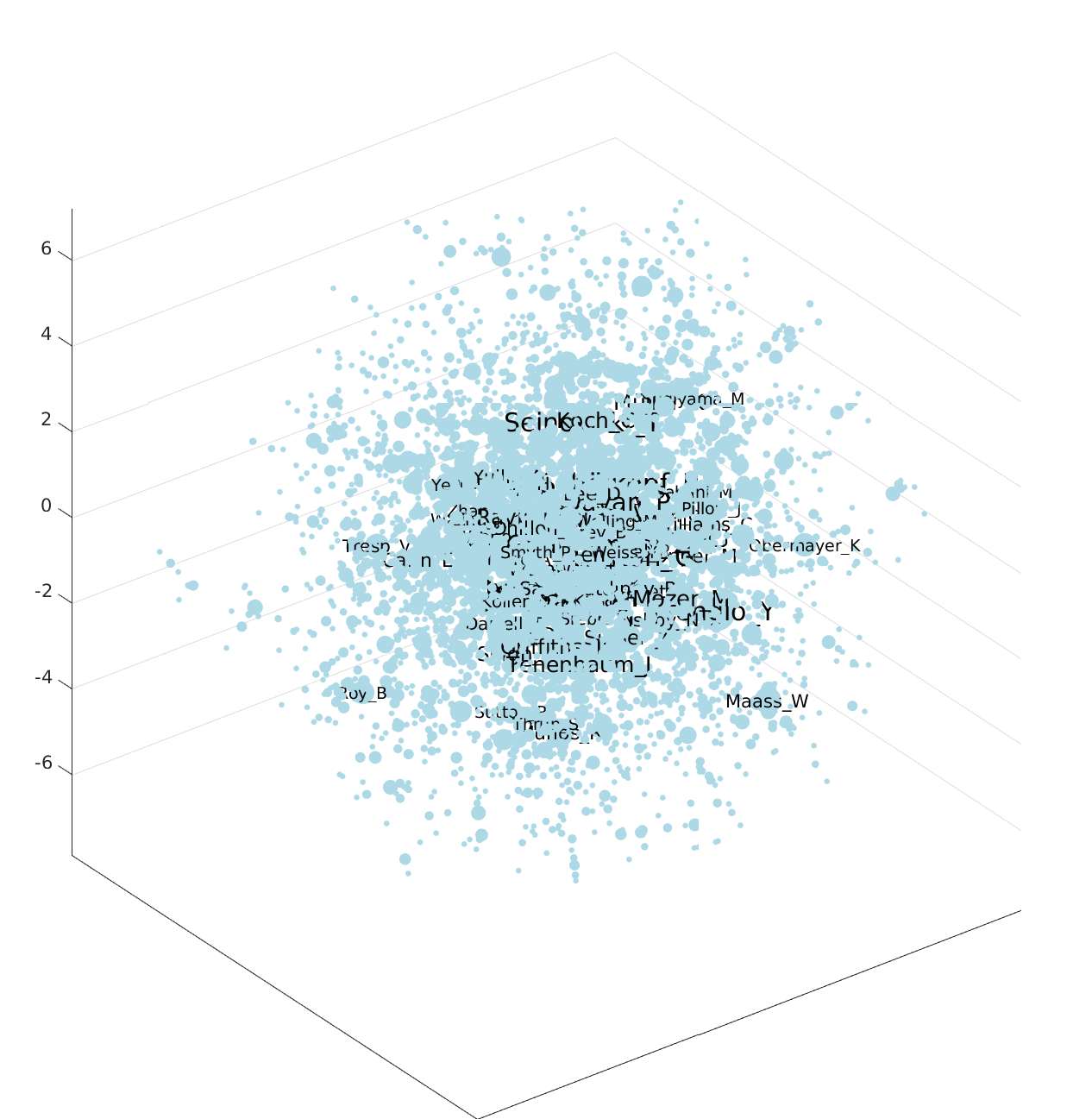
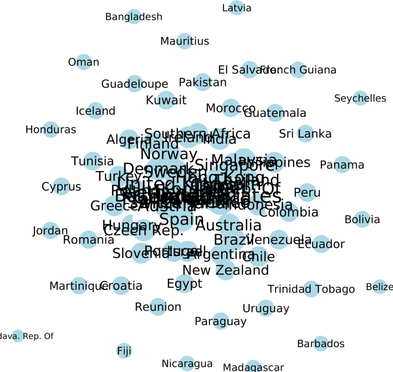
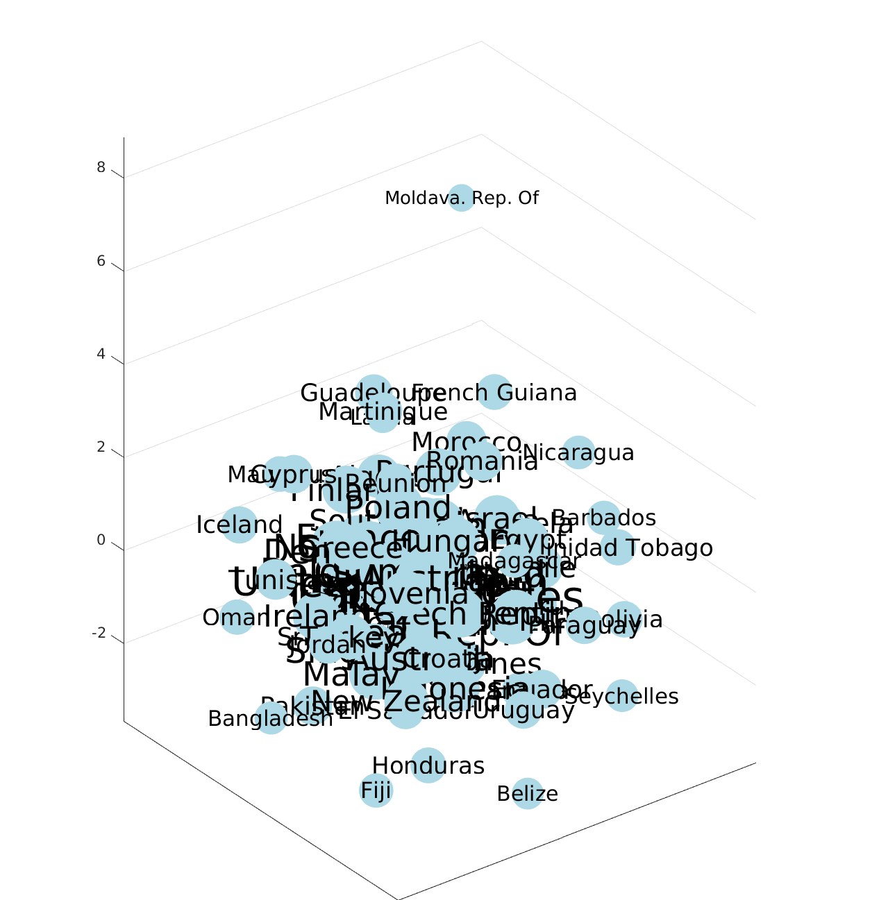
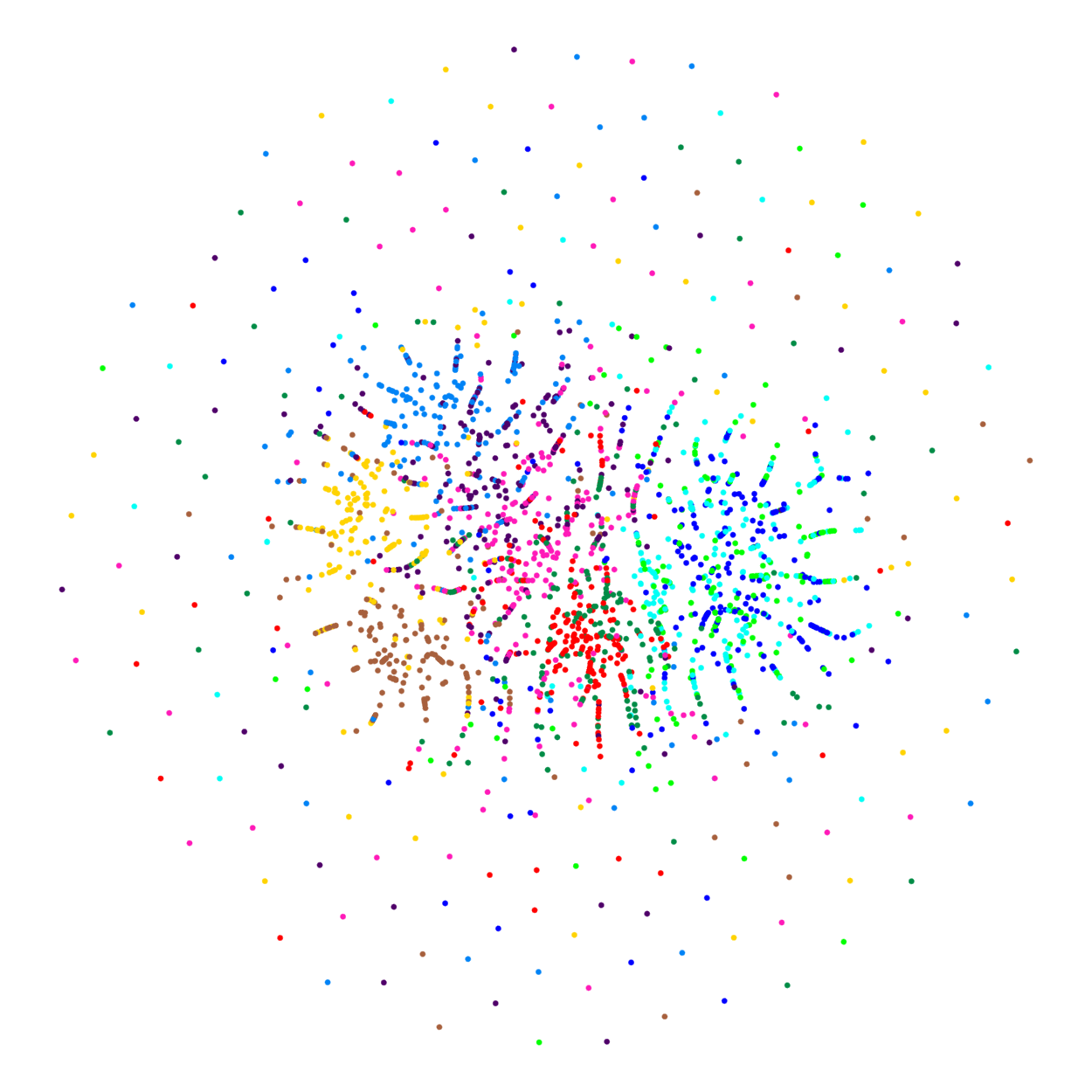
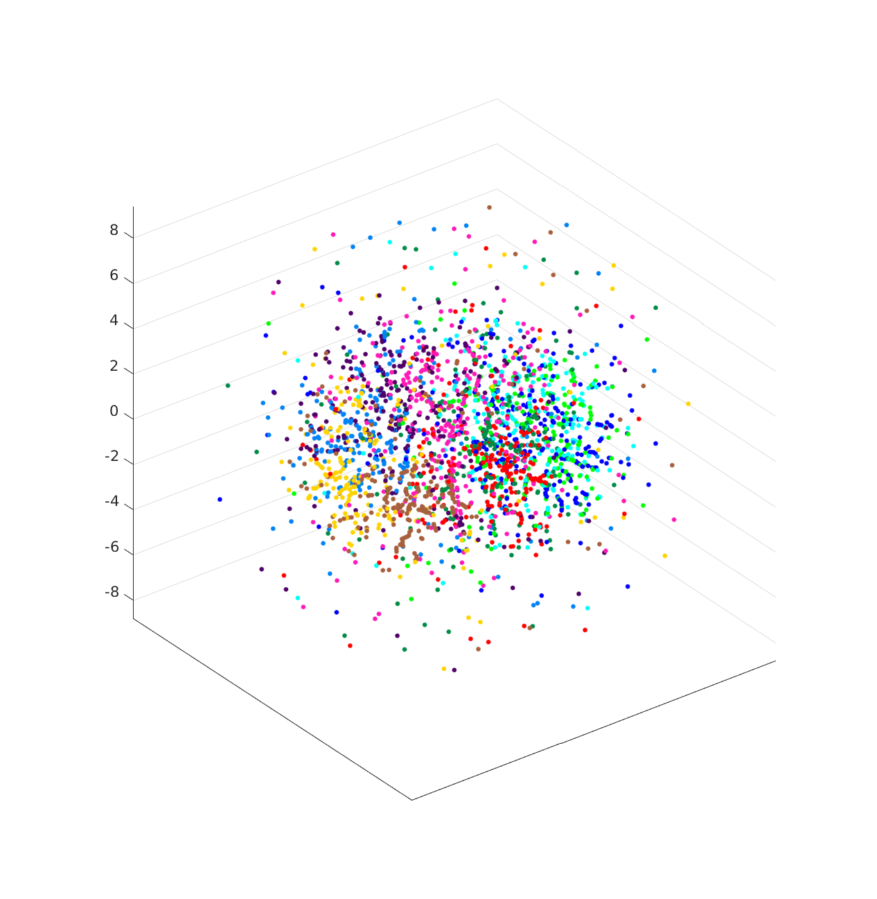
In the paper we show the visualizations by using s-SNE with the Cauchy kernel (i.e. t-SNE). Here we provide the results by using s-SNE with Gaussian kernel in Figure 5. We can see that the Gaussian s-SNE also suffer from the “crowding-in-the-center” problem, where many data nodes (points) with large degrees are crowded in the middle of the display. Same as t-SNE, The failure holds for both 2D and 3D Gaussian s-SNE. This further confirms the existence of “crowding problem” in s-SNE if the similairty matrix is not normalized.

(a) s-SNE 2D for NIPS

(b) s-SNE 3D for NIPS

(c) s-SNE 2D for WorldTrade

(d) s-SNE 3D for WorldTrade

(e) s-SNE 2D for MIREX

(f) s-SNE 3D for MIREX

Figure 5: Visualizations of the NIPS, WorldTrade, and MIREX data sets using s-SNE with Gaussian kernel: (left) 2D layout and (right) 3D layout.

References

- Belkin and Niyogi [2001] M. Belkin and P. Niyogi. Laplacian eigenmaps and spectral techniques for embedding and clustering. NIPS, 2001.
- Bishop et al. [1998] C. Bishop, M. Svensén, and C. Williams. GTM: the generative topographic mapping. Neural Computation, 1998.
- Boudjemaï et al. [2003] F. Boudjemaï, P. Enberg, and J. Postaire. Self organizing spherical map architecture for 3D object modeling. WSOM, 2003.
- Buja et al. [2008] A. Buja, D. F Swayne, M. Littman, N. Dean, H. Hofmann, and L. Chen. Data visualization with multidimensional scaling. Journal of Computational and Graphical Statistics, 2008.
- Cox and Cox [1991] T. Cox and M. Cox. Multidimensional scaling on a sphere. Communications in Statistics - Theory and Methods, 1991.
- Demartines and Hérault [1997] P. Demartines and J. Hérault. Curvilinear component analysis: a self-organizing neural network for nonlinear mapping of data sets. IEEE TNN, 1997.
- Fang et al. [2011] Y. Fang, M. Sun, S. Vishwanathan, and K. Ramani. sLLE: spherical locally linear embedding with applications to tomography. CVPR, 2011.
- Faraway [2012] J. Faraway. Backscoring in principal coordinates analysis. Journal of Computational and Graphical Statistics, 2012.
- Hinton and Roweis [2002] G. Hinton and S. Roweis. Stochastic neighbor embedding. NIPS, 2002.
- Iusem [2003] A. Iusem. On the convergence properties of the projected gradient method for convex optimization. Computational and Applied Mathematics, 2003.
- Lamping et al. [1995] J. Lamping, R. Rao, and P. Pirolli. A focus+context technique based on hyperbolic geometry for visualizing large hierarchies. CHI, 1995.
- Lawrence [2004] N. Lawrence. Gaussian process latent variable models for visualisation of high dimensional data. NIPS, 2004.
- Lunga and Ersoy [2013] D. Lunga and O. Ersoy. Spherical stochastic neighbor embedding of hyperspectral data. IEEE TGRS, 2013.
- Meyer [1984] B. Meyer. Some inequalities for elementary mean values. Mathematics of Computation, 1984.
- Munzner and Burchard [1995] T. Munzner and P. Burchard. Visualizing the structure of the world wide web in 3d hyperbolic space. VRML, 1995.
- Roweis and Saul [2000] S. Roweis and L. Saul. Nonlinear dimensionality reduction by locally linear embedding. Science, 2000.
- Sinkhorn and Knopp [1967] R. Sinkhorn and P. Knopp. Concerning nonnegative matrices and doubly stochastic matrices. Pacific Journal of Mathematics, 1967.
- Sun et al. [2015] K. Sun, J. Wang, A. Kalousis, and S. Marchand-Maillet. Space-time local embeddings. NIPS, 2015.
- Tang et al. [2016] J. Tang, J. Liu, M. Zhang, and Q. Mei. Visualizing large-scale and high-dimensional data. WWW, 2016.
- Tenenbaum et al. [2000] J. Tenenbaum, V. de Silva, and J. Langford. A global geometric framework for nonlinear dimensionality reduction. Science, 2000.
- Torgerson [1952] W. Torgerson. Multidimensional scaling: I. theory and method. Psychometrika, 1952.
- Tung [1975] S. Tung. On lower and upper bounds of the difference between the arithmetic and the geometric mean. Mathematics of Computation, 1975.
- van der Maaten [2014] L. van der Maaten. Accelerating t-SNE using tree-based algorithms. JMLR, 2014.
- van der Maaten and Hinton [2008] L. van der Maaten and G. Hinton. Visualizing data using t-SNE. JMLR, 2008.
- van der Maaten et al. [2009] L. van der Maaten, E. Postma, and J. van den Herik. Dimensionality reduction: a comparative review. JMLR, 2009.
- Vladymyrov and Carreira-Perpiñán [2013] M. Vladymyrov and M. Carreira-Perpiñán. Entropic affinities: Properties and efficient numerical computation. ICML, 2013.
- Wagaman and Levina [2009] A. Wagaman and E. Levina. Discovering sparse covariance structures with the isomap. Journal of Computational and Graphical Statistics, 2009.
- Wang et al. [2012] F. Wang, P. Li, A. König, and M. Wan. Improving clustering by learning a bi-stochastic data similarity matrix. Know. and Info. Sys., 2012.
- Wang and Wang [2016] M. Wang and D. Wang. VMF-SNE: embedding for spherical data. ICASSP, 2016.
- Wilson et al. [2010] R. Wilson, E. Hancock, E. Pekalska, and R. Duin. Spherical embeddings for non-euclidean dissimilarities. CVPR, 2010.
- Yang et al. [2014] Z. Yang, J. Peltonen, and S. Kaski. Optimization equivalence of divergences improves neighbor embedding. ICML, 2014.
- Zass and Shashua [2006] R. Zass and A. Shashua. Doubly stochastic normalization for spectral clustering. NIPS, 2006.