Optimal-order isogeometric collocation at Galerkin superconvergent points

Abstract

In this paper we investigate numerically the order of convergence of an isogeometric collocation method that builds upon the least-squares collocation method presented in [1] and the variational collocation method presented in [2]. The focus is on smoothest B-splines/NURBS approximations, i.e, having global $C^{p-1}$ continuity for polynomial degree $p$. Within the framework of [2], we select as collocation points a subset of those considered in [1], which are related to the Galerkin superconvergence theory. With our choice, that features local symmetry of the collocation stencil, we improve the convergence behaviour with respect to [2], achieving optimal $L^{2}$-convergence for odd degree B-splines/NURBS approximations. The same optimal order of convergence is seen in [1], where, however a least-squares formulation is adopted. Further careful study is needed, since the robustness of the method and its mathematical foundation are still unclear.

Keywords

isogeometric analysis, B-splines, NURBS, collocation method, superconvergent points.

1 Introduction

The splines-based collocation method for solving differential equations has about fifty years of history. The first references are [3, 4], where cubic $C^{2}$ splines are used to solve a second order two-point boundary value problem. In particular, in order to achieve optimal convergence, [4] collocates a modified equation, where the modification is obtained by constructing a suitable interpolant of the true solution. An extension of this approach to multivariate (tensor-product) splines and partial differential equations is studied in [5], while extensions to $m$-order differential equations are found in [6] and in particular in [7], where the optimality of the method is achieved by collocating the original, unperturbed, equation at suitably selected collocation points, i.e, Gaussian quadrature points. The method only works for splines of continuity $C^{m-1}$ and degree $m+k-1$, with $k\geq m$. Splines-based collocation has been successfully applied also to integro-differential equations on curves, and to the boundary element method for planar domains (see [8] and references therein).

The interest and development of splines-based collocation methods for partial differential equations has been driven in the last decade by isogeometric analysis (see [9, 10, 11, 12, 13, 14, 15, 16, 17, 18, 19, 20, 21, 22, 2] and references therein). The motivation is computational efficiency: isogeometric collocation is more efficient than the isogeometric Galerkin method, at least for standard code implementations, see [23]. In particular, the assembly of system matrices is much faster for collocation than for Galerkin (unless one adopts recent quadrature algorithms as in [24]). On the other hand, contrary to the Galerkin method, isogeometric collocation based on maximal regularity splines has always been reported suboptimal in literature, when the error is measured in $L^{2}$ or $L^{\infty}$ norm. For example, the $L^{2}$ norm of the error of the collocation method at Greville points, studied in [11] for a second-order elliptic problem, converges under $h$-refinement as $O(h^{p-1})$ or $O(h^{p})$, when the degree $p$ is odd or even, respectively, while the optimal interpolation error is $O(h^{p+1})$ regardless of the parity of $p$ for a smooth solution. We remark that the previous ideas of [4, 7] cannot be applied directly to the isogeometric case since [4] would require a complex modification of the equation (this approach however deserves further investigation) and [7] does not work for maximal smoothness splines, which represent the most interesting choice in this framework.

Collocating the equation at Greville points (obtaining the method to which we refer here as Collocation at Greville Points, C-GP) is a common choice since Greville points are classical interpolation points for arbitrary degree and regularity splines, well studied in literature, see e.g. [25]. There is however an alternative and interesting approach, from [1] and [2]. In particular, [2] introduces an ideal collocation scheme whose solution coincides with the solution of the Galerkin method, thus recovering optimal convergence. This scheme uses as collocation points the so-called Cauchy-Galerkin points, a well-chosen subset of the zeros of the Galerkin residual. These points are not known a-priori, and therefore [2] selects as approximated Cauchy-Galerkin points the points where, under some hypotheses (we will return on this point later on, in Section 3.3), one can prove superconvergence of the second derivatives of the Galerkin solution. Indeed, for a Poisson problem the residual is equivalent to the error on the approximation of the second derivatives. This is an idea from the previous paper [1]: if we constrain the numerical residual to be zero where the Galerkin residual is estimated to be zero up to higher order terms, then the computed numerical solution is expected to be close to the Galerkin numerical solution up to higher order terms as well. There are however two difficulties: the first and most relevant one is that also the superconvergent points are not known with enough accuracy everywhere in the computational domain; the second one is that there are more Galerkin superconvergent points than degrees-of-freedom, $n_{dof}$, for maximal smoothness splines (the superconvergent points are about $2n_{dof}$). Indeed, [1] proposes to compute a solution of the overdetermined linear system by a least-square approximation. This approach, which is more expensive than collocation, achieves optimal convergence for odd degrees and one-order suboptimal for even degrees. We refer to it as Least-Squares approximation at Superconvergent Points (LS-SP). Instead, [2] designs a well-posed collocation scheme by selecting only $n_{dof}$ collocation points among those used in [1]. Roughly speaking, one superconvergent point per element is used as collocation point, i.e., one every other superconvergent point (as shall be clearer later), and therefore in this paper we denote this method as Collocation at Alternating Superconvergent Points (in short C-ASP). The $L^{2}$ convergence of C-ASP is one-order suboptimal for any degree, i.e., the $L^{2}$-error decays as $O(h^{p})$ for any $p$, which means that the lack of accuracy in the estimated location of the superconvergent points affects the convergence behaviour of the collocation method C-ASP.

However, we have an interesting and useful finding to report in this paper. In the framework of [2], we propose a new criterion for selecting the subset of superconvergent points, which features local symmetry and gives improved convergence properties compared to C-ASP. Roughly speaking, we propose to take two (symmetric) superconvergent points in every other element. This method, which we refer to as Clustered Superconvergent Points (C-CSP), features the same convergence order as the LS-SP approach, i.e., optimal convergence for odd degrees in $L^{2}$ and $L^{\infty}$ norm. Thus, we finally have an optimally convergent isogeometric collocation scheme with cubic $C^{2}$ splines (see [23] for a discussion on the relevance of this case).

The results we have obtained are preliminary and, while some “magical” error cancellation happens with the C-CSP collocation point selection, perhaps due to the local symmetry of the collocation stencil, we are still unable to provide a rigorous convergence proof for C-CSP (nor for LS-SP or C-ASP). Furthermore, we have considered quite simple numerical benchmarks, therefore the numerical evidence that we have gathered is not yet conclusive regarding the robustness of the method. C-CSP definitely deserves further analysis.

The outline of this work is as follows. Section 2 is a quick overview on B-splines, NURBS, and isogeometric analysis. In Section 3 we present a framework for isogeometric collocation and the collocation schemes C-GP, LS-SP, C-ASP, and the new C-CSP. In Section 4 we show some numerical tests of C-CSP, focusing on the odd degree case, discuss its robustness and compare it with the other collocation methods. Finally, some conclusions and perspectives on future works are detailed in Section 5.

2 Preliminaries

2.1 B-splines

Let us consider an interval $\hat{\Omega}\subset\mathbb{R}$. The B-splines basis functions defined on $\hat{\Omega}$ are piecewise polynomials that are built from a knot vector, i.e., a vector with non-decreasing entries $\Xi=[\xi_{1},\xi_{2}...,\xi_{n+p+1}]$, where $n$ and $p$ are, respectively, the number of basis functions that will be built from the knot vector and their polynomial degree. We name element a knot span $(\xi_{i},\xi_{i+1})$ having non-zero length, and we denote by $h$ the maximal length (the meshsize). A knot vector is said to be open if its first and last knot have multiplicity $p+1$, i.e., each of them is repeated $p+1$ times.

Following [25] and given a knot vector $\Xi$, univariate B-splines basis functions $N_{i,p}$ are defined recursively as follows for $i=1,\ldots,n$:

$$N_{i,0}(\xi)=\begin{cases}1,&\xi_{i}\leq\xi<\xi_{i+1},\\ 0,&\textrm{otherwise},\\ \end{cases}$$ (2.1)

$$N_{i,p}(\xi)=\begin{cases}\dfrac{\xi-\xi_{i}}{\xi_{i+p}-\xi_{i}}N_{i,p-1}(\xi)+\dfrac{\xi_{i+p+1}-\xi}{\xi_{i+p+1}-\xi_{i+1}}N_{i+1,p-1}(\xi),&\xi_{i}\leq\xi<\xi_{i+p+1},\\ 0,&\textrm{otherwise,}\end{cases}$$

where we adopt the convention $\dfrac{0}{0}=0$; note that the basis corresponding to an open knot vector will be interpolatory in the first and last knot.

Remark 2.1.

In this work we only consider knot vectors whose internal knots have multiplicity one: the associated B-splines/NURBS have then global $C^{p-1}$ regularity.

We define by $\hat{S}^{p}=\textrm{span}\{N_{i,p}|i=1,...,n\}$ the space spanned by B-splines of degree $p$ and regularity $p-1$, built from a given knot vector $\Xi$. We also introduce the space of periodic B-splines, spanning the space $\widetilde{S}^{p}=\{v\in\hat{S}^{p}|v(0)=v(1),\ v^{\prime}(0)=v^{\prime}(1),...,\ v^{(p-1)}(0)=v^{(p-1)}(1)\}$; interestingly, the dimension of $\widetilde{S}^{p}$ equals the number of elements of the underlying knot vector $\Xi$, a property that will come in handy later on.

Multivariate splines spaces can be constructed from univariate spaces by means of tensor products. For example, a B-splines space in two dimensions can be defined by considering the knot vectors $\Xi=[\xi_{1},\xi_{2}...,\xi_{n+p+1}]$ and $\Lambda=[\eta_{1},\eta_{2},...,\eta_{m+q+1}]$, and defining $\hat{S}^{p,q}=\textrm{span}\{N_{i,p}(\xi)M_{j,q}(\eta),i=1,...,n,j=1,...,m\}$. In the following, it will be useful to refer to the basis functions spanning $\hat{S}^{p,q}$ with a single running index $k$ ranging from $1$ to $n\times m$, i.e.

$$\hat{S}^{p,q}=\textrm{span}\{\varphi_{k}^{p,q}(\xi,\eta)=N_{i,p}(\xi)M_{j,q}(\eta)\,|\,k=i+(j-1)m,\,i=1,\ldots,n,\,j=1,\ldots,m\}.$$ (2.2)

2.2 NURBS

Non-uniform rational B-splines (NURBS, cf. [26]) are defined for the purpose of describing geometries of practical interest like conic sections, see e.g. Problem 3 in next section. The definition of a generic bivariate NURBS function on the parametric square $\hat{\Omega}$ is

$$\forall(\xi,\eta)\in\hat{\Omega},\quad R_{i,j}^{p,q}(\xi,\eta)=\dfrac{N_{i,p}(\xi)M_{j,q}(\eta)w_{i,j}}{\sum_{\widehat{i}=1}^{n}\sum_{\widehat{j}=1}^{m}N_{\widehat{i},p}(\xi)M_{\widehat{j},q}(\eta)w_{\hat{i},\hat{j}}}\forall i=1,...,n,\forall j=1,...,m$$

where $w_{i}$ are suitable weights, and $N_{i,p}(\xi),M_{j,q}(\eta)$ are the univariate B-splines basis functions defined in (2.1). Similarly to (2.2) we also introduce a single running index $k=1,\ldots,n\times m$ to refer to the NURBS basis, i.e.,

$$R_{k}^{p,q}(\xi,\eta)=R_{i,j}^{p,q}(\xi,\eta),\text{ with }k=i+(j-1)m,\,i=1,\ldots,n,\,j=1,\ldots,m.$$

3 Isogeometric collocation and the choice of the collocation points

3.1 Isogeometric collocation

In our numerical tests we will consider both one-dimensional and two-dimensional elliptic problems, which we now introduce.

Problem 1 (One-dimensional Dirichlet boundary problem).

Find $u:[0,1]\rightarrow\mathbb{R}$ such that

$$\begin{cases}u^{\prime\prime}(x)+a_{1}(x)u^{\prime}(x)+a_{0}(x)u(x)=f(x)\ \ \ \forall x\in(0,1)\\ u(0)=u(1)=0\end{cases}$$ (3.1)

where $a_{0},a_{1},f:[0,1]\rightarrow\mathbb{R}$ are sufficiently regular functions.

We assume that this problem has a unique smooth solution. We then look for an approximate solution $u_{h}(x)=\sum_{i=1}^{n}c_{i}N_{i,p}(x)\in\hat{S}^{p}$, that complies with the boundary conditions $u(0)=u(1)=0$ (i.e. $c_{1}=c_{n}=0$, given the interpolatory property of open knot vectors at the first and last knot), and that satisfies (3.1) in $n-2$ collocation points $\{\tau_{1},...,\tau_{n-2}\}$ that need to be specified, i.e.

$$u_{h}^{\prime\prime}(\tau_{i})+a_{1}u_{h}^{\prime}(\tau_{i})+a_{0}u_{h}(\tau_{i})=f(\tau_{i}),\qquad\forall i=1,...,n-2.$$ (3.2)

The coefficients $c_{2},\ldots,c_{n-1}$ are then computed by solving the linear system obtained by inserting the expansion $u_{h}(x)=\sum_{i=1}^{n}c_{i}N_{i,p}(x)$ into (3.2). We also shall introduce a periodic version of Problem 1, which we consider because it is particularly simple to set up a collocation scheme for it, due to the already-mentioned fact that the number of degrees-of-freedom $n$ of $\widetilde{S}^{p}$ (hence the number of collocation points to be used) is identical to the number of elements of $\Xi$.

Problem 2 (One-dimensional periodic boundary problem).

Find $u:\mathbb{R}\rightarrow\mathbb{R}$ such that

$$\begin{cases}u^{\prime\prime}(x)+a_{1}u^{\prime}(x)+a_{0}u(x)=f(x)&\forall x\in\mathbb{R},\\ u(x)=u(1+x)&\forall x\in\mathbb{R},\end{cases}$$ (3.3)

where $a_{0},a_{1}$ and $f$ are sufficiently regular periodic functions.

We assume again that this problem has a unique (periodic) smooth solution. Note that the periodic problem is not well-posed if $a_{0}$ is null. The B-splines approximation of the solution of (3.3) is therefore $u_{h}\in\widetilde{S}^{p}$ such that

$$u_{h}^{\prime\prime}(\tau_{i})+a_{1}u_{h}^{\prime}(\tau_{i})+a_{0}u_{h}(\tau_{i})=f(\tau_{i})\qquad\forall i=1,...,n,$$ (3.4)

for suitably chosen collocation points $\{\tau_{1},...,\tau_{n}\}$ with periodic distribution on $[0,1]$.

Finally, we also consider the two-dimensional Poisson equation, that we will solve by a multivariate collocation scheme constructed by tensorizing univariate sets of collocation points. More specifically, we denote by $\Omega\subset\mathbb{R}^{2}$ a domain described by a NURBS parametrization $\mathbf{F}:\hat{\Omega}\rightarrow\Omega$, where $\hat{\Omega}=[0,1]\times[0,1]$ and

$$\mathbf{F}(\xi,\eta)=\sum_{k=1}^{n\times m}\mathbf{P}_{k}R_{k}^{p,q}(\xi,\eta),\quad\mathbf{P}_{k}\in\mathbb{R}^{2},$$

we let $\Gamma$ denote the boundary of $\Omega$, and we consider the Dirichlet problem

Problem 3 (Two-dimensional Dirichlet boundary problem).

Find $u:\Omega\rightarrow\mathbb{R}$ such that

$$\begin{cases}-\Delta u=f&\textrm{in}\ \Omega,\\ u=0&\textrm{on}\ \Gamma,\end{cases}$$ (3.5)

where $f:\Omega\rightarrow\mathbb{R}$ is a sufficiently regular function.

Again, we assume that this problem has a unique smooth solution. Following the isogeometric paradigm, the discrete solution $u_{h}$ is sought in the isogeometric space

$$u_{h}\in S^{p,q}=\text{span}\left\{R_{k}^{p,q}\circ\mathbf{F}^{-1},\,\forall k=i+(j-1)m,\,i=1,...,n,\,j=1,...,m\right\}$$

cf. (2.2), and the collocation points are the image through $\mathbf{F}(\cdot)$ of a tensor-product grid of collocation points on $[0,1]^{2}$. The collocation method is then obtained as for the univariate case.

3.2 Greville points and C-GP

Greville points, or abscissas, for $p$-degree B-splines associated to a knot vector $\Xi=\{\xi_{1},...,\xi_{n+p+1}\}$ are defined as

$${\tau^{GP}_{i}}=\frac{\xi_{i+1}+...+\xi_{i+p}}{p},\quad\forall i=1,...,n,$$

see Figure 1 for an example computed from a open uniform knot vector and degree $p=3$ and $p=4$. For an open knot vector the first and last Greville point coincide with the first and last knot $\xi_{1}$ and $\xi_{n+p+1}$. A common collocation scheme for second-order boundary value problems, as proposed in [11], uses as collocation points the $n-2$ internal Greville points. For brevity, this is denoted Collocation at Greville Points, C-GP.

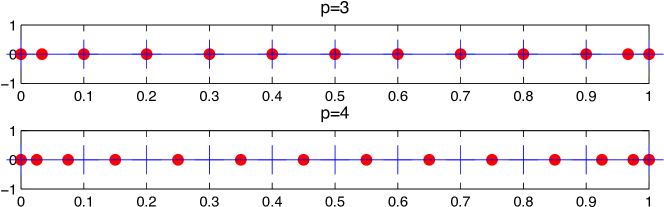
Figure 1: Examples of Greville points computed from an open knot vector: p=3 and p=4. The interior Greville points are used as collocation points in the C-GP scheme.

	Galerkin	C-GP		LS-SP and C-CSP		C-ASP
		Odd $p$	Even $p$	Odd $p$	Even $p$
$L^{2}$	$p+1$	$p-1$	$p$	$p+1$	$p$	$p$
$H^{1}$	$p$	$p-1$	$p$	$p$	$p$	$p$
$H^{2}$	$p-1$	$p-1$	$p-1$	$p-1$	$p-1$	$p-1$

Table 1: Comparisons of orders of convergence: Galerkin, C-GP, LS-SP, C-CSP and C-ASP.

In Table 1 we report the orders of convergence of C-GP and of the other methods considered in this paper. The convergence rate of C-GP in $L^{2}$ norm is $p-1$ when odd degree are used and $p$ when even degree B-Splines are used as discussed earlier (i.e. two-orders and one-order suboptimal, respectively). The error in $H^{1}$ norm converges with the same orders of the $L^{2}$ norm, and is therefore optimal for even degrees and one-order suboptimal for odd degrees. The error measured in $H^{2}$ norm is instead optimal for every degree.

3.3 Cauchy-Galerkin points and superconvergent points for the second derivative of the Galerkin solution

Following [2] and [1], we now introduce the Cauchy-Galerkin points and the second-derivative superconvergent points for the Galerkin solution of Problem 1, which will be used to construct a collocation or least-squares method. Assume for a moment that $a_{0}=a_{1}=0$ in Problem 1, i.e., consider

$$\begin{cases}-u^{\prime\prime}(x)=f(x)&\ \ \ \forall x\in(0,1)\\ u(0)=u(1)=0,\end{cases}$$ (3.6)

and let $u_{h}^{*}$ be the approximated solution given by the Galerkin method based on B-splines. The Cauchy-Galerkin points are collocation points where the Galerkin residual, in this case $D^{2}(u-u_{h}^{*})$, is zero. Since these points are unknown a-priori, one can look for a high-order approximation of them, i.e, the so-called superconvergent points. In general, the points $\Psi_{h}=\{\psi_{h,1},...,\psi_{h,w}\}$ with $w\in\mathbb{N},w>0,$ are said to be superconvergent points for the $j$-th derivative of $u$ if

$$\Big{[}\sum_{\psi_{h,i}\in\Psi_{h}}\big{[}D^{j}(u-u_{h}^{*})(\psi_{h,i})\big{]}^{2}\Big{]}^{\frac{1}{2}}\leq Ch^{p+1-j+k},\quad\forall i=1\ldots,w,$$ (3.7)

where $k>0$, $j\geq 0$, $C$ is a constant, $h$ is the meshsize of the knot vector, and $p$ is the degree of the B-splines. Here we are therefore interested in the case $k=1$ and $j=2$.

Degree	Second derivative SP
p=3	$\frac{-1}{\sqrt{3}},\frac{1}{\sqrt{3}}$
p=4	-1,0,1
p=5	$\pm\frac{\sqrt{225-30\sqrt{30}}}{15}$
p=6	-1,0,1
p=7	$\pm 0.504918567512$

Table 2: On the reference element $[-1,1]$, location of superconvergent points for the second derivative (from [2]).

Finding the location of the superconvergent points is in general an open problem as well. Under the assumption that the superconvergent points are element-invariant (i.e., images by affine mapping of points on a reference element) their locations have been estimated in [2] and are reported in Table 2 for a reference element $[-1,1]$. The same points are estimated in [1] under a similar periodicity assumption. Both assumptions do not hold true in many cases of interest. An alternative superconvergence theory can be found in [27], based on a mesh symmetry assumption; this hypothesis however does not hold true for elements close to the boundary.

Following [1] and [2], since we do not have access to the “true” superconvergent points, we use the points in Table 2, linearly mapped to the generic element, as “surrogate” superconvergent points in one-dimension. How well do these “surrogate” superconvergent points approximate the Cauchy-Galerkin points? This is the main question and some qualitative answer can be found in Figures 2 and 3, that show $D^{2}(u-u_{h}^{*})$ for equation (3.6) with $f(x)=\sin(\pi x)$, over a mesh with $10$ and $20$ elements and $p=3,\ldots,7$, as well as the “surrogate” superconvergent points for each degree of approximation: for odd degrees, a non-negligible discrepancy is evident at the boundaries of the domain, and for even degrees this occurs also at the middle of the interval. Figure 4 is a zoom of the first element in Figure 3. For completeness, Figure 5 shows the residual for the Periodic Problem 2 with $a_{0}=a_{1}=1$, and $f(x)=(1+4\pi^{2})\sin(\pi x)+2\pi\cos(2\pi x)$ over a mesh with 10 elements and $p=3,\ldots,7$, as well as the “surrogate” superconvergent points for each degree of approximation. In this case, the mismatch between the zeros of the residual and the “surrogate” superconvergent points is higher in correspondence of a smaller residual. Note that the residual is not periodic at the element scale.

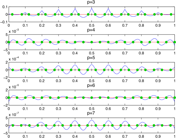
Figure 2: Plot of $D^{2}(u-u_{h}^{*})$, equivalent to the residual of problem (3.6), and “surrogate” superconvergent points (green dots), on a mesh with 10 elements.

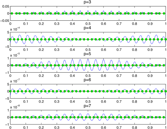
Figure 3: Plot of $D^{2}(u-u_{h}^{*})$, equivalent to the residual of problem (3.6), and “surrogate” superconvergent points (green dots), on a mesh with 20 elements.

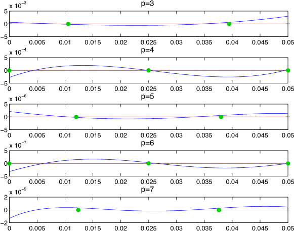
Figure 4: Zoom on the first element of Figure 3.

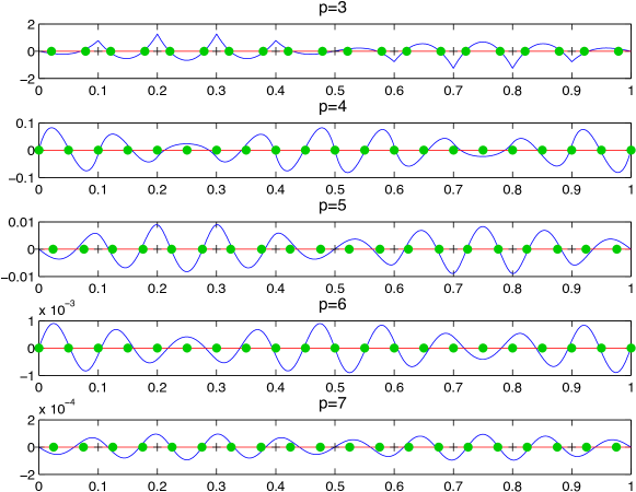
Figure 5: Residuals of periodic problem with 10 elements.

For easiness of exposition, from now on we refer to the “surrogate” superconvergent points simply as superconvergent points, although this might not be technically true.

For multi-dimensional problems on a NURBS single-patch geometry, the superconvergent points can be obtained by further mapping the tensor product of one-dimensional superconvergent points through the geometry map $\mathbf{F}$ in the physical domain. Clearly, the same considerations of the one-dimensional case are valid.

3.4 Least-Squares at Superconvergent Points (LS-SP)

As already mentioned, the Least-Squares at Superconvergent Points method (LS-SP) has been introduced by [1]. In this method all the superconvergent points are used as collocation points. As it can be seen in Table 2, there are at least two superconvergent points per element; if we take all of them as collocation points, we obtain an overdetermined system of equations if the number of elements is large enough: such linear system is then solved in a least-squares sense, leading to a method which is not strictly a collocation method. The order of convergence of the method as measured in numerical tests is reported in Table 1: note that it is optimal for odd degrees and one-order sub-optimal in $L^{2}$ for even degrees, while it is optimal regardless of the parity of $p$ in $H^{1}$ and $H^{2}$ norm.

Figure 6 shows the superconvergent points for $p=3,\ldots,7$ on a knot vector with 10 elements. Observe that the same least-squares formulation can accommodate for both Dirichlet problems (i.e., open knot vectors) and periodic problems.

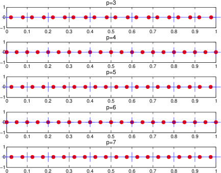
Figure 6: Superconvergent points for $p=3,\ldots,7$ on a knot vector with 10 elements.

3.5 Collocation at Alternating Superconvergent Points (C-ASP)

C-ASP is a collocation method introduced in [2]. In this method, a subset of superconvergent points with cardinality equal to the number of degrees-of-freedom is employed as set of collocation points. The authors of [2] select a subset of the superconvergent points in such a way that every element of the knot span contains at least one collocation point; note that this roughly means considering every other superconvergent point, hence the name we give to the method. Because we need to select as many collocation points as degrees of freedom, the easiest case is when one considers the periodic Problem 2, for which the number of elements is identical to the number of degrees-of-freedom, so that exactly one superconvergent point per element is selected, see Figure 7 (this case is not considered in [2]). Note that for even $p$ one possibility is then to select the midpoint of each element, i.e., the Greville points for the uniform knot vector, see Figure LABEL:aspperiodiceven. For the Dirichlet Problem 1, one needs instead to select $n_{el}+p-2$ collocation points on a mesh of $n_{el}$ elements. To this end, an ad-hoc algorithm is presented in [2] that selects suitable superconvergence points in the internal part of the domain, and “blends them” with Greville points on the elements close to the boundary, as can be seen in Figure 8. Note that other choices for the elements close to the boundary can be envisaged, which however do not affect the convergence order of the method, see [28].

(a)

(b)

Figure 7: Example of C-ASP points for the periodic Problem 2. The collocation points are marked with full red dots, while the remaining superconvergent points are displayed with green circles. In this case, C-ASP and C-GP coincide for even degrees.

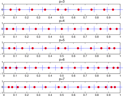
Figure 8: Example of C-ASP points for the Dirichlet problem 1 over a knot vector with 9 elements. The points adjacent to the boundary are obtained according to Algorithm 1 of [2].

The convergence orders of C-ASP assessed numerically by [2] are also reported in Table 1. Note in particular that the $L^{2}$ order of convergence for C-ASP is $p$ regardless of the parity of $p$, i.e., one-order suboptimal, while the $H^{1}$ and $H^{2}$ orders of convergence are optimal, again regardless of the parity of $p$.

3.6 Collocation on Clustered Superconvergent Points (C-CSP)

We now describe a new choice of collocation points among the superconvergent points, alternative to C-ASP, which we name Collocation on Clustered Superconvergent Points (C-CSP).

To understand our approach, we describe it first in the simplest setting, i.e., the periodic Problem 2 with even number of elements and odd degree $p$. We look for a periodic distribution of collocation points which is furthermore symmetric at the element scale. This can be achieved by selecting two superconvergent points in an element and then skipping the following one, as depicted in Figure 9. Surprisingly, the order of convergence of C-CSP in this case is optimal, cf. the numerical results in Section 4, Figure 14. For even degrees, we have experimented different selections of sets of superconvergent points, preserving periodicity and some local symmetry, two of which are depicted in Figure 10 (observe that with the first one we end up with Greville points again). In all cases, we have measured numerically one-order suboptimal convergence in $L^{2}$, i.e., we do not see improvements with respect to C-GP, LS-SP or C-ASP, see the numerical results in Section 4, Figure 15. At this point, only the odd-degree C-CSP seems to deserve further interest, and we will restrict to this case in the remaining of the paper. How to use efficiently the superconvergent points in an even degree splines collocation scheme remains an open problem.

The next step is to extend (odd-degree) C-CSP to the open knot vector to solve the Dirichlet Problem 1. To this end, we need to include additional points, which are taken among the other superconvergent points populating the elements close to the boundary, and trying to preserve symmetry, see Figures 11 and 12. Note that when the number of elements is even the procedure just described will not yield a globally symmetric distribution of collocation points, cf. Figure 12. We can however restore symmetry with a little modification of the collocation approach: we add one (or a few) points to the collocation set to restore symmetry of the collocation scheme, and average the equations corresponding to the points located at the center of the domain in order to match the number of unknown. This procedure is depicted in Figure 13 for $p=3$.

The order of convergence of C-CSP on regular meshes, reported in Table 1, is the same of LS-SP, i.e., optimal for odd degrees. As already mentioned, all our attempts to extend it to even degree splines has produced one order suboptimal convergence. These convergence rates have been measured by running the numerical benchmarks detailed in Section 4, also covering the symmetric variant of Figure 12.

Figure 9: Periodic C-CSP stencil for odd degree: the collocation points are marked with full red dots, while the remaining superconvergent points are displayed with green circles.

Figure 10: Attempts of C-CSP stencil for even degree: the collocation points are marked with full red dots, while the remaining superconvergent points are displayed with green circles. The construction at the top leads to Greville points, while the one at the bottom yields symmetry at a macro-element level.

Figure 11: C-CSP points for a Dirichlet problem solved on a mesh with 9 elements (odd number of elements, leading to a symmetric set of point): the collocation points are marked with full red dots, while the remaining superconvergent points are displayed with green circles. Black dots represent the points added with respect to the periodic stencil.

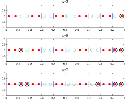
Figure 12: C-CSP points for a Dirichlet problem solved on a mesh with 10 elements (even number of elements, leading to a non-symmetric set of point): the collocation points are marked with full red dots, while the remaining superconvergent points are displayed with green circles. Black dots represent the points added with respect to the periodic stencil.

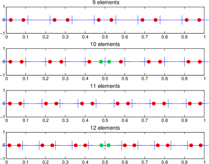
Figure 13: C-CSP symmetric-variant points for a Dirichlet problem with $p=3$: the collocation points are marked with red dots, while the superconvergent points whose equations have to be averaged are displayed with green dots.

4 Numerical tests

This section is devoted to the numerical benchmarking of the new C-CSP method, and its comparison to the other approaches recalled in Section 3. For conciseness, we do not show convergence results in $L^{\infty}$ norm, which we found to be identical to the ones in $L^{2}$ norm in each of the tests reported below, see [28].

We begin by testing C-CSP on the periodic Problem 2, with $a_{0}=a_{1}=1$ and with $f(x)=(1+4\pi^{2})\sin(2\pi x)+2\pi\cos(2\pi x)$, whose solution is $u(x)=\sin(2\pi x)$. As previously discussed, this is the only test for which we present results for even degrees $p$: we see from the plots in Figures 14 and 15 that the orders of convergence for the $L^{2}$ norm of the error are optimal, i.e. equal to $p+1$, for odd values of $p$, while for even $p$ the measured convergence rate is only $p$, i.e. one-order suboptimal.

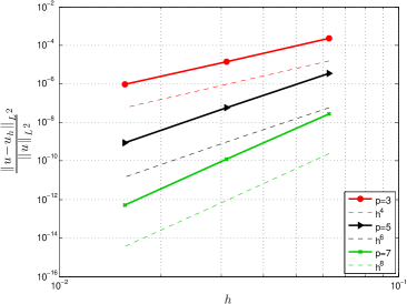
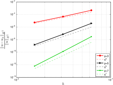
Figure 14: $L^{2}$ and $H^{1}$ error plot: C-CSP periodic problem (odd $p$).

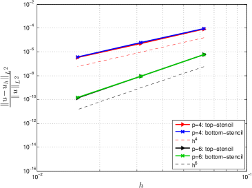
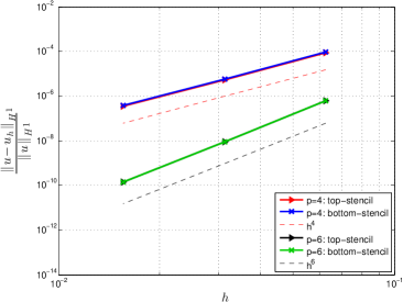
Figure 15: $L^{2}$ and $H^{1}$ error plot for C-CSP periodic problem (even $p$), with the stencils depicted in Figure 10.

A natural question arises: why can’t we achieve optimal convergence when even degrees B-splines are considered? The answer is not yet clear. As we explained in the previous sections, the rationale behind C-CSP, as well as LS-SP and C-ASP, is to try to obtain the same solution delivered by the Galerkin method by imposing the residual to be zero at the superconvergent points, which are supposedly close to the true zeros of the Galerkin residual. However, as we discussed in Section 3.3, we do not have access to the precise location of the superconvergent points, and instead we use “surrogate” superconvergent points that do not approximate well the zeros of the Galerkin residual everywhere in the domain. We do not see however any qualitative difference between the odd and even case other than in the central element (although we did not perform a quantitative analysis of this issue). Furthermore, it is not clear why the C-ASP points would have poorer approximation properties than the C-CSP ones: in other words, the points that would be selected by the C-ASP seem as good as those that would be selected by the C-CSP as for what concerns being close to the zeros of the Galerkin residual. It could be that the local symmetry of the C-CSP points distribution leads to some error cancellation in the collocation system.

We continue by testing the C-CSP method on the Dirichlet Problem 1 with $a_{0}=a_{1}=0$ and $f(x)=\pi^{2}\sin(\pi x)$, whose exact solution is $u(x)=\sin(\pi x)$, and show the corresponding results in Figure 16. As in the previous case, the order of convergence is $p+1$ in $L^{2}$ norm and $p$ in $H^{1}$ norm. In order to compare the four methods we presented (C-CSP, ASP, LS-SP and Greville collocation) against the Galerkin solver, we show in Figure 17 a comparison of the convergence of the $L^{2}$-error obtained when solving the Dirichlet problem above with B-splines of degree $p=3$. The plot highlights that C-CSP, although converging with optimal order, shows an error one order of magnitude larger than Galerkin, while LS-SP converges essentially to the same solution of the Galerkin method. It should be observed however that the computational cost of LS-SP is significantly higher than C-CSP, not only because of the number of points where the residual needs to be evaluated (about $2^{d}$ times more that C-CSP in $d$ dimensions) but also for the the higher condition number of the resulting system of linear equations.

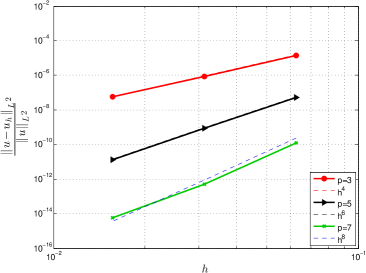
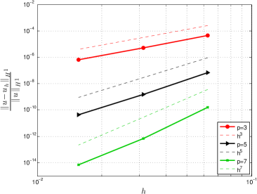
Figure 16: $L^{2}$ and $H^{1}$ error plot: C-CSP Dirichlet problem.

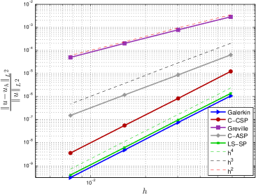
Figure 17: Comparison of convergence of $L^{2}$ error norms for the Dirichlet problem for different methods.

We also investigate the robustness of the method with respect to perturbations of the knot vector. To this end, we perturb the internal knots of each equispaced open knot vector considered in the convergence analysis by randomly chosen quantities, i.e. we replace each internal knot $\xi_{i}$ by $\tilde{\xi}_{i}=\xi_{i}+\frac{1}{10n_{el}}X_{i}$, where $X_{i}$ are independent random numbers $X_{i}\in[-1,1]$. We remark that the random quantities $X_{i}$ are generated at every refinement step for each node of the knot vector. The scaling factor $\frac{1}{10n_{el}}$ prevents knot clashes and furthemore the resulting knot vectors are quasi-uniform, but the local symmetry of the mesh is lost for all elements of the mesh. This is expected to have an influence on the location of the superconvergent points, but we nonetheless select the collocation points following the element-wise construction for the uniform mesh case. The error plots are shown in Figures LABEL:fig:rand.knots.L2 and LABEL:fig:rand.knots.H1. We note that we loose the optimal rates of convergence we observed in the previous tests: the order of convergence is $p$ for both the $L^{2}$ and $H^{1}$ error norm, i.e., optimal for the $H^{1}$ error norm and only one-order suboptimal for the $L^{2}$ one.

We also verify the influence of the differential operator and of the boundary conditions, by considering non-null $a_{0}$ and $a_{1}$ in the Dirichlet Problem 1, as well as Neumann-Neumann and Neumann-Dirichlet boundary conditions. We performed several tests and the results obtained were identical; therefore, we report here only one representative example, see [28] for additional numerical results. In detail, we consider $a_{1}(x)=x$, $a_{0}=1$ and $f(x)=x(e^{x}\sin(\pi x)+\pi e^{x}\cos(\pi x))-2\pi e^{x}\cos(\pi x)+\pi^{2}e^{x}\sin(\pi x)$, whose exact solution is $u(x)=\sin(\pi x)e^{x}$. The results of the test we performed are shown in Figures LABEL:fig:adv.reac:L2 and LABEL:fig:adv.reac:H1: the order of convergence is still optimal: $p+1$ for the $L^{2}$ error norm, and $p$ for the $H^{1}$ norm. We can then conclude that the C-CSP method seems to be robust with respect the form of the elliptic operator.

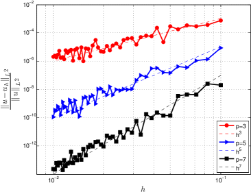
(a)

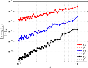
(b)

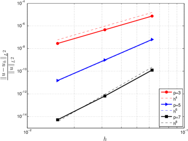
(c)

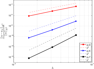
(d)

Figure 18: Robustness test for C-CSP with respect to perturbation of the knot vectors (plots LABEL:fig:rand.knots.L2 and LABEL:fig:rand.knots.H1) and changes of the differential operator (plots LABEL:fig:adv.reac:L2 and LABEL:fig:adv.reac:H1).

Finally, we present two examples of two-dimensional Dirichlet Problem 3 solved by C-CSP. In the first one we consider as computational domain, $\Omega$, the quarter of annulus in Figure LABEL:ring (for which NURBS functions have to be employed), and $f(x,y)$ is chosen such that the exact solution is $u(x,y)=-(x^{2}+y^{2}-1)(x^{2}+y^{2}-4)xy^{2}$. In Figures LABEL:2Dringcspall:p3, LABEL:2Dringcspall:p5 and LABEL:2Dringcspall:p7 we show the convergence plots of the $L^{2}$ and $H^{1}$ errors for the C-CSP and Galerkin methods for odd degree NURBS $p=3,5,7$. The observed orders of convergence are as expected: optimal order in $L^{2}$ norm and $H^{1}$ norm. We remark that for $p=3$ the $H^{1}$ norms of the corresponding errors obtained by the Galerkin and C-CSP methods are very close, as can be seen in Figure LABEL:2Dringcspall:p3.

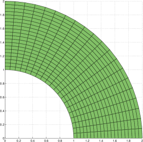
(a)

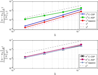
(b)

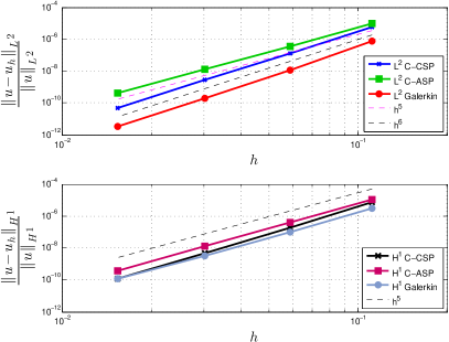
(c)

(d)

Figure 19: Ring domain and $L^{2}$ and $H^{1}$ convergence of approximations with $p=3,5,7$.

In the second two-dimensional example, we let $\Omega$ be the rhombus with vertices $(0,0)$, $(\frac{1}{4},1)$, $(1,\frac{1}{4})$ and $(\frac{5}{4},\frac{5}{4})$, represented in Figure LABEL:rhombus (its parametrization is bilinear but not orthogonal, as in the previous example), and $f$ is such that the exact solution is $u(x,y)=\sin\left(\frac{4}{15}\pi(y-4x)\right)\sin\left(\frac{16}{15}\pi\left(\frac{x}{4}-y\right)\right)(x^{3}+y^{3})$. The corresponding errors are shown in Figures LABEL:2Drhombusall:p3, LABEL:2Drhombusall:p5 and LABEL:2Drhombusall:p7, and the same observations as before hold. Note however that the gap between the C-CSP and the Galerkin solution is larger than in the previous example, especially for the $L^{2}$ error. Moreover, for $p=5$ and $p=7$ the convergence is still in its preasymptotic regime.

(a)

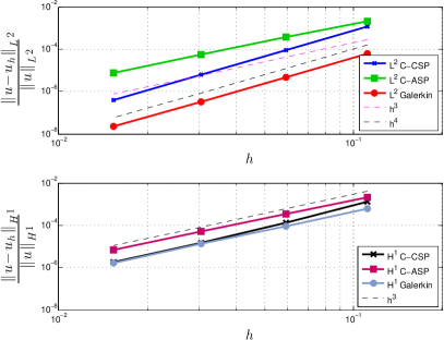
(b)

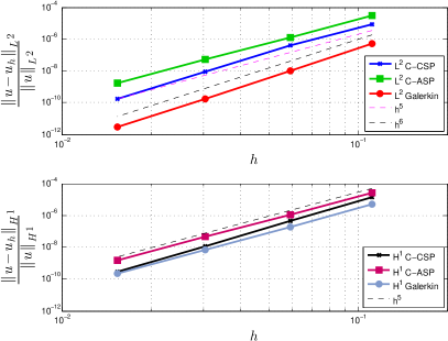
(c)

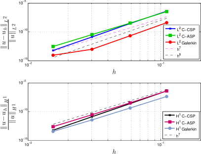
(d)

Figure 20: Rhombus domain and $L^{2}$ and $H^{1}$ convergence of approximations with $p=3,5,7$.

5 Conclusion

In this paper we have proposed an isogeometric collocation method based on the superconvergent Galerkin points, in the framework of [2]. Our guiding criterion for the subset of the superconvergent points is however different, and consists in picking up clusters of points, in such a way to obtain a collocation scheme symmetric at element-scale. This choice allows to recover optimal convergence rates for odd-degrees splines/NURBS, without “oversampling” the domain as in least-square approach proposed by [1]. Moreover, the order of convergence of the $L^{\infty}$ norm of the error is the same of $L^{2}$-norm in all experiments we have performed (not shown in the paper for the sake of brevity).

The preliminary numerical campaign on one- and two-dimensional tests that we performed suggests that the method is robust with respect to isogeometric mapping of the domain, while perturbations of the knot vector may reduce the accuracy of the method. A rigorous mathematical explanation for the convergence behavior observed for the proposed method, and for the other collocation methods based on the Galerkin superconvergent points, is not available yet and will be the target of our future efforts.

References

- [1] C. Anitescu, Y. Jia, Y. J. Zhang, T. Rabczuk, An isogeometric collocation method using superconvergent points, Computer Methods in Applied Mechanics and Engineering 284 (2015) 1073–1097.
- [2] H. Gomez, L. De Lorenzis, The variational collocation method, Computer Methods in Applied Mechanics and Engineering 309 (2016) 152–181.
- [3] W. Bickley, Piecewise cubic interpolation and two-point boundary problems, The computer journal 11 (2) (1968) 206–208.
- [4] D. Fyfe, The use of cubic splines in the solution of two-point boundary value problems, The computer journal 12 (2) (1969) 188–192.
- [5] E. N. Houstis, E. Vavalis, J. R. Rice, Convergence of cubic spline collocation methods for elliptic partial differential equations, SIAM Journal on Numerical Analysis 25 (1) (1988) 54–74.
- [6] R. D. Russell, L. F. Shampine, A collocation method for boundary value problems, Numerische Mathematik 19 (1) (1972) 1–28.
- [7] C. De Boor, B. Swartz, Collocation at gaussian points, SIAM Journal on Numerical Analysis 10 (4) (1973) 582–606.
- [8] D. N. Arnold, W. L. Wendland, The convergence of spline collocation for strongly elliptic equations on curves, Numerische Mathematik 47 (3) (1985) 317–341.
- [9] T. J. R. Hughes, J. A. Cottrell, Y. Bazilevs, Isogeometric analysis: CAD, finite elements, NURBS, exact geometry and mesh refinement, Comput. Methods Appl. Mech. Engrg. 194 (39) (2005) 4135–4195.
- [10] J. A. Cottrell, T. J. R. Hughes, Y. Bazilevs, Isogeometric Analysis: toward integration of CAD and FEA, John Wiley & Sons, 2009.
- [11] F. Auricchio, L. Beirão da Veiga, T. Hughes, A. Reali, G. Sangalli, Isogeometric collocation methods, Mathematical Models and Methods in Applied Sciences 20 (11) (2010) 2075–2107.
- [12] F. Auricchio, L. Beirão da Veiga, J. Kiendl, C. Lovadina, A. Reali, Locking-free isogeometric collocation methods for spatial Timoshenko rods, Comput. Methods Appl. Mech. Engrg. 263 (2013) 113 – 126.
- [13] F. Auricchio, L. Beirão da Veiga, T. J. R. Hughes, A. Reali, G. Sangalli, Isogeometric collocation for elastostatics and explicit dynamics, Comput. Meth. Appl. Mech. Engrg. 249–252 (2012) 2–14.
- [14] L. Beirao da Veiga, C. Lovadina, A. Reali, Avoiding shear locking for the Timoshenko beam problem via isogeometric collocation methods, Computer Methods in Applied Mechanics and Engineering 241 (2012) 38–51.
- [15] J. Kiendl, F. Auricchio, L. Beirao da Veiga, C. Lovadina, A. Reali, Isogeometric collocation methods for the reissner–mindlin plate problem, Computer Methods in Applied Mechanics and Engineering 284 (2015) 489–507.
- [16] A. Reali, H. Gomez, An isogeometric collocation approach for Bernoulli–Euler beams and Kirchhoff plates, Computer Methods in Applied Mechanics and Engineering 284 (2015) 623–636.
- [17] L. De Lorenzis, J. Evans, T. Hughes, A. Reali, Isogeometric collocation: Neumann boundary conditions and contact, Computer Methods in Applied Mechanics and Engineering 284 (2015) 21–54.
- [18] A. Reali, T. J. Hughes, An introduction to isogeometric collocation methods, in: Isogeometric Methods for Numerical Simulation, Springer, 2015, pp. 173–204.
- [19] H. Casquero, L. Liu, Y. Zhang, A. Reali, H. Gomez, Isogeometric collocation using analysis-suitable T-splines of arbitrary degree, Computer Methods in Applied Mechanics and Engineering 301 (2016) 164–186.
- [20] M. Matzen, T. Cichosz, M. Bischoff, A point to segment contact formulation for isogeometric, NURBS based finite elements, Computer Methods in Applied Mechanics and Engineering 255 (2013) 27–39.
- [21] H. Gomez, A. Reali, G. Sangalli, Accurate, efficient, and (iso) geometrically flexible collocation methods for phase-field models, Journal of Computational Physics 262 (2014) 153–171.
- [22] C. Manni, A. Reali, H. Speleers, Isogeometric collocation methods with generalized B-splines, Computers & Mathematics with Applications 70 (7) (2015) 1659–1675.
- [23] D. Schillinger, J. A. Evans, A. Reali, M. Scott, T. Hughes, Isogeometric collocation: Cost comparison with Galerkin methods and extension to adaptive hierarchical NURBS discretizations, Computer Methods in Applied Mechanics and Engineering 267 (2013) 170–232.
- [24] F. Calabrò, G. Sangalli, M. Tani, Fast formation of isogeometric Galerkin matrices by weighted quadrature, arXiv preprint arXiv:1605.01238.
- [25] C. de Boor, A practical guide to splines, revised Edition, Vol. 27 of Applied Mathematical Sciences, Springer-Verlag, New York, 2001.
- [26] L. Piegl, W. Tiller, The NURBS book, Springer, 2012.
- [27] L. B. Wahlbin, Superconvergence in Galerkin finite element methods, Springer, 1995.
- [28] M. Montardini, A new isogeometric collocation method based on galerkin superconvergent points, Master’s Thesis, Università di Pavia (2016).