Infrared optical properties of $\alpha$ quartz by molecular dynamics simulations

Abstract

This paper is concerned with theoretical estimates of the refractive–index curves for quartz, obtained by the Kubo formulæ in the classical approximation, through MD simulations for the motions of the ions. Two objectives are considered. The first one is to understand the role of nonlinearities in situations where they are very large, as at the $\alpha$–$\beta$ structural phase transition. We show that on the one hand they don’t play an essential role in connection with the form of the spectra in the infrared. On the other hand they play an essential role in introducing a chaoticity which involves a definite normal mode. This might explain why that mode is Raman active in the $\alpha$ phase, but not in the $\beta$ phase. The second objective concerns whether it is possible in a microscopic model to obtain normal mode frequencies, or peak frequencies in the optical spectra, that are in good agreement with the experimental data for quartz. Notwithstanding a lot of effort, we were unable to find results agreeing better than about 6%, as apparently also occurs in the whole available literature. We interpret this fact as indicating that some essential qualitative feature is lacking in all models which consider, as the present one, only short–range repulsive potentials and unretarded long–range electric forces.

PACS: 78.20.Ci, 42.70.Ce, 63.20.Ry

1 Introduction

A subject of great current interest is that of a microscopic description of the ferroelectric transition. It is known that at the transition a divergence of the dielectric constant $\varepsilon(\omega)$ at $\omega=0$ occurs, which in most cases is understood as corresponding to the fact that the frequency of an infrared peak goes to zero. On the other hand, the infrared frequencies are usually studied via a linear analysis of phonon dispersion relations, while the nonlinear contribution to the dynamics should be relevant at the transition to the ferroelectric phase, as should be near any phase transition. So the problem arises of how the infrared peaks should be described in a fully nonlinear setting. A description can actually be given through the study of the time autocorrelation of the polarization due to the ions, which can be computed in the classical approximation via molecular dynamics simulations. Computations of this type were indeed performed successfully in the case of LiF [1], with results that agree with the experimental data in a surprisingly good way.

At the moment, as will be explained below, we are unable to study ferroelectrics through molecular dynamics. So in this paper we limit ourselves to quartz, which is not a ferroelectric material, but however presents a divergence in the dielectric constant at the temperature of the $\alpha$–$\beta$ transition. We compute here its refractive index curves in the infrared region. Our main concerns are the dynamical properties of the system, particularly at the $\alpha$–$\beta$ transition, and the quantitative agreement between calculated and experimental spectra in the infrared for $\alpha$ quartz.

As is well known [2], linear analysis shows that quartz is doubly refractive and that the peaks in its refractive–index curves correspond to the frequencies of the active normal modes. Such qualitative results are confirmed by the present molecular dynamics simulations for $\alpha$ quartz at high temperatures, even at the transition to the $\beta$ phase, notwithstanding the high nonlinearity of the system. This quantitative agreement of the nonlinear results with those of the linear analysis, in particular for the values of the frequencies, is quite surprising, in view of the large nonlinear contributions, and probably is due to some deep reason not yet fully understood. On the other hand, both the linear analysis and our nonlinear study fail in perfectly reproducing the experimental data, as some systematic deviations are observed. We tried several procedures for choosing the parameters, both of the linear model and of the nonlinear one, in order to find a better agreement with the experimental curves. But there was no way of reducing the relative error below a threshold of the order of 6%. This fact, too, requires an explanation. These are the two main results of the present work.

2 The model

Figure 1: Refractive index (real part) versus $\omega$ for the ordinary ray, at temperatures $T=1\,$K (red line) and $T=300\,$K (dark line). Color online.

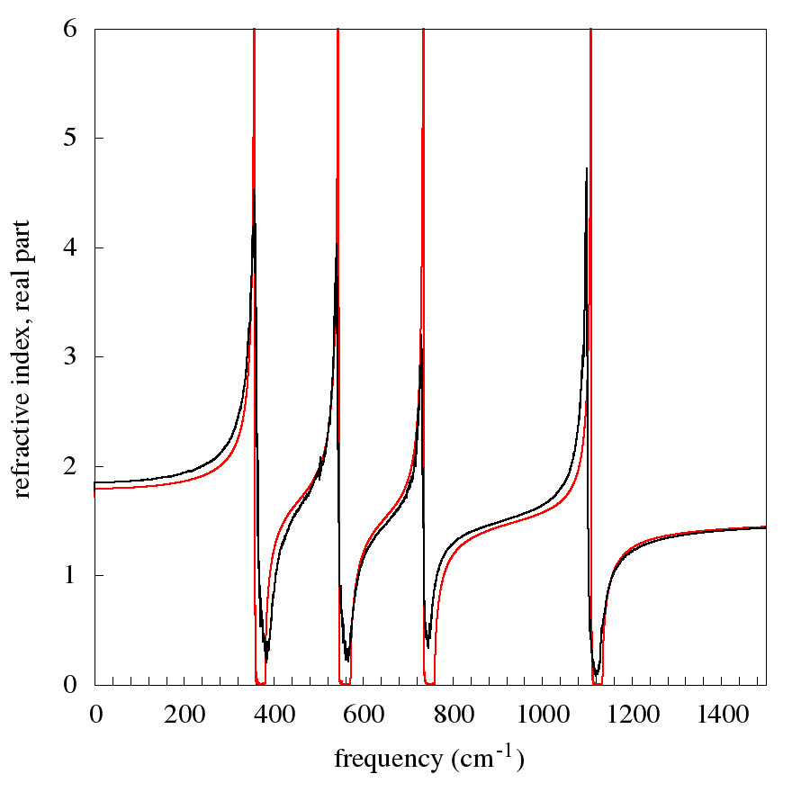
Figure 2: Same as Figure 1 for the extraordinary ray.

		$\alpha$ quartz parameters
	$a$	$b$	$c$
	4.9137 Å	4.9137 Å	5.4047 Å
	$x$	$y$	$z$
Si	0.4697	0.0000	0.0000
O	0.4133	0.2672	0.1188
		$\beta$ quartz parameters
	$a$	$b$	$c$
	4.9965 Å	4.9965 Å	5.4546 Å
	$x$	$y$	$z$
Si	0.5000	0.0000	0.0000
O	0.4157	0.2078	0.1667

Table 1: Geometric parameters for $\alpha$ and $\beta$ quartz (see text).

It is known that the primitive cell of quartz contains nine atoms (three silicon and six oxygen atoms). Moreover, it has the form of a right prism of rhomboidal basis, corresponding to three basis vectors ${\bf a},{\bf b},{\bf c}$ with ${\bf a}$ and ${\bf b}$ forming an angle of 120^∘ and ${\bf c}$ orthogonal to ${\bf a}$ and ${\bf b}$. In Table 1 we report the lengths of the three basis vectors at normal conditions of temperature and pressure ($300\,\mathrm{K}$ and 1 bar), as given by [3], which we use in our simulations. We also report the fractional coordinates $x$,$y$,$z$ (along the three basis vectors) of a silicon atom and of an oxygen atom, out of which all other coordinates can be generated by symmetry transformations. The configuration corresponding to $\alpha$ quartz is thought of as being the more stable equilibrium configuration of the system. In order to simulate the crystal, we choose a domain $D\subset\mathbb{R}^{3}$ (fundamental box) constituted by $4\times 4\times 4$ primitive cells, with a number $N=9\times 4^{3}=576$ of point particles inside it. Due to the partially ionic character of the quartz crystal, the point particles have to be endowed with suitable effective charges, $e_{S}$ for the silicon ion and $e_{O}$ for the oxygen ion, with the neutrality constraint

$$2e_{O}+e_{S}=0\ .$$ (1)

Thus, Coulomb long range forces come into play and, in order to take them into account, working however with a small number $N$ of particles, periodic boundary conditions are imposed. In addition to the electric forces, short-range two-body spherically symmetric potentials are introduced, one for each of the pairs Si-Si, O-O, Si-O. These potentials are taken of a form which is extensively used for quartz, namely (see [4, 5]),

$$U(r)=Ae^{-Br}-\frac{C}{r^{6}}\ ,$$ (2)

($r$ being the interatomic distance), with a triple of parameters $A$, $B$, $C$ a priori different for each pair. In the numerical calculations, for the short-range interactions a cutoff of 9 Å was imposed, while the Coulomb interactions were dealt with through standard Ewald summations. This is exactly the point where some modifications are required if one aims at dealing with ferroelectrics. Indeed the Ewald resummation provides a periodic electric field having a vanishing mean, at variance with what occurs with ferroelectrics. The problem of how to modify accordingly the Ewald procedure is left for a possible future work.

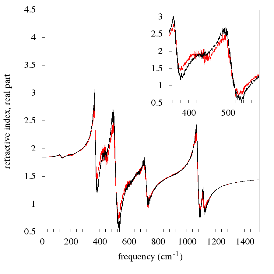
Figure 3: Refractive index (real part) versus $\omega$ for the ordinary ray, at temperature $T=670\,$K, below the phase transition (red line), and at $T=700\,$K, above it (dark line). The inset exhibits the new peak at about 455 cm^-1 in the $\beta$ phase. Color online.

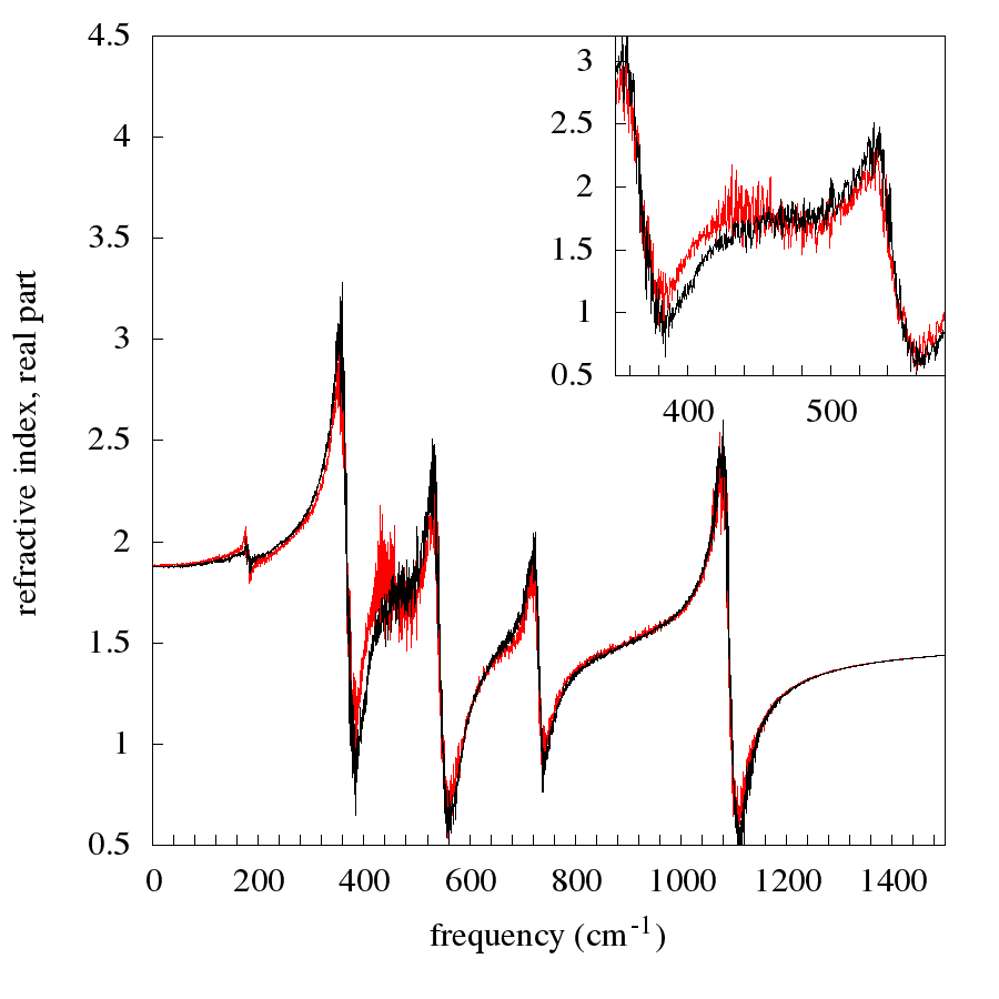
Figure 4: Same as Figure 3 for the extraordinary ray.

The masses are taken from the literature, so that to fix the model there remains a total of 10 free parameters: one effective charge (for example that of oxygen) and the three parameters $A$, $B$, $C$ of the short-range potential for each of the three pairs Si-O, O-O, Si-Si. The values of the potential parameters adopted are reported in Table 2, while we used the values $e_{S}=2.04191$ and $e_{O}=-1.02096$ for the effective charge (in unit of electron charge) of Si and O respectively. They were determined by optimization procedures aimed at obtaining the best possible agreement between the computed refractive index curves and the empirical ones at 300 K, requiring in addition that the $\alpha$ structure be stable at that temperature and at larger (but not too much) temperatures. With the values thus determined for the parameters of the model it turns out, as will be shown below, that the $\alpha$–$\beta$ transition occurs at a temperature of about $T=700\,$K, which is a rather low value. We leave for a future work the task of performing an optimization of the parameters with a procedure which takes both the frequencies and the transition temperature into account.

	$A$ (eV)	$B$ (Å${}^{-1})$	$C$ (eV Å${}^{6})$
Si-O	18207.1	4.88538	135.021
O-O	501.814	2.76745	15.0427
Si-Si	25.3672	1.41444	0.694560

Table 2: Parameters of the short range potential.

The equations of motion were numerically solved using a Verlet algorithm, with integration step of 2 fs, at several values of temperature. Having chosen to work in a purely Hamiltonian frame, temperature was determined through the choice of the initial data. In principle this should be obtained by extracting the data according to a Gibbs distribution. This being impracticable, we followed the alternative standard procedure. Namely, one puts the particles at the $\alpha$ equilibrium point, while their velocities are extracted from a Maxwell–Boltzmann distribution at a suitable temperature. Then one lets the system thermalize, which usually takes a time of the order of 2 ps (1000 integration steps), and temperature is eventually identified through the mean kinetic energy of the ions. Then one starts computing means and correlations of the relevant quantities.

3 The refractive–index curves

The refractive index is obtained by computing the electric permittivity tensor $\varepsilon_{ij}(\omega)$ as a function of frequency, and diagonalizing it at each given frequency. As expected, two eigenvalues are found to coincide, and the square root of such a value is precisely the refractive index of the ordinary ray. The refractive index of the extraordinary ray is instead the square root of the remaining eigenvalue.

The connection with dynamics is obtained through the susceptibility tensor $\chi_{ij}(\omega)$ due to the ions, which is related to permittivity by

$$\varepsilon_{ij}(\omega)=\delta_{ij}+4\pi(\chi_{ij}\left(\omega)+\chi^{el}_{ij}\right)\ .$$ (3)

Here, $\chi^{el}$ is the contribution of the electrons, which turns out to be constant in the infrared domain (see [6]). Instead, the ions’ contribution $\chi_{ij}(\omega)$ is obtained numerically according to Green-Kubo linear response theory (see for example [7]) as follows. One considers the polarization $\mathbf{P}$, which is defined in microscopic terms as

$$\mathbf{P}=\frac{1}{V}\sum_{l}e_{l}\mathbf{x}_{l}\ ,$$ (4)

where $V$ is the volume of the simulation domain (or fundamental box), while $\mathbf{x}_{l}$ is the position vector of the $l$–th ion, of charge $e_{l}$.

Then at temperature $T$ one has

$$\chi_{ij}(\omega)=\frac{V}{k_{B}T}\int_{0}^{+\infty}e^{-i\omega t}\langle P_{i}(t)\dot{P}_{j}(0)\rangle dt\ ,$$ (5)

$k_{B}$ being the Boltzmann constant. Here $\langle\cdot\rangle$ should in principle be the canonical average. Actually the averages were estimated as the mean of the time averages calculated along a certain number (usually 40) of different MD trajectories, calculated for 200 ps.

A first set of results is illustrated in Figures 1 and 2. In the first figure we report, vs frequency, the real part of the refractive index for the ordinary ray at $T=300\,\mathrm{K}$ (dark line) and at $T=1\;\mathrm{K}$ (red line). The analogous spectra for the extraordinary ray are reported in Figure 2. At a temperature as low as $T=1\;\mathrm{K}$ the spectrum is determined essentially by the linear approximation, so that the peaks correspond to the frequencies of the normal modes (actually, those of the so called type $A_{2}$ and $E$; see [2]). The results show that the spectrum at $T=300\,\mathrm{K}$ does not differ essentially from that corresponding to $1\;\mathrm{K}$, apart from a consistent broadening of the peaks and some small shifts in their frequencies.

A second set of results concerns the behavior of the spectra at the structural $\alpha$–$\beta$ phase transition which, in the present microscopic model, with the choice made for the parameters, turns out to occur in a region of temperatures roughly around $T=690\,$K. This will be shown in a moment. So we computed the refractive–index curves at $T=670\,$K, an $T=700\,$K, which are reported in Figure 3 for the ordinary ray and in Figure 4 for the extraordinary ray.

The figures show that, at the transition, the optical spectra are still dominated by the linear behavior. Indeed, in both figures the two curves relative to the two temperatures essentially superpose one another, and one can notice the same peaks of the previous Figures 1 e 2, just a little more broadened and noisy.

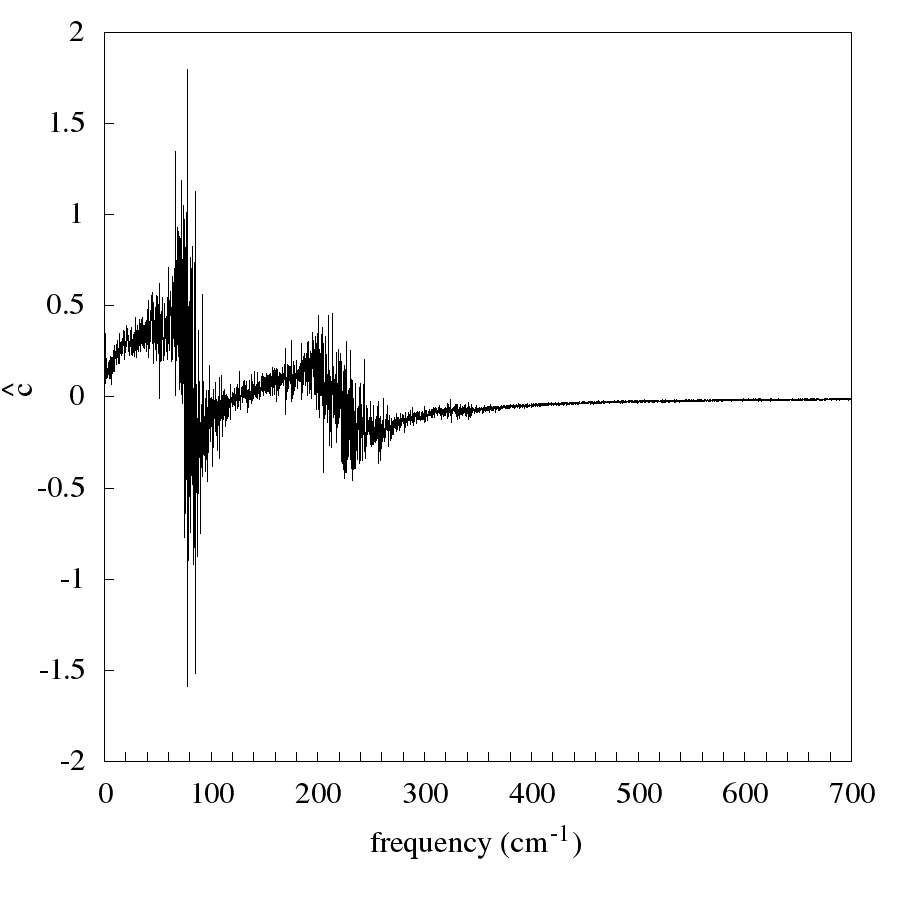
Figure 5: Fourier transform $\hat{C}$ of the time–autocorrelation of the amplitude of the mode $\omega=232$ cm^-1, at temperature $T=690\,\mathrm{K}$.

Some differences however show up. The most important one is the appearance of one more peak (see the inset) in the $\beta$ phase at $\omega\simeq 455$ cm^-1, that should correspond to a normal mode which is only Raman active in the $\alpha$ phase. In addition, a small peak appears at approximately 200 cm^-1 in the extraordinary ray, which should presumably be due to the nonlinearity.

So the harmonic approximation essentially still dominates up to the transition temperature, at least for what concerns the refractive index. On the other hand the transition has a relevant effect on at least one of the normal modes of the system, the one corresponding to the normal mode frequency $\omega=206$ cm^-1 (not active in the infrared) which, with the choice made for the parameters of our model, occurs at about $\omega=232$ cm^-1. Indeed such a mode exhibits a chaotic behavior precisely at the transition. This can be seen from Figure 5, where the Fourier transform $\hat{C}$ of the time–autocorrelation of the mode amplitude at temperature 690 K is reported vs frequency. One sees that the peak in question disappears, being replaced by a very complex structure, characteristic of a chaotic motion. This fact might entail an effect on the Raman spectrum. Indeed the mode in question is known to be Raman active in the $\alpha$ quartz but not in the $\beta$ quartz, and this seems to be explained by the chaoticity exhibited here at the transition. We leave for future work a detailed analysis of the behavior of the normal modes at the transition.

4 The $\alpha$–$\beta$ transition

The occurrence of the transition is exhibited in terms of an “order parameter”, which discriminates between the configurations of the two phases. Following essentially [8] and [9], we define it as follows.

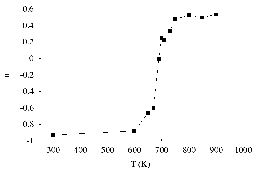
Figure 6: The order parameter $u$ (see eq. 6) as a function of $T$. A negative value corresponds to the $\alpha$ quartz phase, while a positive value corresponds to the $\beta$ quartz phase. A rather abrupt change is exhibited near $T\simeq 690\,$K.

Consider the representative position vectors of silicon and of oxygen, defined through their mean fractional coordinates (i.e., as the averages, over the elementary cells, of the fractional coordinates of such atoms). Consider also their time averages (actually a mean of such averages, taken over several independent simulations), which we denote by $\mathbf{x}_{S}$, $\mathbf{x}_{O}$. Then consider the position vectors $\mathbf{x}^{\alpha}_{S}$ and $\mathbf{x}^{\alpha}_{O}$, defined by the experimental fractional coordinates of silicon and of oxygen for $\alpha$ quartz, taken from Table 1. Analogously define $\mathbf{x}^{\beta}_{S}$ and $\mathbf{x}^{\beta}_{O}$.

Thus the distance $d_{\alpha}$ of the mean configuration of the system from the equilibrium $\alpha$ configuration is naturally estimated as

$$d_{\alpha}=\sqrt{\|\mathbf{x}_{S}-\mathbf{x}^{\alpha}_{S}\|^{2}+\|\mathbf{x}_{O}-\mathbf{x}^{\alpha}_{O}\|^{2}}\ ,$$

and analogously for the distance $d_{\beta}$ from the equilibrium $\beta$ configuration. So one can introduce the variable $u$ defined by

$$u=\frac{d_{\alpha}-d_{\beta}}{d_{\alpha,\beta}}$$ (6)

where ${d_{\alpha,\beta}}$ is a normalizing factor, the distance between the two equilibria, defined in the natural way.

A negative value of $u$ clearly indicates that the atoms are, in the mean, near to the $\alpha$ configuration, while a positive value indicates that they are in the mean near to the $\beta$ configuration. The graph of $u$ vs temperature, is reported in Figure 6. One sees that a rather abrupt passage from a negative to a positive value occurs in a small region of temperatures about $T=690\,\mathrm{K}$, at which a value of $u$ very near to zero is obtained. Instead a value of about $-0.6$ is obtained at $T=670\,\mathrm{K}$ and a value of about $+0.25$ is obtained at $T=700\,\mathrm{K}$. This shows that at these temperatures the nonlinear effects become so important as to trigger a phase transition.

5 Comparison with the experimental data

In Figures 7 and 8 we report both the calculated refractive–index curves and the experimental ones, taken from [6, 10], for the ordinary and the extraordinary rays respectively, at $300\,\mathrm{K}$. For both types of rays the experimental and the calculated curves have the same general aspect: namely, the number of peaks is the same, and both the intensities and the broadening are of the same order. Actually the lowest peak in the theoretical curve corresponds to the normal mode at 140 cm^-1, which has a vanishingly small intensity in the data; on the contrary the lowest frequency peak in the experimental curve is at 265 cm^-1 and the corresponding mode in the theoretical curve has a very low intensity (see the normal modes frequencies in Table 3).

However there is a clear quantitative disagreement, determined essentially by the positions of the peaks. As in our model we have ten free parameters, one can investigate whether a better quantitative agreement can be obtained by optimizing them, or even by considering other types of models. Notwithstanding a lot of effort, we were unable to significantly improve the agreement.

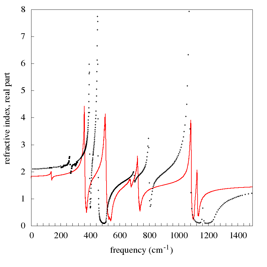
Figure 7: Real part of the refractive index for the ordinary ray as a function of $\omega$, at a temperature of 300 K. Comparison of the calculated curve (red line) with the experimental data, taken from ref. [6] (diamonds) and ref. [10] (squares). Color online.

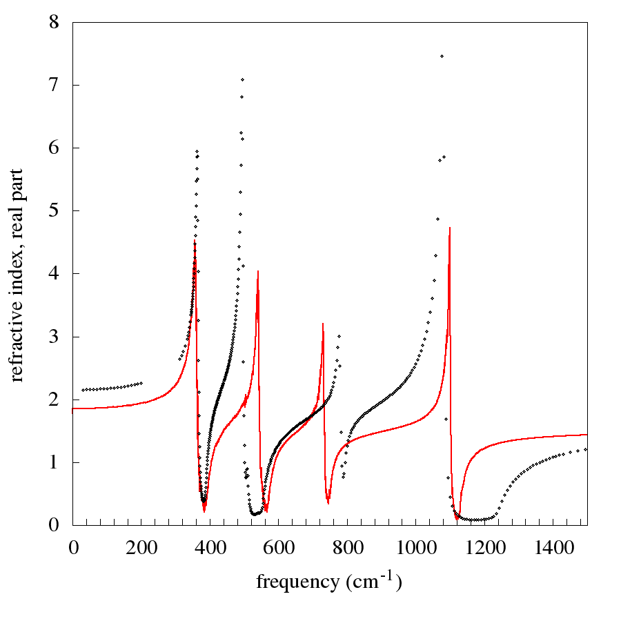
Figure 8: Same as Figure 7 for the extraordinary ray. Here, however, the experimental data (diamonds) are taken only from ref. [6].

We now describe the strategy we followed for optimizing the parameters. The procedure is quite involved, because we have two objectives. On the one hand the system has to admit a global equilibrium configuration, periodic with respect to the primitive cell and furthermore reproducing the $\alpha$ quartz symmetries. On the other hand we require that the normal mode frequencies, calculated at the $\alpha$ equilibrium, reproduce the frequencies observed, both in the infrared spectra and in the Raman ones.

Our procedure was the following one. To start up, we consider the experimental crystallographic configuration of Table 1, given by X ray diffraction, and linearize the equations of motions at that point. So we can determine the normal modes frequencies at the corresponding equilibrium point, as functions of the parameters entering the potential. In this calculation, the symmetries of the crystal are automatically taken into account in the construction of the dynamical matrix, because only some components are directly calculated, all the others being derived by symmetry transformations. As a consequence, the modes are correctly grouped into the three irreducible representations of the symmetry group, namely 4 $A_{1}$ modes, 4 $A_{2}$ modes and 8 degenerate $E$ modes, so that a total of 16 distinct frequencies are obtained. Such properties are reflected in the components of an electric dipole moment vector $\boldsymbol{\mu}$ that we associate to each mode by multiplying the Cartesian displacement of each atom by its effective charge and summing all the vectors thus obtained (see Table 3). This gives an easy criterion for the correct identification of frequencies in the minimization procedure, i.e. in the search for the parameters of the potential that minimize the function

$$W=\frac{1}{16}\sum_{i}^{16}\left(\frac{\omega_{i}-\omega^{ex}_{i}}{\omega^{ex}_{i}}\right)^{2}\ ,$$ (7)

where $\omega^{ex}_{i}$ are the experimental values. This optimization procedure was performed using a simulated annealing algorythm [11], especially useful for multivariate functions. Actually this algorithm provides many different solutions to the optimization problem, possibly due to the presence of many local minima in the function that has to be minimized.

Then, for any single set of parameters obtained we determine the corresponding equilibrium position and the corresponding set of normal mode frequencies. The set of parameters is accepted if the calculated equilibrium position is sufficiently near to the experimental one of $\alpha$ quartz, the frequencies are sufficiently near to the experimental ones, and furthermore the $\alpha$ structure is stable up to sufficiently high temperatures. No set of parameters found gave an agreement for the frequencies better than about 6–7%.

Other attempts were as follows. We started from the power $n=6$ entering (2), letting $n$ be a free parameter, different for each pair, adapting the cutoff parameter to each choice. No substantial improvement was obtained. Then we changed completely the form of the potentials, using Lennard–Jones ones. But this gave a drastic worsening of the results.

These facts show that the results depend in a very sensitive way on the form of the potentials. In order to bypass this problem we decided to restrict our studies to the linear model, assigning as parameters directly the elastic constants. In such a way one even eliminates the constraint that the elastic constants should be defined in terms of first and second derivatives of a given potential. However, no progress was obtained.

As a last resort, we eliminated the neutrality constraint (1) on the effective charge, by assuming both charges to be free parameters, but again without substantial improvement.

Actually, in the whole literature we were unable to find a paper in which the calculated frequencies agree with the experimental ones, in the mean, better than 3%, which is the result obtained in the old paper [12]. In such a paper a linear model is considered, which takes into account also the polarization of oxygen ions as a free parameter. However, the maximum error was larger than 7%.

In the more recent paper [13], a nonlinear model was investigated by MD simulations. Both the short range potentials and the ions polarizability were obtained through ab initio computations, but again, in the very words of the authors, “The calculated frequencies are systematically underestimated, but differences are below 7%–8%.”. The authors point out that their results constitute an improvement with respect to those of previous works, for example those of paper [14], in which “The discrepancy in the lower energy bending vibrations is somewhat higher, usually around 10–20%”. The authors of [13] ascribe the improvement to the fact of having taken the ions’ polarization into account.

Neither does the consideration of three–body potentials, apparently, improve the agreement between computed and observed frequencies. For example, in paper [9] the errors can reach 20% for some modes (see their Table V), as also occurs in paper [15] where for example (see fig. 10) one of the computed lines lies near 600 cm^-1, against the observed value near to 500 cm^-1.

We interpret these facts as indicating that some structural deficiency is present in all models (including ours) that have been considered. Such a deficiency was sometimes acknowledged. For example, in paper [16] it is stated that “The deviations of the calculation with respect to the experiment are not random, but systematic: the higher phonon frequencies, above the mean, are invariably too low with respect to the experiment, while the lower frequencies are invariably too high.”. These facts are usually ascribed to some deficiency in the short range potentials. We conjecture instead that it is the way of dealing with the long–range forces that should play a particularly relevant role in this connection. Indeed, the experimental measures suggest the existence of a splitting between the longitudinal modes and the transverse ones, that should be due to the long–range forces. On the other hand this splitting is actually the feature that the considered models fail to properly describe. We intend to come back to this point in a further work.

Acknowledgments. We thank G. Grosso, G. Pastori Parravicini, N. Manini and G. Onida for useful discussions. The use of computing resources provided by CINECA is also gratefully acknowledged.

sym.	exp.	calc.	$\mu_{x}$	$\mu_{y}$	$\mu_{z}$
	freq.	freq.
	1162	1125	-0.1947	0.1903	0
		1125	-0.1903	-0.1947	0
	1072	1083	0.3479	-0.4105	0
		1083	-0.4105	-0.3479	0
	795	727	0.3032	-0.1175	0
		727	-0.1175	-0.3032	0
	697	675	0.1058	0.1061	0
		675	-0.1061	0.1058	0
$E$	450	506	0.4470	0.2172	0
		506	0.2172	-0.4470	0
	394	359	-0.3075	0.0309	0
		359	-0.0309	-0.3075	0
	265	258	-0.0010	0.0010	0
		258	0.0010	0.0010	0
	128	141	0.0435	0.0072	0
		141	0.0072	-0.0435	0
	1080	1101	0	0	-0.5871
$A_{2}$	778	732	0	0	0.3754
	495	544	0	0	0.4078
	364	358	0	0	-0.4294
	1085	1074	0	0	0
$A_{1}$	464	474	0	0	0
	356	355	0	0	0
	207	232	0	0	0

Table 3: Normal modes of $\alpha$ quartz grouped by symmetry. Experimental frequencies (from [17]) and calculated frequencies in cm^-1 are reported, together with the calculated components of the dipole moment $\boldsymbol{\mu}$ for each mode.

References

- [1] Gangemi F., Carati A., Galgani L., Gangemi R., Maiocchi A., Europhys. Lett 110, (2015) 47003.
- [2] Spitzer W.G., Kleinman D.A., Phys. Rev. 121, (1961) 1324.
- [3] Kihara K., Eur. J. Mineral. 2, (1990) 63.
- [4] Tsuneyuki S., Tsukada M., Aoki H., Matsui Y., Phys. Rev. Lett. 61, (1988) 869.
- [5] Kramer G. J., Farragher N. P., van Beest B. W. H., van Santen R. A., Phys. Rev. B 43, (1991) 5068.
- [6] Palik E., Handbook of optical constants of solids (Academic Press, Amsterdam) (1998) , p. 719.
- [7] Carati A., Galgani L., Eur. Phys. J. D 68, (2014) 307.
- [8] Tsuneyuki F., Aoki H., Tsukada M., Matsui Y., Phys. Rev. Lett 64, (1990) 776.
- [9] Ma W., Garofalini S.H., Phys. Rev. B 73, (2006) 174109.
- [10] Cummings K. D., Tanner D. B., J. Opt. Soc. Am. 70, (1980) 123.
- [11] Kirkpatrick S., Gelatt Jr. C. D., Vecchi M. P., Science 220, (1983) 671
- [12] Iishi K., Zeits. f. Kristall. 144, (1976) 289.
- [13] Liang Y., Miranda C.R., Scandolo S., J. Chem. Phys 125, (2006) 194524.
- [14] Tse S., Klug D.D., J. Chem. Phys. 95, (1991) 9176.
- [15] Huang L., Kieffer J., J. Chem Phys. 118, (2003) 1487.
- [16] Della Valle R.G., Andersen H.G., J. Chem. Phys. 94, (1991) 5056.
- [17] Scott J.F., Porto S.P.S., Phys. Rev. 161, (1967) 903.