Large X-ray Flares on Stars Detected with MAXI/GSC: A Universal Correlation between the Duration of a Flare and its X-ray Luminosity

Abstract

23 giant flares from 13 active stars (eight RS CVn systems, one Algol system, three dMe stars and one YSO) were detected during the first two years of our all-sky X-ray monitoring with the gas propotional counters (GSC) of the Monitor of All-sky X-ray Image (MAXI). The observed parameters of all of these MAXI/GSC flares are found to be at the upper ends for stellar flares with the luminosity of $10^{31-34}$ ergs s^-1 in the 2–20 keV band, the emission measure of 10^54-57 cm^-3, the $e$-folding time of 1 hour to 1.5 days, and the total radiative energy released during the flare of 10^34-39 ergs. Notably, the peak X-ray luminosity of 5${}^{+4}_{-2}\times 10^{33}$ ergs s^-1 in the 2–20 keV band was detected in one of the flares on II Peg, which is one of the, or potentially the, largest ever observed in stellar flares. X-ray flares were detected from GT Mus, V841 Cen, SZ Psc, and TWA-7 for the first time in this survey. Whereas most of our detected sources are multiple-star systems, two of them are single stars (YZ CMi and TWA-7). Among the stellar sources within 100 pc distance, the MAXI/GSC sources have larger rotation velocities than the other sources. This suggests that the rapid rotation velocity may play a key role in generating large flares. Combining the X-ray flare data of nearby stars and the sun, taken from literature and ou r own data, we discovered a universal correlation of $\tau\propto L_{\rm X}^{0.2}$ for the flare duration $\tau$ and the intrinsic X-ray luminosity $L_{\rm X}$ in the 0.1–100 keV band, which holds for 5 and 12 orders of magnitude in $\tau$ and $L_{\rm X}$, respectively. The MAXI/GSC sample is located at the highest ends on the correlation.

1 Introduction

Cool stars, which have spectral types of F, G, K, and M, are known to show X-ray flares. The flares are characterized with the fast-rise and slow-decay light curve. The flares generally accompany the rise and decay in the plasma temperature. The general understanding, based on the numerous studies of solar flares, is that such features arise as a consequence of a sudden energy release and relaxation process in the reconnection of magnetic fields on/around stellar surfaces. In solar flares, the reconnection, which occurred in somewhere at large coronal heights, accelerates primarily electrons (and possibly ions) up to MeV energies, and the electrons precipitate along the magnetic fields into the chromosphere, suddenly heating the plasma at the bottom of the magnetic loop to very high temperatures. A large amount of plasma streams from the bottom to the top of the magnetic loop, while cooling has already started by that time. The flare temperature thus peaks before the Emission Measure (EM) does, or analogously, harder emission peaks before softer emission.

Numerous studies on flare stars have been made with pointing observations. For the reviews, see Pettersen (1989), Haisch et al. (1991), Favata & Micela (2003), Güdel (2004), and references therein. However, we cannot yet answer some fundamental questions, such as how large a flare a star can have, and how very large flares are generated. The poor understanding is rooted in the fact that the larger flares occur less frequently. Hence, all-sky monitoring is crucial to detect such large flares.

X-ray all-sky monitors like Ariel-V/SSI, GRANAT/WATCH, and Swift/BAT have detected some large stellar flares. Using the data of Ariel-V/SSI spanning for 5.5 years, Pye & McHardy (1983) and Rao & Vahia (1987) detected in total twenty flares from seventeen stellar sources, including ten RS CVn systems and seven dMe stars. Rao & Vahia (1987) showed that there is a positive correlation between the bolometric luminosity and the X-ray peak luminosity. GRANAT/WATCH detected two X-ray transients, which have a counterpart of a flare star in their respective positional error boxes (Castro-Tirado et al., 1999). Swift with BAT prompted the follow-up observations with XRT after detecting large flares from an RS CVn system II Peg (Osten et al., 2007) and that from a dMe star EV Lac (Osten et al., 2010). Flares from two other RS CVn stars (CF Tuc and UX Ari) have been detected with Swift/BAT (Krimm et al., 2013).

Following successful detections of large flares with all-sky X-ray surveys, we executed a survey of stellar flares with the Monitor of All-sky X-ray Image (MAXI; Matsuoka et al. (2009)). MAXI is a mission of an all-sky X-ray monitor operated in the Japanese Experiment Module (JEM; Kibo) on the International Space Station (ISS) since 2009 August. It observes an area in the sky once per 92 min orbital cycle, and enables us to search for stellar flares effectively. In this paper, we report the results with the gas proportional counters (GSC) of MAXI obtained by the first two-years operation from 2009 August to 2011 August. The results with the CCD camera of MAXI (SSC) will be given elsewhere. We describe the MAXI observation in $\S$2, our flare-search method and the results in $\S$3, then discuss the properties of the detected flares and the flare sources in $\S$4.

2 Observations

The MAXI has two types of slit cameras, the GSC and SSC, both of which incorporate X-ray detectors consisting of gas proportional counters and X-ray CCDs, respectively. These detectors cover an energy range of 2 to 30 keV and 0.5 to 12 keV, respectively (Matsuoka et al., 2009; Tsunemi et al., 2010; Tomida et al., 2011; Mihara et al., 2011). As stated in section $\S$1, the observations of stellar flares examined here were conducted by the GSC, which has a larger field of view (FoV) and then sky coverage than SSC. The GSC achieves better sensitivity in the 2–10 keV band than any other X-ray all-sky monitors so far using large-area proportional counters with a low background, and then is preferable to detect stellar flares. The data from 2009 August 15th to 2011 August 15th are used here.

The GSC consists of twelve pieces of proportional counters, which employ resistive carbon-wire anodes to acquire one-dimensional position sensitivity. Each set of two counters forms a single camera unit, of which the GSC has six in total. The overall FoV is a slit shape of $\timeform{160D}\times\timeform{3D}$ in the horizon and zenith directions, respectively, which allows the MAXI to scan the entire sky twice as the ISS moves; i.e., MAXI/GSC can scan 97% of the entire sky with each ISS orbit. When the ISS passes high background regions such as the South Atlantic Anomaly, the high voltage of the GSC is switched off to protect the proportional counters from damage. Then, the actual sky coverage is about 85% of the whole sky per 92-minute orbital period, 95% per day, and 100% per week.

The point spread function (PSF) in the Anode-Wire Direction is determined by the angular response of the slit-and-slat collimator and the positional response of the position-sensitive gas counter along the anode wire. The collimator is designed to have an angular resolution of 1D.0–1D.5 in FWHM, depending on the X-ray incident angle in the Anode-Wire Direction and X-ray energy. The PSF in the scan direction is determined with the modulated time variations of the detector area, which changes according to the triangular transmission function of the collimator during each transit. The GSC typically scans a point source on the sky during a transit of 40–150 seconds with a FoV of 1D.5-width (FWHM) every 92-minute orbital period. The transit time depends on the source incident angle in the Anode-Wire Direction. The detector area for the target changes according to the triangular transmission function of the collimator during each transit. The peak value is 4–5 cm² per one camera. The detailed performance of the GSC was described by Sugizaki et al. (2011). All the data we used were delivered from the MAXI database system (Negoro et al., 2016).

3 Analysis and Results

3.1 Search for Flaring Stars

In order to search for flares from stars, we used the alert system “nova search” (Negoro et al., 2010). The alert system on the ground swiftly reports X-ray transient events to astronomers worldwide, prompting potential follow-up observations. For a further search, we have created movies of GSC image for each sky area segmented into circles of 10D radii, setting the observation time of one day for one shot. The entire sky is covered with about 200 segments.

From the confirmed transient events, we selected events whose peaks are located within 2D from nearby known stellar sources. The source lists are composed of the catalogs of Torres et al. (2006), López-Santiago et al. (2006), and Riedel et al. (2014). The locations of the X-ray peaks are determined automatically for the sources confirmed by “nova search”, or by eye from the movies for the others. For these selected stellar-flare candidates, we proceeded to the following identification process.

3.2 Significance in Source Detection

We estimated the significance of a detected source with the same method employed in Uzawa et al. (2011), as follows: (1) extracting events within a circle with 1D.5 radius centered at the transient event (“source region”) in the 2–10 keV band, (2) $\sim$10 circle regions, whose radii are all 1D.5, are chosen around the source region (“background circles”), (3) counting the numbers of events in the 2–10 keV band in each background circle, (4) the average of the counts in a background circle is defined as the background level, (5) the standard deviation of the counts in a background circle is regarded as the 1-$\sigma$ background fluctuation, (6) subtracting the background level from the counts in the source region, and the residual is regarded as the source counts, (7) the source counts divided by the 1-$\sigma$ background fluctuation is defined as the source significance.

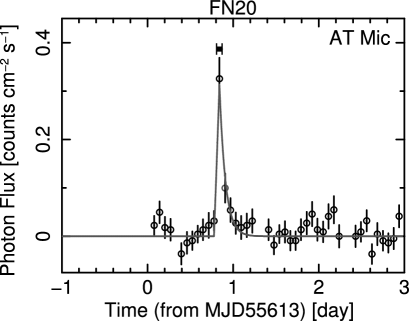
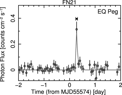
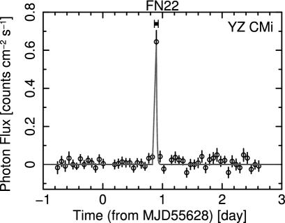
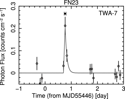
Figure 1: The light curves of twenty-three flares. The data are extracted in the 2–10 keV band. Each data-set shown by an open circle is made from one orbit data, while the datasets in the panels for FN1, 2, 9 and 14 are binned with the data of multiple orbits. The horizontal bar(s) above the major line peak(s) in each panel is the time interval, from which the data are extracted to derive the detection significances and to make the spectral analysis. The light curve of TWA-7 is from Uzawa et al. (2011).

In the first flare on II Peg (FN15 in table $*$ ‣ 1) on 2009 August 20th, the source was in a high-noise area, located close to the wire edge. Thus, we set the background circles in the high-noise area in order to estimate the appropriate level of the background. The time-spans, for which we extracted the data, are indicated in the light curves with horizontal bars in figure 1.

3.3 Reconfirmation of the Source Positions

The number of the stellar flare candidates with the significance larger than 5-$\sigma$ level were twenty-three in total. For these flares, we further performed two-dimensional image fittings to obtain the precise error regions for the X-ray positions. The fitting algorithm is given in Morii et al. (2010). The shape of the region can be approximated with an ellipse with the typical semi-major and semi-minor axes of 0D.7 and 0D.5, respectively, at 90% confidence level. We found that all the error regions still encompass the position of each stellar counterpart in our list, which we had seen within 2D from the X-ray peak. We also confirmed that all the stellar counterparts are listed in the ROSAT bright source catalog (Voges et al., 1999). No other ROSAT bright-sources are in the same error regions for all the events but one; the error region of FN20 (see table $*$ ‣ 1) encompasses AT Mic (1RXS J204151.2$-$322604) and 1RXS J204257.5$-$320320. 1RXS J204257.5$-$320320 is not in our list of nearby sources, and the detailed nature is not known. Moreover, certainly no X-ray variation has ever been reported. Then we regard that the transient occurred on the established flare star, AT Mic. The dates of each flare, the error regions, the X-ray counts rates, the significant levels, and the stellar counterparts are summarized in table $*$ ‣ 1.

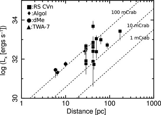
Figure 2: log-log plot of X-ray luminosity in the 2–20 keV band of flares vs. distance from active stars detected with MAXI/GSC. The filled squares, filled diamond, filled circles and filled triangle show RS-CVn type stars, Algol, dMe stars and TWA-7, respectively. The detection limit appeared to be roughly 10 mCrab in the 2–20 keV band.

The detected twenty-three flares were found to come from thirteen stars; eight RS CVn systems (VY Ari, UX Ari, HR1099, GT Mus, V841 Cen, AR Lac, SZ Psc and II Peg), one Algol-type star (Algol), three dMe stars (AT Mic, EQ Peg and YZ CMi), and one YSO (TWA-7). Note that the detection of the flare from TWA-7 has been already reported in Uzawa et al. (2011). We list the fundamental parameters of the stellar counterparts in table $*$ ‣ 2. Four out of thirteen sources showed flares multiple times. We adopt the source distances listed in table $*$ ‣ 2 when we estimate or discuss the physical parameters in this paper. The distances are all within 100 pc, except that of GT Mus (172 pc). Figure 2 displays the relation between the source distance and $L_{\rm X}$. This implies that our detection limit is roughly 10 mCrab in the 2–20 keV band.

3.4 Timing Analysis

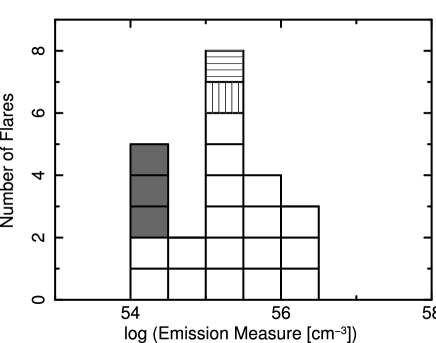
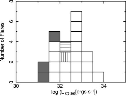
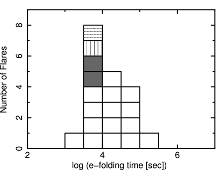
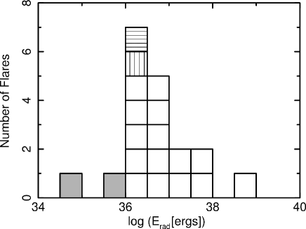
Figure 3: Distribution of the emission measure (top left), X-ray luminosity in the 2–20 keV band (top right), $e$-folding time (bottom left), and total energy (bottom right). The open squares, filled squares, vertical-striped square, and horizontal-striped square show RS-CVn type stars, dMe stars, Algol and TWA-7, respectively.

Figure 1 shows the GSC light-curves of all the detected flares in the 2–10 keV band. In making the light-curves, the data for the sources were extracted from the circles with the radii ranging from 1D.3 to 1D.7, which are selected depending on the signal-to-noise ratio. The backgrounds are extracted from the annuli with the inner and outer radii of 2D and 4D, respectively, except for the following two cases, in which an edge of a wire is close to the source region. In the case of the flare on HR1099 (FN5) on 2010 January 23th, we chose the background region as an annulus with the inner and outer radii of 2D and 3D.5, respectively, to eliminate a high-noise area. As for the first flare on II Peg (FN15) on 2009 August 20th, since the source was more closely located to a wire edge than the HR1099 case, the source region was just in the high-noise area. Thus, in order to remove the appropriate level of the background, we chose the background region as a rectangle of $\timeform{3D.4}\times\timeform{19D}$, removing a central circle with 1D.7 radius. After subtracting the background, all the extracted source-counts were normalized by dividing by the total exposure (in units of cm² s), which is obtained with a time integral of the collimator effective area. We fitted them with a burst model, which is described as a linear rise followed by an exponential decay. The $e$-folding times are shown in table LABEL:para and figure 3, which range from about 1 hour (AR Lac) to 1.5 days (GT Mus).

3.5 Spectral Analysis

We also analyzed X-ray spectra in flare phases. The GSC spectra were extracted during the time interval indicated with the horizontal bars on the light-curves (figure 1), as those used in the estimation of the significance of source detection. We used the same source and the background regions as those used in the timing analysis. Since the photon-statistics are limited, we fitted the spectra with a simple model; a thin-thermal plasma model (mekal: Mewe et al. (1985, 1986); Kaastra (1992); Liedahl et al. (1995)) with the fixed abundance ratios of heavy elements to the solar values. We ignored the interstellar absorption, since all the sources are located within 200 pc and are not in famous molecular clouds. An example of a spectrum with the best-fit model is found in the figure 2 in Uzawa et al. (2011). Table LABEL:para and figure 3 give the best-fit parameters and the distribution of the derived properties (EM, ${\it L_{\rm X}}$, $e$-folding time, the total energy), respectively.

4 Discussion

4.1 Detected Flares and the Source Categories

We detected twenty-three flares, whose X-ray luminosities are $10^{31-34}$ ergs s^-1 in the 2–20 keV band and the emission measures are 10^54-57 cm^-3. The flares released the energy of 10^34-39 ergs radiatively with the $e$-folding times of 1 hour to 1.5 days (see figure 3). All the detected flares are from active stars; eight RS CVn systems, one Algol system, three dMe stars and one YSO, totaling thirteen stars. This confirms that RS CVn systems and dMe stars are intense flare sources, as reported in Pye & McHardy (1983) and Rao & Vahia (1987). The X-ray flares from GT Mus, V841 Cen, SZ Psc, and TWA-7 were detected for the first time in this survey. Notably, II Peg showed the $L_{\rm X}$ of 5${}^{+4}_{-2}\times~{}10^{33}$ ergs s^-1 in the 2–20 keV band at the peak of the flare, which is one of the largest ever observed in the stellar flares.

Most of the flare sources that we detected with MAXI/GSC are multiple-star system (see table $*$ ‣ 2). However, two of them were single stars: TWA-7 (Uzawa et al., 2011) and YZ CMi. In addition, another two (AT Mic and EQ Peg) have, though a binary system, a very wide binary-separation of roughly 6000 , and so are the same as single stars practically. All of these four stars are known to have no accretion disk. These results reinforce the scenario that neither binarity (e.g. Getman et al. (2011)) nor accretion (e.g. Kastner et al. (2002), Argiroffi et al. (2011)), nor star-disk interaction (e.g. Hayashi et al. (1996), Shu et al. (1997), Montmerle et al. (2000)) is essential to generate large flares, as has been already discussed in Uzawa et al. (2011).

According to the catalog of active binary stars (Eker et al., 2008), 256 active binaries (e.g. RS CVn binaries, dMe binaries etc.) are known within the distance of 100 pc from the solar system. However, we detected flares from only ten of them. Four of them (UX Ari, HR1099, AR Lac and II Peg) exhibited flares more than twice.

4.2 X-ray Activity on Solar-type Stars

As for the solar-type stars, fifteen G-type main-sequence stars are known within the 10-pc distance (from AFGK “bright” stars within 10 parsecs). The MAXI/GSC has not detected any X-ray flares from these stars. The nearest G-type star is $\alpha$ Cen A (G2 V) at the distance of 1.3 pc (Söderhjelm, 1999). The upper limit on the $L_{\rm X}$ of $\alpha$ Cen A is estimated to be 2$~{}\times~{}10^{28}$ ergs s^-1, based on the detection limit of 10 mCrab with MAXI/GSC. This is consistent with the X-ray luminosities observed in solar flares; $L_{\rm X}$ is mostly lower than $10^{27}$–$10^{28}$ ergs s^-1 (Feldman et al., 1995). However, large X-ray flares with the respective $L_{\rm X}$ of $10^{29}$ ergs s^-1 and $2~{}\times~{}10^{31}$ ergs s^-1 have been observed from ordinary solar-type stars $\pi^{1}$ UMa (Landini et al., 1986) and BD$+$10^∘2783 (Schaefer et al., 2000). Schaefer et al. (2000) called such flares “superflares”. So far, very few extensive studies have been made in the X-ray band and reported to give any good constraints on the frequency of the occurrence of “superflares” in the band. Our MAXI/GSC two-year survey is the best X-ray study of this kind. From our result, we can claim that the flares with $L_{\rm X}$ of larger than $1~{}\times~{}10^{30}$ ergs s^-1 must be very rare for solar-type stars.

4.3 $EM$ vs. $kT$ and the Derived Loop Parameters

Figure 4 shows a plot of $EM$ vs. plasma temperature $(kT)$ for the flares in our study of the MAXI/GSC sources, together with solar flares (Feldman et al., 1995), solar microflares (Shimizu, 1995), and flares from the stars in literature (see table 4 for the complete set of references). All of the plotted samples are roughly on the universal correlation over orders of magnitude (Feldman et al. (1995), Shibata & Yokoyama (1999)). Our sample is located at the high ends in the correlation for both the temperatures and emission measures.

Now, we consider the two important physical parameters of flares, that is, the size and magnetic field. Shibata & Yokoyama (1999) formulated the theoretical $EM$-$kT$ relations for a given set of a loop-length and magnetic field as equations (5) and (6) in their paper (see figure 4 for a few representative cases). We calculated the loop-length and magnetic-field strength for each of the observed flares with MAXI-GSC, based on the relations (Shibata & Yokoyama, 1999), as listed in table LABEL:para. The magnetic field of our sample is comparable with those of flares on the Sun ($\sim$15–150 G). On the other hand, our sample has orders of magnitude larger sizes of flare loops than those on the Sun ($<$0.1 ). Especially noteworthy ones among our sample are the two largest flares relative to their binary separations, FN4 from UX Ari and FN16 from II Peg. Their loop lengths are 10 and 20 times larger than their respective binary separations, which are unprecedentedly large among stellar flares.

The extraordinary large loop lengths could possibly be an artifact due to the systematic error in the model by Shibata & Yokoyama (1999). In fact, their derived loop lengths are 10 times larger than those obtained by Favata et al. (2001), who used a hydrodynamic model by Reale & Micela (1998). In Shibata & Yokoyama (2002), which is the follow-up paper of Shibata & Yokoyama (1999), it is argued that their derived loop length could be reduced to roughly 1/10 if the two assumptions (the points 3 and 4 mentioned in the footnote below) are altered. In our MAXI sample, even if the true loop sizes are 1/10 of the above-estimated values as a conservative case, the largest ones are 0.2–5 times larger than their binary separation and so are still large.

4.4 Duration vs. X-ray Luminosity

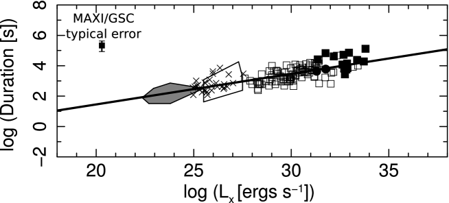
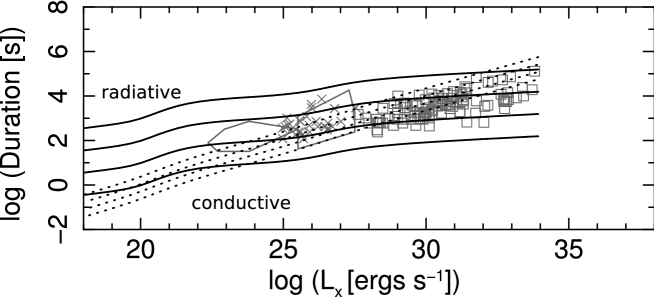
Figure 5: Top panel: Log-log plot of the duration of flares vs. X-ray luminosity in the 0.1–100 keV band. Our best-fit model is inserted with a broad solid line. The filled and open symbols are the same as those in figure 2 and 4, respectively. We superpose three sets of data of solar flares: X marks, large open pentagon and large gray region, taken from Pallavicini et al. (1977), Veronig et al. (2002) and Shimizu (1995), respectively. The typical error for MAXI/GSC sources is also inserted. Middle panel: The theoretical relations of the radiative cooling model (solid line) and conductive cooling model (dotted line) are overlaid for the non-dimensional parameter $\alpha$ of 0.3, 1 and 3 from the top to bottom lines, respectively, for both the models, where $n_{\rm e}$ is fixed to $10^{11}~{}{\rm cm}^{-3}$. Bottom panel: The same as the middle panel, but with $\alpha$ fixed to 1 and $n_{\rm e}$ varied instead for $n_{\rm e}~{}=$ $10^{10}$, $10^{11}$, $10^{12}$ and $10^{13}~{}{\rm cm}^{-3}$, corresponding to the 4 lines from top to bottom, respectively, for each model.

We search for potential correlations in various plots to study what are the deciding factors to generate large stellar flares and to which extent. Figure 5 plots the duration of flares ($\tau_{\rm lc}$) vs. the intrinsic X-ray luminosity ($L_{\rm X\_bol}$) in the 0.1–100 keV band for the stars detected with MAXI/GSC and with other missions (see table 4 for the complete set of references). Here, we have introduced $L_{\rm X\_bol}$ in order to take all the radiative energy into our calculation . Solar flares (Pallavicini et al. (1977), Shimizu (1995), Veronig et al. (2002)) too are superposed . The data points of the MAXI/GSC flares are found to be located at the highest ends in both the $L_{\rm X\_bol}$ and duration axes among all the stellar flares. The plot indicates that there is a universal correlation between $L_{\rm X\_bol}$ of a flare and its duration, such that a longer duration means a higher $L_{\rm X\_bol}$. Remarkably, the correlation holds for wide ranges of parameter values for $10^{22}$$\lesssim L_{\rm X\_bol}\lesssim 10^{34}$ ergs s^-1 and $10^{1}$ $\lesssim\tau_{\rm lc}\lesssim 10^{6}$ s. Using the datasets of the stellar flares detected with MAXI (this work) and other missions (table 4), and the solar flares reported by Pallavicini et al. (1977), we fitted the data with a linear function in the log-log plot and obtained the best-fit function of

$$\tau_{\rm lc}=(1.1^{+4.7}_{-0.9})\times 10^{4}~{}\left(\frac{L_{\rm X\_bol}}{10^{33}~{}{\rm ergs~{}s^{-1}}}\right)^{0.20\pm 0.03}{\rm sec},$$ (1)

where the errors of both the coefficient and the power are in 1-$\sigma$ confidence level. The best-fit model is shown with a solid line in figure 5 top panel. We found that the best-fit model agrees also with the range of the data for solar microflares reported by Shimizu (1995), even though the luminosities $L_{\rm X\_bol}$ of their data are smaller than $\sim 10^{25}$ ergs s^-1, whereas those used for our fitting are larger than that.

For comparison, Veronig et al. (2002) and Christe et al. (2008) have derived similar power-law slope as ours, $\sim$0.33 for the GOES data and $\sim$0.2 for the RESSI data, respectively, though with the limited energy bands. The ranges of their luminosities are $L_{\rm X}=10^{23.5-25.5}$ ergs s^-1 in the 3.1–24.8 keV band and $L_{\rm X}=10^{22.5-25.5}$ ergs s^-1 in the 6–12 keV band, respectively.

In the following subsections, we discuss the plausible models to explain this positive correlation, examining three potentially viable scenarios: the radiative-cooling dominant, conductive-cooling dominant, and propagating-flare models. Note that we have chosen the former two models for simplicity and examine them separately, although it is expected, as most star-flare models assume, that both radiation and conduction are present in a flare and that the latter is active early in the decay and the former is, later (e.g. Shibata & Yokoyama (2002), Cargill (2004), Reale (2007)). We assume that the duration of a flare $\tau_{\rm lc}$ represents the cooling time of the heated plasma when we examine the radiative- and conductive-cooling dominant models.

4.4.1 Radiative Cooling Model

First, we consider the condition where the radiative cooling is dominant. Since the thermal energy is lost via radiation, $\tau_{\rm lc}$ and the radiative cooling time $\tau_{\rm rad}$ are given by,

$$\tau_{\rm lc}\simeq\tau_{\rm rad} = \frac{3n_{\rm e}kT}{n_{\rm e}^{2}~{}F(T)}=\frac{3kT}{n_{\rm e}~{}F(T)},$$ (2)

where $n_{\rm e}$ and $F(T)$ are the electron density and radiative loss rate, respectively. We obtained the radiative loss rate, using the CHIANTI atomic database (version 8.0) and the ChiantiPy package (version 0.6.4) .

On the other hand, based on the plot of $EM$ vs. $kT$ (figure 4), we confirm that most of the observed data of stellar and solar flares are confined in the region of 15 G $<B<$ 150 G, where $B$ is magnetic field strength. The region is mathematically described as

$$EM\simeq 10^{48}~{}\alpha^{-5}\left(\frac{T}{10^{7}~{}{\rm K}}\right)^{17/2}~{}{\rm cm^{-3}}~{},$$ (3)

where $\alpha$ is a non-dimensional parameter ranging between 0.3 and 3. Since the derived $EM$ and $F(T)$ compose $L_{\rm X\_bol}$ as

$$L_{\rm X\_bol}=EM~{}F(T)~{},$$ (4)

we obtain, combining it with equation (3),

$$L_{\rm X\_bol}\simeq 10^{48}~{}\alpha^{-5}\left(\frac{T}{10^{7}~{}{\rm K}}\right)^{17/2}~{}F(T)~{}.$$ (5)

Now that both $\tau_{\rm lc}$ and $L_{\rm X\_bol}$ have been parameterized with the temperature $T$, we insert solid lines in figure 5 as their relation for radiative-cooling dominant model.

Observationally, the electron density $n_{\rm e}$ was measured to be $10^{11}~{}{\rm cm^{-3}}$ in flares of Proxima Centauri with a high-resolution spectroscopy in the X-ray band (Güdel et al., 2002). In the solar flares, $n_{\rm e}$ of $10^{10-11}~{}{\rm cm^{-3}}$ has been calculated from the $EM$ and the volume of the loop (Pallavicini et al., 1977). Some other spectroscopic observations of solar flares have indicated a wide range of $n_{\rm e}$; $10^{11-13}~{}{\rm cm^{-3}}$ (see references in Güdel (2004)). Therefore, we derived the permitted ranges for radiative cooling plasma in the following two cases: (1) $n_{\rm e}~{}=~{}10^{11}~{}{\rm cm^{-3}}$ and $\alpha$= 0.3–3 (figure 5 middle panel), (2) $n_{\rm e}~{}=~{}10^{10-13}~{}{\rm cm^{-3}}$ and $\alpha$ = 1 (figure 5 bottom panel). With the wide permitted range, the figures indicate that radiative cooling explains all the flares in our dataset.

4.4.2 Conductive Cooling Model

Second, we consider the condition where the conductive cooling is dominant, assuming a semicircular loop of the flare with the cross-section of $\pi\left(\frac{l}{10}\right)^{2}$ for the half-length $l$, which is often observed in solar flares. In this case, $\tau_{\rm lc}$ and the conductive cooling time $\tau_{\rm con}$ are given by

$$\tau_{\rm lc}\simeq\tau_{\rm con} = \frac{3n_{\rm e}kT}{10^{-6}~{}T^{7/2}~{}l^{-2}}$$ (6)

$$= 1.3\times 10^{2}~{}\left(\frac{n_{\rm e}}{10^{11}~{}{\rm cm^{-3}}}\right)$$

$$\times \left(\frac{T}{10^{7}~{}{\rm K}}\right)^{-5/2}\left(\frac{l}{10^{9}~{}{\rm cm}}\right)^{2}{\rm sec}.$$

On the other hand, a fraction of the thermal energy is observed as radiation. The luminosity $L_{\rm X\_bol}$ and $EM$ for the temperature $T$ are written as equations (4) and (3), respectively. With the plasma volume of $\frac{\pi}{50}l^{3}$, $EM$ is also written as,

$$EM=\frac{\pi}{50}~{}n_{\rm e}^{2}~{}l^{3}~{}.$$ (7)

Combining equations (3), (6) and (7) gives

$$\tau_{\rm lc}\simeq 1.3\times 10^{5}\left(\frac{50}{\pi}\right)^{2/3}~{}\alpha^{-10/3}~{}n_{\rm e}^{-1/3}~{}\left(\frac{T}{10^{7}~{}{\rm K}}\right)^{19/6}~{}.$$ (8)

Now that both $\tau_{\rm lc}$ and $L_{\rm X\_bol}$ have been parameterized with the temperature $T$, we insert dotted lines in figure 5 as their relation for conductive-cooling dominant model. The values of $n_{\rm e}$ and $\alpha$ are varied independently within the ranges of $10^{10}$ $\lesssim n_{\rm e}\lesssim$ $10^{13}~{}{\rm cm^{-3}}$ and 0.3 $\lesssim\alpha\lesssim$ 3, respectively. The figure indicates that the model and the data overlap with each other in the given parameter space.

4.4.3 Propagating Flare Model

Third, we examine spatially propagating flare, like two-ribbon flares seen on the Sun. The total energy released during a flare via radiation, $E_{\rm rad}$, is described as

$$E_{\rm rad}\simeq\tau_{\rm lc}L_{\rm X\_bol}~{}.$$ (9)

On the other hand, $E_{\rm rad}$ originates from thermal energy confined in the plasma, and the thermal energy comes from stored magnetic energy, $E_{\rm mag}$. Then, it can be also written as

$$E_{\rm rad}=f~{}E_{\rm mag}=\frac{f~{}B^{2}~{}D^{3}}{8\pi}~{},$$ (10)

where $f$ is the energy conversion efficiency from magnetic energy to that released as radiation, and $D$ is the scale length of the flaring region. When we assume that the magnetic reconnection propagates with the speed $v$, $\tau_{\rm lc}$ satisfies the following formula

$$\tau_{\rm lc}=D/v~{}.$$ (11)

Eliminating $E_{\rm rad}$ and $D$ with the equations (9), (10) and (11), we obtain

$$\tau_{\rm lc} \simeq 1.2\times 10^{4}\left(\frac{f}{0.1}\right)^{1/2}\left(\frac{B}{50~{}{\rm G}}\right)^{-1}$$ (12)

$$\times \left(\frac{v}{3\times 10^{7}~{}{\rm cm~{}s^{-1}}}\right)^{-3/2}\left(\frac{L_{\rm X\_bol}}{10^{33}~{}{\rm ergs~{}s^{-1}}}\right)^{1/2}{\rm sec}.$$

If the values of $f$, $B$ and $v$ are common among stars,

$$\tau_{\rm lc}\propto L_{\rm X\_bol}^{1/2}~{}.$$ (13)

The power of $L_{\rm X\_bol}$ is slightly larger than what we obtained.

4.5 Origin of Large Flares

4.5.1 Rotation Velocity

The positive correlation between quiescent X-ray luminosity and rotation velocity has been reported by Pallavicini (1989) and in subsequent studies. However, no studies have been published about this type of correlation for the flare luminosity. Compiling our data sample and those in literature, we search for the potential correlation of this kind.
We plot the total energy released during a flare (i.e., $E_{\rm rad}$) vs. the square of rotation velocity ($v_{\rm rot}^{2}$) in figure 6, where $E_{\rm rad}$ is derived by multiplying $L_{\rm X}$ in the 2–20 keV band by the $e$-folding time of the flare decaying phase. From figure 6, we find that the MAXI sample is concentrated at the region of the high rotation velocity and the large total energy. This is the first indication with an unbiased survey that stellar sources with higher rotation velocities can have a very high $E_{\rm rad}$.

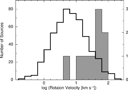
Figure 7: Histogram of rotation velocities. The gray bars indicate the MAXI/GSC-detected sources within 100 pc with the scale displayed on the right-hand Y-axis. The white bars indicate active binaries and X-ray-detected stellar sources both within 100 pc (from Eker et al. (2008) and Wright et al. (2011)), with the scale displayed on the left-hand Y-axis, from which the MAXI/GSC-detected sources are excluded.

In order to validate this tendency further, we made two histograms of the number of sources as a function of the star-rotation velocity for flare sources. One is for our MAXI/GSC sample, and the other is for cataloged nearby stars from the literature (active binaries; Eker et al. (2008), X-ray-detected stellar sources; Wright et al. (2011)). Both the samples are within 100 pc distance, and from the latter sample, MAXI/GSC sources are excluded. Figure 7 shows the two histograms. The MAXI/GSC sources have the median logarithmic rotation velocity of 1.52 in units of log (km s^-1) with the standard deviation of 0.37 dex. On the other hand, the undetected sources with MAXI/GSC have the median logarithmic value of 0.80 in the same units with the standard deviation of 0.52 dex. Therefore, the rotation velocities of the MAXI sources, which have shown huge flares as reported in this paper, are significantly higher than those of the other active stars that are comparatively quiet. This supports that the sources with faster velocities generate larger flares.

4.5.2 Stellar Radius

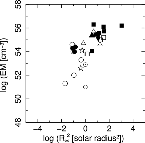
Figure 8: Log-log plot of emission measure vs. the square of radius. The symbols are the same as in figure 6. The upper open circle with a dot indicates $\pi^{1}$ UMa, while the lower does the Sun.

We investigate whether the MAXI sources and/or the size of the flare-emitting region have any common characteristics or correlations in their stellar radii.
Figure 8 plots $EM$ vs. the square of the stellar radius ($R_{*}^{2}$) for the stars detected with MAXI/GSC and those detected with other missions (see table 4 for the complete set of references). Though the sample is limited, a hint of the positive correlation between $EM$ and $R_{*}^{2}$ is seen at least in the MAXI/GSC sources.

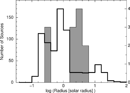
Figure 9: Histogram of stellar radii. The gray bars indicate the MAXI/GSC sources within 100 pc with the scale displayed on the right-hand Y-axis. The white bars indicate active binaries and X-ray-detected stellar sources both within 100 pc (from Eker et al. (2008) and Wright et al. (2011)), with the scale displayed on the left-hand Y-axis, from which the MAXI/GSC-detected sources are excluded.

We also made a number-distribution histogram as a function of the radius in figure 9, similar to figure 7. From figure 9, we find MAXI/GSC sources are concentrated at the radii of about 3 and 0.3 , which correspond to RS CVn-type and dMe stars, respectively. On the other hand, the undetected sources with MAXI/GSC are widely distributed in figure 9, which implies that the magnitude of flares is not as sensitive to the stellar radius as to the rotation velocity.

5 Summary

1. During the two-year MAXI/GSC survey, we detected twenty-three energetic flares from thirteen active stars (eight RS-CVn stars, three dMe stars, one YSO, and one Algol type star). The physical parameters of the flares are very large for stellar flares in all of the followings: the X-ray luminosity $L_{\rm X}$ ($10^{31-34}$ ergs s^-1 in the 2–20 keV band), the emission measure $EM$ (10^54-57 cm^-3), the $e$-folding time (10^3-6 s), and the total energy released during the flare (10^34-39 ergs).

2. The flares from GT Mus, V841 Cen, SZ Psc and TWA-7 were detected for the first time in the X-ray band. From II Peg, we detected one of the largest flares among stellar flares with $L_{\rm X}$ of 5${}^{+4}_{-2}~{}\times~{}10^{33}$ ergs s^-1 in the 2–20 keV band. Whereas most of the sources detected with MAXI/GSC are multiple-star systems, two of them (YZ CMi and TWA-7) are single, which are known to have no accretion disk. These results reinforce the scenario that none of binarity, accretion, and star-disk interaction is essential to generate large flares, as has been already discussed in Uzawa et al. (2011).

3. The survey showed that the number of the sources that show extremely large flares is very limited; only ten out of the 256 active binaries within the 100 pc distance have been detected, while four of the ten sources showed flares multiple times. We detected no X-ray flares from solar-type stars, despite the fact that fifteen G-type main-sequence stars lie within 10-pc distance. This implies that the frequency of the superflares from solar-type stars, which has $L_{\rm X}$ of more than $1~{}\times~{}10^{30}$ ergs s^-1, is very small.

4. On the $EM$–$kT$ plot, our sample is located at the high ends in the universal correlation, which ranges over orders of magnitude (Feldman et al. (1995), Shibata & Yokoyama (1999)). According to the theory of Shibata & Yokoyama (1999), our sample has the similar intensity of magnetic field to those detected on the Sun ($\sim$15–150 G), but has orders of magnitude larger flare-loop sizes than those on the Sun ($<$ 0.1 ). The largest two loop sizes from UX Ari and II Peg are huge, and are much larger than the binary separations.

5. We plotted the duration vs $L_{\rm X\_bol}$, using the data of solar and stellar flares in literature and the data of the flares on MAXI/GSC sources. The plot indicates that there is a universal positive correlation between $L_{\rm X\_bol}$ of a flare and its duration, such that a longer duration means a higher $L_{\rm X\_bol}$. The correlation holds for the wide range of parameter values; 12 and 5 orders of magnitude in $L_{\rm X\_bol}$ and duration, respectively. Our sample is located at the highest ends on the correlation. From the data, we found that the duration is proportional to $L_{\rm X\_bol}^{0.2}$.

6. Our sample has especially fast rotation velocities with an order of 10 km s^-1. This indicates that the rotation velocity is an essential parameter to generate big flares.

We thank M. Sakano, Y. Maeda, F. Reale, and S. Takasao for useful discussion. This research has made use of the MAXI data, provided by the RIKEN, JAXA, and MAXI teams. This research was partially supported by the Ministry of Education, Culture, Sports, Science and Technology (MEXT), Grant-in-Aid No.19047001, 20041008, 20244015, 20540230, 20540237, 21340043, 21740140, 22740120, 23540269, 16K17667, and Global-COE from MEXT “The Next Generation of Physics, Spun from Universality and Emergence” and “Nanoscience and Quantum Physics”. Y.T. acknowledges financial support by a Chuo University Grant for Special Research.

The process to derive $L_{\rm X\_bol}$ for each dataset

In §4.4, we derived the intrinsic X-ray luminosity $L_{\rm X\_bol}$ in the 0.1–100 keV band from the available observed X-ray data in narrower energy bands (Pallavicini et al. (1977), Shimizu (1995), Veronig et al. (2002)). The process to derive it is as follows.

1. In principle, we derive $L_{\rm X\_bol}$ from the parameters $kT$ and $EM$, using the equation 4. As for the X-ray data of Shimizu (1995) and Veronig et al. (2002), it is necessary to estimate the values of $kT$ and $EM$ from the X-ray luminosities in the GOES band (3.1–24.8 keV) (hereafter $L_{\rm X\_GOES}$). To estimate them, first, we derive the ratios (denoted as $P(T)$) of the X-ray luminosity in the GOES band to that in the 0.1–100 keV band (i.e., $L_{\rm X\_bol}$) as a function of $kT$, using the $apec$ model in $XSPEC$. Next, assuming the empirical relation of $EM$ vs.$kT$ for flares, (equation 3), we obtain $EM$ as a function of $kT$, with the parameter $\alpha$ fixed to one (hereafter $EM(T)$). Combining these parameters with equation 4, the GOES band luminosity is written as

   $$L_{\rm X\_GOES}=L_{\rm X\_bol}~{}P(T)=F(T)~{}EM(T)~{}P(T).$$ (14)

   We can derive $T$ for each $L_{\rm X\_GOES}$, and then obtain $L_{\rm X\_bol}$ with this formula.

2. As for the X-ray data of Pallavicini et al. (1990a), we simply accept the X-ray luminosities in the 0.05–2 keV band in their paper as $L_{\rm X\_bol}$, because the luminosities in the band are estimated to be about 95% of $L_{\rm X\_bol}$. Note that we have used the $apec$ model in $XSPEC$, varying the temperatures in the range of log $T$ = 6.5–7.3 (K), to get the ratio of 95%, where the range for the temperatures is assumed by Pallavicini et al. (1990a).

Table 1: Date and other observed parameters of each flare.

Flare	MJD	UT	Error Ellipse				Count Rate	Significance	Counterpart	Category
			Center(J2000)	Semimajor axis	Semiminor axis	Roll angle
		[YYYY MMM DD HH:MM:SS]	[HH:MM:SS, DDD:MM:SS]	[degree]	[degree]	[degree]	[10-2counts s-1]	[$\sigma$]
FN1	55144.347	2009 Nov 09 08:19:15	02:49:55.49, +31:18:32.34	1.0	0.82	90	1.1	7.4	VY Ari	RS CVn
FN2	55080.193	2009 Sep 06 04:37:45	03:26:33.38, +28:31:36.03	0.6	0.57	90	0.72	9.5	UX Ari	RS CVn
FN3	55662.965	2011 Apr 11 23:09:50	03:26:06.13, +28:49:51.75	0.31	0.26	0	12	14	UX Ari	RS CVn
FN4	55678.049	2011 Apr 27 01:10:25	03:26:09.44, +28:47:41.58	0.44	0.36	110	32	16	UX Ari	RS CVn
FN5	55219.221	2010 Jan 23 05:18:10	03:37:02.86, +00:42:24.30	0.5	0.43	170	17	24	HR1099	RS CVn
FN6	55244.054	2010 Feb 17 01:17:51	03:36:28.02, +00:23:58.80	0.43	0.39	90	0.53	7.1	HR1099	RS CVn
FN7	55503.647	2010 Nov 03 15:31:35	03:39:24.90, +00:19:37.43	1.1	0.73	40	4.5	5.1	HR1099	RS CVn
FN8	55625.878	2011 Mar 05 21:03:45	03:36:24.15, +00:31:51.98	0.31	0.21	12	47	29	HR1099	RS CVn
FN9	55510.015	2010 Nov 11 00:21:07	11:40:43.67, -65:01:44.00	0.44	0.35	15	0.27	10	GT Mus	RS CVn
FN10	55769.137	2011 Jul 27 03:16:43	14:34:07.69, -60:33:54.43	0.49	0.32	0	58	8.7	V841 Cen	RS CVn
FN11	55219.255	2010 Jan 23 06:06:55	22:08:29.83, +45:38:19.77	0.64	0.54	75	22	17	AR Lac	RS CVn
FN12	55376.647	2010 Jun 29 15:31:51	22:06:42.49, +45:40:20.19	0.75	0.56	130	19	6.7	AR Lac	RS CVn
FN13	55785.823	2011 Aug 12 19:45:20	22:14:56.90, +46:15:13.01	2.4	0.96	45	0.71	5.2	AR Lac	RS CVn
FN14	55101.059	2009 Sep 28 01:25:30	23:11:50.76, +02:55:10.28	0.53	0.49	15	3.5	5.7	SZ Psc	RS CVn
FN15	55063.937	2009 Aug 20 22:29:55	23:58:33.24, +28:15:57.20	1.1	0.97	45	2.0	19	II Peg	RS CVn
FN16	55291.166	2010 Apr 05 03:58:30	23:54:58.71, +28:51:27.99	0.74	0.64	20	41	13	II Peg	RS CVn
FN17	55433.679	2010 Aug 25 16:17:55	23:55:01.76, +28:36:48.00	1.1	0.7	153	1.2	9.9	II Peg	RS CVn
FN18	55434.315	2010 Aug 26 07:34:00	23:57:52.31, +28:39:34.00	1.2	9.5	0	0.29	9.6	II Peg	RS CVn
FN19	55561.057	2010 Dec 31 01:22:00	03:07:57.26, +40:50:15.00	0.46	0.33	10	20	11	Algol	Algol
FN20	55613.840	2011 Feb 21 20:10:00	20:43:34.04, -32:13:03.96	0.56	0.52	45	69	19	AT Mic	dMe
FN21	55574.278	2011 Jan 13 06:41:00	23:31:33.68, +19:43:53.94	0.35	0.32	40	36	15	EQ Peg	dMe
FN22	55628.897	2011 Mar 08 21:31:00	07:43:46.70, +03:26:26.16	0.32	0.29	160	39	45	YZ CMi	dMe
FN23	55446.767	2010 Sep 07 18:25:00	10:43:41.64, -33:36:30.75	0.57	0.45	150	14	17	TWA 7	YSO

The time when the maximum luminosity was observed.
Observed count rate in the 2–10 keV band.

Table 2: General properties of stars in our sample.

Object name	HD	Spectral type	Rotation velocity	Radius	a sini	inclination of orbit	$e$	Distance	References
			(km s-1)	(R⊙)	(R⊙)	(degree)		(pc)
VY Ari	17433	K3 V + K4 IV§	10.2	1.90	8.2	57	0.085	44	(1)(2)(3)(4)
UX Ari	21242	G5 V + K0 IV§	41.5	5.78	5.9 (h) / 5.3 (c)	59.2	0	50.2	(3)(4)(5)(6)
HR1099	22468	G5 IV + K1 IV§	59.0	3.30	1.9 (h) / 2.4 (c)	38	0	29	(4)(7)(8)(9)(10)
GT Mus	101379	(A0V+A2V) + (G5III+G8III§)	–	33.0	15	10	0.032	172	(4)(11)(12)(13)
V841 Cen	127535	K1 IV§	–	3.8	4.1	–	0	63	(14)(15)(16)
AR Lac	210334	G2 IV + K0 IV§	73.7	2.68	4.6 (h) / 4.5 (c)	89.4	0	42	(3)(4)(17)(18)(19)
SZ Psc	219113	F5 IV + K1 IV§	80.2	6.0	8.7 (h) / 6.4 (c)	69.8	0	88	(3)(4)(20)(21)
II Peg	224085	K2 IV§ + M0-3 V	–	2.21	4.9	60	0	42	(4)(22)(23)(24)(25)
Algol	19356	B8 V + K2 IV§	–	3.4	14	81.4	0	28.5	(26)(27)(28)(29)
AT Mic	196982	M4.5 V + M4.5 V§	24.6	0.38	5980	–	–	10.2	(30)(31)(32)(33)
EQ Peg	–	M3.5 V + M5 V§	88.5	0.35	5590	30	–	6.5	(34)(35)(36)(37)(38)
YZ CMi	–	M4.5 V§	5.3	0.29	–	–	–	5.9	(31)(34)(39)
TWA-7	–	M2 V§	19.2	1.89	–	–	–	27	(40)(41)

The a and i in a sini show the semi-major axes and inclination angle, respectively. The (h) and (c) show the semi-major axes for the orbit of the hot and cool components, respectively.
The stellar component with the symbol $\S$ has the largest radius in the multiple-star system. As for the values for the radius and the rotation velocity in this table, the components with this symbol are used.
V841 Cen is a single-lined RS CVn binary.
(1) Alekseev & Kozlova (2001) (2) Bopp et al. (1989) (3) Glebocki & Stawikowski (1995) (4) ESA (1997) (5) Carlos & Popper (1971) (6) Duemmler & Aarum (2001) (7) Donati et al. (1997) (8) Donati (1999) (9) Fekel (1983) (10) Lanza et al. (2006) (11) Murdoch et al. (1995) (12) Randich et al. (1993) (13) Stawikowski & Glebocki (1994) (14) Özeren et al. (1999) (15) Strassmeier et al. (1994) (16) Collier (1982) (17) Chambliss (1976) (18) Zboril et al. (2005) (19) Sanford (1951) (20) Eaton & Henry (2007) (21) Jakate et al. (1976) (22) Berdyugina et al. (1998) (23) Marino et al. (1999) (24) O’Neal et al. (2001) (25) Vogt (1981) (26) Richards et al. (2003) (27) Sarna (1993) (28) Singh et al. (1995) (29) van den Oord & Mewe (1989) (30) Lim et al. (1987) (31) Mitra-Kraev (2007) (32) Mitra-Kraev et al. (2005) (33) Wilson (1978) (34) Morin et al. (2008) (35) Pallavicini et al. (1990a) (36) Pettersen et al. (1984) (37) Pizzolato et al. (2003) (38) Hopmann (1958) (39) Reiners et al. (2009) (40) Mamajek (2005) (41) Yang et al. (2008)

Table 3: Best-fit parameters in the fitting, and derived flare parameters.

	$kT$	$EM$	Flux∗	$L_{\rm X(2-20)}^{\dagger}$	$\chi^{2}_{\nu}$ (d.o.f)	${\tau}_{d}^{\ddagger}$	$E_{\rm tot}^{\S}$	$l^{\|}$		$B^{\#}$
	(keV)	($10^{54}$	($10^{-10}{\rm ergs}$	($10^{31}$		(ks)	($10^{35}$	(R⊙)	(binary separation)	(G)
		${\rm cm}^{-3}$)	${\rm cm}^{-2}\hskip 3.01389pt{\rm s}^{-1}$)	${\rm ergs\hskip 3.01389pts}^{-1}$)			ergs)
FN1	5	1	2	5	0.42 (4)	26	10	4	0.4	50
	(2–40)	(0.5–2)	(1–3)	(3–7)		(11–50)	(8–20)	(0.1–20)	(0.01–2)	(10–3000)
FN2	4	24	8	20	1.7 (7)	53	100	30	2	20
	(2–30)	(15–36)	(4–10)	(10–30)		(30–81)	(60–200)	(1–100)	(0.1–8)	(8–600)
FN3	${\geq}$5	60	40	100	0.63(6)	–	–	$\leq$50	$\leq$4	$\geq$20
		(40–80)	(30–50)	(90–200)		–	–
FN4	3	100	40	100	0.60 (2)	24	300	100	10	10
	(2–7)	(70–200)	(8–50)	(30–200)		(10–42)	(60–400)	(20–500)	(2–40)	(3–50)
FN5	5	30	30	30	0.42 (5)	6	20	20	3	30
	(3–10)	(20–40)	(10–40)	(10–40)		(4–8)	(5–30)	(5–70)	(0.8–10)	(10–100)
FN6	${\geq}$4	3	6	6	0.5 (7)	67	40	$\leq$10	$\leq$2	$\geq$30
		(2–4)	(5–7)	(5–7)		(45–93)	(30-50)
FN7	${\geq}$4	4	8	8	0.76 (3)	–	–	$\leq$10	$\leq$ 10	$\geq$30
		(3–6)	(6–11)	(6–11)		–	–
FN8	7	30	50	50	0.33 (3)	14	70	20	2	50
	(3–30)	(20–50)	(2–60)	(2–60)		(11–18)	(2–80)	(2–70)	(0.2–10)	(10–500)
FN9	8	160	8	270	1.8 (7)	130	3500	50	0.6	40
	(4–20)	(130–210)	(2–9)	(90–320)		(89–190)	(1200–4200)	(7–600)	(0.1–7)	(5–300)
FN10	${\geq}$4	40	20	100	0.19 (3)	7	70	$\leq$60	–	$\geq$20
		(20–60)	(10–30)	(60–200)		(0.1–15)	(3–200)
FN11	${\geq}$6	24	30	60	0.84 (7)	3	16	$\leq$20	$\leq$2	$\geq$50
		(18–31)	(20–35)	(40–70)		(1–4)	(8–23)
FN12	${\geq}$2	30	30	70	1.0 (4)	7	50	$\leq$200	$\leq$20	$\geq$4
		(10–40)	(20–70)	(30–140)		(4–10)	(20–100)
FN14	${\geq}$2	50	6	50	1.2 (8)	72	400	$\leq$300	$\leq$20	$\geq$5
		(30–130)	(4–7)	(40–70)		(49–100)	(300–500)
FN15	${\geq}$8	200	230	500	1.6 (4)	19	900	$\leq$50	$\leq$8	$\geq$50
		(100–300)	(160–420)	(300–900)		(15–24)	(700–2000)
FN16	3	40	10	25	1.1 (5)	6	14	90	20	10
	(2–7)	(20–60)	(5–20)	(11–32)		(4–8)	(6–20)	(10–300)	(2–50)	(4–70)
FN17	${\geq}$7	17	20	40	0.3 (6)	12	50	$\leq$10	$\leq$2	$\geq$60
		(10–23)	(10–40)	(30–80)		(5–43)	(30–160)
FN18	4	8	4	8	1.3 (3)	41	30	20	3	30
	(2–10)	(4–12)	(0.2–5)	(0.4–10)		(19–97)	(2–60)	(3–70)	(0.5–10)	(8–200)
FN19	–	20	20	30	0.25 (4)	5	10	–	–	–
	–	(10–30)	(10–40)	(20–60)		(2–9)	(6–30)
FN20	${\geq}$6	2.5	50	6	0.92 (5)	6	3	$\leq$5	–	$\geq$70
		(1.8–3.2)	(30–60)	(4–8)		(4–9)	(2–5)
FN21	${\geq}$4	1.0	40	2	0.54 (4)	4	0.9	$\leq$6	$\leq$0.0005	$\geq$40
		(0.6–1.5)	(30–60)	(1–3)		(2–8)	(0.4–1.7)
FN22	6	2	70	2.8	1.7 (11)	${\leq}$5	${\leq}$2	4	–	80
	(3–15)	(1–3)	(30–80)	(1.1–3.3)		–	–	(0.7–20)		(20–400)
FN23	6	20	20	30	0.16 (3)	6	20	20	–	50
	(3–30)	(10–40)	(10–30)	(20–40)		(3–14)	(10–40)	(1–80)		(10–700)
Since statistics are too limited, FN13 is not fitted. Abundances are fixed to the cosmic value, and the absorbing columns are fixed to zero. Errors and lower limits refer to 90 % confidence intervals. The parameters $kT$, $EM$, Flux, $L_{\rm X}$ of FN23 (TWA-7) are from Uzawa et al. (2011). ${*}$ Flux in the 2–20 keV band. $\dagger$ Absorption-corrected $L_{\rm X}$ in the 2–20 keV band. Distances are assumed to be the corresponding values in table 1. $\ddagger$ e-folding time derived with light-curve fitting with a burst model (linear rise and exponential decay). $\S$ Total released energy derived by multiplying $L_{\rm X}$ by $\tau_{d}$. $\|$ Loop length of flare. $\#$ Magnetic-field strength.

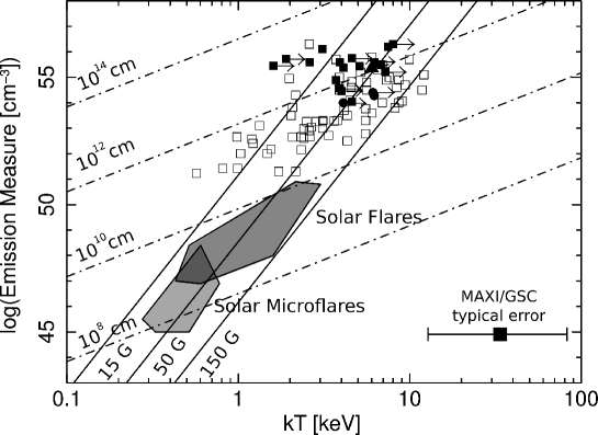
Figure 4: Log-log plot of emission measure ($EM$) vs. plasma temperature ($kT$) for the MAXI X-ray flares (filled symbols, as in figure 2), along with stellar flares from RS-CVn type, Algol, dMe stars and YSOs (open squares; the references given in table 4), solar flares (Feldman et al. (1995)), and solar microflares (Shimizu (1995)). The arrows indicate the lower limits for individual MAXI/GSC sources. The typical error for MAXI/GSC sources in 90% confidence level is indicated at the bottom-right corner.
The three solid lines are the theoretical $EM$-$kT$ relation, based on the equation [$EM\propto B^{-5}T^{17/2}$], for $B$ = 15, 50, and 150 Gauss and the four dashed-dotted lines are that based on the equation [$EM\propto l^{5/3}T^{8/3}$] for the loop-sizes of $10^{8},10^{10}$, $10^{12}$, and $10^{14}$ cm (Shibata & Yokoyama, 1999).

Figure 6: Log-log plot of total energy released radiatively in a flare vs. the square of rotation velocity. The filled symbols are the same as those in figure 2. The open squares, open circles, open triangles, open stars and open circles with a dot show the values obtained in previous studies for RS-CVn type stars, dMe stars, YSOs, dKe stars and the Sun respectively. If flares have been detected from a source with MAXI or the other missions more than once, only the largest $E_{\rm rad}$ is plotted. For the rotation velocity, if the flare source is a multiple-star system, we used the value of the component which has the largest stellar radius.

Table 4: References for figure 4, 5, 6, and 8.

Reference	Figure	Reference	Figure
Alekseev & Kozlova (2001)	6	Montmerle et al. (1983)	4
Amado et al. (2000)	8	Morales et al. (2009)	8
Anders et al. (1999)	6	Morin et al. (2008)	6,8
Benedict et al. (1998)	6	Murdoch et al. (1995)	8
Bopp et al. (1989)	8	O’Brien et al. (2001)	6,8
Briggs & Pye (2003)	4	O’Neal et al. (2001)	6,8
Covino et al. (2001)	4,6,8	Osten & Saar (1998)	6
Demory et al. (2009)	6,8	Osten et al. (2007)	5
Dempsey et al. (1993)	6	Osten et al. (2010)	4,5,6,8
Donati (1999)	8	Ottmann & Schmitt (1994)	4
Donati et al. (1997)	6	Ozawa et al. (1999)	4
Doyle et al. (1988)	4	Pallavicini et al. (1990a)	4,5,6,8
Duemmler & Aarum (2001)	6,8	Pallavicini et al. (1990b)	4
Eaton & Henry (2007)	6,8	Pan & Jordan (1995)	4,6,8
Endl et al. (1997)	4,6,8	Pan et al. (1997)	4,5,8
ESA (1997)	5,6	Pandey & Singh (2008)	4,5,6,8
Favata & Schmitt (1999)	4	Pettersen (1980)	6
Favata et al. (2000a)	5	Pettersen (1989)	8
Favata et al. (2000b)	4,6,8	Pizzolato et al. (2003)	6
Favata et al. (2001)	4,6,8	Poletto et al. (1988)	4
Fekel et al. (1999)	6,8	Preibisch et al. (1993)	4
Franciosini et al. (2001)	4,5	Preibisch et al. (1995)	4
Frasca et al. (1997)	6	Pribulla et al. (2001)	6,8
Güdel et al. (1999)	4	Pye & McHardy (1983)	5,6
Güdel et al. (2004)	4,6,8	Qian et al. (2002)	8
Gagne et al. (1995)	4	Ramseyer et al. (1995)	6
Glebocki & Stawikowski (1995)	6	Randich et al. (1993)	6
Gunn et al. (1998)	8	Reiners & Basri (2007)	6
Hamaguchi et al. (2000)	4	Reiners et al. (2009)	6
Hatzes (1995)	6	Robinson et al. (2003)	6
Huensch & Reimers (1995)	4	Sanz-Forcada et al. (2003)	6,8
Hussain et al. (2005)	6	Singh et al. (1995)	6
Imanishi et al. (2001)	4	Stawikowski & Glebocki (1994)	6
Imanishi et al. (2003)	5	Stern et al. (1983)	4
Jeffries & Bedford (1990)	4,6,8	Stern et al. (1992)	5
Kahler et al. (1982)	4,6	Strassmeier et al. (1993)	6
Kamata et al. (1997)	4	Strassmeier et al. (1994)	6,8
Kjurkchieva et al. (2000)	6	Strassmeier & Rice (1998)	6,8
Kovári et al. (2001)	6	Strassmeier & Rice (2003)	6
Kuerster & Schmitt (1996)	4,6,8	Torres & Ribas (2002)	6,8
Landini et al. (1986)	4,8	Tsuboi et al. (1998)	4,5,8
Lim et al. (1987)	8	Tsuboi et al. (2000)	4
Linsky (1991)	5	Tsuru et al. (1989)	4
Linsky et al. (2001)	8	van den Oord et al. (1988)	4,6,8
Maggio et al. (2000)	4,5,6,8	van den Oord & Mewe (1989)	6,8
Mewe et al. (1997)	4	Welty (1995)	6,8
Miranda et al. (2007)	8	White et al. (1994)	8
Mitra-Kraev (2007)	6	Wright et al. (2011)	6,8
Mitra-Kraev (2007)	6	Yang et al. (2008)	6,8
Miura et al. (2008)	5	Zboril et al. (2005)	6,8
Montes et al. (1995)	6

References

- Alekseev & Kozlova (2001) Alekseev, I. Y., & Kozlova, O. V. 2001, Astrophysics, 44, 429
- Amado et al. (2000) Amado, P. J., Doyle, J. G., Byrne, P. B., et al. 2000, A&A, 359, 159
- Anders et al. (1999) Anders, G. J., Coates, D. W., Thompson, K., & Innis, J. L. 1999, MNRAS, 310, 377
- Argiroffi et al. (2011) Argiroffi, C., Flaccomio, E., Bouvier, J., et al. 2011, A&A, 530, A1
- Benedict et al. (1998) Benedict, G. F., McArthur, B., Nelan, E., et al. 1998, AJ, 116, 429
- Berdyugina et al. (1998) Berdyugina, S. V., Jankov, S., Ilyin, I., Tuominen, I., & Fekel, F. C. 1998, A&A, 334, 863
- Bopp et al. (1989) Bopp, B. W., Saar, S. H., Ambruster, C., et al. 1989, ApJ, 339, 1059
- Briggs & Pye (2003) Briggs, K. R., & Pye, J. P. 2003, MNRAS, 345, 714
- Cargill (2004) Cargill , P. J., & Klimchuck, J. A. 2004, ApJ, 605, 911
- Carlos & Popper (1971) Carlos, R. C., & Popper, D. M. 1971, PASP, 83, 504
- Castro-Tirado et al. (1999) Castro-Tirado, A. J., Brandt, S., Lund, N., & Sunyaev, R. 1999, A&A, 347, 927
- Chambliss (1976) Chambliss, C. R. 1976, PASP, 88, 762
- Christe et al. (2008) Christe, S., Hannah, I. G., Krucker, S., McTiernan, J., & Lin, R. P. 2008, ApJ, 677, 1385
- Collier (1982) Collier, A. C. 1982, Ph.D. Thesis,
- Covino et al. (2001) Covino, S., Panzera, M. R., Tagliaferri, G., & Pallavicini, R. 2001, A&A, 371, 973
- Demory et al. (2009) Demory, B.-O., Ségransan, D., Forveille, T., et al. 2009, A&A, 505, 205
- Dempsey et al. (1993) Dempsey, R. C., Bopp, B. W., Henry, G. W., & Hall, D. S. 1993, ApJS, 86, 293
- Donati (1999) Donati, J.-F. 1999, MNRAS, 302, 457
- Donati et al. (1997) Donati, J.-F., Semel, M., Carter, B. D., Rees, D. E., & Collier Cameron, A. 1997, MNRAS, 291, 658
- Doyle et al. (1988) Doyle, J. G., Butler, C. J., Callanan, P. J., et al. 1988, A&A, 191, 79
- Duemmler & Aarum (2001) Duemmler, R., & Aarum, V. 2001, A&A, 370, 974
- Eaton & Henry (2007) Eaton, J. A., & Henry, G. W. 2007, PASP, 119, 259
- Eker et al. (2008) Eker, Z., Ak, N. F., Bilir, S., et al. 2008, MNRAS, 389, 1722
- Endl et al. (1997) Endl, M., Strassmeier, K. G., & Kurster, M. 1997, A&A, 328, 565
- ESA (1997) ESA 1997, ESA Special Publication, 1200,
- Favata & Micela (2003) Favata, F. & Micela, G. 2003, Space Science Reviews, 108, 577
- Favata et al. (2000b) Favata, F., Micela, G., & Reale, F. 2000b, A&A, 354, 1021
- Favata et al. (2001) Favata, F., Micela, G., & Reale, F. 2001, A&A, 375, 485
- Favata et al. (2000a) Favata, F., Reale, F., Micela, G., et al. 2000a, A&A, 353, 987
- Favata & Schmitt (1999) Favata, F., & Schmitt, J. H. M. M. 1999, A&A, 350, 900
- Fekel (1983) Fekel, F. C., Jr. 1983, ApJ, 268, 274
- Fekel et al. (1999) Fekel, F. C., Strassmeier, K. G., Weber, M., & Washuettl, A. 1999, A&AS, 137, 369
- Feldman et al. (1995) Feldman, U., Laming, J. M., & Doschek, G. A. 1995, ApJ, 451, L79
- Franciosini et al. (2001) Franciosini, E., Pallavicini, R., & Tagliaferri, G. 2001, A&A, 375, 196
- Frasca et al. (1997) Frasca, A., Catalano, S., & Mantovani, D. 1997, A&A, 320, 101
- Güdel (2004) Güdel, M. 2004, A&A Rev., 12, 71
- Güdel et al. (2004) Güdel, M., Audard, M., Reale, F., Skinner, S. L., & Linsky, J. L. 2004, A&A, 416, 713
- Güdel et al. (1999) Güdel, M., Linsky, J. L., Brown, A., & Nagase, F. 1999, ApJ, 511, 405
- Güdel et al. (2002) Güdel, M., Audard, M., Skinner, S. L., & Horvath, M. I. 2002, ApJ, 580, L73
- Gagne et al. (1995) Gagne, M., Caillault, J.-P., & Stauffer, J. R. 1995, ApJ, 450, 217
- Getman et al. (2011) Getman, K. V., Broos, P. S., Salter, D. M., Garmire, G. P., & Hogerheijde, M. R. 2011, ApJ, 730, 6