Integer-valued autoregressive models with survival probability driven by a stochastic recurrence equation

Abstract

A new class of integer-valued autoregressive models with dynamic survival probability is proposed. The peculiarity of this class of models lies on the specification of the survival probability through a stochastic recurrence equation. The estimation of the model can be performed by maximum likelihood and the consistency of the estimator is proved in a misspecified model setting. The flexibility of the proposed specification is illustrated in a simulation study. An application to a time series of crime reports is presented. The results show how the dynamic survival probability can enhance both in-sample and out-of-sample performances of integer-valued autoregressive models.

Key words: Count time series, INAR models, score-driven models, time-varying parameters.

1 Introduction

Over the last few years, there has been an increasing interest in modeling and forecasting integer-valued time series. The reason being that many observed time series are not continuous and the use of specific models to take this into account allows us to better describe time series behaviors. One of the most popular models for time series of counts is the Integer-valued Autoregressive (INAR) model of Al-Osh and Alzaid, (1987) and McKenzie, (1988). Its specification is based on the thinning operator ‘$\circ$’ of Steutel and Van Harn, (1979). For a given $N\in\mathbb{N}$ and $\alpha\in(0,1)$, the thinning operator is defined to satisfy $\alpha\circ N=\sum_{i=1}^{N}x_{i}$, where $\{x_{i}\}_{i=1}^{N}$ is a sequence of independent Bernulli random variables with success probability $\alpha$. The thinning operator enables the specification of integer-valued time series models in an autoregressive fashion. In fact, INAR models can be seen as a discrete response version of the well known linear autoregressive model. The first order INAR model is described by the following equation

$$y_{t}=\alpha\circ y_{t-1}+\varepsilon_{t},\;t\in\mathbb{Z},$$ (1)

where $\{\varepsilon_{t}\}_{t\in\mathbb{Z}}$ is an i.i.d. sequence of integer-valued random variables. An appealing feature of the INAR model in (1) is its well known interpretation as a death-birth process. From this interpretation, the coefficient $\alpha$ is also called the survival probability. As in the original formulation of Al-Osh and Alzaid, (1987) and McKenzie, (1988), the error term $\varepsilon_{t}$ is typically assumed to be Poisson distributed. Other distributions have also been considered in the literature as the Poisson imposes equidispersion and this is can be restrictive in practice, see Al-Osh and Aly, (1992) and Jazi et al., (2012). Besides the distribution of the error term, the INAR specification in (1) has been generalized in several directions. Among others, Alzaid and Al-Osh, (1990) and Jin-Guan and Yuan, (1991) extended the first order INAR model to a general order $p$, Kim and Park, (2008) considered a signed thinning operator to handle nonstationary series and Pedeli and Karlis, (2011) introduced a bivariate INAR model.

Real time series data often exhibit changing dynamic behaviors. As a result, employing more flexible specifications for the dynamic component of the model can provide a better description of the underlying behavior of the time series and produce better forecasts. The contribution of this paper is in this direction: we introduce a new class of INAR models with time-varying survival probability. The peculiarity of our approach is that the dynamics of the INAR coefficient is specified through a Stochastic Recurrence Equation (SRE) that is driven by the score of the predictive likelihood. This method allows the survival probability to be updated at each time period using the information provided by past elements of the series. The use of the score to update time-varying parameters has been recently proposed by Creal et al., (2013) and Harvey, (2013). Since then, their Generalized Autoregressive Score (GAS) framework has been successfully employed to develop dynamic models in econometrics and time series analysis, see for instance Salvatierra and Patton, (2015), Harvey and Luati, (2014) and Creal et al., (2011). It is also worth mentioning that many well-known observation-driven models turn out to be GAS models. Examples include the GARCH model of Engle, (1982) and Bollerslev, (1986) and, in the context of integer-valued time series, the Poisson autoregressive model of Davis et al., (2003). For a more detailed discussion see Creal et al., (2013).

In the literature, time variation of the INAR survival probability has also been considered by Zheng et al., (2007) and Zheng and Basawa, (2008). In Zheng et al., (2007) the survival probability is specified as a sequence of i.i.d. random variables. This approach leads to a more flexible class of conditional distributions but, because of the i.i.d. assumption, it does not provide a dynamic specification of the INAR coefficient. Zheng and Basawa, (2008) allows the INAR coefficient to depend on past observations. Their method introduces a dynamic structure and the survival probability is updated using past information as in our approach. However, as we shall see in Section 4, their specification is not able to properly model smooth changes of the survival probability.

The INAR model we propose in this paper should not be interpreted as a Data Generating Processes (DGP) but as a filter to approximate the distribution of a more complex and unknown DGP. The reasoning behind this interpretation is provided by the work of Blasques et al., (2015). In particular, Blasques et al., (2015) show that score-driven time-varying parameters should be employed in a misspecified model setting as they are optimal in reducing the Kullback-Leibler (KL) divergence with respect to an unknown true DGP. In this direction, we illustrate the flexibility of the proposed dynamic specification for the INAR coefficient by means of a simulation study in a misspecified framework. The results illustrate how the model is able to capture complex dynamic behaviors and well approximate the true distribution of different DGPs. Furthermore, we derive some statistical properties of the Maximum Likelihood (ML) estimator: we prove the its consistency in a misspecified setting and show that also the conditional predictive probability mass function (pmf) can be consistently estimated through a plug-in estimator. In particular, the plug-in pmf estimator is shown to converge to a pseudo-true conditional pmf that has the interpretation of minimizing on average the KL divergence with the true conditional pmf of the DGP. These results are useful not only to ensure the reliability of inference but also forecasting. Finally, the practical usefulness of the proposed model is illustrated thorough an application to a real time series dataset of crime reports. The results are promising and show how the dynamic survival probability can enhance both in-sample and out-of-sample performances of INAR models.

The paper is structured as follows. Section 2 introduces the class of models. Section 3 discusses the consistency of ML estimation. Section 4 presents the Monte Carlo simulation experiments. Section 5 illustrates the empirical application. Section 6 concludes.

2 INAR models with score-driven coefficient

2.1 The class of models

In this section, we extend the class of INAR models in (1) by allowing the survival probability $\alpha$ to change over time. The dynamics of the time-varying coefficient $\alpha_{t}$ is specified on the basis of the score framework of Creal et al., (2013) and Harvey, (2013). The GAS-INAR model is described by the following equations

$$y_{t}= \alpha_{t}\circ y_{t-1}+\varepsilon_{t},$$ (2)

$$\operatorname{\text{logit}}\alpha_{t+1}= \omega+\beta\operatorname{\text{logit}}\alpha_{t}+\tau s_{t},$$ (3)

where $\{\varepsilon_{t}\}_{t\in\mathbb{Z}}$ is an i.i.d. sequence of random variables with pmf $p_{e}(x,\xi)$ for $x\in\mathbb{N}$, $\xi\in\Xi\subseteq\mathbb{R}^{k}$, the vector $\theta=(\omega,\beta,\tau,\xi)^{T}$ is a $k+3$ dimensional parameter vector to be estimated and $s_{t}=s_{t}(\alpha_{t},\xi)$ denotes the score of the predictive log-likelihood $\partial\log p(y_{t}|\alpha_{t},y_{t-1},\xi)/\partial\operatorname{\text{logit}}\alpha_{t}$. Note that throughout the paper we consider the convention that the set $\mathbb{N}$ includes also zero. The functional form of the predictive likelihood $p(y_{t}|\alpha_{t},y_{t-1},\xi)$ can be obtained as the convolution between the conditional pmf of $\alpha_{t}\circ y_{t-1}$ and the pmf of the error term $\varepsilon_{t}$, i.e.

$$p(y_{t}|\alpha_{t},y_{t-1},\xi)=\sum_{k=0}^{\min\{y_{t},y_{t-1}\}}p_{b}(k,y_{t-1},\alpha_{t})p_{e}(y_{t}-k,\xi),$$

where $p_{b}(x,y_{t-1},\alpha_{t})$ for $x\in\{0,\dots,y_{t-1}\}$ is the pmf of a Binomial random variable with size $y_{t-1}$ and success probability $\alpha_{t}$. An analytical expression of the score innovation $s_{t}$ can be found in Appendix A.1. The logit link function in the SRE in (3) is considered to ensure that the survival probability $\alpha_{t}$ is between zero and one.

The GAS-INAR model in (2) and (3) retains the interpretation of INAR models as death-birth processes. In particular, the observed number of elements $y_{t}$ alive at time $t$ is given by the sum between the number of surviving elements from time $t-1$ and the new birth elements $\varepsilon_{t}$. In our dynamic specification, each of the elements alive at time $t-1$ has a probability $\alpha_{t}$ of surviving at time $t$. We also note that the proposed model is observation-driven as the dynamic probability $\alpha_{t}$ is driven solely by past observations. The score $s_{t}$ can be seen as the innovation of the dynamic system in (3) as it provides the new information that becomes available at time $t$ observing $y_{t}$. The interpretation of $s_{t}$ as an innovation is further justified by the fact that its conditional expectation $E(s_{t}|y_{t-1},\alpha_{t})$ is equal to zero.

Figure 1: Impact of $y_{t}$ and $y_{t-1}$ on the score innovation $s_{t}$ for different values of the survival probability $\alpha_{t}$. A Poisson distribution with mean equal to five is considered as distribution of the error term $\varepsilon_{t}$.

It is interesting to see how the information obtained observing $y_{t}$ is processed through the score $s_{t}$ to update the survival probability from $\alpha_{t}$ to $\alpha_{t+1}$. Figure 1 describes the impact of $y_{t}$ on $s_{t}$ for different values of $y_{t-1}$ and $\alpha_{t}$. As we can see from the plots, the survival probability $\alpha_{t}$ gets a negative update when $y_{t}$ is small and $y_{t-1}$ is large. This has an intuitive explanation: the information about $\alpha_{t}$ we get observing a small $y_{t}$ after a large $y_{t-1}$ is that the survival probability should be small as otherwise with a large $\alpha_{t}$ we wold expect many elements from time $t-1$ to survive and thus a large $y_{t}$ as well. As a result, $\alpha_{t}$ should get a negative update to discount this information. Similarly, observing a large $y_{t}$ following a large $y_{t-1}$ suggests an high survival probability. Thus, the probability $\alpha_{t}$ should be updated accordingly and get a positive innovation $s_{t}$. Finally, an innovation $s_{t}$ close to zero may be an indication of either a lack of information or that the observed value of $y_{t}$ is compatible with the value $y_{t-1}$ and the current state of the survival probability $\alpha_{t}$. The former case reflects situations when $y_{t-1}$ is zero (or close to zero). This because observing $y_{t}$ provides no information on the survival probability of the elements $y_{t-1}$ as there are no elements alive at $t-1$. On the other hand, the latter case of observing a value $y_{t}$ compatible with $y_{t-1}$ and $\alpha_{t}$ can be seen as the green area that separates the red an the blue areas in Figure 1.

This line of reasoning concerning the direction of the update $s_{t}$ is subject to the current value of $\alpha_{t}$. For instance, in a situation where $\alpha_{t}$ is close to zero perhaps observing a small $y_{t}$ after a large $y_{t-1}$ is exactly what we would expect. Thus the score update $s_{t}$ may be close to zero in this case. This dependence of the score update $s_{t}$ on the current survival probability $\alpha_{t}$ can be noted across the different plots in Figure 1.

It is also worth mentioning that the functional form of the score innovation $s_{t}$ depends on the specification of the pmf of the error term $\varepsilon_{t}$ as the predictive likelihood depends on it. In practice, the pmf $p_{e}(x,\xi)$ can be chosen in such a way to take into account the main features observed in the data. For instance, as we will consider in the application in Section 5, a Negative Binomial distribution may be considered instead of a Poisson when the data suggests overdispersion. Alternatively, a zero inflated Poisson or Negative Binomial distributions may be employed when dealing with time series with a large number of zeros.

2.2 Parameter estimation

The static parameter vector $\theta$ of the GAS-INAR model can be estimated by ML. The log-likelihood function is available in closed form through a prediction error decomposition, namely

$$\hat{L}_{T}(\theta)=\frac{1}{T}\sum_{t=1}^{T}\log p(y_{t}|\hat{\alpha}_{t}(\theta),y_{t-1},\xi).$$

The filtered survival probability $\hat{\alpha}_{t}(\theta)$ is obtained recursively using the observed data $\{y_{t}\}_{t=0}^{T}$ as

$$\operatorname{\text{logit}}\hat{\alpha}_{t+1}(\theta)=\omega+\beta\operatorname{\text{logit}}\hat{\alpha}_{t}(\theta)+\tau s_{t}(\hat{\alpha}_{t}(\theta),\xi),$$ (4)

where the recursion is initialized at a fixed point $\operatorname{\text{logit}}\hat{\alpha}_{0}(\theta)\in\mathbb{R}$. A reasonable choice for the initialization is $\operatorname{\text{logit}}\hat{\alpha}_{0}(\theta)=\omega/(1-\beta)$. That is the unconditional mean $E\text{logit}\alpha_{t}$ implied by the GAS-INAR model under the parametric assumption $\theta$. This follows immediately as the expected value of the score is equal to zero under standard regularity conditions. The ML estimator is finally given by

$$\hat{\theta}_{T}=\operatorname*{arg\,sup}_{\theta\in\Theta}\hat{L}_{T}(\theta),$$ (5)

where $\Theta$ is a compact parameter set contained in $\mathbb{R}\times(-1,1)\times\mathbb{R}\times\Xi$.

The asymptotic stability of the filtered parameter $\operatorname{\text{logit}}\hat{\alpha}_{t}(\theta)$ and the consistency of the ML estimator as well as the predictive distribution are studied in Section 3. Furthermore, in Section 4, a simulation experiment is performed to study the finite sample behavior of the ML estimator and to further confirm its reliability.

2.3 Forecasting

One of the advantages of properly modeling count time series taking into account the discreteness of the data is that it is possible to obtain coherent forecasts of the entire pmf. As shown in Freeland and McCabe, (2004), forecasts $h$ steps ahead are typically available in closed form for INAR models as in (1). The conditional pmf $h$ steps ahead can be obtained by repeated applications of the convolution formula. Similarly, for point forecasts, a closed form expression is available as the conditional expectation $h$ steps ahead is $E(y_{T+h}|y_{T})=\alpha^{h}y_{T}+\mu$, with $\mu=E(\varepsilon_{t})$.

In the following, we illustrate a possible way to obtain $h$ steps ahead forecasts from the GAS-INAR model. A closed form expression for the conditional pmf $h$ steps ahead $p_{T+h}(x)$ is only available for $h=1$. In particular, it is given by

$$p_{T+1}(x)=\sum_{k=0}^{\min\{x,y_{T}\}}p_{b}(k,y_{T},\alpha_{T})p_{e}(x-k).$$

Numerical methods are required to obtain $p_{T+h}(x)$ for $h\geq 2$. A possibility is to approximate $p_{T+h}(x)$ considering the following simulation scheme. First, simulate $B$ realization for $y_{T+h}$, $y_{T+h}^{(i)}$, $i=1,\dots,B$. Then, obtain an approximation of $p_{T+h}(x)$ as $\hat{p}_{T+h}(x)=n_{x}^{h}/B$, where $n_{x}^{h}$ denotes the number of draws $y_{T+h}^{(i)}$, $i=1,\dots,B$, equal to $x$. The simulations of $y_{T+h}^{(i)}$, $i=1,\dots,B$, can be performed considering the following procedure. For $k=1,\dots,h$

1. Simulate $\varepsilon_{k}^{(i)}$ from the distribution $p_{e}(x,\xi)$ and $\alpha_{T+k}^{(i)}\circ y_{T+k-1}^{(i)}$ from a Binomial distribution with size $y_{T+k-1}^{(i)}$ and success probability $\alpha_{T+k}^{(i)}$.

2. Compute $y_{T+k}^{(i)}=\alpha_{T+k}^{(i)}\circ y_{T+k-1}^{(i)}+\varepsilon_{k}^{(i)}$ and update $\alpha_{T+k}^{(i)}$ to $\alpha_{T+k+1}^{(i)}$ using the recursion $\operatorname{\text{logit}}\alpha_{T+k+1}^{(i)}=\omega+\beta\operatorname{\text{logit}}\alpha_{T+k}^{(i)}+\tau s_{t+k}^{(i)}$.

Similarly, point forecasts $h$ steps ahead can be obtained approximating the conditional expectation $E(y_{T+h}|y_{T},\alpha_{t})$ with the sample average $B^{-1}\sum_{i=1}^{B}y_{T+h}^{(i)}$. Alternatively, the sample median of $y_{T+h}^{(i)}$, $i=1,\dots,B$, can be considered to obtain integer forecasts that are coherent with the discreteness of the data, see Freeland and McCabe, (2004).

3 Some statistical properties

In this section, we discuss the reliability of ML estimation. In particular, we show that the static parameter vector as well as the conditional pmf can be consistently estimated. We focus our asymptotic results on the case of model misspecification. As mentioned before, model misspecification is particularly relevant for models with score-driven parameters. This because they should be interpreted as filters to approximate a more complex and unknown true DGP (Blasques et al.,, 2015). The consistency of the ML estimator is therefore obtained with respect to a pseudo-true parameter that has the interpretation of minimizing an average KL divergence between the GAS-INAR model and an unknown true DGP. Consistency arguments with respect to pseudo-true parameters go back to White, (1982). In the following, we shall only assume that the observed data are generated by a stationary and ergodic count process without imposing a specific DGP.

3.1 Stability of the filter

A key ingredient to ensure the reliability of the ML estimator for observation-driven models is the stability of the filtered time-varying parameter. The stability of the filter is typically referred in the literature as the invertibility of the model, see Straumann and Mikosch, (2006) and Wintenberger, (2013). As a first step, we derive conditions to ensure that the filtered parameter in (4) converges to a unique stationary sequence irrespective of the initialization $\hat{\alpha}_{0}(\theta)$. This result is particularly important as it implies that the initialization is irrelevant asymptotically and provides the basis to ensure the consistency of the ML estimator.

First, we impose some regularity conditions on the pmf of the error term $p_{e}(x,\xi)$.

Assumption 3.1.

The function $\xi\mapsto p_{e}(x,\xi)$ is continuous in $\Xi$ for any $x\in\mathbb{N}$ and $p_{e}(x,\xi)>0$ for any $(x,\xi)\in\mathbb{N}\times\Xi$.

Assumption 3.1 requires the pmf $p_{e}(x,\xi)$ to have full support in $\mathbb{N}$ and to be continuous with respect to $\xi$. These conditions are satisfied for most parametric pmf such as the Poisson, the zero inflated Poisson and the Negative Binomial. However, it is worth mentioning that distributions with limited support such as the Binomial are ruled out by this assumption.

The next result ensures the stability of the filtered parameter $\{\hat{\alpha}_{t}(\theta)\}_{t\in\mathbb{N}}$ specified in (4). In particular, it shows the exponential almost sure (e.a.s.) uniform convergence of the functional sequence $\{\hat{\alpha}_{t}\}_{t\in\mathbb{N}}$ to a unique stationary and ergodic functional sequence $\{\tilde{\alpha}_{t}\}_{t\in\mathbb{Z}}$. The convergence is considered with respect to the uniform norm $\|\cdot\|_{\Theta}$, where $\|f\|_{\Theta}=\sup_{\theta\in\Theta}|f(\theta)|$ for any function $f$ that maps from $\Theta$ into $\mathbb{R}$. We recall that a sequence of non-negative random variables $\{w_{t}\}_{t\in\mathbb{N}}$ is said to converge e.a.s. to zero if there exists a constant $\gamma>1$ such that $\gamma^{t}w_{t}\xrightarrow{a.s.}$ 0 as $t$ diverges.

Proposition 3.1.

Assume that $\{y_{t}\}_{t\in\mathbb{Z}}$ is a stationary and ergodic sequence of count random variables such that $Ey_{t}^{2}<\infty$. Moreover, let Assumption 3.1 be satisfied and let the following condition hold

$$E\log\sup_{\alpha\in(0,1)}|\beta+\tau\dot{s}_{t}(\alpha,\xi)|<0,\;\;\forall\;\theta\in\Theta,$$ (6)

where $\dot{s}_{t}(\alpha,\xi)=\partial s_{t}(\alpha,\xi)/\partial\operatorname{\text{logit}}\alpha$. Then, the filtered parameter $\{\hat{\alpha}_{t}(\theta)\}_{t\in\mathbb{N}}$ defined in (4) converges e.a.s. and uniformly in $\Theta$ to a unique stationary and ergodic sequence $\{\tilde{\alpha}_{t}(\theta)\}_{t\in\mathbb{Z}}$, i.e.

$$\|\operatorname{\text{logit}}\hat{\alpha}_{t}-\operatorname{\text{logit}}\tilde{\alpha}_{t}\|_{\Theta}\xrightarrow{\text{e.a.s.}}0\;\;\text{as}\;\;t\rightarrow\infty,$$

for any initialization $\hat{\alpha}_{0}$ of the filter.

The proof is given in the appendix. Proposition 3.1 does not require correct specification of the model. The observed data can be generated by any stationary and ergodic count process.

The contraction condition in (6) can be checked empirically using the observed data. It is not possible to obtain a closed form expression for (6) as it depends on the DGP and on the specification of $p_{e}(x,\xi)$. However, with the next proposition, we show that the parameter region $\Theta$ that satisfies (6) is not degenerate.

Proposition 3.2.

The contraction condition $(\ref{contraction})$ of Proposition 3.1 is implied by the following sufficient condition

$$E\log\max(|\beta-\tau y_{t-1}/4|,|\beta+\tau m_{t}^{2}|)<0,\;\;\forall\;\theta\in\Theta,$$

where $m_{t}=\min\{y_{t-1},y_{t}\}$.

Proposition 3.2 guarantees that the parameter region $\Theta$ is not degenerate as for small enough $|\beta|$ and $|\tau|$ the inequality is always satisfied.

3.2 Consistency of ML estimation

We assume the observed data to be a realized path from an unknown DGP $\{y_{t}\}_{t\in\mathbb{Z}}$. Furthermore, we denote with $p^{o}(x|y^{t-1})$, $x\in\mathbb{N}$, the true pmf of $y_{t}$ conditionally on the past observations $y^{t-1}=\{y_{t-1},y_{t-2},\dots\}$. The KL divergence between the true conditional pmf $p^{o}(x|y^{t-1})$ and the postulated pmf $p(x|\tilde{\alpha}_{t}(\theta),y_{t-1},\xi)$ is given by

$$KL_{t}(\theta)=\sum_{x=0}^{\infty}\log\left(\frac{p^{o}(x|y^{t-1})}{p(x|\tilde{\alpha}_{t}(\theta),y_{t-1},\xi)}\right)p^{o}(x|y^{t-1}).$$

Note that conditional KL divergence $KL_{t}(\theta)$ depends on $t$ as it is a function of the past observations $y^{t-1}$. We are now ready to formally define the pseudo-true parameter $\theta^{*}$.

Definition 3.1.

The pseudo-true parameter $\theta^{*}$ is the minimizer of the average KL divergence $KL(\theta)={E}KL_{t}(\theta)$ in the parameter set $\Theta$.

We also denote with $\alpha_{t}^{*}=\tilde{\alpha}_{t}(\theta^{*})$ the pseudo-true dynamic survival probability and with $p_{t}^{*}(x)=p(x|\alpha_{t}^{*},y_{t-1},\xi^{*})$, $x\in\mathbb{N}$, the pseudo-true conditional pmf. In the following, we also prove the consistency of the plug-in estimators $\hat{\alpha}_{t}(\hat{\theta}_{T})$ and $\hat{p}_{t}(x,\hat{\theta}_{T})=p(x|y_{t-1},\hat{\alpha}_{t}(\hat{\theta}_{T}),\hat{\xi}_{T})$ for the time-varying survival probability and conditional pmf respectively. This is of practical interest as typically the main objective of INAR models is not the interpretation of the static parameter estimates but approximating the true pmf for forecasting purposes.

We start considering the following assumption, which imposes some moment conditions and the contraction condition of Proposition 3.1.

Assumption 3.2.

The following moment conditions hold true $Ey^{2}_{t}<\infty$, $E|\log p^{o}(y_{t}|y^{t-1})|<\infty$ and $E\sup_{\theta\in\Theta}|\log p_{e}(y_{t},\xi)|<\infty$. Furthermore, the contraction condition in (6) is satisfied.

Assumption 3.2 is needed to ensure the uniform a.s. convergence of the likelihood function $\hat{L}_{T}(\theta)$ to a well defined deterministic function $L(\theta)=El_{0}(\theta)$, where $l_{t}(\theta)=\log p(y_{t}|\tilde{\alpha}_{t}(\theta),y_{t-1},\xi)$ denotes the $t$-th contribution to the likelihood function when the limit filter $\tilde{\alpha}_{t}(\theta)$ is considered. Furthermore, the integrability condition on the unknown true pmf $E|\log p^{o}(y_{t}|y^{t-1})|<\infty$ is required to ensure that the average KL divergence exists and thus the maximizer of $L(\theta)$ corresponds to the pseudo-true parameter $\theta^{*}$.

Note also that the uniform moment condition $E\sup_{\theta\in\Theta}|\log p_{e}(y_{t},\xi)|<\infty$ is needed only because we are considering a general class of pmf for the error term. For most pmf, this condition is always satisfied. For instance, it holds true immediately as long as $Ey_{t}^{2}<\infty$ if $p_{e}(x,\xi)$ is a Poisson or a Negative Binomial pmf.

Finally, we impose the following identifiability condition.

Assumption 3.3.

The function $L(\theta)=El_{0}(\theta)$ has a unique maximizer in the set $\Theta$.

Assumption 3.3 ensures the uniqueness of the pseudo-true parameter $\theta^{*}$. In general, if this assumption is not satisfied, we obtain that the limit points of the ML estimator belong to the set of points that minimize the average KL divergence $KL(\theta)$.

We are now ready to deliver the strong consistency of the ML estimator with respect to the pseudo-true parameter $\theta^{*}$.

Theorem 3.1.

Let the observed data $\{y_{t}\}_{t=1}^{T}$ be generated by a stationary and ergodic count process $\{y_{t}\}_{t\in\mathbb{Z}}$ and let the assumptions 3.1-3.3 be satisfied. Then the ML estimator defined in (5) is strongly consistent with respect to the pseudo-true parameter $\theta^{*}$, i.e.

$$\hat{\theta}_{T}\xrightarrow{\text{a.s.}}\theta^{*},\;\;\;\;T\xrightarrow{}\infty.$$

As special case of Theorem 3.1, we could also obtain the strong consistency of the ML estimator when the model is correctly specified.

Remark 3.1.

If we assume that the observed data $\{y_{t}\}_{t=1}^{T}$ are generated by a stationary and ergodic process $\{y_{t}\}_{t\in\mathbb{Z}}$ that satisfies the model’s equations (2) and (3) for $\theta=\theta_{0}$, $\theta_{0}\in\Theta$. It can be easily shown that under Assumptions 3.1-3.3 the ML estimator is strongly consistent.

In the next section, the finite sample properties of the ML estimator under correct specification are investigated through a simulation study.

We now turn our attention to the study of the consistency of the plug-in estimators $\hat{\alpha}_{t}(\hat{\theta}_{T})$ and $\hat{p}_{t}(x,\hat{\theta}_{T})$. Note that the consistency of these estimators do not follow trivially from the consistency of $\hat{\theta}_{T}$. This because these plug-in estimators are random functions of $\hat{\theta}_{T}$ that change at different time $t$ without converging. Therefore, it is not possible to trivially apply a continuous mapping theorem and immediately obtain the desired consistency. The results we obtain require that both $t$ and the sample size $T$ go to infinity. This because $T\rightarrow\infty$ is needed for the consistency of the ML estimator and $t\rightarrow\infty$ is needed to make the effect of the initialization of the filter to vanish.

The next result shows that the plug-in estimator $\hat{\alpha}_{t}(\hat{\theta}_{T})$ is strongly consistent with respect to the pseudo-true survival probability $\alpha_{t}^{*}$.

Lemma 3.1.

Let the conditions of Theorem 3.1 hold. Then, the plug-in estimator $\operatorname{\text{logit}}\hat{\alpha}_{t}(\hat{\theta}_{T})$ is strongly consistent, i.e.

$$\left|\operatorname{\text{logit}}\hat{\alpha}_{t}(\hat{\theta}_{T})-\operatorname{\text{logit}}\alpha_{t}^{*}\right|\xrightarrow{\text{a.s.}}0,\;\;\;\;\;\;t\xrightarrow{}\infty,\;T\xrightarrow{}\infty.$$

In order to obtain the consistency of the plug-in estimator $\hat{p}_{t}(x,\hat{\theta}_{T})$, we need the following additional regularity condition on the pmf of the error term.

Assumption 3.4.

The function $\xi\mapsto p_{e}(x,\xi)$ is continuously differentiable in $\Xi$ for any $x\in\mathbb{N}$.

Assumption 3.4 is a standard regularity condition that is satisfied for most popular pmf such as the Poisson and the Negative Binomial. The next result delivers the consistency of the conditional pmf estimator. In this case, we are only able to ensure consistency and not strong consistency.

Theorem 3.2.

Let the observed data $\{y_{t}\}_{t=1}^{T}$ be generated by a stationary and ergodic count process $\{y_{t}\}_{t\in\mathbb{Z}}$ and let the assumptions 3.1-3.4 be satisfied. Then the conditional pmf plug-in estimator $\hat{p}_{t}(x,\hat{\theta}_{T})$ is consistent, i.e.

$$|\hat{p}_{t}(x,\hat{\theta}_{T})-p^{*}_{t}(x)|\xrightarrow{\text{pr.}}0,\;\;\;\;\;t\xrightarrow{}\infty,\;T\xrightarrow{}\infty,$$

for any $x\in\mathbb{N}$.

4 Monte Carlo experiment

4.1 Finite sample behavior of the ML estimator

We first perform a Monte Carlo simulation experiment to test the reliability of the ML estimator in finite samples. We consider the dynamic INAR model specified in (2) and (3) with a Poisson error distribution having mean $\mu$. The experiment consists on generating $1000$ time series of size $T$ from the GAS-INAR model and estimating the parameter vector $\theta=(\omega,\beta,\tau,\mu)^{T}$ by maximum likelihood. Different parameter values $\theta$ and different sample sizes $T$ are considered. The simulation results are collected in Table 1. In particular, Table 1 reports the mean, the bias, the Standard Deviation (SD) and the square root of the Mean Squared Error (MSE) of the ML estimator obtained from the $1000$ Monte Carlo replications.

		$\omega$	$\beta$	$\tau$	$\mu$		$\omega$	$\beta$	$\tau$	$\mu$
True Value		-0.50	0.90	0.15	6.00		-0.50	0.95	0.15	6.00
$T=250$	Mean	-0.505	0.825	0.161	5.985		-0.496	0.896	0.159	5.996
	Bias	-0.005	-0.075	0.011	-0.015		0.004	-0.054	0.009	-0.004
	SD	0.326	0.175	0.100	0.588		0.411	0.117	0.097	0.570
	$\sqrt{\text{MSE}}$	0.326	0.190	0.101	0.588		0.411	0.129	0.097	0.570
$T=500$	Mean	-0.496	0.868	0.153	5.986		-0.503	0.927	0.154	5.997
	Bias	0.004	-0.032	0.003	-0.014		-0.003	-0.023	0.004	-0.003
	SD	0.213	0.093	0.062	0.407		0.246	0.053	0.053	0.393
	$\sqrt{\text{MSE}}$	0.213	0.098	0.062	0.407		0.246	0.058	0.053	0.392
$T=1000$	Mean	-0.494	0.885	0.151	5.987		-0.499	0.939	0.150	5.992
	Bias	-0.006	-0.015	0.001	-0.013		-0.001	-0.011	0.000	-0.008
	SD	0.152	0.050	0.042	0.295		0.171	0.034	0.035	0.279
	$\sqrt{\text{MSE}}$	0.152	0.052	0.042	0.295		0.171	0.036	0.035	0.279
True Value		-0.50	0.90	0.30	6.00		-0.50	0.95	0.30	6.00
$T=250$	Mean	-0.481	0.862	0.304	5.943		-0.502	0.916	0.302	5.945
	Bias	0.019	-0.038	0.004	-0.057		-0.002	-0.034	0.002	-0.055
	SD	0.361	0.095	0.101	0.512		0.501	0.066	0.097	0.473
	$\sqrt{\text{MSE}}$	0.361	0.103	0.101	0.514		0.500	0.075	0.097	0.476
$T=500$	Mean	-0.495	0.883	0.297	5.971		-0.492	0.935	0.298	5.971
	Bias	0.005	-0.017	-0.003	-0.029		0.008	-0.015	-0.002	-0.055
	SD	0.221	0.044	0.057	0.338		0.361	0.030	0.052	0.310
	$\sqrt{\text{MSE}}$	0.221	0.048	0.057	0.339		0.361	0.033	0.052	0.311
$T=1000$	Mean	-0.490	0.891	0.299	5.978		-0.502	0.943	0.298	5.981
	Bias	0.010	-0.019	-0.001	-0.022		-0.002	-0.007	0.002	-0.019
	SD	0.156	0.029	0.040	0.242		0.233	0.019	0.035	0.219
	$\sqrt{\text{MSE}}$	0.156	0.031	0.040	0.243		0.233	0.020	0.035	0.220

Table 1: Summary statistics of the sample ML estimator distribution for different parameter values $\theta$ and different sample sizes $T$. The statistics in the table are obtained from 1000 Monte Carlo replications.

The simulation results in Table 1 further suggest that the parameter vector $\theta$ can be consistently estimated by maximum likelihood. This can be elicited from the fact that the MSE of the estimator is decreasing as the sample size $T$ increases. We also note that the estimator of the parameter $\beta$ tends to be negatively biased in finite samples. In all the cases considered, the parameter $\beta$ is underestimated on average. The magnitude of the bias seems also to be relevant as, especially for $T=250$, the square root of the MSE is considerably larger then the SD. Therefore, this indicates that the bias contribution to the MSE is not negligible compared to the variance contribution. The negative bias for $\beta$ is not surprising as the values of $\beta$ considered in the simulations are close to 1 and similar results on the bias are well known for ML estimation of linear autoregressive models. As concerns the other parameters, the results suggest that the bias can be considered negligible as the SD is almost equal to the square root of the MSE in all the scenario considered.

4.2 Filtering under misspecification

Score-driven updates for time-varying parameters have been shown to be optimal in a misspecified framework where the aim is to reduce the KL divergence between the postulated model and the true unknown DGP, see Blasques et al., (2015). This section illustrates the flexibility of the proposed GAS-INAR specification through a simulation study. In this experiment, we consider different DGPs of the form

$$y_{t}=\alpha^{o}_{t}\circ y_{t-1}+\varepsilon_{t},\;\;\;\varepsilon_{t}\sim\mathcal{P}(5),$$

where $\mathcal{P}(5)$ denotes a Poisson distribution with mean equal to 5. The DGPs differ on the basis of the specification of the sequence $\{\alpha_{t}^{o}\}_{t\in\mathbb{Z}}$. The following four dynamics are considered.

1. Fast sine: $\alpha_{t}^{o}=0.5+0.25\sin(\pi t/100)$.

2. Slow sine: $\alpha_{t}^{o}=0.5+0.25\sin(\pi t/250)$.

3. Fast steps: $\alpha_{t}^{o}=0.25I_{[-1,0]}\left(\sin(\pi t/100)\right)+0.75I_{(0,1]}\left(\sin(\pi t/100)\right)$.

4. Slow steps: $\alpha_{t}^{o}=0.25I_{[-1,0]}\left(\sin(\pi t/250)\right)+0.75I_{(0,1]}\left(\sin(\pi t/250)\right)$.

where $I_{A}(x)=1$ if $x\in A$ and $I_{A}(x)=0$ otherwise. The DGPs are thus Poisson INAR models where the coefficient $\alpha_{t}^{o}$ is allowed to change in different ways. The red lines in Figure 2 show the path of $\alpha_{t}^{o}$, $t=1,\dots,500$, for the four different DGPs. As we can see, the fast sine and the slow sine specifications allow the coefficient to change smoothly over time, whereas, the fast step and slow step specifications exhibit abrupt changes over time.

	Square root MSE
	Fast sine	Slow sine	Fast steps	Slow steps
INAR	0.242	0.257	0.322	0.356
rc-INAR	0.112	0.111	0.145	0.132
GAS-INAR	0.077	0.060	0.101	0.072
	KL divergence
	Fast sine	Slow sine	Fast steps	Slow steps
INAR	0.238	0.253	0.412	0.442
rc-INAR	0.117	0.114	0.212	0.185
GAS-INAR	0.053	0.029	0.128	0.057

Table 2: Average MSE and KL divergence between the true DGP and the different models.

Figure 2: The red line denotes the true path $\alpha_{t}^{o}$. The gray area represents confidence bounds of the filtered path of $\alpha_{t}$ for the GAS-INAR model. The first plot is for the fast sine configuration, the second is for the slow sine, the third is for the fast steps and the last is for the slow steps specification.

The simulation experiment consists on generating $1000$ Monte Carlo time series draws of size $T=500$ from the different DGPs. For each draw, the following models are estimated: a Poisson INAR model with static coefficient, the GAS-INAR model with Poisson error terms and a Poisson INAR model with dynamic coefficient as considered in Zheng and Basawa, (2008). For the latter model the dynamic survival probability is given by $\operatorname{\text{logit}}\alpha_{t}=\omega+\tau y_{t-1}$, where $\omega$ and $\tau$ are parameters to be estimated. The model of Zheng and Basawa, (2008) is denoted as rc-INAR. The performances of the models is measured in terms of approximation of the true conditional pmf and the true survival probability $\alpha_{t}^{o}$. As concerns pmf approximation, we compute the KL divergence between the true pmf and the estimated one. Whereas, as concerns $\alpha_{t}^{o}$, we consider the MSE between $\alpha_{t}^{o}$ and the estimated survival probability. Table 2 reports the results of the simulation experiment. As we can see, the GAS-INAR model has the pest performance in terms of both KL divergence and MSE. This is true for all the DGPs considered. We also note that the better performance of the GAS-INAR model is relevant in relative terms. In particular, the KL divergence and MSE from the GAS-INAR model are about half of those from the rc-INAR model and about one third of those from the INAR model. These results show the flexibility of the GAS-INAR model and its ability to approximate complex DGPs.

Figure 2 further illustrates the ability of the GAS-INAR specification to capture the dynamic behavior of the true $\alpha_{t}^{o}$ in the different settings considered. The gray areas in the plots represent $95\%$ variability bounds for the estimated paths of $\alpha_{t}$ and the red lines denote the true paths $\alpha_{t}^{o}$. As we can see, in the fast sine and slow sine configurations, the true path $\alpha_{t}^{o}$ is always inside the $95\%$ confidence bounds. This shows the ability of the GAS-INAR model to capture smooth changes in $\alpha_{t}^{o}$. On the other hand, in the fast steps and slow steps configurations, the true $\alpha_{t}^{o}$ is not inside the confidence bounds right after the sudden changes in the level of $\alpha_{t}^{o}$. This is natural as the filtered path requires some time periods before adapting to the break in the level of $\alpha_{t}^{o}$. However, also in this situation, we can see how the estimated paths from the GAS-INAR model are able to approximate reasonably well the true $\alpha_{t}^{o}$.

5 Application to crime data

5.1 In-sample results

We present an empirical illustration of the proposed methodology to the monthly number of offensive conduct reports in the city of Blacktown, Australia, from January 1995 to December 2014. The time series is from the New South Wales dataset of police reports and it is available at http://data.gov.au/.

Figure 3: The first plot shows the monthly number of offensive conduct reports in Blacktown from January 1995 to December 2014. The second and third plots represent the sample autocorrelation functions of the series.

Figure 3 shows the plot of the series. As we can see, there are two time periods with a particular high level of criminal activities. The first is around 2002 and the second is around 2010. During these periods we expect the estimated survival probability $\alpha_{t}$ to be higher as they can be seen as periods of high persistence. As discussed in Jin-Guan and Yuan, (1991), INAR(p) models have the same autocorrelation structure of continuous-valued AR(p) models. The sample autocorrelation functions in Figure 3 suggest that a first-order INAR model should be appropriate for this dataset. We consider several model specifications: the INAR and the GAS-INAR model with Poisson and Negative Binomial error distribution. The sample mean of the data is $9.3$ and the sample variance is $24.3$. This is an indication that there is overdispersion in the data and thus a Negative Binomial distribution for the error term may be more suited. The different specifications employed are summarized in Table 3.

	Model description
GAS-NBINAR	Model in (2) and (3) with Negative Binomial error of mean $\mu$ and variance $\sigma^{2}$.
NBINAR	Model in (1) with Negative Binomial error of mean $\mu$ and variance $\sigma^{2}$.
GAS-PoINAR	Model in (2) and (3) with Poisson error of mean $\mu$.
PoINAR	Model in (1) with Poisson error of mean $\mu$.

Table 3: The table describes the specification of each model.

	$\omega$	$\beta$	$\tau$	$\mu$	$\sigma^{2}$	log-lik	pvalue	AIC
GAS-NBINAR	-0.907	0.965	0.135	6.083	14.155	-662.91	0.002	1335.82
	(0.338)	(0.027)	(0.055)	(0.481)	(1.853)
NBINAR	-0.401	-	-	5.586	15.265	-669.03	-	1344.07
	(0.176)			(0.456)	(2.125)
GAS-PoINAR	-1.258	0.967	0.141	6.539	-	-695.04	0.000	1398.24
	(0.294)	(0.019)	(0.033)	(0.313)
PoINAR	-0.613	-	-	6.046	-	-714.58	-	1433.21
	(0.140)			(0.323)

Table 4: ML estimate of the models in Table 3. The last three columns contain respectively the log-likelihood, the pvalue of the likelihood ratio test between the GAS-INAR models and their static INAR counterparts and the AIC.

The ML estimation results are collected in Table 4. We consider the likelihood ratio test to check the significance of the dynamic coefficient $\alpha_{t}$. Given its meaningful interpretation in a misspecified framework, we also report the Akaike Information Criterion (AIC) as a means of comparison among non-nested models. The results suggest that the inclusion of the dynamic specification for $\alpha_{t}$ plays a relevant role as confirmed by the likelihood ratio test and the AIC. The likelihood ratio test shows that the dynamic coefficient is highly significant for both the Poisson and the Negative Binomial specifications. Overall the model with the smallest AIC is the GAS-NBINAR model. Furthermore, for both the Negative Binomial models, the estimated variance of the error term is more than double the estimated mean. We can thus say that the Negative Binomial distribution seems to provide a better fitting than the Poisson. This result is also coherent with the overdispersion observed in the data. We can conclude that the results indicate a better in-sample performance for the GAS-INAR model.

From Table 4, we also note that the time-varying parameter $\alpha_{t}$ is highly persistent as the estimated $\beta$ is close to 1. The estimated path of $\alpha_{t}$ together with $80\%$ and $95\%$ confidence bounds is plotted in Figure 4. As expected, the survival probability is particularly high around 2002 and around 2010. This reflects the high level of criminal activities that can be interpreted as an higher survival probability of past elements. The plot in Figure 4 also highlights that there is a relevant difference in considering a static $\alpha$ instead of a dynamic $\alpha_{t}$. This can be noted from the fact that the dashed line, which denotes the static parameter estimate of $\alpha$, lies outside the 95% confidence bounds of $\alpha_{t}$ in some time periods.

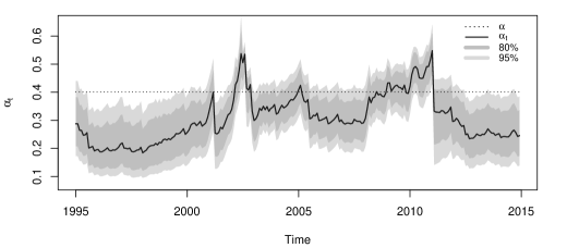
Figure 4: Estimated $\alpha_{t}$ from the GAS-NBINAR model with 80% and 95% confidence bounds. The dashed line represents the estimate of $\alpha$ from the NBINAR model. The confidence bounds are obtained simulating from the distribution of the ML estimator as proposed by Blasques et al., (2016).

5.2 Forecasting results

Finally we perform a pseudo out-of-sample experiment to compare the forecasting performances of the models. The full sample size of the series is 240 observations. We split it into two subsamples: the first 140 observations are considered as a training sample and the last 100 observations as a forecasting evaluation sample. The training sample is then expanded recursively. We evaluate the forecast performance of the models in terms of both point forecast and pmf forecast. The point forecast accuracy is evaluated by the forecast MSE, i.e. $100^{-1}\sum_{i=1}^{100}(\hat{y}_{T+i}-y_{T+i})^{2}$. Whereas, the pmf forecast accuracy is evaluated by the log score criterion, i.e. $100^{-1}\sum_{i=1}^{100}\log\hat{p}_{T+i}(y_{T+i})$. The log score criterion provides a means of comparison based on the KL divergence between the true DGP and the estimated models.

	Mean squared error
	$h=1$	$h=2$	$h=3$	$h=4$	$h=5$	$h=6$
GAS-NBINAR	15.77	20.15	20.56	21.51	21.36	21.23
NBINAR	16.51	21.47	22.61	23.70	23.85	23.72
GAS-PoINAR	16.33	20.66	21.18	21.98	21.82	21.52
PoINAR	17.00	21.82	22.86	23.79	23.91	23.78
	Log score criterion
	$h=1$	$h=2$	$h=3$	$h=4$	$h=5$	$h=6$
GAS-NBINAR	-2.73	-2.82	-2.83	-2.85	-2.85	-2.85
NBINAR	-2.75	-2.85	-2.88	-2.91	-2.91	-2.91
GAS-PoINAR	-2.83	-2.96	-2.98	-3.00	-3.00	-2.98
PoINAR	-2.88	-3.08	-3.12	-3.18	-3.19	-3.18

Table 5: Forecast MSE and log score criterion computed in the last 100 observations for different forecast horizons.

The results are collected in Table 5. As we can see, the inclusion of the dynamic survival probability $\alpha_{t}$ provides better forecast performances in the subsample considered. In particular, the GAS-NBINAR model outperforms the NBINAR model in terms of both point forecasts and pmf forecasts. The same happens for the GAS-PoINAR compared to the PoINAR. This holds true for all forecast horizons considered. Furthermore, the use of the Negative Binomial distribution is particularly relevant to improve the pmf forecasts. In particular, the Negative Binomial models dominate the Poisson models in terms of log-score criterion. This result is quite natural as the the Negative Binomial models take into account the overdispersion in the data. On the other hand, as concerns the point forecasts, the dynamic parameter $\alpha_{t}$ seems to play a mayor role in improving the forecast performances. This can be noted as the models with dynamic $\alpha_{t}$ dominate the models with static $\alpha$ in terms on MSE. The best performing model is the GAS-NBINAR for both criteria and all forecast horizons. This suggests that the flexibility introduced by $\alpha_{t}$ as well as the choice of an appropriate distribution for the error term can be important to better predict future observations. Overall, these out-of-sample results together with the in-sample results show that the GAS-INAR models can be useful in practical applications.

6 Conclusion

In this paper, we have proposed a flexible INAR model with dynamic survival probability. This model should be interpreted as a filter to approximate unknown DGPs. Empirical results are promising as illustrated in the empirical experiments considering both simulated data and real data. Future research may include the extension of the first-order dynamic INAR model to a general order $p$. Other work to be done concerns the asymptotic theory of the ML estimator. At the moment, we have only proved the consistency of the estimator. The asymptotic normality requires the study of the first two derivatives of the log likelihood. In this regard, we encountered some difficulties concerning the existence of some moments for the derivative processes.

Appendix A Appendix

A.1 Derivatives of the predictive log-likelihood

Defining $s_{t}(\alpha,\xi):=\partial\log p(y_{t}|\alpha,y_{t-1},\xi)/\partial\operatorname{\text{logit}}\alpha$ and $\dot{s}_{t}(\alpha,\xi):=\partial s_{t}(\alpha,\xi)/\partial\operatorname{\text{logit}}\alpha$, by elementary calculus, we obtain that

$$s_{t}(\alpha,\xi)=\left(\sum_{k=0}^{m_{t}}p_{kt}(\alpha,\xi)\right)^{-1}\left(\sum_{k=0}^{m_{t}}p_{kt}(\alpha,\xi)(k-y_{t-1}\alpha)\right),$$ (7)

and

$$\dot{s}_{t}(\alpha,\xi)= \left(\sum_{j=0}^{m_{t}}\sum_{k=0}^{m_{t}}p_{kt}(\alpha,\xi)p_{jt}(\alpha,\xi)\right)^{-1}\times$$

$$\qquad\left(\sum_{j=0}^{m_{t}}\sum_{k=0}^{m_{t}}p_{kt}(\alpha,\xi)p_{jt}(\alpha,\xi)\left(k(k-j)-\alpha(1-\alpha)y_{t-1}\right)\right),$$ (8)

where $m_{t}=\min(y_{t},y_{t-1})$ and

$$p_{kt}(\alpha,\xi)={y_{t-1}\choose k}\alpha^{k}(1-\alpha)^{y_{t-1}-k}p_{e}(y_{t}-k,\xi).$$

A.2 Proofs

Proof of Proposition 3.1.

The stability conditions we consider to obtain the convergence result are based on Theorem 3.1 of Bougerol, (1993). Straumann and Mikosch, (2006) applied Bougerol’s theorem in the space of continuous functions $\mathbb{C}(\Theta,\mathbb{R})$ equipped with the uniform norm $\|\cdot\|_{\Theta}$. In particular, they provide stability conditions for functional SRE of the form

$$x_{t+1}(\theta)=\phi_{t}(x_{t}(\theta),\theta),\;t\in\mathbb{N},$$ (9)

where $x_{0}(\theta)\in\mathbb{R}$, the map $(x,\theta)\mapsto\phi_{t}(x,\theta)$ from $\mathbb{R}\times\Theta$ into $\mathbb{R}$ is almost surely continuous and the sequence $\{\phi_{t}(x,\theta)\}_{t\in\mathbb{Z}}$ is stationary and ergodic for any $(x,\theta)\in\mathbb{R}\times\Theta$. Wintenberger, (2013) weakened Straumann and Mikosch, (2006) conditions replacing a uniform contraction condition with a pointwise condition. The uniform e.a.s convergence of a filter satisfying the SRE in (9) can be obtained on the basis of Theorem 2 of Wintenberger, (2013) from the following conditions:

(a)

There exists an $x\in\mathbb{R}$ such that $E\log^{+}\left(\sup_{\theta\in\Theta}|\phi_{0}(x,\theta)|\right)<\infty$,

(b)

$E\log^{+}\left(\sup_{\theta\in\Theta}\Lambda_{0}(\theta)\right)<\infty$,

(c)

$E\log\left(\Lambda_{0}(\theta)\right)<0$ for any $\theta\in\Theta$,

where the random coefficient $\Lambda_{t}(\theta)$ is defined as

$$\Lambda_{t}(\theta)=\sup_{(x_{1},x_{2})\in\mathbb{R}^{2},x_{1}\neq x_{2}}\frac{|\phi_{t}(x_{1},\theta)-\phi_{t}(x_{2},\theta)|}{|x_{1}-x_{2}|}.$$

In our case, the random function $\phi_{t}$ that defines the SRE in (9) has the following form

$$\phi_{t}(x,\theta)=\omega+\beta x+\tau s_{t}\left(\operatorname{\text{logit}}^{-1}(x),\xi\right).$$

First we note that our SRE satisfies the stationarity and continuity requirements to apply Wintenberger’s results. In particular, we obtain that the a.s. continuity of $\phi_{t}(x,\theta)$ follows immediately from the a.s. continuity of $(x,\theta)\mapsto s_{t}\left(\operatorname{\text{logit}}^{-1}(x),\xi\right)$, which is implied by Assumption 3.1, and the continuity of the Binomial likelihood (see the functional form of $s_{t}$ in (7)). Furthermore, the stationarity and ergodicity of $\{\phi_{t}\}_{t\in\mathbb{Z}}$ follows from the stationarity and ergodicity of $\{y_{t}\}_{t\in\mathbb{Z}}$ together with an application of Proposition 4.3 of Krengel, (1985) as $s_{t}\left(\operatorname{\text{logit}}^{-1}(x),\xi\right)$ is a measurable function of $y_{t}$ and $y_{t-1}$. In the following, we will prove the proposition by showing that conditions (a)-(c) are satisfied.

As concerns (a), setting $x=0$ and accounting that $Ey_{0}^{2}<0$, by an application of Lemma A.1, we obtain that

$$E\log^{+}\left(\sup_{\theta\in\Theta}|\phi_{0}(x,\theta)|\right) \leq\sup_{\theta\in\Theta}|\omega|+\sup_{\theta\in\Theta}|\tau|E\sup_{\theta\in\Theta}|s_{t}\left(0.5,\xi\right)|$$

$$\leq\sup_{\theta\in\Theta}|\omega|+\sup_{\theta\in\Theta}|\tau|E|y_{t-1}|<\infty.$$

Thus (a) is proved.

As concerns (b), by an application of Lemma A.1, we have that

$$E\log^{+}\left(\sup_{\theta\in\Theta}\Lambda_{0}(\theta)\right) \leq E\sup_{\theta\in\Theta}\sup_{x\in\mathbb{R}}|\partial\phi_{0}(x,\theta)/\partial x|\leq\sup_{\theta\in\Theta}|\beta|+\sup_{\theta\in\Theta}|\tau|E\sup_{\theta\in\Theta}\sup_{\alpha\in(0,1)}|\dot{s}(\alpha,\xi)|$$

$$\leq\sup_{\theta\in\Theta}|\beta|+\sup_{\theta\in\Theta}|\tau|E|y_{t-1}^{2}|<\infty,$$

as $Ey_{0}^{2}<\infty$. This shows that (b) holds true.

Finally, as concerns (c), by condition (6) we obtain for any $\theta\in\Theta$

$$E\log\left(\Lambda_{0}(\theta)\right) \leq E\sup_{x\in\mathbb{R}}|\partial\phi_{0}(x,\theta)/\partial x|\leq E\sup_{\alpha\in(0,1)}|\beta+\tau\dot{s}(\alpha,\xi)|<0.$$

This proves (c) and concludes the proof of the proposition.

∎

Proof of Proposition 3.2.

The result follows immediately by an application of Lemma A.1, which provides an upper bound for the derivative of the score.

∎

Proof of Theorem 3.1.

Assumption 3.3 ensures that $L(\theta)=El_{t}(\theta)$ has a unique maximizer in the compact set $\Theta$, which indeed corresponds to the pseudo-true parameter $\theta^{*}$ that minimizes $KL(\theta)$ as $E|\log p^{o}(y_{t}|y^{t-1})|<\infty$ is satisfied by assumption. In the following, we show that the log-likelihood function $\hat{L}_{T}(\theta)$ converges almost surely uniformly in $\Theta$ to $L(\theta)$, namely

$$\|\hat{L}_{T}-L\|_{\Theta}\xrightarrow{a.s.}0,\;\;T\rightarrow\infty.$$ (10)

Then, given the compactness of $\Theta$ and the identifiability of $\theta^{*}$, the almost sure convergence $\hat{\theta}_{T}\xrightarrow{a.s.}\theta^{*}$ follows by well known standard arguments due to Wald, (1949).

Defining $L_{T}(\theta)=T^{-1}\sum_{t=1}^{T}l_{t}(\theta)$, with $l_{t}(\theta)=\log p(y_{t}|\tilde{\alpha}_{t}(\theta),y_{t-1},\xi)$, an application of the triangle inequality yields

$$\|\hat{L}_{T}-L\|_{\Theta}\leq\|\hat{L}_{T}-L_{T}\|_{\Theta}+\|L_{T}-L\|_{\Theta}.$$ (11)

Therefore, the uniform convergence in (10) follows if both terms on the right hand side of the inequality (11) converge almost surely to zero.

First we show that $\|\hat{L}_{T}-L_{T}\|_{\Theta}\xrightarrow{a.s.}0$. An application of the mean value theorem together with Lemma A.1 yields

$$|\hat{l}_{t}(\theta)-l_{t}(\theta)| \leq\sup_{\alpha\in(0,1)}|s_{t}(\alpha,\xi)||\operatorname{\text{logit}}\hat{\alpha}_{t}(\theta)-\operatorname{\text{logit}}\tilde{\alpha}_{t}(\theta)|$$

$$\leq y_{t-1}|\operatorname{\text{logit}}\hat{\alpha}_{t}(\theta)-\operatorname{\text{logit}}\tilde{\alpha}_{t}(\theta)|$$

for any $\theta\in\Theta$ and $t\in\mathbb{N}$. Furthermore, taking into account that $\|\operatorname{\text{logit}}\hat{\alpha}_{t}-\operatorname{\text{logit}}\tilde{\alpha}_{t}\|_{\Theta}\xrightarrow{e.a.s.}0$ by Proposition 3.1 and that $E|y_{t-1}|<\infty$ holds true by assumption, an application of Lemma 2.1 of Straumann and Mikosch, (2006) yields

$$\sum_{t=1}^{\infty}y_{t-1}\|\operatorname{\text{logit}}\hat{\alpha}_{t}-\operatorname{\text{logit}}\tilde{\alpha}_{t}\|_{\Theta}<\infty$$

almost surely. As a result, we have that $T^{-1}\sum_{t=1}^{T}\|\hat{l}_{t}-l_{t}\|_{\Theta}\xrightarrow{a.s.}0$ and therefore we conclude that the desired result $\|\hat{L}_{T}-L_{T}\|_{\Theta}\xrightarrow{a.s.}0$ is proved as

$$\|\hat{L}_{T}-L_{T}\|_{\Theta}\leq T^{-1}\sum_{t=1}^{T}\|\hat{l}_{t}-l_{t}\|_{\Theta}.$$

We are now left with showing that $\|L_{T}-L\|_{\Theta}\xrightarrow{a.s.}0$. Note that $\{l_{t}\}_{t\in\mathbb{N}}$ is a stationary and ergodic sequence of random elements that takes values in the space continuous functions $\mathbb{C}(\Theta,\mathbb{R})$ equipped with the uniform norm $\|\cdot\|_{\Theta}$. Therefore, the desired convergence result follows by an application of the ergodic theorem of Rao, (1962) provided that the uniform integrability condition $E\|l_{t}\|_{\Theta}<\infty$ is satisfied. In the following, we show that this condition holds true. First, note that $l_{t}(\theta)\leq 0$ with probability 1 for any $\theta\in\Theta$ as $p(y_{1}|\alpha,y_{2},\xi)\leq 1$ for any $(y_{1},y_{2},\xi,\alpha)\in\mathbb{N}^{2}\times\Xi\times(0,1)$. Thus, accounting that $\log(1+\exp(x))\leq 1+|x|$ for any $x\in\mathbb{R}$, we obtain

$$|l_{t}(\theta)| =-l_{t}(\theta)=-\log\sum_{k=0}^{m_{t}}p_{kt}(\tilde{\alpha}_{t}(\theta),\xi)\leq-\log p_{0t}(\tilde{\alpha}_{t}(\theta),\xi)$$

$$\leq-y_{t-1}\log(1-\tilde{\alpha}_{t}(\theta))-\log p_{e}(y_{t-1},\xi)$$

$$\leq y_{t-1}\log(1+\exp(\operatorname{\text{logit}}\tilde{\alpha}_{t}(\theta)))-\log p_{e}(y_{t-1},\xi)$$

$$\leq y_{t-1}(1+|\operatorname{\text{logit}}\tilde{\alpha}_{t}(\theta)|)-\log p_{e}(y_{t-1},\xi),$$

almost surely for any $\theta\in\Theta$. Finally, an application of the Cauchy-Schwarz inequality yields

$$\|l_{t}\|\leq Ey_{t}+Ey_{t}^{2}+\|\operatorname{\text{logit}}\tilde{\alpha}_{t}\|_{\Theta}^{2}+E\sup_{\theta\in\Theta}|\log p_{e}(y_{t-1},\xi)|<\infty,$$

where $Ey_{t}^{2}<\infty$ and $E\sup_{\theta\in\Theta}|\log p_{e}(y_{t-1},\xi)|<\infty$ are satisfied by assumption and $\|\operatorname{\text{logit}}\tilde{\alpha}_{t}\|_{\Theta}^{2}<\infty$ follows by an application of Lemma A.2. ∎

Proof of Lemma 3.1.

The proof of this result is an immediate consequence of Theorem 3 of Wintenberger, (2013). We simply sketch the main steps to illustrate that all conditions needed are satisfied. The same notation and definitions as in the proof of Proposition 3.1 are considered. First note that it is sufficient to show that $|\operatorname{\text{logit}}\tilde{\alpha}_{t}(\hat{\theta}_{T})-\operatorname{\text{logit}}\tilde{\alpha}_{t}^{*}|\xrightarrow{a.s.}0$ as $T\rightarrow\infty$. This because we have

$$|\operatorname{\text{logit}}\hat{\alpha}_{t}(\hat{\theta}_{T})-\operatorname{\text{logit}}\tilde{\alpha}_{t}^{*}|\leq|\operatorname{\text{logit}}\tilde{\alpha}_{t}(\hat{\theta}_{T})-\operatorname{\text{logit}}\tilde{\alpha}_{t}^{*}|+\|\operatorname{\text{logit}}\hat{\alpha}_{t}-\operatorname{\text{logit}}\tilde{\alpha}_{t}\|_{\Theta},$$

and $\|\operatorname{\text{logit}}\hat{\alpha}_{t}-\operatorname{\text{logit}}\tilde{\alpha}_{t}\|_{\Theta}\xrightarrow{a.s.}0$ from Proposition 3.1. From the results in Theorem 2 of Wintenberger, (2013) and the assumptions considered in Proposition 3.1, we have that for any $\theta\in\Theta$ there exists a compact neighborhood $B(\theta)$ of $\theta$ such that the contraction condition holds uniformly, namely $E\log(\|\Lambda_{t}\|_{B(\theta)})<0$. Therefore, this is true also for the pseudo-true parameter $\theta^{*}\in\Theta$. As in the proof of Theorem 3 of Wintenberger, (2013), repeated applications of the mean value theorem yield

$$\|\operatorname{\text{logit}}\tilde{\alpha}_{t}(\cdot)-\operatorname{\text{logit}}\tilde{\alpha}_{t}^{*}\|_{B(\theta^{*})}\leq\sum_{k=1}^{\infty}\prod_{i=1}^{k}\|\Lambda_{t-i}\|_{B(\theta^{*})}\|\phi_{t-k}(\operatorname{\text{logit}}\tilde{\alpha}_{t-k}^{*},\cdot)-\operatorname{\text{logit}}\tilde{\alpha}_{t-k+1}^{*}\|_{B(\theta^{*})}$$

for any $\theta\in B(\theta^{*})$ with probability 1. The existence of the limit on the right hand side is obtained from Lemma 2.1 of Straumann and Mikosch, (2006) together with the integrability condition $E\log^{+}\|\operatorname{\text{logit}}\tilde{\alpha}_{t}\|_{B(\theta^{*})}$, implied by Lemma A.2, and $\prod_{i=1}^{k}\|\Lambda_{t-i}\|_{B(\theta^{*})}\xrightarrow{e.a.s.}0$ as $k\rightarrow\infty$, implied by the uniform contraction condition. Finally, the desired result $|\operatorname{\text{logit}}\tilde{\alpha}_{t}(\hat{\theta}_{T})-\operatorname{\text{logit}}\tilde{\alpha}_{t}^{*}|\xrightarrow{a.s.}0$ follows as in Theorem 3 of Wintenberger, (2013) taking into account that the ML estimator $\hat{\theta}_{T}$ is strongly consistent by Theorem 3.1. ∎

Proof of Theorem 3.2.

An application of the mean value theorem together with Lemma A.3 yields that for any $x\in\mathbb{N}$ there is a $C_{x}>0$ and a stationary sequence of random variables $\{\eta_{t}\}_{t\in\mathbb{N}}$ such that the following inequalities hold true with probability 1

$$|\hat{p}_{t}(x,\hat{\theta}_{T})-p^{*}_{t}(x)|\leq \sup_{(\alpha,\theta)\in(0,1)\times\Theta}\left|\frac{\partial p(x|y_{t-1},\alpha,\xi)}{\partial\operatorname{\text{logit}}\alpha}\right|\left|\operatorname{\text{logit}}\hat{\alpha}_{t}(\hat{\theta}_{T})-\operatorname{\text{logit}}\alpha_{t}^{*}\right|+$$

$$+ \sup_{(\alpha,\theta)\in(0,1)\times\Theta}\left\|\frac{\partial p(x|y_{t-1},\alpha,\xi)}{\partial\xi}\right\|_{1}\|\hat{\xi}_{T}-\xi^{*}\|_{1}$$

$$\leq \eta_{t}|\operatorname{\text{logit}}\hat{\alpha}_{t}(\hat{\theta}_{T})-\operatorname{\text{logit}}\alpha_{t}^{*}|+C_{x}\|\hat{\xi}_{T}-\xi^{*}\|_{1}.$$

The desired convergence to zero in probability of $|\hat{p}_{t}(x,\hat{\theta}_{T})-p^{*}_{t}(x)|$ then follows immediately as $\|\hat{\xi}_{T}-\xi^{*}\|_{1}$ is $o_{p}(1)$ by Theorem 3.1 and $|\operatorname{\text{logit}}\hat{\alpha}_{t}(\hat{\theta}_{T})-\operatorname{\text{logit}}\alpha_{t}^{*}|$ is $o_{p}(1)$ by Lemma 3.1. ∎

A.3 Technical lemmas

Lemma A.1.

Let Assumption 3.1 hold, then the following inequalities are satisfied with probability 1 for any $\alpha\in(0,1)$ and $\xi\in\Xi$

(i)

$\left|s_{t}(\alpha,\xi)\right|\leq 2y_{t-1}.$

(ii)

$-y_{t-1}/4\leq\dot{s}_{t}(\alpha,\xi)\leq m_{t}^{2}.$

Proof.

Assumption 3.1 implies that $p_{kt}(\alpha,\xi)>0$ with probability 1 for any $\alpha\in(0,1)$ and $\xi\in\Xi$. This ensures that $s_{t}(\alpha,\xi)$ and $\dot{s}_{t}(\alpha,\xi)$ are well defined as their denominator, see expressions (7) and (A.1), is almost surely larger then zero for any $\alpha\in(0,1)$ and $\xi\in\Xi$.

To show that (i) is satisfied, we note that

$$\left|s_{t}(\alpha,\xi)\right|\leq\left(\sum_{k=0}^{m_{t}}p_{kt}(\alpha,\xi)\right)^{-1}\left(\sum_{k=0}^{m_{t}}p_{kt}(\alpha,\xi)(k+y_{t-1}\alpha)\right)\leq(1+\alpha)y_{t-1},$$

therefore (i) immediately holds true as $\alpha\in(0,1)$.

As concerns (ii), taking into account that $y_{t}\geq 0$ almost surely, we obtain that the numerator of expression (A.1) is smaller or equal than

$$\left(\sum_{j=0}^{m_{t}}\sum_{k=0}^{m_{t}}p_{kt}(\alpha,\xi)p_{jt}(\alpha,\xi)k(k-j)\right)\leq\left(\sum_{j=0}^{m_{t}}\sum_{k=0}^{m_{t}}p_{kt}(\alpha,\xi)p_{jt}(\alpha,\xi)\right)m_{t}^{2},$$

therefore it follows immediately that $\dot{s}_{t}(\alpha,\xi)\leq m_{t}^{2}$. Similarly, we obtain that the numerator of (A.1) is larger or equal than

$$\left(\sum_{j=0}^{m_{t}}\sum_{k=0}^{m_{t}}p_{kt}(\alpha,\xi)p_{jt}(\alpha,\xi)\right)(-\alpha(1-\alpha)y_{t-1}),$$

therefore $\dot{s}_{t}(\alpha,\xi)\geq-y_{t-1}/4$ as $\alpha\in(0,1)$ and, as a result, it follows that (ii) is satisfied. ∎

Lemma A.2.

Let the conditions of Proposition 3.1 hold, then $E\|\operatorname{\text{logit}}\tilde{\alpha}_{t}(\theta)\|_{\Theta}^{2}<\infty$.

Proof.

The lemma is proved by showing that there exists a stationary and ergodic sequence $\{\tilde{\nu}_{t}\}_{t\in\mathbb{Z}}$ such that $E\tilde{\nu}_{t}^{2}<\infty$ and that $\|\operatorname{\text{logit}}\tilde{\alpha}_{t}\|_{\Theta}<(\tilde{\nu}_{t}+1)$ with probability 1. Then, it is immediate to conclude that $E\|\operatorname{\text{logit}}\tilde{\alpha}_{t}\|_{\Theta}^{2}<\infty$.

First, we define the sequence $\{\hat{v}_{t}\}_{t\in\mathbb{N}}$ through the following stochastic recurrence equation

$$\hat{v}_{t+1}=\omega_{u}+\beta_{u}\hat{v}_{t}+2\tau_{u}y_{t},\;t\in\mathbb{N},$$

which is initialized at $\hat{v}_{0}=\omega_{u}/(1-\beta_{u})$ and where $\omega_{u}=\sup_{\theta\in\Theta}|\omega|$, $\beta_{u}=\sup_{\theta\in\Theta}|\beta|$ and $\tau_{u}=\sup_{\theta\in\Theta}|\tau|$. Considering that $\beta_{u}<1$ from the specification of $\Theta$ and that $\{y_{t}\}_{t\in\mathbb{Z}}$ is stationary and ergodic, an application of Theorem 3.1 of Bougerol, (1993) yields that $|\hat{v}_{t}-\tilde{v}_{t}|\xrightarrow{a.s.}0$ as $t$ goes to infinity, where $\{\tilde{v}_{t}\}_{t\in\mathbb{N}}$ is a stationary and ergodic sequence that admits the following representation

$$\tilde{v}_{t}=\omega_{u}/(1-\beta_{u})+2\tau_{u}\sum_{k=1}^{\infty}\beta_{u}^{k}y_{t-k}.$$

From this expression, it is straightforward to obtain that $Ey_{t}^{2}<\infty$, together with $\beta_{u}<1$, entails $E\tilde{v}_{t}^{2}<\infty$.

In the following, we show that $\|\operatorname{\text{logit}}\tilde{\alpha}_{t}\|_{\Theta}<(\tilde{\nu}_{t}+1)$ with probability 1. Without loss of generality we can assume that the filter $\{\operatorname{\text{logit}}\hat{\alpha}_{t}(\theta)\}_{t\in\mathbb{N}}$ is initialized at $\hat{\alpha}_{0}(\theta)=\omega/(1-\beta)$. Now, taking into account that $\sup_{\theta\in\Theta}|s_{t}(\alpha,\xi)|<2y_{t-1}$ a.s. for any $\alpha\in(0,1)$ by Lemma A.1, it follows immediately that $\|\operatorname{\text{logit}}\hat{\alpha}_{t}\|_{\Theta}\leq\hat{v}_{t}$ with probability 1 for any $t\in\mathbb{N}$. Therefore, we have that for a large enough $t\in\mathbb{N}$ with probability 1

$$\|\operatorname{\text{logit}}\tilde{\alpha}_{t}\|_{\Theta}-\tilde{v}_{t}-1 \leq\|\operatorname{\text{logit}}\hat{\alpha}_{t}\|_{\Theta}-\hat{v}_{t}-1+\|\operatorname{\text{logit}}\tilde{\alpha}_{t}-\operatorname{\text{logit}}\hat{\alpha}_{t}\|_{\Theta}+|\tilde{v}_{t}-\hat{v}_{t}|<0,$$

as $\|\operatorname{\text{logit}}\tilde{\alpha}_{t}-\operatorname{\text{logit}}\hat{\alpha}_{t}\|_{\Theta}$ and $|\tilde{v}_{t}-\hat{v}_{t}|$ go to zero almost surely. As a result, given the stationarity of $\{\|\operatorname{\text{logit}}\tilde{\alpha}_{t}\|_{\Theta}-\tilde{v}_{t}\}_{t\in\mathbb{Z}}$ we infer that $\|\operatorname{\text{logit}}\tilde{\alpha}_{t}\|_{\Theta}<(\tilde{v}_{t}+1)$ with probability 1 for any $t\in\mathbb{Z}$. This concludes the proof. ∎

Lemma A.3.

Let the conditions of Theorem 3.2 hold. Then, for any $x\in\mathbb{N}$ there exists a stationary sequence of random variables $\{\eta_{t}\}_{t\in\mathbb{N}}$ and a constant $C_{x}>0$ such that almost surely

(i)

$\sup_{(\alpha,\theta)\in(0,1)\times\Theta}\left|\frac{\partial p(x|y_{t-1},\alpha,\xi)}{\partial\operatorname{\text{logit}}\alpha}\right|\leq\eta_{t}.$

(ii)

$\sup_{(\alpha,\theta)\in(0,1)\times\Theta}\left\|\frac{\partial p(x|y_{t-1},\alpha,\xi)}{\partial\xi}\right\|_{1}\leq C_{x}.$

Proof.

First we show that (i) holds true. From elementary calculus, we obtain that

$$\frac{\partial p(x|y_{t-1},\alpha,\xi)}{\partial\operatorname{\text{logit}}\alpha}=\sum_{k=0}^{m_{xt}}p_{kt}(x,\alpha,\xi)(k-\alpha y_{t-1}),$$

where $m_{xt}=\min(x,y_{t-1})$ and

$$p_{kt}(x,\alpha,\xi)={y_{t-1}\choose k}\alpha^{k}(1-\alpha)^{y_{t-1}-k}p_{e}(x-k,\xi).$$

As a result, taking into account that $0\leq p_{kt}(x,\alpha,\xi)\leq 1$ with probability 1 for any $(x,\alpha,\xi)\in\mathbb{N}\times(0,1)\times\Xi$, it follows that

$$\left|\frac{\partial p(x|y_{t-1},\alpha,\xi)}{\partial\operatorname{\text{logit}}\alpha}\right| \leq\sum_{k=0}^{m_{xt}}p_{kt}(x,\alpha,\xi)(k+y_{t-1})\leq\sum_{k=0}^{y_{t-1}}(k+y_{t-1})\leq 2(1+y_{t-1})y_{t-1}.$$

Therefore, the result (i) is proved setting $\eta_{t}=2(1+y_{t-1})y_{t-1}$ and recalling that $\{y_{t}\}_{t\in\mathbb{Z}}$ is stationary and ergodic and thus $\{\eta_{t}\}_{t\in\mathbb{Z}}$ is stationary and ergodic as well.

As concerns (ii), we have that

$$\frac{\partial p(x|y_{t-1},\alpha,\xi)}{\partial\xi}=\sum_{k=0}^{m_{xt}}{y_{t-1}\choose k}\alpha^{k}(1-\alpha)^{y_{t-1}-k}\frac{\partial p_{e}(x-k,\xi)}{\partial\xi}.$$

As a result, we obtain that the following inequalities are satisfied almost surely

$$\left\|\frac{\partial p(x|y_{t-1},\alpha,\xi)}{\partial\operatorname{\text{logit}}\alpha}\right\|_{1} \leq\sum_{k=0}^{m_{xt}}{y_{t-1}\choose k}\alpha^{k}(1-\alpha)^{y_{t-1}-k}\left\|\frac{\partial p_{e}(x-k,\xi)}{\partial\xi}\right\|_{1}\leq\sum_{k=0}^{x}\left\|\frac{\partial p_{e}(x-k,\xi)}{\partial\xi}\right\|_{1}.$$

Therefore, from the continuity of the derivative provided by Assumption 3.4 and the compactness of $\Theta$, we obtain that for any given $x-k\in\mathbb{N}$ there is a constant $C_{kx}>0$ such that

$$\sup_{\theta\in\Theta}\left\|\frac{\partial p_{e}(x-k,\xi)}{\partial\xi}\right\|_{1}\leq C_{kx}.$$

This shows that the result in (ii) holds as $C_{x}=\sum_{k=0}^{x}C_{kx}<\infty$. ∎

References

- Al-Osh and Aly, (1992) Al-Osh, M. A. and Aly, E.-E. A. (1992). First order autoregressive time series with negative binomial and geometric marginals. Communications in Statistics-Theory and Methods, 21(9):2483–2492.
- Al-Osh and Alzaid, (1987) Al-Osh, M. A. and Alzaid, A. A. (1987). First-order integer valued autoregressive (inar(1)) process. Journal of Time Series Analysis, 8(3):261–275.
- Alzaid and Al-Osh, (1990) Alzaid, A. and Al-Osh, M. (1990). An integer-valued pth-order autoregressive structure (inar (p)) process. Journal of Applied Probability, 27(2):314–324.
- Blasques et al., (2016) Blasques, F., Koopman, S. J., Lasak, K., and Lucas, A. (2016). In-sample confidence bands and out-of-sample forecast bands for time-varying parameters in observation-driven models. International Journal of Forecasting, 32(3):875–887.
- Blasques et al., (2015) Blasques, F., Koopman, S. J., and Lucas, A. (2015). Information-theoretic optimality of observation-driven time series models for continuous responses. Biometrika, 102(2):325–343.
- Bollerslev, (1986) Bollerslev, T. (1986). Generalized autoregressive conditional heteroskedasticity. Journal of Econometrics, 31(3):307–327.
- Bougerol, (1993) Bougerol, P. (1993). Kalman filtering with random coefficients and contractions. SIAM Journal on Control and Optimization, 31(4):942–959.
- Creal et al., (2011) Creal, D., Koopman, S. J., and Lucas, A. (2011). A dynamic multivariate heavy-tailed model for time-varying volatilities and correlations. Journal of Business & Economic Statistics, 29(4):552–563.
- Creal et al., (2013) Creal, D., Koopman, S. J., and Lucas, A. (2013). Generalized autoregressive score models with applications. Journal of Applied Econometrics, 28(5):777–795.
- Davis et al., (2003) Davis, R. A., Dunsmuir, W. T. M., and Streett, S. B. (2003). Observation‐driven models for poisson counts. Biometrika, 90(4):777–790.
- Engle, (1982) Engle, R. F. (1982). Autoregressive conditional heteroscedasticity with estimates of the variance of united kingdom inflation. Econometrica, 50(4):987–1007.
- Freeland and McCabe, (2004) Freeland, R. and McCabe, B. (2004). Forecasting discrete valued low count time series. International Journal of Forecasting, 20(3):427 – 434.
- Harvey, (2013) Harvey, A. (2013). Dynamic Models for Volatility and Heavy Tails: With Applications to Financial and Economic Time Series. New York: Cambridge University Press.
- Harvey and Luati, (2014) Harvey, A. and Luati, A. (2014). Filtering with heavy tails. Journal of the American Statistical Association, 109(507):1112–1122.
- Jazi et al., (2012) Jazi, M. A., Jones, G., and Lai, C.-D. (2012). First-order integer valued ar processes with zero inflated poisson innovations. Journal of Time Series Analysis, 33(6):954–963.
- Jin-Guan and Yuan, (1991) Jin-Guan, D. and Yuan, L. (1991). The integer-valued autoregressive (inar (p)) model. Journal of time series analysis, 12(2):129–142.
- Kim and Park, (2008) Kim, H.-Y. and Park, Y. (2008). A non-stationary integer-valued autoregressive model. Statistical papers, 49(3):485–502.
- Krengel, (1985) Krengel, U. (1985). Ergodic theorems. de Gruyter, Berlin.
- McKenzie, (1988) McKenzie, E. (1988). Some arma models for dependent sequences of poisson counts. Advances in Applied Probability, 20:822–835.
- Pedeli and Karlis, (2011) Pedeli, X. and Karlis, D. (2011). A bivariate inar (1) process with application. Statistical modelling, 11(4):325–349.
- Rao, (1962) Rao, R. R. (1962). Relations between weak and uniform convergence of measures with applications. The Annals of Mathematical Statistics, 33(2):659–680.
- Salvatierra and Patton, (2015) Salvatierra, I. D. L. and Patton, A. J. (2015). Dynamic copula models and high frequency data. Journal of Empirical Finance, 30:120–135.
- Steutel and Van Harn, (1979) Steutel, F. and Van Harn, K. (1979). Discrete analogues of self-decomposability and stability. The Annals of Probability, 7(5):893–899.
- Straumann and Mikosch, (2006) Straumann, D. and Mikosch, T. (2006). Quasi-maximum-likelihood estimation in conditionally heteroscedastic time series: A stochastic recurrence equations approach. The Annals of Statistics, 34(5):2449–2495.
- Wald, (1949) Wald, A. (1949). Note on the consistency of the maximum likelihood estimate. The Annals of Mathematical Statistics, 20(4):595–601.
- White, (1982) White, H. (1982). Maximum likelihood estimation of misspecified models. Econometrica, 50(1):1–25.
- Wintenberger, (2013) Wintenberger, O. (2013). Continuous invertibility and stable qml estimation of the egarch(1,1) model. Scandinavian Journal of Statistics, 40(4):846–867.
- Zheng and Basawa, (2008) Zheng, H. and Basawa, I. V. (2008). First-order observation-driven integer-valued autoregressive processes. Statistics & Probability Letters, 78(1):1–9.
- Zheng et al., (2007) Zheng, H., Basawa, I. V., and Datta, S. (2007). First-order random coefficient integer-valued autoregressive processes. Journal of Statistical Planning and Inference, 137(1):212 – 229.