On recovering parabolic diffusions from their time-averages

Abstract

The paper study a possibility to recover a parabolic diffusion from its time-average when the values at the initial time are unknown. This problem can be reformulated as a new boundary value problem where a Cauchy condition is replaced by a prescribed time-average of the solution. It is shown that this new problem is well-posed in certain classes of solutions. The paper establishes existence, uniqueness, and a regularity of the solution for this new problem and its modifications, including problems with singled out terminal values.
MSC subject classifications: 35K20, 35Q99, 32A35.
Key words: parabolic equations, diffusion, inverse problems, ill-posed problems

1 Introduction

Parabolic diffusion equations have fundamental significance for natural and social sciences, and various boundary value problems for them were widely studied including inverse and ill-posed problems; see examples in Miller (1973), Tikhonov and Arsenin (1977), Glasko (1984), Prilepko et al (1984), Beck (1985), Showalter (1985), Clark and Oppenheimer (1994), Seidman (1996), Háo (1998), Li et al (2009), Triet et al (2013), Tuan and Trong (2011), Tuan and Trong (2014), Hao (1998), Bourgeois and Dardé (2010), Háo and Oanh (2017), and the references therein.

According to Hadamard criterion, a boundary value problem is well-posed if it features existence and uniqueness of the solution as well as continuous dependence of the solution on the data. Otherwise, a problem is ill-posed.

For parabolic equations, it is commonly recognized that the choice of the time where the Cauchy condition is imposed defines if a problem is well-posed or ill-posed. A classical example is the heat equation

$$u^{\prime}_{t}(x,t)=u_{xx}^{{}^{\prime\prime}}(x,t),\quad t\in[0,T].$$

The problem for this equation with the Cauchy condition $u(x,0)\equiv\mu(x)$ at the initial time $t=0$ is well-posed in usual classes of solutions. In contrast, the problem with the Cauchy condition $u(x,T)\equiv\mu(x)$ at the terminal time $t=T$ is ill-posed. This means that a prescribed profile of temperature at time $t=T$ cannot be achieved via an appropriate selection of the initial temperature. Respectively, the initial temperature profile cannot be recovered from the observed temperature at the terminal time. In particular, the process $u$ is not robust with respect to small deviations of its terminal profile $u(\cdot,T)$. This makes this problem ill-posed, despite the fact that solvability and uniqueness still can be achieved for some very smooth analytical boundary data or for special selection of the domains; see e.g. Miranker (1961), Dokuchaev (2007).

It appears that there are boundary value problems that do not fit the dichotomy of the classical forward/backward well-posedness. For instance, the problems for forward heat equations are well-posed with non-local in time conditions connecting the values at different times such as

$$u(x,0)-ku(x,T)=\mu(x)\quad\hbox{or}\quad u(x,0)+\int_{0}^{T}w(t)u(x,t)dt=\mu(x),$$

for given $k\in{\bf R}$ and given functions $\mu$, $w$. Some results for parabolic equations and stochastic PDEs with these non-local conditions replacing the Cauchy condition were obtained in Dokuchaev (2004,2008,2011,2015). In these conditions, the singled out $u(\cdot,0)$ helped to counterbalance the presence of the future values, given some restrictions on $k$ and $w$.

The present paper further extends the setting with mixed in time conditions. The paper investigates solutions $u(x,t)$ of the forward parabolic equations with some new conditions, such as

$$\int_{0}^{T}u(x,t)dt=\mu(x)\quad\hbox{or}\quad k_{1}u(x,T)+k_{2}\int_{0}^{T}u(x,t)dt=\mu(x),$$

replacing a well-posed Cauchy condition $u(x,0)=\mu(x)$, for a given terminal time $T>0$, a given function $\mu$, and given $k_{i}\in{\bf R}$. A crucial difference with the setting from Dokuchaev (2015) is that the setting of the present paper does not require that the initial value $u(\cdot,0)$ is singled out; instead, the initial value $u(\cdot,0)$ is presented as $u(\cdot,t)dt$ at $t=0$ only, i.e. under the integral, with a infinitively small weight at $t=0$. Moreover, the present paper allows a setting with $k_{1}\neq 0$, i.e. where only the terminal value $u(\cdot,T)$ is singled out. This is different from the quasi-boundary value (QBV) method used for recovery of initial conditions for the heat equations, where the boundary condition $u(x,T)+\varepsilon u(x,0)=\mu(x)$ with small $\varepsilon>0$ is considered as a replacement for the ill-posed final condition $u(x,T)=\mu(x)$; see, e.g. Showalter (1985), Clark and Oppenheimer (1994), Seidman (1996), Triet et al (2013), Triet and Phong (2016). A related but different setting with observable spatial integrals of the solutions for parabolic equations was considered in Háo and Oanh (2017). Li et al (2009) considered a related but different again setting with solutions of parabolic equations observable on certain subdomains.

Formally, the new problems introduced in the present with time averaging do not fit the framework given by the classical theory of well-posedness for parabolic equations based on the correct selection of the time for a Cauchy condition. However, we found that these new problems are well-posed for $\mu\in H^{2}$, i.e. if the second partial derivatives of $\mu$ are square integrable (Theorem 1). This can be interpreted as an existence of a diffusion with a prescribed average over a time interval. In addition, this can be interpreted as solvability of the following inverse problem: given $\int_{0}^{T}u(x,t)dt$ for all $x\in D$, recover the entire process $u(x,t)|_{D\times[0,T]}$. It is shown below that this problem is well-posed. This is an interesting result, because it is known that, for any $c>0$, the knowledge of values $u|_{D\times[c,T]}$ does not ensure restoring of the values $u|_{D\times[0,c)}$; this problem would be ill-posed.

This result can be applied, for example, to reduce the costs of data processing for the analysis of the dynamics of heat propagation: it suffices to collect, store, and transmit, only time averages of temperatures rather then the entire history.

The rest of the work is organized as follows. In Section 2, we introduce boundary value problem with averaging over time. In Section 3, we present the main result and its proof (Theorem 1), and we discuss the properties of solutions of the suggested boundary value problems. A numerical example is given in Section 4.

2 Problem setting

Let $D\subset{\bf R}^{n}$ be an open bounded connected domain with $C^{2}$ - smooth boundary $\partial D$, and let $T>0$ be a fixed number. We consider the boundary value problems

$$\frac{\partial u}{\partial t}=Au+\varphi\quad\hbox{for}\quad(x,t)\in D\times(0,T),$$ (1)

$$\hphantom{x}u(x,t)=0\quad\hbox{for}\quad(x,t)\in\partial D\times(0,T),$$ (2)

$$\kappa u(x,T)+\int_{0}^{T}w(t)u(x,t)dt=\mu(x)\quad\hbox{for}\quad x\in D.$$ (3)

Here $\kappa\in{\bf R}$ and a function $w(t)$ are given,

$$Au\stackrel{{\scriptstyle{\scriptscriptstyle\Delta}}}{{=}}\sum_{i=1}^{n}\frac{\partial}{\partial x_{i}}\left(\sum_{j=1}^{n}a_{ij}(x)\frac{\partial u}{\partial x_{j}}(x)\right)+a_{0}(x,t)u(x).$$

The functions $a_{ij}(x):D\to{\bf R}$ and $a_{0}(x):D\to{\bf R}$ are continuous and bounded, and there exist continuous bounded derivatives $\partial a_{ij}(x,t)/\partial x_{i}$, $i,j=1,...,n$. In addition, we assume that the matrix $a=\{a_{ij}\}$ is symmetric and $y^{\top}a(x)y\geq\delta|y|^{2}$ for all $x\in D$ and $y\in{\bf R}^{n}$, where $\delta>0$ is a constant. The function $\varphi(x,t):D\times(0,T)\to{\bf R}$ is measurable and square integrable. Conditions (1)-(2) describe a diffusion process in domain $D$.

We consider problem (1)-(3) assuming that the coefficients of $A$ and the inputs $\mu$ and $\varphi$ are known, and that the initial value $u(\cdot,0)$ is unknown.

If $\kappa\neq 0$ and $w\equiv 0$, then problem (1)-(3) is ill-posed, with a Cauchy condition $u(x,T)=\mu(x)$. To exclude this case, we assume, up to the end of this paper, that the following condition holds.

Condition 1

In (3), $\kappa\geq 0$, and the function $w$ is bounded and such that

$$\quad w(t)\geq 0\quad\hbox{for a.e.}\quad t\in[0,T].$$

In addition, there exists $T_{1}\in(0,T]$ such that $\mathop{\rm ess\,inf}_{t\in[0,T_{1}]}w(t)>0$.

Some special cases

1. If $\kappa=0$ and $w(t)\equiv 1$, then condition (3) becomes

   $$\int_{0}^{T}u(x,t)dt=\mu(x)\quad\hbox{for}\quad x\in D.$$ (4)

   Problem (1)-(2),(4) can be considered as a problem of recovering $u$ from its time-average $\int_{0}^{T}u(x,t)dt$.

2. If $\kappa=1$, and $w(t)\equiv{\mathbb{I}}_{[0,\varepsilon]}(t)$ , then condition (3) becomes

   $$u(x,T)+\int_{0}^{\varepsilon}u(x,t)dt=\mu(x)\quad\hbox{for}\quad x\in D.$$ (5)

   With a small $\varepsilon>0$, solution of problem (1)-(2),(5) can be considered as a variation of the quasi-boundary-value method for solution of backward equation, where an ill-posed condition $u(x,T)=\mu(x)$ is replaced by condition (5); see, e.g. Showalter (1985), Clark and Oppenheimer (1994). Seidman (1996), Triet et al (2013).

Here ${\mathbb{I}}$ denotes the indicator function.

Some mild restrictions will be imposed on the choice of $\varphi$ for the case where $\kappa\neq 0$: it will be required that $\varphi(\cdot,t)$ features some reqularity in $t\in[\theta,T]$ for some $\theta\in[0,T)$ that can be arbitrarily close to $T$.

Spaces and classes of functions

For a Banach space $X$, we denote the norm by $\|\cdot\|_{X}$. For a Hilbert space $X$, we denote the inner product by $(\cdot,\cdot)_{X}$.

We denote by $W_{2}^{m}(D)$ the standard Sobolev spaces of functions that belong to $L_{2}(D)$ together with their generalized derivatives of $m$th order. We denote by $\stackrel{{\scriptstyle 0}}{{W_{2}^{1}}}(D)$ the closure in the ${W}_{2}^{1}(D)$-norm of the set of all continuously differentiable functions $u:D\to{\bf R}$ such that $u|_{\partial D}\equiv 0$; this is also a Hilbert space.

Let $H^{0}\stackrel{{\scriptstyle{\scriptscriptstyle\Delta}}}{{=}}L_{2}(D)$ and $H^{1}\stackrel{{\scriptstyle{\scriptscriptstyle\Delta}}}{{=}}\stackrel{{\scriptstyle 0}}{{W_{2}^{1}}}(D)$.

Let $H^{-1}$ be the dual space to $H^{1}$, with the norm $\|\,\cdot\,\|_{H^{-1}}$ such that if $u\in H^{0}$ then $\|u\|_{H^{-1}}$ is the supremum of $(u,v)_{H^{0}}$ over all $v\in H^{1}$ such that $\|v\|_{H^{1}}\leq 1$.

Let $H^{2}$ be the subspace of $H^{1}$ consisting of elements with a finite norm in $W_{2}^{2}(D)$; this is also a Hilbert space.

We denote the Lebesgue measure and the $\sigma$-algebra of Lebesgue sets in ${\bf R}^{n}$ by $\bar{\ell}_{n}$ and ${\bar{\cal B}}_{n}$, respectively.

Introduce the spaces

$${\cal C}_{k}\stackrel{{\scriptstyle{\scriptscriptstyle\Delta}}}{{=}}C\left([0,T];H^{k}\right),\quad{\cal W}^{k}\stackrel{{\scriptstyle{\scriptscriptstyle\Delta}}}{{=}}L^{2}\bigl{(}[0,T],\bar{\cal B}_{1},\bar{\ell}_{1};H^{k}\bigr{)},\quad k=-1,0,1,2,$$

and the spaces

$${\cal V}^{k}\stackrel{{\scriptstyle{\scriptscriptstyle\Delta}}}{{=}}{\cal W}^{k}\cap{\cal C}_{k-1},\quad k=1,2,$$

with the norm $\|u\|_{{\cal V}^{k}}\stackrel{{\scriptstyle{\scriptscriptstyle\Delta}}}{{=}}\|u\|_{{{\cal W}}^{k}}+\|u\|_{{\cal C}_{k-1}}.$

For $\theta\in[0,T)$, we introduce a space ${\cal W}_{\theta}^{0}$ of functions $\varphi\in{\cal W}^{0}$ such that $\varphi(\cdot,t)=\bar{\varphi}+\int_{\theta}^{t}\widehat{\varphi}(\cdot,s)ds$ for $t\in[\theta,T]$ for some $\bar{\varphi}\in H^{0}$ and $\widehat{\varphi}\in L_{1}([\theta,T];H^{0})$, with the norm

$$\|\varphi\|_{{\cal W}^{0}_{\theta}}\stackrel{{\scriptstyle{\scriptscriptstyle\Delta}}}{{=}}\|\varphi\|_{{{\cal W}}^{0}}+\|\bar{\varphi}\|_{H^{0}}+\int_{\theta}^{T}\|\widehat{\varphi}(\cdot,t)\|_{H^{0}}dt.$$

In particular, $\varphi(\cdot,t)$ is continuous in $H^{0}$ in $t\in(T-\theta,T]$. We extend this definition on the case where $\theta=T$, assuming that ${\cal W}^{0}_{T}={\cal W}^{0}=L_{2}(D\times[0,T])$.

As usual, we accept that equations (1)-(2) are satisfied for $u\in{\cal V}^{1}$ if, for any $t\in[0,T]$,

$$u(\cdot,t)=u(\cdot,0)+\int_{0}^{t}[Au(\cdot,s)+\varphi(\cdot,s)]ds.$$ (6)

The equality here is assumed to be an equality in the space $H^{-1}$. Condition (3) is satisfied as an equality in $H^{0}=L_{2}(D)$. The condition on $\partial D$ is satisfied in the sense that $u(\cdot,t)\in H^{1}$ for a.e. $t$. Further, we have that $Au(\cdot,s)\in H^{-1}$ for a.e. $s$ and the integral in (6) is defined as an element of $H^{-1}$. Hence equality (6) holds in the sense of equality in $H^{-1}$.

3 The result

Theorem 1

Let $\theta\in[0,T]$ be such that $\theta=T$ if $\kappa=0$ and $\theta<T$ if $\kappa\neq 0$. For any $\mu\in H^{2}$ and $\varphi\in{\cal W}^{0}_{\theta}$, there exists a unique solution $u\in{\cal V}^{1}$ of problem (1)-(3). Moreover, there exists $c>0$ such that

$$\|u\|_{{\cal V}^{1}}^{2}\leq c\left(\|\mu\|_{H^{2}}^{2}+\|\varphi\|_{{\cal W}^{0}_{\theta}}^{2}\right)$$ (7)

for all $\mu\in H^{2}$ and $\varphi\in{\cal W}^{0}_{\theta}$. Here $c>0$ depends only on $n,T,D,\theta$, $\kappa$, $w$, and on the coefficients of equation (1).

By Theorem 1, problem (1)-(3) is well-posed in the sense of Hadamard for $\mu\in H^{2}$ and $\varphi\in{\cal W}^{0}_{\theta}$.

The proof of this theorem is given below; it is based on construction of the solution $u$ for given $\mu$ and $\varphi$.

3.1 Proofs

Let us introduce operators ${\cal L}:H^{k}\to{\cal V}^{k+1}$, $k=0,1$, and $L:{\cal W}^{k}\to{\cal V}^{k+2}$, $k=-1,0$, such that ${\cal L}\xi+L\varphi=v$, where $v$ is the solution in ${\cal V}$ of problem (1)-(2) with the Cauchy condition

$$u(\cdot,0)=\xi.$$ (8)

These linear operators are continuous; see e.g. Theorems III.4.1 and IV.9.1 in Ladyzhenskaja et al (1968) or Theorem III.3.2 in Ladyzhenskaya (1985).

Let a linear operator $M_{0}:H^{0}\to H^{1}$ be defined such that

$$(M_{0}\xi)(x)=\int_{0}^{T}w(t)u(x,t)dt+\kappa u(x,T),\quad u={\cal L}\xi\in{\cal V}^{1}.$$

In other words, $u$ is the solution of problem (1)-(2) with the Cauchy condition $u(\cdot,0)=\xi\in H^{0}$ and with $\varphi=0$.

Further, let a linear operator $M:{\cal W}^{0}\to H^{1}$ be defined such that

$$(M\varphi)(x)=\int_{0}^{T}w(t)u(x,t)dt+\kappa u(x,T),\quad u=L\varphi\in{\cal V}_{1}.$$

In other words, $u$ is the solution of problem (1)-(2) with this $\varphi$ and with the Cauchy condition $u(\cdot,0)=0$.

In these notations, $\mu=M_{0}u(\cdot,0)+M\varphi$ for a solution $u$ of problem (1)-(2).

Lemma 1

The linear operator $M_{0}:H^{0}\to H^{2}$ is a continuous bijection; in particular, the inverse operator $M_{0}^{-1}:H^{2}\to H^{0}$ is also continuous. Their norms depends only on $n,T,D,\theta$, $\kappa$, $w$, and on the coefficients of equation (1).

Remark 1

It can be noted that the classical results for parabolic equations imply that the operators $M_{0}:H^{k}\to H^{k+1}$, $k=0,1$, and $M:{\cal W}^{0}\to H^{2}$, are continuous for $\kappa=0$, and the operators $M_{0}:H^{k}\to H^{k}$, $k=0,1$, and $M:{\cal W}^{0}\to H^{1}$, are continuous for $\kappa>0$; see Theorems III.4.1 and IV.9.1 in Ladyzhenskaja et al (1968) or Theorem III.3.2 in Ladyzhenskaya (1985). The continuity of the operator $M_{0}:H^{0}\to H^{2}$ claimed in Lemma 1 requires a proof that is given below.

Proof of Lemma 1. It is known that there exists an orthogonal basis $\{v_{k}\}_{k=1}^{\infty}$ in $H^{0}$, i.e. such that

$$(v_{k},v_{m})_{H^{0}}=0,\quad k\neq m,\quad\|v_{k}\|_{H^{0}}=1,$$

such that $v_{k}\in H^{1}$ for all $k$, and that

$$Av_{k}=-\lambda_{k}v_{k},\quad v_{k}|_{\partial D}=0,$$ (9)

for some $\lambda_{k}\in{\bf R}$, $\lambda_{k}\to+\infty$ as $k\to+\infty$; see e.g. Ladyzhenskaya (1985), Chapter 3.4. In other words, $\lambda_{k}$ and $v_{k}$ are the eigenvalues and the corresponding eigenfunctions of the eigenvalue problem (9).

If $u\in{\cal V}^{1}$ is a solution of problem (1)-(3) with $\varphi=0$, then $u(\cdot,0)\in H^{0}$ is uniquely defined; it follows from the definition of ${\cal V}^{1}$. Hence $\xi=u(\cdot,0)\in H^{0}$ is uniquely defined. Let $\xi$ and $\mu$ be expanded as

$$\xi=\sum_{k=1}^{\infty}\alpha_{k}v_{k},\quad\mu=\sum_{k=1}^{\infty}\gamma_{k}v_{k},$$

where $\{\alpha_{k}\}_{k=1}^{\infty}$ and $\{\gamma_{k}\}_{k=1}^{\infty}$ and square-summable real sequences. By the choice of $\xi$, we have that $u={\cal L}\xi$. Applying the Fourier method, we obtain that

$$u(x,t)=\sum_{k=1}^{\infty}\alpha_{k}e^{-\lambda_{k}t}v_{k}(x).$$ (10)

On the other hand,

$$\mu(x)=\sum_{k=1}^{\infty}\gamma_{k}v_{k}(x)=\int_{0}^{T}w(t)u(x,t)dt+\kappa u(x,T)$$

$$=\sum_{k=1}^{\infty}\int_{0}^{T}w(t)\alpha_{k}e^{-\lambda_{k}t}v_{k}(x)dt+\kappa\sum_{k=1}^{\infty}\alpha_{k}e^{-\lambda_{k}T}v_{k}(x)$$

$$=\sum_{k=1}^{\infty}\zeta_{k}\alpha_{k}v_{k}(x),$$

where

$$\zeta_{k}=\int_{0}^{T}w(t)e^{-\lambda_{k}t}dt+\kappa e^{-\lambda_{k}T}.$$

Therefore, the sequence $\{\alpha_{k}\}$ is uniquely defined as

$$\alpha_{k}=\gamma_{k}/\zeta_{k},\quad k=1,2,....$$ (11)

Remind that we had assumed that there exists $T_{1}>0$ such that $w_{*}\stackrel{{\scriptstyle{\scriptscriptstyle\Delta}}}{{=}}\inf_{t\in[0,T_{1}]}w(t)>0$ and that $\kappa\geq 0$. In particular, this implies that $\zeta_{k}>0$ for all $k$. Moreover, we have that

$$\zeta_{k}\geq w_{*}\int_{0}^{T_{1}}e^{-\lambda_{k}t}dt+\kappa e^{-\lambda_{k}T}=w_{*}\frac{1-e^{-\lambda_{k}T_{1}}}{\lambda_{k}}+\kappa e^{-\lambda_{k}T}.$$

In addition, we have that

$$\zeta_{k}\leq w_{+}\int_{0}^{T_{1}}e^{-\lambda_{k}t}dt+\kappa e^{-\lambda_{k}T}=w_{+}\frac{1-e^{-\lambda_{k}T_{1}}}{\lambda_{k}}+\kappa e^{-\lambda_{k}T},$$

where $w_{+}\stackrel{{\scriptstyle{\scriptscriptstyle\Delta}}}{{=}}\sup_{t\in[0,T_{1}]}w(t)$,

By the properties of $A$, we have that $\lambda_{k}\to+\infty$ as $k\to+\infty$, and that this sequence is non-decreasing. Hence there exists $m\geq 0$ such that $\lambda_{m}>0$; respectively, $\lambda_{k}>0$ for all $k\geq m$.

Let

$$c_{1}=\min\left[\zeta_{1},...,\zeta_{m},\,w_{*}\left(1-e^{-\lambda_{m}T_{1}}\right)\right],\qquad$$

$$c_{2}=\max\left[\zeta_{1},...,\zeta_{m},\,w_{+}\left(1-e^{-\lambda_{m}T_{1}}\right)+\kappa\sup_{\lambda>0}\lambda e^{-\lambda T}\right].$$

Clearly, $0<c_{1}<c_{2}$ and

$$c_{1}\leq\lambda_{k}\zeta_{k}\leq c_{2},\quad k\geq m,$$ (12)

$$c_{1}\leq\zeta_{k}\leq c_{2},\quad k<m.$$

This can be rewritten as

$$c_{2}^{-1}\lambda_{k}\leq\zeta_{k}^{-1}\leq c_{1}^{-1}\lambda_{k},\quad k\geq m,$$

$$c_{2}^{-1}\leq\zeta_{k}^{-1}\leq c_{1}^{-1},\quad k<m.$$

It can be noted that estimate (12) is crucial for the proof; this estimate defines regularisation with $T_{1}$ is a parameter.

It follows that there exist some $C_{1}>0$ and $C_{2}>0$ such that

$$\sum_{k=1}^{\infty}\alpha_{k}^{2}\leq C_{1}\sum_{k=1}^{\infty}\gamma_{k}^{2}\lambda_{k}^{2}\leq C_{2}\sum_{k=1}^{\infty}\alpha_{k}^{2}.$$ (13)

We have that

$$A\mu=\sum_{k=1}^{\infty}\gamma_{k}Av_{k}(x)=-\sum_{k=1}^{\infty}\gamma_{k}\lambda_{k}v_{k}(x)$$

and

$$\|A\mu\|_{H^{0}}^{2}=\sum_{k=1}^{\infty}\gamma_{k}^{2}\lambda_{k}^{2},\quad\|\xi\|_{H^{0}}^{2}=\sum_{k=1}^{\infty}\alpha_{k}^{2}<+\infty.$$ (14)

Hence (13) can be rewritten as

$$\|\xi\|_{H^{0}}^{2}\leq C_{1}\|A\mu\|_{H^{0}}^{2}\leq C_{2}\|\xi\|_{H^{0}}^{2}.$$ (15)

Suppose that $\mu\in H^{2}$. In this case, $\|A\mu\|_{H^{0}}\leq C\|\mu\|_{H^{2}}$, for some $C>0$ that is independent on $\mu$. Thus, (15) implies that the operator $M_{0}^{-1}:H^{2}\to H^{0}$ is continuous.

Let us prove that the operator $M_{0}:H^{0}\to H^{2}$ is continuous. From the classical estimates for parabolic equations, it follows that the operator ${\cal L}:H^{0}\to{\cal V}^{1}$ is continuous; see, e.g., Theorem IV.9.1 in Ladyzhenskaja et al (1968). By the definition of the operator $M_{0}$, it follows that the operator $M_{0}:H^{0}\to H^{0}$ is continuous.

Further, suppose that $\xi\in H^{0}$ and $\mu=M_{0}\xi$. Since the operator $M_{0}:H^{0}\to H^{0}$ is continuous, we have that $\mu\in H^{0}$. By (15), $A\mu\in H^{0}$. It follows that, for any $\lambda\in{\bf R}$, we have that $h\stackrel{{\scriptstyle{\scriptscriptstyle\Delta}}}{{=}}A\mu+\lambda\mu\in H^{0}$. By the properties of the elliptic equations, it follows that there exists $\lambda\in{\bf R}$ and $c=c(\lambda)>0$ such that

$$\|\mu\|_{H^{2}}\leq c\|h\|_{H^{0}}\leq c(\|A\mu\|_{H^{0}}+\|\lambda\mu\|_{H^{0}});$$ (16)

see e.g. Theorem II.7.2 and Remark II.7.1 in Ladyzhenskaya (1975), or Theorem III.9.2 and Theorem III.10.1 in Ladyzhenskaya and Ural’ceva (1968). By (16), we have that

$$\|\mu\|_{H^{2}}\leq c_{1}(\|A\mu\|_{H^{0}}+\|\xi\|_{H^{0}})\leq c_{2}\|\xi\|_{H^{0}}$$ (17)

for some $c_{i}>0$ that are independent on $\xi$ and depend only on $n,T,D,\theta$, $\kappa$, $w$, and on the coefficients of equation (1). This completes the proof of Lemma 1.

We now in the position to prove Theorem 1.

Proof of Theorem 1. Let us show first that the operator $M:{\cal W}^{0}_{\theta}\to H^{2}$ is continuous. As was mentioned in Remark 1, the operator $M:{\cal W}^{0}\to H^{2}$ is continuous for $\kappa=0$; in this case, we can select $\theta=T$ and ${\cal W}^{0}_{\theta}={\cal W}^{0}=L_{2}(D\times[0,T])$.

Let us show that the operator $M:{\cal W}^{0}_{\theta}\to H^{2}$ is continuous for the case where $\kappa\neq 0$. By the assumptions, $\theta<T$ in this case and $\varphi(\cdot,t)=\bar{\varphi}+\int_{\theta}^{t}\widehat{\varphi}(\cdot,s)ds$ for $t\in[\theta,T]$ for some $\bar{\varphi}\in H^{0}$ and $\widehat{\varphi}\in L_{1}([\theta,T];H^{0})$. Without a loss of generality, let us assume that $\kappa=1$ and $w(t)\equiv 0$, i.e. $\mu=M\varphi=u(\cdot,T)$; it suffices because the boundary value problem is linear.

Let $v_{k}$ and $\lambda_{k}$ be such as defined in the proof of Lemma 1.

Let $\mu$, $\varphi$, and $\widehat{\varphi}$, be expanded as

$$\mu=\sum_{k=1}^{\infty}\gamma_{k}v_{k},\quad\varphi(\cdot,t)=\sum_{k=1}^{\infty}\phi_{k}(t)v_{k},\quad\bar{\varphi}=\sum_{k=1}^{\infty}\bar{\phi}_{k}v_{k},\quad\widehat{\varphi}(\cdot,t)=\sum_{k=1}^{\infty}\widehat{\phi}_{k}(t)v_{k}.$$

Here $\{\gamma_{k}\}_{k=1}^{\infty}$ and $\{\bar{\phi}_{k}\}_{k=1}^{\infty}$ are square-summable real sequences, the sequence $\{\phi_{k}(t)\}_{k=1}^{\infty}\subset L_{2}(0,T)$ and $\{\widehat{\phi}_{k}(t)\}_{k=1}^{\infty}\subset L_{1}(0,T)$ are such that

$$\sum_{k=1}^{\infty}\int_{0}^{T}|\phi_{k}(t)|^{2}dt<+\infty,\quad\int_{\theta}^{T}\left(\sum_{k=1}^{\infty}|\widehat{\phi}_{k}(t)|^{2}\right)^{1/2}dt<+\infty.$$

Applying the Fourier method for $u=L\varphi$, we obtain that

$$\mu(x)=\sum_{k=1}^{\infty}\gamma_{k}v_{k}(x)=u(x,T)=\sum_{k=1}^{\infty}v_{k}(x)\int_{0}^{T}\phi_{k}(t)e^{-\lambda_{k}(T-t)}dt$$

$$=\sum_{k=1}^{\infty}v_{k}(x)(p_{k}+q_{k}),$$ (18)

where

$$p_{k}=\int_{0}^{\theta}\phi_{k}(t)e^{-\lambda_{k}(T-t)}dt,\qquad q_{k}=\int_{\theta}^{T}\phi_{k}(t)e^{-\lambda_{k}(T-t)}dt$$

Clearly,

$$|p_{k}|\leq e^{-\lambda_{k}(T-\theta)}\int_{0}^{\theta}|\phi_{k}(t)|e^{-\lambda_{k}(\theta-t)}dt\leq T^{1/2}e^{-\lambda_{k}(T-\theta)}\|\phi_{k}\|_{L_{2}(0,T)}.$$

Further, we have that

$$\lambda_{k}q_{k}=-\int_{\theta}^{T}e^{-\lambda_{k}(T-t)}\widehat{\phi}(t)dt+\phi_{k}(T)-\bar{\phi}_{k}e^{-\lambda_{k}(T-\theta)}.$$

It follows that

$$\sum_{k=1}^{\infty}\lambda_{k}^{2}p_{k}^{2}+\sum_{k=1}^{\infty}\lambda_{k}^{2}q_{k}^{2}\leq c\|\varphi\|^{2}_{{\cal W}^{0}_{\theta}}$$

for some $c>0$ that does not depend on $\varphi$ and depends only on $n,T,D,\theta$, $\kappa$, $w$, and on the coefficients of equation (1). Hence

$$\|A\mu\|_{H^{0}}^{2}=\sum_{k=1}^{\infty}\lambda_{k}^{2}\gamma_{k}^{2}\leq 2\sum_{k=1}^{\infty}\lambda_{k}^{2}p_{k}^{2}+2\sum_{k=1}^{\infty}\lambda_{k}^{2}q_{k}^{2}\leq 2c\|\varphi\|^{2}_{{\cal W}^{0}_{\theta}}.$$

Similarly to (16)-(17), we obtain that $\|\mu\|_{H^{2}}\leq c\|A\mu\|_{H^{0}}$ for some $c>0$ that does not depend on $\varphi$ and depends only on $n,T,D,\theta$, $\kappa$, $w$, and on the coefficients of equation (1). Hence the operator $M:{\cal W}^{0}_{\theta}\to H^{2}$ is continuous and its norm depends only on $n,T,D,\theta$, $\kappa$, $w$, and on the coefficients of equation (1).

Further, it follows from the definitions of $M_{0}$ and $M$ that

$$\mu=M_{0}\xi+M\varphi.$$

Since the operator $M:{\cal W}^{0}_{\theta}\to H^{2}$ and $M_{0}^{-1}:H^{2}\to H^{0}$ are continuous, it follows that $M\varphi\in H^{2}$ and

$$\xi=M_{0}^{-1}(\mu-M\varphi)$$ (19)

is uniquely defined in $H^{0}$. Hence

$$u={\cal L}\xi+L\varphi={\cal L}M_{0}^{-1}(\mu-M\varphi)+L\varphi.$$ (20)

is an unique solution of problem (1)-(3) in ${\cal V}^{1}$. By the continuity of this and other operators in (20), the desired estimate for $u$ follows. This completes the proof of Theorem 1. $\Box$

Remark 2

Equations (10)–(11) provide a numerical method for calculating $\xi=M_{0}^{-1}\mu$. This and (20) gives a numerical method for solution of problem (1)-(3).

3.2 On the properties of the solution

The solutions of new problem (1)-(3) presented in Theorem 1 have certain special features described below.

Weaker regularity than for the classical problem

It appears that the solution of new problem (1)-(3) has ”weaker” smoothing properties than the solution of the classical problem with standard initial Cauchy conditions. This can be seen from the fact that problem (1)-(2),(8) is solvable in ${\cal V}^{2}$ with a initial value $u(\cdot,0)\in H^{1}$ and with $\varphi\in{\cal W}^{0}$, In addition, standard problem (1)-(2),(8) is solvable in ${\cal V}^{1}$ with $u(\cdot,0)\in H^{0}$ and $\varphi\in{\cal W}^{-1}$. On the other hand, new problem (1)-(3) with $\mu\in H^{2}$ provides solution in ${\cal V}^{1}$ only, and does not allow $\varphi\in{\cal W}^{-1}\setminus{\cal W}^{0}$.

Non-preserving non-negativity

For the classical problem (1)-(2),(8) with the standard Cauchy condition $u(x,0)=\xi(x)$, we have that if $\xi(x)\geq 0$ and $\varphi(x,t)\geq 0$ a.e. then $u(x,t)\geq 0$ a.e. This is so-called Maximum Principle for parabolic equations; see e.g. [13], Chapter III.7).

It appears that this does not hold for condition (3): a solution of problem (1)-(3) with non-negative functions $\mu$ and $\varphi$ is not necessarily non-negative. It follows from the Maximum Principle for parabolic equations that if $\xi(x)=u(x,0)\geq 0$ a.e. then $\mu(x)=(M_{0}\xi)(x)\geq$ a.e.. However, it may happen that the function $u(\cdot,0)=M_{0}^{-1}\mu$ can take negative values even if $\mu(x)>0$ in all interior points of $D$. This is because $\mu=M_{0}u(\cdot,0)$ actually represents a smoothing of $u(\cdot,0)$, and this smoothing is capable of removing small negative deviations of $u(\cdot,0)$. This feature is illustrated by a numerical example in Section 4 below.

A stability and robustness in respect to deviation of $\mu$ in $H^{2}$

Let us discuss stability of the solution implied by Theorem 1, or robustness in respect to deviation of $\mu$ in $H^{2}$. Let us considered a family of functions

$$\mu_{\delta}(x)=\mu(x)+\delta\eta(x),\quad\varphi_{\delta}(x,t)=\varphi(x,t)+\delta\psi(x,t),\quad\delta>0,$$

where $\eta\in H^{2}$ and $\psi\in{\cal W}^{0}_{\theta}$ represent deviations. Let $u_{\delta}$ be the corresponding solutions of problem (1)-(3). It follows from the linearity of the problem that

$$\|u_{0}-u_{\delta}\|_{{\cal V}^{1}}\leq c\delta\left(\|\eta\|_{H^{2}}^{2}+\|\psi\|_{{\cal W}^{0}_{\theta}}^{2}\right),$$

where $c>0$ is the same as in (7); this shows that the solution is robust with respect to deviations of inputs.

However, this robustness has its limitations since the norm $\|\eta\|_{H^{2}}$ can be large for non-smooth or frequently oscillating $\eta$. For example, consider $\eta(x)=\eta_{\theta}(x)=\sin(\theta x_{1})\bar{\eta}(x)$, where $\theta>0$, $\bar{\eta}\in H^{2}$ is fixed and $x_{1}$ is the first component of $x=(x_{1},...,x_{n})$. In this case, $|\eta_{\theta}(x)|\leq|\bar{\eta}(x)|$ and $\|\eta_{\theta}\|_{H^{2}}\to+\infty$ as $\theta\to+\infty$ for a typical $\bar{\eta}$. This feature is also illustrated by a numerical example in Section 4 below.

4 A numerical example

An example for $\mu$ defined by (4)

Let us consider a numerical example for one-dimensional case where $n=1$ and $D=(0,L)$. Let us consider a problem

$$u^{\prime}_{t}=u_{xx}^{\prime\prime}-qu,\quad u|_{\partial D}=0,\quad\int_{0}^{T}u(x,t)dt=\mu(x),$$ (21)

where $q\geq 0$ is given.

To illustrate some robustness with respect to small deviations of $\mu$, we considered a family of functions

$$\mu_{\delta,\theta}(x)=\mu(x)+\delta\eta_{\theta}(x),\quad\delta>0,\quad\theta>0,$$ (22)

where functions $\eta_{\theta}:D\to{\bf R}$ represent deviations and selected such that the norm $\|\eta_{\theta}\|_{H^{2}}$ is increasing in $\theta$ and that $\sup_{x}|\eta_{\theta}(x)|$ is bounded in $\theta$.

To solve the problem numerically, we calculated corresponding truncated series

$$u_{\delta,\theta,N}(x,0)=\sum_{k=1}^{N}\alpha_{k,\delta,\theta}v_{k}(x).$$ (23)

using (10), (11) with $t=0$ and with corresponding $\alpha_{k}=\alpha_{k,\delta,\theta}$.

For calcualtions, we have used $L=2\pi$, $q=0.0001$, $T=0.1$, $N=50$, and $\theta=1,3$, and inputs

$$\mu(x)=x^{1/4}(L-x)|\sin(\pi x/L)|,\quad$$

$$\eta_{\theta}(x)=x(L-x)\left(x-\frac{L}{3}\right)\left(x-\frac{2L}{3}\right)\sin(\theta x).$$ (24)

With this choice, the norms $\|d^{2}\eta_{\theta}(\cdot)/dx^{2}\|_{H^{0}}$ and $\|\eta_{\theta}\|_{H^{2}}$ are increasing in $\theta$.

Some experiments with larger $N=1000$ produced results that were almost indistinguishable from the results for $N=50$; we omit them here.

We have used MATLAB; the calculation for a standard PC takes less than a second of CPU time, including calculation with larger $N>1000$.

Figure 1 shows examples of time averages $\mu$ and $\mu_{\delta,\theta}(\cdot)$, and corresponding profiles $u_{\delta,N,\theta}(\cdot,0)$ recovered from the time averages via solution of problem (21) for $\delta=0.1$ and for two choices $\theta=1$ and $\theta=3$.

Table 1 shows the relative error

$$E_{\delta,N,\theta}=\frac{\|u_{\delta,N,\theta}(\cdot,0)-u(\cdot,0)\|_{L_{2}(D)}}{\|u(\cdot,0)\|_{L_{2}(D)}}$$

of recovery $u(x,0)$ calculated for a variety of $(\delta,\theta)$.

It can be seen from Figure 1 and Table 1 that the solution is stable, i.e. it is robust with respect to small deviations of $mu$ in $H^{2}$. However, it can be also seen that the magnitude of deviations of $u_{\delta,\theta,N}(x,0)$ from $u_{0,0,N}(x,0)$ is larger for a larger $\theta$. As was discussed in Section 3, this is consistent with Theorem 1, because this theorem ensures robustness of the solutions with respect to deviations of $\mu$ that are small in $H^{2}$-norm. Respectively, deviations that are small in $H^{0}$-norm but large in $H^{2}$-norm may cause large deviations of solutions.

Figure 1 illustrates the comment in Section 3 pointing out on possibility to have non-negative solution of problem (1)-(3) for nonnegative $\mu$ and $\varphi$. The solution shown in Figure 1 have negative values, even given that $\mu(x)>0$ for all $x\in D$.

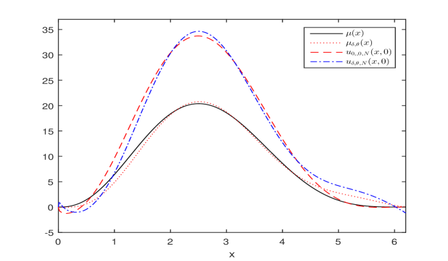
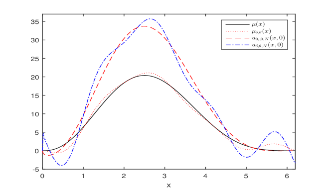
Figure 1: The profiles of the time averages $\mu(x)$ and $\mu_{\delta,\theta}(x)$, and traces of the corresponding solutions $u_{0,0,N}(x,0)$ and $u_{\delta,\theta,N}(x,0)$ defined by (22)-(23) with $q=0.0001$, $T=0.1$, $\delta=0.1$, $N=50$, $\theta=1$ (top) and $\theta=3$ (bottom).

Table 1: Dependence of the relative error $E_{\delta,N,\theta}$ on the input deviations.

	$\delta=0.0001$	$\delta=0.001$	$\delta=0.05$	$\delta=0.1$
$\theta=0.05$	0.00002	0.00023	0.0113	0.0226
$\theta=0.1$	0.00004	0.00044	0.0218	0.0436
$\theta=1$	0.00009	0.00087	0.0433	0.0866
$\theta=3$	0.00014	0.0014	0.0686	0.1372

An example for $\mu$ defined by (5) with applications to backward equations

By Theorem 1, $u(\cdot,0)$ can be restored from observation of $\mu=\mu_{\varepsilon}$ for an arbitrarily small $\varepsilon>0$, where $u$ is a solution of problem (1)-(2),(5). The following example illustrates a possibility to use this for the classical problem of restoration of $u(\cdot,0)$ from $u(\cdot,T)$. For this problem, $\mu=\mu_{\varepsilon}$ defined by (5) is actually unavailable for $\varepsilon>0$; instead, $u(\cdot,T)$ is available. Following the approach from Showalter (1985) and Clark and Oppenheimer (1994), we presume that the integral term in (5) is small, and we accept $u(\cdot,T)$ as an approximation of $\mu_{\varepsilon}$. This leads to acceptance of

$$u_{\varepsilon}(\cdot,0)\stackrel{{\scriptstyle{\scriptscriptstyle\Delta}}}{{=}}M_{\varepsilon,0}^{-1}u(\cdot,T)$$

as an approximation of $u(\cdot,0)$, where $M_{\varepsilon,0}$ is defined as $M_{0}$ with $\mu=\mu_{\varepsilon}$ defined by (5).

We did some numerical experiments to demonstrate potential applicability of this method. Figure 2 demonstrates the results for an example with $n=1$, $D=(0,L)$, and with the equation $u^{\prime}_{t}=u_{xx}^{\prime\prime}-qu$, where $q>0$, $L>0$. In these experiments, we first selected some profile $u(\cdot,0)$, then calculated $u(\cdot,T)$ using the corresponding Green’s function which is known for this toy forward equation; see e.g. [2], Chapter I.13. It can be noted that, for our experiment, it was sufficient to use for the Green’s function truncated sin series with 50 terms. Further, for this $u(\cdot,T)$, we calculated $u_{\varepsilon}(\cdot,0)\stackrel{{\scriptstyle{\scriptscriptstyle\Delta}}}{{=}}M_{\varepsilon,0}^{-1}u(\cdot,T)$ using equations (10)–(11). Finally, we compared $u_{\varepsilon}(\cdot,0)\stackrel{{\scriptstyle{\scriptscriptstyle\Delta}}}{{=}}M_{\varepsilon,0}^{-1}u(\cdot,T)$ with true $u(\cdot,0)$.

More precisely, we used truncated series

$$u_{\varepsilon,N}(x,0)=\sum_{k=1}^{N}\alpha_{k,\varepsilon}v_{k}(x),\quad N>0,$$ (25)

as an approximation of the solution, where $\alpha_{k,\varepsilon}$ are defined by (10)–(11) applied for $w=w_{\varepsilon}$.

The limit case where $\varepsilon=0$ was not excluded; in this case,

$$u_{0,N}(x,0)=\sum_{k=1}^{N}e^{\lambda_{k}T}g_{k}v_{k}(x)$$ (26)

is a solution based on straightforward truncation of the basis of eigenfunctions. Here $g_{k}\stackrel{{\scriptstyle{\scriptscriptstyle\Delta}}}{{=}}(u(\cdot,T),v_{k})_{H^{0}}$. For comparison purpose, we calculate this solution as well.

In addition, we calculated an estimate

$$\widetilde{u}_{\varepsilon,N}(x,0)=\sum_{k=1}^{N}\frac{1}{\varepsilon+e^{-\lambda_{k}T}}g_{k}v_{k}(x).$$ (27)

This estimate is implied by the quasi-boundary-value method that suggests to replace a ill-posed boundary condition $u(x,T)=f(x)$ by a well-posed condition $\varepsilon u(x,0)+u(x,T)=f(x)$ such as in Showalter (1985), Clark and Oppenheimer (1994).

Figure 2 shows the results for recovering $u(x,0)={\mathbb{I}}_{\{x>1.5\}}$ using our method with $\varepsilon=0.02$ and $N=18$. This figure shows $u_{\varepsilon,N}(x,0)$ (our method), $\widetilde{u}_{\varepsilon,N}(x,0)$ (quasi-boundary-value method), and $u_{0,N}(\cdot,0)$ (straightforward truncation (26)). Since $\varepsilon^{-1}\int_{0}^{\varepsilon}u(x,t)dt\approx u(x,0)$ in $L_{2}(D)$, it is natural to expect that the error for our solution and estimate (27) implied by the quasi-boundary-value method generate similar errors; Figure 2 shows that this holds for this example. In addition, it can be seen that these errors are less than the error for the estimate defined (26). It can be also noted that $u_{0,N}(x,0)$ defined by (26) blows up for $N\geq 19$. Since analysis of the backward parabolic equations is not in the focus of the present paper, we leave the future research the questions of selection of $N$ and $\varepsilon$, convergence analysis, and more precise comparison of different methods.

We used MATLAB and a standard PC; the calculation takes less than a second of CPU time for $N=1000$ in the setting of Figure 1, and for $N=100$ in the setting of Figure 2.

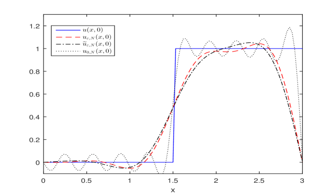
Figure 2: An initial profile $u(x,0)={\mathbb{I}}_{\{x>1.5\}}$ and its estimates calculated for $D=(0,3)$, $N=18$, $T=0.2$, and $\varepsilon=0.05$. Here $u_{\varepsilon,N}(x,0)$ is estimate (4), $\widetilde{u}_{\varepsilon,N}(x,0)$ is estimate (27), $u_{0,N}(x,0)$ is estimate (26).

We used MATLAB and a standard PC; the calculation takes less than a second of CPU time the calculation takes less than a second of CPU time for $N=100$ in the setting of Figure 2.

5 Conclusion

The paper study a possibility to recover a parabolic diffusion from its time-average for the case where the values at the initial time are unknown. This problem is reformulated as a new boundary value problem where a Cauchy condition is replaced by a condition involving the time-average of the solution. The paper establishes existence, uniqueness, and a regularity of the solution for this new problem and its modifications, including problems with singled out terminal values (Theorem 1). This Theorem 1 can be applied, for example, to the analysis of the evolution of temperature in a domain $D$, with a fixed temperature on the boundary. The process $u(x,t)$ can be interpreted as the temperature at a point $x\in D$ at time $t$. By Theorem 1, it is possible to recover the entire evolution of the temperature in the domain if one knows the average temperature over time interval $[0,T]$.

The suggested approach allows many modifications. An analog of Theorem 1 can be obtained for the setting where problem (1)–(3) is considered for a known pair $(u(\cdot,0),\mu)$ and for unknown $\varphi$ that has to be recovered. In this case, uniqueness of recovering $\varphi$ can be ensured via additional restrictions on its dependence on time; for example, it suffices to require that $\varphi(x,t)=\psi(t)v(x)$, where $\psi$ is a known function, and where $v\in H^{0}$ is unknown and has to be recovered.

It would be interesting to extend the result on the case where the operator $A$ is not necessarily symmetric and has coefficients depending on time. We leave this for the future research.

References

• [1] Beck, J.V. (1985). Inverse Heat Conduction. John Wiley and Sons, Inc..
• [2] Butkovskiy, A. G. (1982). Green’s Functions and Transfer Functions Handbook, Halstead Press - John Wiley & Sons, New York.
• [3] Clark G. W., Oppenheimer S. F. (1994) Quasireversibility methods for non-well posed problems, Electronic Journal of Differential Equations , no. 8, 1-9.
• [4] Dokuchaev, N.G. (2004). Estimates for distances between first exit times via parabolic equations in unbounded cylinders. Probability Theory and Related Fields, 129 (2), 290 - 314.
• [5] Dokuchaev, N. (2007). Parabolic equations with the second order Cauchy conditions on the boundary. Journal of Physics A: Mathematical and Theoretical. 40, pp. 12409–12413.
• [6] Dokuchaev N. (2008). Parabolic Ito equations with mixed in time conditions. Stochastic Analysis and Applications 26, Iss. 3, 562–576.
• [7] Dokuchaev, N. (2011). On prescribed change of profile for solutions of parabolic equations. Journal of Physics A: Mathematical and Theoretical 44 225204.
• [8] Dokuchaev, N. (2015). On forward and backward SPDEs with non-local boundary conditions. Discrete and Continuous Dynamical Systems Series A (DCDS-A) 35, No. 11, pp. 5335–5351
• [9] Glasko V. (1984). Inverse problems of mathematical physics. American Institute of Physics. New York.
• [10] Háo, D.N. (1998). Methods for inverse heat conduction problems. Frankfurt/Main, Bern, New York, Paris: Peter Lang Verlag.
• [11] Hao, D.N., Oanh, N.T.N. (2017). Determination of the initial condition in parabolic equations from integral observations. Inverse Problems in Science and Engineering 25 (8), 1138-1167.
• [12] Ladyzhenskaya, O. A. (1985). The boundary value problems of mathematical physics. Berlin etc., Springer-Verlag.
• [13] Ladyzhenskaja, O.A., Solonnikov, V.A., and Ural’ceva, N.N. (1968). Linear and quasi–linear equations of parabolic type. Providence, R.I.: American Mathematical Society.
• [14] Ladyzhenskaja, O.A., and Ural’ceva, N.N., Linear and quasilinear elliptic equations, Academic Press, New York, 1968.
• [15] Li J., Yamamoto M., Zou J. (2009). Conditional stability and numerical reconstruction of initial temperature. Commun. Pure Appl. Anal. 8, pp. 361?382.
• [16] Miller, K. (1973). Stabilized quasireversibility and other nearly best possible methods for non-well-posed problems. In: Symposium on Non-Well-Posed Problems and Logarithmic Convexity. Lecture Notes in Math. V. 316, Springer-Verlag, Berlin, pp. 161–176.
• [17] Miranker, W.L. (1961). A well posed problem for the backward heat equation. Proc. Amer. Math. Soc. 12 (2), pp. 243-274.
• [18] Prilepko A.I., Orlovsky D.G., Vasin I.A. (1984). Methods for Solving Inverse Problems in Mathematical Physics. Dekker, New York.
• [19] Seidman, T.I. (1996). Optimal filtering for the backward heat equation, SIAM J. Numer. Anal. 33, 162-170.
• [20] Showalter, R.E.. (1985). Cauchy problem for hyper-parabolic partial differential equations. In: Lakshmikantham, V. (ed.), Trends in the Theory and Practice of Non-Linear Analysis, Elsevier, North-Holland, pp. 421-425.
• [21] Tikhonov, A. N. and Arsenin, V. Y. (1977). Solutions of Ill-posed Problems. W. H. Winston, Washington, D. C.
• [22] Triet, L.M. and Phong, L.H. (2016). Regularization and error estimates for asymmetric backward nonhomogenous heat equation in a ball. Electronic Journal of Differential Equations, Vol. 2016, No. 256, pp. 1–12.
• [23] Triet, M. L.; Quan, P. H.; Trong ,D. D.; Tuan, N. H.. (2013). A backward parabolic equation with a time-dependent coefficient: Regularization and error estimates, J. Com. App. Math., No 237, pp. 432–441.
• [24] Tuan, N. H. and Trong, D. D. (2011). A simple regularization method for the ill-posed evolution equation. Czechoslovak mathematical journal 61 (1), pp. 85-95.
• [25] Tuan N. H. and Trong, D. D . (2014). On a backward parabolic problem with local Lipschitz source J. Math. Anal. Appl. 414 678?692.