High-Temperature Series Expansion for Spin-1/2 Heisenberg Models

Abstract

We present a high-temperature series expansion code for spin-1/2 Heisenberg models on arbitrary lattices. As an example we demonstrate how to use the application for an anisotropic triangular lattice with two independent couplings $J_{1}$ and $J_{2}$ and calculate the high-temperature series of the magnetic susceptibility and the static structure factor up to 12^th and 10^th order, respectively. We show how to extract effective coupling constants for the triangular Heisenberg model from experimental data on Cs₂CuBr₄.

ash]bashfontsize= pp]C++ son]C++ athematica]mathematica

PROGRAM SUMMARY

Program Title: LCSE
Authors: Andreas Hehn, Matthias Troyer
Licensing provisions: Use of the applications or any use of the source code requires citation of this paper.
Programming language: C++11, MPI for parallelization, Mathematica for analysis of results.
Computer: PC, cluster, or supercomputer
Operating system: Any, tested on Linux
RAM: 1 GB - 100 GB.
Number of processors used: 1 - 4096.
Keywords: linked cluster expansion, high-temperature series, series expansions, Heisenberg model.
Classification: 7.7
External routines/libraries: ALPS [1, 2, 3], GMP [4]
Nature of problem: Calculation of thermodynamic properties (magnetic susceptibility and static structure factor) for quantum magnets on arbitrary lattices. A particularly hard problem pose quantum magnets on so frustrated lattice geometries, as they can not be solved efficently by Quantum Monte Carlo methods.
Solution method: High-temperature series expansions employing a linked-cluster expansion allow to obtain a high-order series in the inverse temperature for thermodynamic quantities in the thermodynamic limit. The resulting high-temperature series are exact up to the expansion order. We implement the calculation of high-temperature series for the zero-field magnetic susceptibility and static magnetic structure factor for the spin-1/2 Heisenberg model on arbitrary infinite lattices in arbitrary dimension.
Program code and examples: http://www.comp-phys.org/lcse/

1 Introduction

Quantum antiferromagnets in low dimensions are a major topic in condensed matter physics. The initial reason for intensive study of antiferromagnetic systems was the discovery of antiferromagnetic order in the copper oxide layers of undoped parent compounds of high-temperature superconducting cuprates [5]. Since then, research on low dimensional antiferromagnetic structures has evolved into an independent field because these systems are strongly affected by quantum fluctuations and offer a great variety of exotic phases, like valence bond solids or quantum spin liquids [6]. From a theoretical perspective they are described by Heisenberg models, which are, due to their simplicity and the many exotic phases they exhibit, one of the most important class of toy models to study quantum phase transitions [7]. Furthermore, they can also serve a well controllable environment to investigate more general phenomena like Bose-Einstein condensation [8]. There exist plenty of experimental realizations for quantum magnets, such as the undoped La₂CuO₄, NaTiO₂ [9] or superconducting organic molecular crystals [10], to name a few. A common problem is the connection of the experiments to the theoretical models, i.e. the determination of coupling constants of theoretical models for a given material [11, 12].

An easy link between experiment and theory can be established by high-order high-temperature series expansions for the microscopic models. High-temperature series expansions have a long tradition in condensed matter physics [13, 14], and complement other numerical methods, such as exact diagonalization or quantum Monte Carlo, which are limited to small system sizes or non-frustrated systems, respectively. For translational invariant lattices, high-temperature series expansions provide results directly for the thermodynamic limit. The method is applicable to both simple bipartite spin models, as well as geometrically frustrated models or fermionic models [15] in arbitrary dimensions. The only approximation of the method is a finite order of the series.

In this paper we present a collection of applications to compute high-temperature series expansions for Heisenberg models on arbitrary lattices. As an example we compute the high-temperature series for an Heisenberg model on a triangular lattice with spatial anisotropy and show how to obtain estimates for the effective coupling constants for Cs₂CuBr₄. Previous studies of this model by Zheng et al. [16] derived the 10^th order series for the uniform magnetic susceptibility. We add two additional orders to this series and derived 10^th order series for the static magnetic structure factor.

2 Model

The spin-$1/2$ Heisenberg model is a lattice model where each site is occupied by a spin $i$ spanning a local Hilbert space $\mathcal{H}_{i}=\{|\uparrow\rangle,|\downarrow\rangle\}$. The spins couple along bonds of the lattice and are governed by the Hamiltonian

$$H=\sum_{\langle i,j\rangle}J_{i,j}\,\mathbf{S}_{i}\mathbf{S}_{j}\,,$$ (1)

where $\mathbf{S}_{i}$ are the spin-$1/2$ operators acting on the spin $i$, and $J_{i,j}$ are coupling constants for each bond $\langle i,j\rangle$ of the lattice. For the models considered, we only consider a small set of independent coupling constants $J_{i,j}\in\{J_{1},J_{2},\dots\}$. Bonds with the same coupling constant are said to be of the same type. While our application can handle up to four different bond types, we here focus on a model with only two bond types, namely the Heisenberg model on an anisotropic triangular lattice depicted in figure 1.

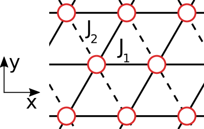
Figure 1: Triangular lattice with spatial anisotropy: exchange coupling $J_{1}$ along the solid lines and $J_{2}$ along the dashed lines.

With two freely tunable constants $J_{1},J_{2}$ the model covers three well known special cases: for $J_{1}=0$ the model decomposes into uncoupled spin chains, for $J_{2}=0$ the model is equivalent to the Heisenberg model on a square lattice, and for $J_{1}=J_{2}$ it becomes an isotropic triangular lattice.

The high-temperature series we obtain are symbolic polynomials in the variables $\beta J_{1}$, $\beta J_{2}$. As the coupling constants remain freely tunable our series is valid for both the ferromagnetic ($J_{1},J_{2}<0$) and the antiferromagnetic case ($J_{1},J_{2}>0$). In our analysis of the results we focus on the latter, as this case leads to geometric frustration on the triangular lattice as not all bonds can be satisfied classically. This enhances quantum fluctuations and promises an interesting phase diagram. Furthermore, the geometric frustration of the model makes it hard to study the system with the otherwise successful method of Quantum Monte Carlo (QMC) due to the sign-problem caused by the frustration. Hence the model renders an ideal playground for our high-temperature series expansions.

3 High-temperature Series Expansions

The high-temperature series expansions (HTE) of a thermodynamic quantity $Q$ in the inverse temperature $\beta$ can be written as

$$Q(\beta)=\sum_{n}a_{n}\beta^{n}\,.$$ (2)

For the Heisenberg model the quantities of interest are in many cases the partition function

$$Z=\operatorname*{Tr\,}_{\mathcal{H}}\mathrm{e}^{-\beta H}\approx\sum_{n=0}^{N}\frac{(-\beta)^{n}}{n!}\operatorname*{Tr\,}_{\mathcal{H}}H^{n}\,,$$ (3)

the uniform magnetic susceptibility

$$\chi=\beta^{-1}\frac{\partial^{2}}{\partial h^{2}}\ln Z\,,$$ (4)

and the spin-spin correlators

$$\langle S_{i}^{z}S_{j}^{z}\rangle=\frac{1}{Z}\operatorname*{Tr\,}_{\mathcal{H}}S_{i}^{z}S_{j}^{z}\mathrm{e}^{-\beta H}\,.$$ (5)

which are Fourier transformed to obtain the static structure factor

$$S(\mathbf{k})=\frac{1}{N}\sum_{i,j}\langle S_{i}^{z}S_{j}^{z}\rangle e^{-i\mathbf{k}(\mathbf{x}_{j}-\mathbf{x}_{i})}\,.$$ (6)

The trace in those equations runs over the full Hilbert space $\mathcal{H}=\mathcal{H}_{1}\otimes\mathcal{H}_{2}\otimes\dots$ of the quantum system. In the thermodynamic limit, this Hilbert space is of infinite dimension, as the lattice is infinite. However, for the series expanded term we may still obtain results in the thermodynamic limit. The limitations are a finite truncation order $N$ and a finite interaction range of $H^{n}$-terms, when $H$ is composed of local interactions.

To calculate the series we use the linked-cluster expansion, which expresses an extensive quantity $A$ on the lattice $L$ as a sum of so-called irreducible “weights” $w^{(g)}$, of small connected parts of the lattice, the embeddable connected graphs or clusters $g\in G_{L}$. As a graph $g$ can appear many times in the lattice the weight $w^{(g)}$ has to be multiplied by number of distinguishable embeddings in the lattice, the lattice constant $\mathrm{LC}(g)$

$$A=\sum_{g\in G_{L}}\mathrm{LC}(g)\cdot w^{(g)}\,.$$ (7)

For infinite, translational invariant lattices the quantity $A$ is usually expressed per site, in which case the embeddings are also counted per site.

The same idea applies to the graphs themselves. The extensive quantity $A^{(g)}$ defined on a graph $g$ is again expressed as a sum of contributions over all embeddable graphs $g^{\prime}$

$$A^{(g)}=\sum_{g^{\prime}\subset g}c(g^{\prime},g)\cdot w^{(g)}\,.$$ (8)

Similar to the lattice constant, $c(g^{\prime},g)$ denotes the number of ways that the graph $g^{\prime}$ can be embedded in the graph $g$. Note that this sum includes the graph $g$ itself. Starting from a graph $g_{1}$ of only a single vertex without any edges, where

$$A^{(g_{1})}=w^{(g_{1})}\,,$$ (9)

equation 8 defines a recursive scheme to determine the irreducible weight $w^{(g)}$ in the so-called subcluster-subtraction: given an extensive quantity $A^{(g)}$ of each graph $g$ we can obtain the irreducible weights $w^{(g)}$ by recursively subtracting the weights $w^{(g^{\prime})}$ of all graphs $g^{\prime}$ embeddable in $g$. The weights $w^{(g)}$ may then be combined to $A$ defined on the full lattice in equation (7).

For an infinite lattice the number of contributing graphs $g$ is evidently infinite. However, due to the finite range of the $H^{n}$-terms in a high-temperature series expansion all irreducible weights $w^{(g)}$ for graphs with more than $n$ edges hosting a pair-wise interaction, such as the $\mathbf{S}_{i}\mathbf{S}_{j}$ interaction of the Heisenberg model, vanish. Hence, for a finite expansion order $N$ we only need to consider a small fraction of all embeddable graphs $G_{L}$, namely all embeddable graphs with $n\leq N$ edges.

Putting the pieces together, the computation of an high-temperature series consists of four stages:

1. finding all contributing connected graphs

2. computing the extensive quantity $A^{(g)}$ for each graph

3. performing a subcluster-subtraction to obtain irreducible weights $w^{(g)}$

4. embedding the graphs in the lattice and summing up the weights accordingly.

4 Running the Application

Similar to those four stages running our code for the spin-1/2 Heisenberg model on a given lattice involves three steps, each carried out by a dedicated application as shown in the respective example calls:

1. the graph generation, creating a list of all graphs embeddable into the desired lattice graph_generator latticeparam.json graphlist.graphs

2. the weight computation, calculating the contribution to the free energy series, magnetic susceptibility series and spin structure factor series for each graph spin1_2_heisenberg_hte_compute_weights_2_variables 10 graphlist.graphs raw_heisenberg.series

3. and finally the embedding step, performing the subcluster-subtraction and embedding into the lattice. spin1_2_heisenberg_hte_reduce_embed_weights latticeparam.json graphlist.graphs raw_heisenberg.series reduced_heisenberg_series

In the following sections we explain these steps and the associated applications in more detail.

4.1 Graph Generation

The first program graph_generator ¡parameterfile¿ ¡outputfile¿ generates all embeddable graphs with up to $N$ edges for a lattice specified using the ALPS lattice library [1, 2]. Starting from a single vertex it generates graphs by recursively adding edges, checking for already seen isomorphic graphs using a variant of the McKay algorithm [17, 18] and trying to embed these graphs in the lattice. The program takes two arguments:

• ¡parameterfile¿, the name of a parameter file in JSON format, and

• ¡outputfile¿, the name of the output file in which the found graphs are stored.

Listing 2 shows the parameter file used for the anisotropic triangular lattice.

”lattice”: ”lattice_library” : ”custom_lattices.xml”, ”type”: ”anisotropic triangular lattice 2 couplings”, ”L”: 40, , ”num_edges”: 12, ”homogeneous_model” : true

Figure 2: The parameter file for the graph_generator program used in our example.

The first parameter, ”lattice”, describes the lattice for which the embeddable graphs are generated. The lattices are provided by the ALPS lattice library which offers a big selection of predefined lattice and is easily extensible.

The parameters ”type” and ”L” are the name and the extent of the lattice and are passed through to the ALPS lattice library. As our example relies on a lattice which is not part of the standard ALPS lattice library, a custom library file is loaded via the ”lattice_library” parameter. Note that ”L” is not the size of the (infinite) lattice used in the calculations, but indicates a finite lattice large enough so that embedded clusters starting at the center do not extend to the boundary.

The next parameter, ”num_edges”, sets the upper limit on the number of edges of the generated graphs and should match the desired order of the series to be computed.

The last parameter tells the graph generator that all terms of the Hamiltonian, regardless of the edge type, are of the same form ($\mathbf{S}_{i}\mathbf{S}_{j}$).

For the anisotropic triangular lattice depicted in figure 1 we found $4^{\prime}821^{\prime}837$ embeddable graphs with $n\leq 12$ edges.

4.2 Weight Computation

The weight computation is the most expensive part of the procedure. Due to the rapidly growing number of graphs for higher orders, as well as the exponentially growing Hilbert space with the number of sites in a graph, the computational effort grows exponentially with the desired order of the series. We provide applications for up to four independent coupling constants spin1_2_heisenberg_hte_compute_weights_1_variables spin1_2_heisenberg_hte_compute_weights_2_variables spin1_2_heisenberg_hte_compute_weights_3_variables spin1_2_heisenberg_hte_compute_weights_4_variables Each application accepts the following three parameters … [–suscept-only] ¡order¿ ¡graphfile¿ ¡outputfile¿ where the first mandatory parameter ¡order¿ is the desired order of the expansion, followed by ¡graphfile¿, the name of the file containing the list of graphs for which the weights should be computed, and ¡outputfile¿, the name of the output file. For each graph the application will compute the series for the partition function, the susceptibility and the equal-time $S^{z}_{i}S^{z}_{j}$ correlator for the static structure factor $S(\mathbf{k})$. All results will be appended to the combined output file. If the structure factor is not of interest, the mandatory arguments can be preceded by the optional switch –suscept-only, telling the application to omit the calculation of the correlator series. This allows to focus on pushing the susceptibility to the highest possible order.

If the output file ¡combinedseriesdb¿ already exists, the program will only compute and append the weights of the missing graphs. Therefore the computations can be interrupted at any time and may be continued by re-executing the same command.

For short series the regular applications for desktop computers suffice. However, two to three additional orders may be achieved running the MPI-parallelized versions of the applications on a cluster or supercomputer. The MPI applications will group the graph contributions to be computed in tasks of a few graphs each and schedule those tasks across all available MPI processes. The applications, which have to be executed within an MPI environment, share the same command line arguments as their non-MPI counterparts, but take three additional optional parameters controlling the parallelization: … [–suscept-only] ¡order¿ ¡graphfile¿ ¡outputfile¿ [threadspp] [checkp_interval] [task_size]

• threadspp is the number of threads per MPI process (default: 16). In most cases a single MPI process per cluster node should be used, running one thread per CPU-core of the node.

• checkp_interval sets the interval of checkpoints in seconds (default: 30). At the end of each interval the completed computation tasks will be collected from all MPI processes and stored in the output database.

• task_size controls the size of a computation task, i.e. the number of graphs per computation task (default: 15). Note that the program will only save completed tasks, where all graph contributions have been calculated, to the database at the checkpoints. Large task_size and checkp_interval values may therefore result in dropping many computed contributions in incomplete tasks at termination of the program. Very small values, on the other hand, may cause considerable network traffic on the cluster.

If these optional arguments are not specified their default value will be used.

4.3 Subcluster-Subtraction and Embedding

Once the raw weights are calculated for all contributing graphs, the spin1_2_heisenberg_hte_reduce_embed_weights ¡parameterfile¿ ¡graphfile¿ ¡combinedseriesdb¿ ¡seriesdb_prefix¿ program will perform the subcluster-subtraction and sum up the irreducible weights according to the embeddings of the graphs in the the lattice. For this task the program requires four arguments:

• ¡parameterfile¿, the name of the json file containing the lattice parameters,

• ¡graphfile¿ the name of the file containing the list of contributing graphs for the lattice,

• ¡combinedseriesdb¿, the name of the file with the combined raw weights for the partition function, the susceptibility and optionally the two-site correlator for all contributing graphs from the previous step, and

• ¡seriesdb_prefix¿, a prefix for the intermediate files the program will generate.

From the combined raw weights file the program generates three files containing the full graph contributions before the subcluster-subtraction:
¡sp¿_raw_mBetaF.series free energy ($-\beta F$) ¡sp¿_raw_suscept.series susceptibility ¡sp¿_raw_SzSz_correlator.series $S^{z}_{i}S^{z}_{j}$ correlator
and three files with the irreducible weights after the subcluster-subtraction:
¡sp¿_red_mBetaF.series free energy ($-\beta F$) ¡sp¿_red_suscept.series susceptibility ¡sp¿_red_SzSz_correlator.series $S^{z}_{i}S^{z}_{j}$ correlator.
The prefix ¡sp¿ of the filenames is substituted by the value of the command line argument ¡seriesdb_prefix¿ mentioned above.

Once more, if the output file already exists any already calculated quantity will be taken into account and only missing weights will be appended. As the weights of the graphs are independent of the underlying lattice, the weight files may contain weights for graphs not contributing to the lattice. Once the subcluster-subtraction is completed and all irreducible weights are available, the program tries to embed all graphs from the graph list file into the lattice. When the embedding is completed it will print out the resulting series in Mathematica compatible format to standard-out.

5 Series Analysis

Analysis of the high-$T$ series is done in Mathematica, which allows us to easily perform symbolic manipulations and has many of the needed tools, most notably Padé approximants, built-in. Along with the high-temperature series expansion application code we ship two Mathematica packages which complement the built-in tools and provide functions to simplify common tasks of the analysis. Here we show how to extract estimates for the coupling constants for the Heisenberg model from susceptibility measurements on Cs₂CuBr₄, using Padé approximants constructed from the high-temperature series.

5.1 Padé Approximants

In most cases the bare series have a very limited convergence radius, which is hard to estimate if only few coefficients are available. A common method to extend the convergence radius of such a power series and to provide a rough error estimate are Padé approximants [19]. Padé approximants are a simple analytical continuation of the power series, which, in contrast to the bare series, can represent simple poles in the complex plane and therefore may better approximate the original function. A Padé approximant to a function $f(x)$ is a rational function

$$P[L,M](x)=\frac{a_{0}+a_{1}x+\dots+a_{L}x^{L}}{1+b_{1}x+\dots+b_{M}x^{M}}$$ (10)

of numerator degree $L$ and denominator degree $M$, whose power series is identical to the power series of the function $f(x)$ up to the order $L+M$. The individual coefficients $a_{i}$, $b_{j}$ are uniquely defined by this condition. Error estimates from Padé approximants have to be interpreted with care as various approaches exist and none of them provides rigorous error bars [20, 21]. A simple, yet effective method is to inspect the behavior and spread of the Padé approximants $P[L,N-L](x)$ for all $0\leq L\leq N$ with increasing order $N$. Approximants are trusted as long as most approximants of a given order $N$ agree well. Higher confidence is usually put on balanced approximants, where the numerator and denominator are of roughly same degree.

Special attention has to be payed to the pole structure of the approximant. Approximants $P[L,M]$ exhibiting a close root-pole pair in the complex plane are considered defective, since the pair would virtually cancel and add no further information compared to a Padé approximant of lower order.

5.2 Extraction of Coupling Constants

The effective coupling constants of the Heisenberg model for a real quantum magnet can be estimated by fitting the Padé approximants of the magnetic susceptibility $\chi(T)$ to experimental data. As an example we illustrate how to determine the coupling constants of the Heisenberg model on an anisotropic triangular lattice for Cs₂CuBr₄. The full procedure can be found in the Mathematica notebook in the example folder of the code package.

In the beginning of the notebook we load the Mathematica packages shipped with the code and paste the high-temperature series $\chi/\beta$ copied from the output of the series expansion application ¡¡ ”padeanalysis.m” ¡¡ ”paderesidualanalysis.m” chiOverBeta = 1/4 - 1/8*K + (*…*) - 1/4*B + (*…*) where the the symbolic variables B and K correspond to $\beta J_{1}$ and $\beta J_{2}$, respectively.

For the fit to experimental data, three free parameters of the susceptibility function $\chi(T)$ of our model need to be determined: the Heisenberg couplings $J_{1}$, $J_{2}$ and the $g$-factor. As the couplings $J_{1}$ and $J_{2}$ appear as non-linear parameters in the Padé approximants, we determine these parameters by a parameter scan on an equidistant grid, calculating the sum of squared residuals to the experimental data for each grid point.

The range for the grid is derived from the behavior of the system at very high temperatures, where the Curie-Weiss law

$$\chi(T)=\frac{C}{T_{CW}+T}$$ (11)

applies. Here $\chi(T)$ is the magnetic susceptibility per mole, $C$ is the Curie constant $C=N_{A}g^{2}\mu_{0}\mu_{b}^{2}/4k_{B}$ and $T_{CW}$ is the Curie-Weiss temperature. From a fit to the experimental data we obtain a first estimate for the $g$-factor and the Curie-Weiss temperature which relates to the coupling constants of our system through mean-field theory

$$T_{CW}=J_{1}+J_{2}/2\,.$$ (12)

Depending on the temperature range considered, the fit of the Curie-Weiss law for Cs₂CuBr₄ yields $1.94<g<2.03$ and $3\mathrm{K}<T_{CW}<20\mathrm{K}$ (not shown). To benefit from this first estimate the free parameter $J_{2}$ in our analysis is substituted by $T_{CW}$ according to eq. 12.

For the parameter scan we define an equidistant grid for $5\mathrm{K}\leq T_{CW}\leq 20\mathrm{K}$ and $0.1\mathrm{K}\leq J_{1}\leq 15\mathrm{K}$ with a grid spacing of $0.1\mathrm{K}$ for each parameter. The Mathematica packages, loaded before, offer a set of tools for this scan, which are controlled by a common parameter set. Such a parameter set is created with the CreatePadeResidualLandscapesParameterSet function from a list of Padé parameters $[L,M]$ and the ranges forming the two-dimensional grid: TcwRange = Range[5, 20, 1/10]; JRange = Range[1/10, 150/10, 1/10]; PadeParameters = AllPadeParametersOfOrder[12]; parameterset = CreatePadeResidualLandscapesParameterSet[ PadeParameters, TcwRange, JRange ];

As Padé approximants are univariate, the tools require a function to reduce the multivariate high-temperature series to a univariate series for the parameters of a grid point. seriesforparameters = Function[ tcw, J1, Evaluate[Simplify[ chiOverBeta /. K -¿ ((2*tcw/J1 - 2)*B) ] ] ]; The defined function seriesforparameters takes the two parameters of a grid point $T_{CW}$, $J_{1}$ and returns a univariate series in B $=\beta J_{1}$, where all occurrences of K were substituted by K $=J_{2}/J_{1}\cdot$B. Internally the tools use this function to generate Padé approximants $P[L,M]($B$)$ for fixed $T_{CW}$.

To derive a function for the susceptibility $\chi(T)$ with the physical units from a Padé approximant another (higher-order) function has to be defined. This function takes the approximant $P[L,M]($B$)$, the parameters of the grid point $T_{CW}$ and $J_{1}$, as well as the experimental data and returns a function $\chi(T)$, where the temperature $T$ remains the only undetermined variable. modelfromapproximant = Function[ approximant, tcw, J1, data, Function[ T, Evaluate[ With[ fkt = g2*A*4*1/T*Simplify[ approximant /. B -¿ J1/T ] , fkt /. FindFit[data, fkt, g2, T] ] ] ] ]; In our example the function modelfromapproximant creates $\chi(T)$ from an approximant by substituting B for fixed $J_{1}$, multiplying by the constant $4$A $=4C/g^{2}$ and $1/T$, and fitting the remaining linear $g^{2}$ factor to the experimental data using Mathematica’s FindFit function.

Finally we construct Padé approximants and a corresponding model function $\chi(T)$ for each grid point $T_{CW},J_{1}$ of the parameter scan and compute for each function the sum of the squared residuals

$$R=\sum_{i}(\bar{\chi}_{i}-\chi(T_{i}))^{2}$$ (13)

against the experimental data points $(T_{i},\bar{\chi}_{i})$. We named the sums of squared residuals on the grid for a fixed Padé parameter pair $[L,M]$ a residual landscape. For the involved task of computing those residual landscapes for multiple Padé parameter pairs, the supplied Mathematica package offers a convenient function ComputeResidualLandscapes[seriesForParametersF, symbol, filterPredicates, modelFromPadeApproximantF, data, parameterset] The most important parameter is the parameterset we encountered before, which defines the grid and contains the list of Padé parameters $[L,M]$ for which the residual landscapes are calculated. The function returns a list, with an residual landscape — a two-dimensional array containing the sums of squared residuals for each grid point — for each Padé parameter pair $[L,M]$ of the parameter set. The seriesForParametersF parameter is the user defined function to generate a univariate series for a grid point and symbol is the symbol of the variable of this series. These arguments will be used to build Padé approximants. The filterPredicates parameter takes a list of predicates which are applied to the resulting approximants. Approximants not fulfilling the predicates are immediately dropped.
The next parameter, modelFromPadeApproximantF, defines how to build a model function $\chi(T)$ from the approximant. It expects a function taking four arguments, the approximant, the two parameters of a grid point, and the data for the fit. The last parameter data is the set of experimental data points.

For the example the function is called as follows residuals12thorder = ComputeResidualLandscapes[ seriesforparameters, B, HasNoCloseRootPolePair[0.1], modelfromapproximant, experimentaldata, parameterset ]; where HasNoCloseRootPolePair[0.1] is a predicate to filter all defective Padé approximants, i.e. approximants a root-pole pair in the complex plane with a distance less than $0.1$.

Once the computation is completed, residuals12thorder contains twelve residual landscapes for the Padé parameters $[L,12-L]$, $0\leq L\leq 12$. From this list of landscapes the best fitting Padé of each grid point can be selected by minimalresiduals = SelectMinima[residuals12thorder, parameterset ]; returning a list with two elements, where the first element is the minimum sums of squared residual for each grid point, and the second element is a two-dimensional array of Padé parameter pairs $[L,M]$ exhibiting the minimum of the corresponding point.

6 Experiments on Cs₂CuBr₄

The Cs₂CuBr₄ crystals with an orthorhombic (Pnma) structure were grown from aqueous solution with the evaporation method. This implies that with respect to salts CsBr and CuBr₂ the 2:1 stoichiometric mixture was used for the growth. For the crystal growth process a small evaporation rate such as $25\mathrm{mg}/\mathrm{h}$ was used to reach an appropriate crystallization rate. This leads to a very good crystal quality. The sample was crystallized within 4 weeks at room temperature [22]. The magnetic susceptibility measurement of the Cs₂CuBr₄ single crystal was determined in the temperature range between $2\mathrm{K}\leq T\leq 300\mathrm{K}$ and in a magnetic field $B=1\mathrm{T}$ using a Quantum Design SQUID magnetometer. The measurement was performed on a single crystal, which was oriented parallel to the crystallographic $b$ axis. The temperature-independent diamagnetic core contribution has corrected the magnetic contribution of the sample holder and the constituents according to [23]. The determination of the magnetic background is important, especially at high temperatures, where the magnetic signal of this compound is small.

7 Results

For the Heisenberg model on the anisotropic triangular lattice depicted in figure 1, we obtained the high-temperature series for the magnetic susceptibility up to 12^th order and the series for the static spin structure factor up to 10^th order. The coefficients of the plain high-temperature series can be found in table 1 and the example folder of the program sources, respectively. In the following we compare the computed series to results from Quantum Monte Carlo simulations on the same lattice for the case of an antiferromagnetic square sub-lattice with ferromagnetic couplings along the diagonal chains $J_{1}>0,J_{2}<0$ and we compare the fully antiferromagnetic case $J_{1}>0,J_{2}>0$ with experimental results on Cs₂CuBr₄.

7.1 Comparison to Quantum Monte Carlo

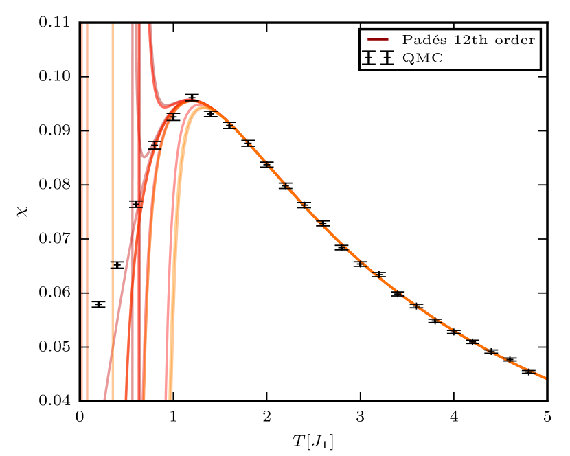
Figure 3: Comparison of Padé approximants to the $12\textsuperscript{th}$ order series of the magnetic susceptibility $\chi(T)$ for a non-frustrated system with ferromagnetic chain couplings ($J_{1}=1,J_{2}=-1$) with Quantum Monte Carlo simulations.

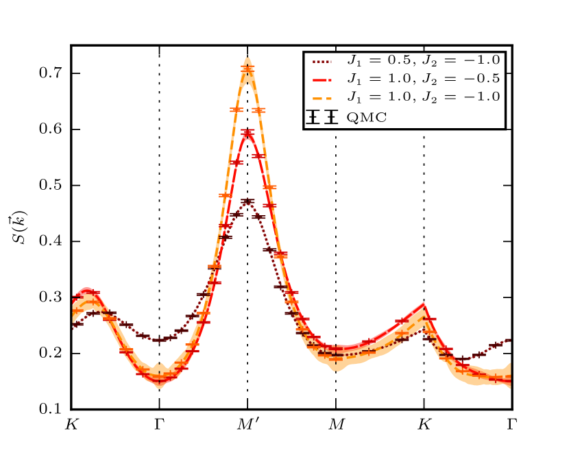
Figure 4: Comparison of the static structure factor $S(\mathbf{k})$ computed by series expansions (lines) against Quantum Monte Carlo simulations (points with error-bars) for a non-frustrated systems with ferromagnetic chain couplings $J_{1}>0,J_{2}<0$ at $T=1.8\,J_{1}$. The path through the Brillouin zone is shown in figure 7. While discrete error-bars represent the standard deviation of Monte Carlo samples, the continuous error-areas around the lines represent the spread of Padé approximants and are not rigorous error estimates.

In contrast to the fully antiferromagnetic case, the mixed case with ferromagnetic couplings along the chains $J_{1}>0,J_{2}<0$ is not frustrated and can be treated efficiently with Quantum Monte Carlo methods as it is not subject to the well-known sign-problem. We performed Quantum Monte Carlo simulations for three exemplary cases $J_{1}/J_{2}=\{1/2,1,2\}$ using the dirloop_sse application of ALPS[1, 2, 3], which is based on the stochastic series expansion (SSE) method. Each data point is computed from $5\cdot 10^{4}$ samples on a lattice patch of $64^{2}$ sites. Figure 3 shows the temperature behavior of the magnetic susceptibility for $J_{1}/J_{2}=1$ obtained from Quantum Monte Carlo together with the non-defective Padé approximants $P[L,M]$ with $11\leq L+M\leq 12$ continuing the calculated 12^th order series. Above $T\approx 1.2J_{1}$ the spread of the Padé approximants is negligible and the approximants are in excellent agreement with the Monte Carlo results. Below $T\approx J_{1}$ the different Padé approximants start to spread drastically. Even in this temperature regime, down to $T\approx 0.6J_{1}$, a few approximants agree well with Monte Carlo. In this regime, however, a prediction solely based on the computed series would be hard to justify, due to the broad spread of the different approximants. For the other parameters $J_{1}/J_{2}=\{1/2,2\}$, a very similar spreading behavior and agreement with Quantum Monte Carlo data of the Padé approximants is observed (not shown).

Also for the spin structure factor $S(\mathbf{k})$ (fig. 4), the 10^th order series and Quantum Monte Carlo estimates agree beautifully down to $T\approx 1.8J_{1}$ or rather $T\approx 1.4J_{1}$, depending on the particular couplings. For lower temperatures the predictions from the series data become increasingly unreliable as the Padé approximants start spreading. Both methods consistently display the peak at $M^{\prime}$, which is a residue of antiferromagnetic ordering at $T=0$.

7.2 Comparison with Cs₂CuBr₄

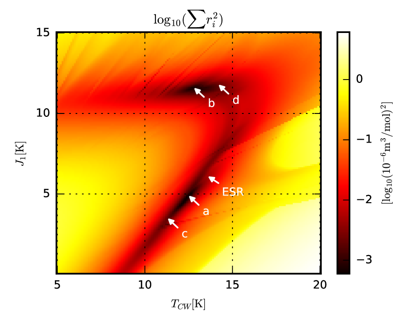
Figure 5: Sum of squared residuals $r^{2}$ of the best fitting Padé approximants $P[L,M]$ for the computed magnetic susceptibility $\chi(T)$ compared to data for CS₂CuBr₄ with $T>7K$. Minima: (a) $T_{CW}=12.5\mathrm{K}$, $J_{1}=4.9\mathrm{K}$, (b) $T_{CW}=12.8\mathrm{K}$, $J_{1}=11.6\mathrm{K}$; for comparison in figure 6: (c) $T_{CW}=11.3\mathrm{K}$, $J_{1}=3.5\mathrm{K}$, (d) $T_{CW}=14.2\mathrm{K}$, $J_{1}=11.8\mathrm{K}$; (ESR) values obtained from ESR study $T_{CW}=13.6\mathrm{K}$, $J_{1}=6.1\mathrm{K}$ [12].

For Cs₂CuBr₄ we fitted the 12^th order series to the experimental data on the magnetic susceptibility. The model functions $\chi(T)$ with proper units are obtained from the bare series as described in the previous section. Figure 5 shows the sum of squared residuals compared to the experimental data of the best fitting non-defective Padé approximants $P[L,M]$ with $9\leq L+M\leq 12$ for each point of the grid. Note that we only consider $T>7K$ for the procedure, as the approximants will not approximate the underlying function well for low temperatures. The cutoff temperature was chosen slightly below the point the different approximants start to spread significantly. Higher order calculations might reduce this spreading temperature further, however, we do not expect significant changes with 1-2 additional orders, as we see only marginal improvement from 10^th to 12^th order.

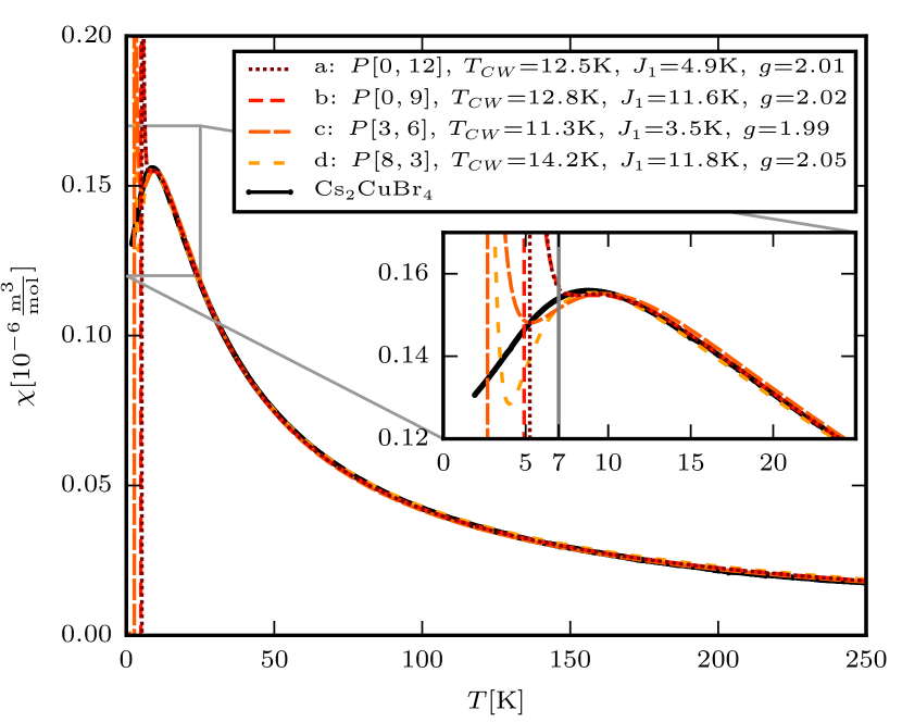
Figure 6: Padé approximants fitted to Cs₂CuBr₄ data for $T>7K$.

The parameter scan reveals two shallow elliptical valleys of the residuals centered around the local minima at $T_{CW}=12.5\mathrm{K}$, $J_{1}=4.9\mathrm{K}$ and $T_{CW}=12.8\mathrm{K}$, $J_{1}=11.6\mathrm{K}$, respectively. For both points the corresponding Padés behave remarkably similar. Both Padés yield an excellent fit to the experimental data within the considered temperature range (fig. 6). Also both Padés slightly overestimate the susceptibility for high-temperatures and slightly underestimate close to the maximum, before both Padés diverge around $T=6\mathrm{K}$.

However, also parameters at the verge of the valleys of the residual landscape, e.g. at $T_{CW}=11.3\mathrm{K}$, $J_{1}=3.5\mathrm{K}$ and $T_{CW}=14.2\mathrm{K}$, $J_{1}=11.8\mathrm{K}$ ( (c) and (d) in figures 5 and 6), fit the data very well and illustrate how a wide range of parameters along the valleys leads to comparable fits. The extracted $g$-factors of all presented approximants all lie within the range expected from the Curie-Weiss law, but underestimate the $g$-factor obtained from spin resonance experiments $g=2.09$ [12].

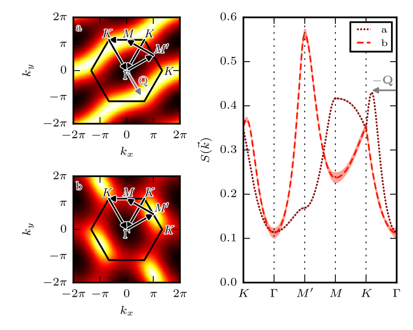
Figure 7: Static structure factor $S(\mathbf{k})$ for (a) $T_{CW}=12.5\mathrm{K}$, $J_{1}=4.9\mathrm{K}$ and (b) $T_{CW}=12.8\mathrm{K}$, $J_{1}=11.6\mathrm{K}$ at $T=15\mathrm{K}$. Error bars represent the spread of Padé approximants and are not rigorous error estimates. For (a) $S(\mathbf{k})$ exhibits a peak at $\mathbf{Q}=0.54\mathbf{b}_{J_{2}}$ hinting at incommensurate ordering.

Physically the valleys correspond to two different regimes. In case (a) the triangular model is dominated by the antiferromagnetic chain couplings $J_{2}=15.2\mathrm{K}$ competing with a significantly smaller square lattice coupling of only $J_{1}=4.9\mathrm{K}$ ($J_{1}/J_{2}=0.3(2)$). This is also reflected in static structure factor $S(\mathbf{k})$ shown in figure 7, which features a plane wave structure along the axis of the chain couplings, with maxima close to the antiferromagnetic ordering vector of decoupled chains. The plane wave is only slightly wiggled by the competing square lattice couplings, pushing the maxima further to the corners of the Brillouin zone to $\mathbf{Q}=0.54\mathbf{b}_{J_{2}}$, where $\mathbf{b}_{J_{2}}$ is the reciprocal vector corresponding to the lattice vector $\mathbf{a}_{J_{2}}$ along the $J_{2}$ bonds. The other valley (b) corresponds to a triangular lattice with a strong square lattice coupling $J_{1}=11.6\mathrm{K}$ perturbed by only a very small chain coupling $J_{2}=2.4\mathrm{K}$ ($J_{2}/J_{1}=0.2(1)$). Here the structure factor exhibits a peak at the symmetry point $M^{\prime}$ as one would expect from an antiferromagnetic ordering on the square lattice.

Previous studies of Cs₂CuBr₄ using high-temperature series expansions by Zheng et al. [16] obtained $J_{1}=6.99\mathrm{K}$ and $J_{2}=14\mathrm{K}$ ($T_{CW}=14\mathrm{K}$, $J_{1}/J_{2}=0.5$) from the 10^th order series of the susceptibility, but also report that a wide range of ratios $0.35<J_{1}/J_{2}<0.55$ give comparable fits. Those values reside at the upper end of our residual valley (a). Another study extracted the Heisenberg couplings from high-field electron-spin-resonance measurements with harmonic spin-wave theory [12]. Their findings of $J_{1}=6.1(3)\mathrm{K}$ and $J_{2}=14.9(7)\mathrm{K}$ corresponds to a Curie-Weiss temperature of $T_{CW}=13.6(2)\mathrm{K}$ and $J_{1}/J_{2}=0.41(0)$. While also their coupling ratio seems significantly higher than the $J_{1}/J_{2}=0.3(2)$ obtained here, the parameters lie well within valley (a) (fig. 5) and are plausible candidates.

Further evidence for case (a) are neutron-scattering experiments on Cs₂CuBr₄ [24, 25], which revealed an incommensurate ordering vector of $\mathbf{Q}=0.575\mathbf{b}_{J_{2}}$ at zero magnetic field, consistent with our predictions from the high-temperature series for point (a) (fig. 7). While the predicted ordering vector for fit (a) $\mathbf{Q}=0.54\mathbf{b}_{J_{2}}$ is slightly smaller than the ordering vector measured by neutron-scattering, one has to bear in mind that they were obtained at significantly different temperatures of $T=15\mathrm{K}$ and $T=60\mathrm{mK}$, respectively, and might further converge. Zheng et al. [16] and Ono et al. [25] also estimate the coupling ratio $J_{1}/J_{2}$ from the ordering vector by comparison with various theoretical models: for the ground-state of the classical spin model on an anisotropic triangular lattice, where neighboring spins on the square sub-lattice are rotated by the angle $q$, the incommensurate ordering vector yields the ratio $J_{1}/J_{2}=-2\cos(q)=-2\cos(\mathbf{Q}\cdot\mathbf{a}_{J_{2}}/2)=0.47$. Their comparison with theories including the quantum fluctuations, which are enhanced by the geometric frustration of the model, suggest even higher values, namely $J_{1}/J_{2}\approx 0.56$ for large-$N$ Sp($N$) theory [26], and $J_{1}/J_{2}\approx 0.72$ for zero-temperature series expansions [27]. While the high correction compared to the classical value found in zero-temperature series expansions is questioned by the authors in their later study [16], the real coupling ratio seems to be above the ratio $J_{1}/J_{2}=0.3(2)$ for the optimal fit we found for valley (a) and closer to the ESR value in figure 5.

8 Extensibility

The presented applications for Heisenberg models are built with a modular C++ framework for high-temperature series expansions we developed. The framework provides generic algorithms for the graph generation, the high temperature expansion and the graph embeddings. With little effort the presented application could be generalized to include Dzyaloshinskii-Moriya terms or new applications for fermionic lattice models, such as the $t$-$J$ can be written based on the existing implementation of the algorithms.

9 Conclusion

We presented a set of applications and Mathematica packages to compute and analyze high-temperature series for the free energy, the uniform magnetic susceptibility and the static structure factor of Heisenberg models on arbitrary lattices with up to four independent coupling constants. As an example we computed the high-temperature series for the anisotropic triangular lattice and showed how to obtain estimates for the coupling constants by fitting the Padé approximants to susceptibility data for Cs₂CuBr₄.

While the obtained high-temperature series for the anisotropic triangular lattice can be directly applied to other realizations of the same model, such as Cs₂CuCl${}_{4}~{}$[28] or various organic superconducting materials [29, 16], the computer programs allow easy access to high-temperature series of all quantum magnets, in arbitrary dimensions, which can be described by spin-$1/2$ Heisenberg models on regular lattices, including layered quasi two-dimensional lattices or dimerized systems. Therefore the presented applications may prove to be a powerful tool in the lab, to gain a better understanding experimental results.

References

- [1] A. Albuquerque, F. Alet, P. Corboz, P. Dayal, A. Feiguin, S. Fuchs, L. Gamper, E. Gull, S. Gürtler, A. Honecker, R. Igarashi, M. Körner, A. Kozhevnikov, A. Läuchli, S. Manmana, M. Matsumoto, I. McCulloch, F. Michel, R. Noack, G. Pawłowski, L. Pollet, T. Pruschke, U. Schollwöck, S. Todo, S. Trebst, M. Troyer, P. Werner, S. Wessel, The ALPS project release 1.3: Open-source software for strongly correlated systems, Journal of Magnetism and Magnetic Materials 310 (2, Part 2) (2007) 1187 – 1193, proceedings of the 17th International Conference on MagnetismThe International Conference on Magnetism. doi:10.1016/j.jmmm.2006.10.304.
- [2] B. Bauer, L. D. Carr, H. G. Evertz, A. Feiguin, J. Freire, S. Fuchs, L. Gamper, J. Gukelberger, E. Gull, S. Guertler, A. Hehn, R. Igarashi, S. V. Isakov, D. Koop, P. N. Ma, P. Mates, H. Matsuo, O. Parcollet, G. Pawłowski, J. D. Picon, L. Pollet, E. Santos, V. W. Scarola, U. Schollwöck, C. Silva, B. Surer, S. Todo, S. Trebst, M. Troyer, M. L. Wall, P. Werner, S. Wessel, The ALPS project release 2.0: open source software for strongly correlated systems, Journal of Statistical Mechanics: Theory and Experiment 2011 (05) (2011) P05001. doi:10.1088/1742-5468/2011/05/P05001.
- [3] http://alps.comp-phys.org.
- [4] http://www.gmplib.org.
- [5] D. Vaknin, S. K. Sinha, D. E. Moncton, D. C. Johnston, J. M. Newsam, C. R. Safinya, H. E. King, Antiferromagnetism in , Phys. Rev. Lett. 58 (26) (1987) 2802–2805. doi:10.1103/PhysRevLett.58.2802.
- [6] K. Matan, T. Ono, Y. Fukumoto, T. J. Sato, J. Yamaura, M. Yano, K. Morita, H. Tanaka, Pinwheel valence-bond solid and triplet excitations in the two-dimensional deformed kagome lattice, Nat. Phys. 6 (2010) 865–869. doi:10.1038/nphys1761.
- [7] S. Sachdev, Quantum Phase Transitions, Cambridge University Press, 1999.
- [8] T. Giamarchi, C. Ruegg, O. Tchernyshyov, Bose-einstein condensation in magnetic insulators, Nature Physics 4 (2008) 198–204. doi:10.1038/nphys893.
- [9] S. J. Clarke, A. J. Fowkes, A. Harrison, R. M. Ibberson, M. J. Rosseinsky, Synthesis, Structure, and Magnetic Properties of NaTiO2, Chemistry of Materials 10 (1) (1998) 372–384. doi:10.1021/cm970538c.
- [10] Y. Shimizu, K. Miyagawa, K. Kanoda, M. Maesato, G. Saito, Spin Liquid State in an Organic Mott Insulator with a Triangular Lattice, Phys. Rev. Lett. 91 (2003) 107001. doi:10.1103/PhysRevLett.91.107001.
- [11] R. Coldea, D. A. Tennant, K. Habicht, P. Smeibidl, C. Wolters, Z. Tylczynski, Direct Measurement of the Spin Hamiltonian and Observation of Condensation of Magnons in the 2D Frustrated Quantum Magnet , Phys. Rev. Lett. 88 (2002) 137203. doi:10.1103/PhysRevLett.88.137203.
- [12] S. A. Zvyagin, D. Kamenskyi, M. Ozerov, J. Wosnitza, M. Ikeda, T. Fujita, M. Hagiwara, A. I. Smirnov, T. A. Soldatov, A. Y. Shapiro, J. Krzystek, R. Hu, H. Ryu, C. Petrovic, M. E. Zhitomirsky, Direct Determination of Exchange Parameters in and : High-Field Electron-Spin-Resonance Studies, Phys. Rev. Lett. 112 (2014) 077206. doi:10.1103/PhysRevLett.112.077206.
- [13] C. Domb, M. S. Green, Series Expansions for Lattice Models, Vol. 3 of Phase Transitions and Critical Phenomena, Academic Press, London, 1972.
- [14] J. Oitmaa, C. Hamer, W. Zheng, Series Expansion Methods for Strongly Interacting Lattice Models, Cambridge University Press, 2006.
- [15] L. P. Pryadko, S. A. Kivelson, O. Zachar, Incipient Order in the Model at High Temperatures, Phys. Rev. Lett. 92 (6) (2004) 067002. doi:10.1103/PhysRevLett.92.067002.
- [16] W. Zheng, R. R. P. Singh, R. H. McKenzie, R. Coldea, Temperature dependence of the magnetic susceptibility for triangular-lattice antiferromagnets with spatially anisotropic exchange constants, Phys. Rev. B 71 (2005) 134422. doi:10.1103/PhysRevB.71.134422.
- [17] B. D. McKay, Practical graph isomorphism, Congressus Numerantium (1981) 45–87.
- [18] S. G. Hartke, A. J. Radcliffe, McKay’s canonical graph labeling algorithm, in: Communicating mathematics, Vol. 479 of Contemp. Math., Amer. Math. Soc., Providence, RI, 2009, pp. 99–111. doi:10.1090/conm/479/09345.
- [19] A. J. Guttmann, Asymptotic Analysis of Power-Series Expansions, in: C. Domb, J. L. Lebowitz (Eds.), Phase Transitions and Critical Phenomena, Vol. 13, Academic Press, London, 1989.
- [20] A. Guttmann, I. Jensen, Series Analysis, in: A. Guttmann (Ed.), Polygons, Polyominoes and Polycubes, Vol. 775 of Lecture Notes in Physics, Springer Netherlands, 2009, pp. 181–202. doi:10.1007/978-1-4020-9927-4_8.
- [21] R. R. P. Singh, R. L. Glenister, Magnetic properties of the lightly doped t - J model: A study through high-temperature expansions, Phys. Rev. B 46 (1992) 11871–11883. doi:10.1103/PhysRevB.46.11871.
- [22] N. Krüger, S. Belz, F. Schossau, A. A. Haghighirad, P. T. Cong, B. Wolf, S. Gottlieb-Schoenmeyer, F. Ritter, W. Assmus, Stable Phases of the Cs2CuCl4-xBrx Mixed Systems, Crystal Growth & Design 10 (10) (2010) 4456–4462. doi:10.1021/cg100666t.
- [23] O. Kahn, Molecular Magnetism, VCH, New York, Weinheim, 1993.
- [24] T. Ono, H. Tanaka, O. Kolomiyets, H. Mitamura, T. Goto, K. Nakajima, A. Oosawa, Y. Koike, K. Kakurai, J. Klenke, P. Smeibidle, M. Meißner, Magnetization plateaux of the S = 1/2 two-dimensional frustrated antiferromagnet Cs2CuBr4, Journal of Physics: Condensed Matter 16 (11) (2004) S773. doi:10.1088/0953-8984/16/11/028.
- [25] T. Ono, H. Tanaka, T. Nakagomi, O. Kolomiyets, H. Mitamura, F. Ishikawa, T. Goto, K. Nakajima, A. Oosawa, Y. Koike, K. Kakurai, J. Klenke, P. Smeibidle, M. Meißner, H. A. Katori, Phase Transitions and Disorder Effects in Pure and Doped Frustrated Quantum Antiferromagnet Cs2CuBr4, Journal of the Physical Society of Japan 74 (Suppl) (2005) 135–144. doi:10.1143/JPSJS.74S.135.
- [26] C.-H. Chung, K. Voelker, Y. B. Kim, Statistics of spinons in the spin-liquid phase of , Phys. Rev. B 68 (2003) 094412. doi:10.1103/PhysRevB.68.094412.
- [27] Z. Weihong, R. H. McKenzie, R. R. P. Singh, Phase diagram for a class of spin- Heisenberg models interpolating between the square-lattice, the triangular-lattice, and the linear-chain limits, Phys. Rev. B 59 (1999) 14367–14375. doi:10.1103/PhysRevB.59.14367.
- [28] R. Coldea, D. A. Tennant, A. M. Tsvelik, Z. Tylczynski, Experimental Realization of a 2D Fractional Quantum Spin Liquid, Phys. Rev. Lett. 86 (2001) 1335–1338. doi:10.1103/PhysRevLett.86.1335.
- [29] R. H. McKenzie, A Strongly Correlated Electron Model for the Layered Organic Superconductors -(BEDT-TTF)2X, Comments Condens. Matter Phys. 18 (1998) 309–337.