General relativity and relativistic astrophysics

Abstract

Einstein established the theory of general relativity and the corresponding field equation in 1915 and its vacuum solutions were obtained by Schwarzschild and Kerr for, respectively, static and rotating black holes, in 1916 and 1963, respectively. They are, however, still playing an indispensable role, even after 100 years of their original discovery, to explain high energy astrophysical phenomena. Application of the solutions of Einstein’s equation to resolve astrophysical phenomena has formed an important branch, namely relativistic astrophysics. I devote this article to enlightening some of the current astrophysical problems based on general relativity. However, there seem to be some issues with regard to explaining certain astrophysical phenomena based on Einstein’s theory alone. I show that Einstein’s theory and its modified form, both are necessary to explain modern astrophysical processes, in particular, those related to compact objects.

Article published for a special section in Current Science dedicated to 100 years of general relativity

1 Introduction

Within a few months of the celebrated discovery of Einstein’s field equation [1], Schwarzschild obtained its vacuum solution in spherical symmetry [2]. However, it took almost another half a century before Kerr obtained its vacuum solution for an axisymmetric spacetime [3], which was a very complicated job at that time. The former solution is very useful to understand the spacetime properties around a static black hole, called Schwarzschild black hole. The latter solution corresponds to the spacetime properties around a rotating black hole, called Kerr black hole, in particular after its generalization by Boyer and Lindquist [4] to its maximal analytic extension. Both the solutions have enormous applications to relativistic astrophysics; however, as black holes in general possess spin, the Kerr solution is much more important. In the Boyer-Lindquist coordinates, the outer radius of a black hole is defined as $r_{+}=GM/c^{2}\left(1+\sqrt{1-a^{2}}\right)$, when $M$ is the mass of the black hole, $c$ the speed of light, $G$ the Newton’s gravitational constant and ‘$a$’ the spin parameter (angular momentum per unit mass) of the black hole. Hence, for $|a|>1$, the collapsed object will form a naked singularity without an event horizon, rather than a black hole. In addition, $a=0$ corresponds to the Schwarzschild black hole. Hence, predicting ‘$a$’ of black holes from observed data would serve as a natural proof for the existence of the Kerr metric in the universe.

In the presence of matter (i.e. nonvanishing energy-momentun tensor of the source field $T_{\mu\nu}$), there are a variety of solutions of Einstein’s equations (e.g. [5, 6, 7]), depending upon the equation of state (EoS). In order to understand the properties of neutron stars, and also white dwarfs, these solutions serve as very important tools. In this context, a very important class of objects is binary pulsars, which are one of the few objects that help to test Einstein’s general relativity (GR). Such binary systems have a pulsating star along with a companion, often a white dwarf or a neutron star. PSR B1913+16 was the first binary pulsar discovered by J. Taylor and R. Hulse which led to them wining the Nobel Prize in Physics in 1993 [8]. It has been found that its pulsating rate varies regularly due to the Doppler effect, when it is orbiting another star very closely at a high velocity. PSR B1913+16 also allowed determining accurately the masses of neutron stars, using relativistic timing effects. When the two components of the binary system are coming closer, the gravitational field appears to be stronger and, hence, creating time delays which furthermore in turn increase pulse period. Binary pulsars, as of now, are perhaps the only tools based on which gravitational waves are being evident. According to GR, two neutron stars in a binary system would emit gravitational waves while orbiting a common center of mass and, hence, carrying away orbital energy. As a result, the two stars come closer together, shortening their orbital period, which we observe.

Although the validity of the solutions of Einstein’s equation, i.e. GR, has been well tested, particularly in the weak field regime — such as through laboratory experiments and solar system tests — question remains, whether GR is the ultimate theory of gravitation or it requires modification in the strong gravity regime. Indeed, scientists have been trying to resolve the astrophysical problems related to the strong field regimes, like expanding universe, massive neutron stars, by introducing modified theories of GR (e.g. [9, 10, 11]). Recently, there are observational evidences for massive neutron star binary pulsars PSR J1614-2230 [12] and PSR J0348+0432 [13] with masses $1.97M_{\odot}$ and $2.01M_{\odot}$ respectively, where $M_{\odot}$ is solar mass. Similarly, there is a lot of interest in exploring massive white dwarfs (see §4 for details). The possibility of very massive neutron stars has been examined [14] in the presence of hyperons and the conditions to obtain the same. Note that the likely presence of $\Lambda$-baryons in dense hadronic matter tends to soften EoS such that the above mentioned massive neutron stars are difficult to explain, known as ‘hyperon problem’. Based on the quark-meson coupling model, it has been shown [15] that the maximum mass of neutron stars could be $\approx 2M_{\odot}$, when nuclear matter is in $\beta$-equilibrium and hyperons must appear. Apart from the EoS based exploration, neutron stars with mass $\gtrsim 2M_{\odot}$ have been shown to be possible by exploring effects of magnetic fields, with central field $\sim 10^{16}$G [16], and modification to GR [10, 11, 17].

Black holes are not visible and neutron stars too are hardly visible, unless the latter possess stronger magnetic fields. Hence, in order to understand their properties, light coming out off the matter infalling towards them (as well as influenced by them), called accretion, plays a very important role. Study of accretion around compact objects is a vast part of relativistic astrophysics. While a simple spherical accretion model in the Newtonian framework was introduced by Bondi in the 50s [18], later its general relativistic version was worked out by Michael [19] in the Schwarzschild spacetime, which was perhaps the first venture into accretion physics in GR. However, generically, accretion flows possess angular momentum, as inferred from observed data, forming accretion disks around compact objects. Such a (Keplerian) disk model in the general relativistic framework was formulated by Novikov and Thorne [20] (whose Newtonian version [21] is highly popular as well). Later on, in order to satisfactorily explain observed hard X-rays, the geometrically thick (and sub-Keplerian) disk model was initiated, in the Newtonian (e.g. [22, 23]), pseudo-Newtonian (e.g. [24, 25]), as well as general relativistic (e.g. [26, 27, 28, 29]) frameworks. All of them explicitly reveal the importance of GR in accretion flows.

Furthermore, observed jets from black hole sources have been demonstrated to be governed by general relativistic effects in accretion-outflow/jet systems, based on general relativistic magnetohydrodynamic (GRMHD) simulations, with and without the effects of radiation (e.g. [30, 31, 32]). It has been demonstrated therein that the spin of black holes plays a crucial role to control the underlying processes. It is also known that accretion flows (directly or indirectly) are intertwined with several other observed relativistic features in modern astrophysics, e.g. quasi-periodic oscillation (QPO) in compact sources, gamma-ray bursts (combined disk-jet systems), supernovae etc. In recent years, many observations reveal that several gamma-ray bursts (which are the extremely energetic explosions that have been observed in distant galaxies) occur in coincidence with core-collapse supernovae, which are related to the formation of black holes and neutron stars.

American federal institutions such as NASA, European agencies such as ESO, Japanese institutions etc. have been devoted to conduct numerous satellite experiments (such as HST, Chandra, XMM-Newton, Swift, Fermi, Astro-H, Suzaku etc.) which regularly receive data from galactic and extragalactic (compact) sources, producing all the above mentioned features. Similarly, Indian satellite Astrosat is gathering data from black hole, white dwarf and neutron star sources. All these missions help in understanding relativistic astrophysical sources, their evolution and up-to-date status. They furthermore help to verify theoretical concepts of GR.

In the present article, I plan to touch upon some of the specific issues in relativistic astrophysics, the ones which are very hot-topics at present and I am working on them, in detail. However, before I go into their detailed discussions, in the next section, let me recall some of their basic building blocks.

2 Some basic formulation

Let me start with the 4-dimensional action as [33]

$$S=\int\left[\frac{1}{16\pi}f(R)+{\cal L}_{M}\right]\sqrt{-g}~{}d^{4}x,$$ (1)

where $g$ is the determinant of the spacetime metric $g_{\mu\nu}$, ${\cal L}_{M}$ the Lagrangian density of the matter field, $R$ the scalar curvature defined as $R=g^{\mu\nu}R_{\mu\nu}$, where $R_{\mu\nu}$ is the Ricci tensor and $f$ is an arbitrary function of $R$; in GR, $f(R)=R$. Now, on extremizing the above action for GR, one obtains Einstein’s field equation as

$$G_{\mu\nu}=R_{\mu\nu}-\frac{g_{\mu\nu}R}{2}=\frac{8\pi GT_{\mu\nu}}{c^{4}},$$ (2)

where $G_{\mu\nu}$ is called the Einstein’s field tensor.

For black holes, $T_{\mu\nu}=0$ and, hence, the spacetime metric for the vacuum solution of a charged, rotating black hole (Kerr-Newman black hole) with $G=c=1$ in the Boyer-Lindquist coordinates is

$$ds^{2}=\frac{(\Delta-a^{2}\sin^{2}\theta)}{\tilde{\rho}^{2}}dt^{2}-\frac{\tilde{\rho}^{2}}{\Delta}dr^{2}-\tilde{\rho}^{2}d\theta^{2}-\left[(r^{2}+a^{2})^{2}-a^{2}\Delta\sin^{2}\theta\right]\frac{\sin^{2}\theta}{\tilde{\rho}^{2}}d\phi^{2}$$

$$-\left(\Delta-r^{2}-a^{2}\right)\frac{2a\sin^{2}\theta}{\tilde{\rho}^{2}}dtd\phi,$$ (3)

where $\Delta=r^{2}-2Mr+a^{2}+Q^{2}$, $\tilde{\rho}^{2}=r^{2}+a^{2}\cos^{2}\theta$, $Q$ is the charge per unit mass of the black hole. For $Q=0$, the metric equation (3) reduces to the Kerr metric (rotating uncharged black hole), for $a=Q=0$ it reduces to the Schwarzschild metric (non-rotating uncharged black hole) and for $a=0$ it reduces to the Reissner-Nordström metric (charged non-rotating black hole).

For a neutron star (as well as white dwarf which, however, generally could be explained mostly by the Newtonian theory, except the cases described in §4), $T_{\mu\nu}\neq 0$ and the solution of equation (2) depends on EoS and in general there is no analytic solution [6, 7] (see, however, [5]). Therefore, for most commonly observed stationary, axisymmetric (rotating) neutron stars and white dwarfs, $g_{tt}$, $g_{rr}$, $g_{\theta\theta}$, $g_{\phi\phi}$ and $g_{t\phi}$ could be obtained as numerical functions of $r$ and $\theta$ (e.g. [7]), and $M(r)$ therein would be interpreted as the mass enclosed in the star upto the radial distance $r$ from the center.

In order to obtain the solutions of accreting matter around a black hole and stellar structure for a neutron star and a white dwarf, one has to solve the stress-energy tensor equation (general relativistic version of the energy-momentum balance equation), along with the equation for the estimate of mass, under the background of above mentioned respective metrics, given by

$$T^{\mu\nu}_{;\nu}=0,~{}~{}{\rm where}~{}~{}T^{\mu\nu}=(P+\rho+U)u^{\mu}u^{\nu}+Pg^{\mu\nu},~{}~{}{\rm and}~{}~{}\left(\rho u^{\mu}\right)_{;\mu}=0,$$ (4)

for a perfect fluid, where $P$, $\rho$ and $U$ are respectively the pressure, mass density and internal energy density of the matter (as well as the magnetic field, if present) and $u^{\mu}$ is its 4-velocity.

3 Measuring spin of black holes from accretion properties

Measuring spin of black holes, i.e. the Kerr parameter, of observed black hole sources is a challenging job, while mass is comparatively easier to measure. The main methods for spin measurements are: (1) fitting the thermal continuum from accretion disks, (2) inner disk reflection modeling, (3) modeling the QPOs. The first two methods are more popular, however often producing contradictory results [34, 35]. The main reason for the third method not being as popular is the uncertainly behind the origin of QPOs. Nevertheless, I myself explored QPOs to determine the spin of stellar mass black holes and neutron stars [36, 37] by a unified scheme.

Another approach, also related to the accretion properties, is to establish a relation between the mass and spin of black holes and, hence, measuring spin by supplying the mass [38]. Although the event horizon is a function of the mass and spin of black holes, it does not serve the purpose as it is not unique for all black holes. Hence, in order to relate the mass and spin, one may plan to rely upon the properties of accretion disks. Following Novikov and Thorne [20], the solutions of equations (4) for insignificant radial velocity for the metric given by equation (3) with $Q=0$, the luminosity of the disk around a rotating black hole can be given by

$$L=\int_{r_{ISCO}}^{r_{out}}F~{}dr=\int_{r_{ISCO}}^{r_{out}}[7\times 10^{26}~{}{\rm erg~{}cm^{2}~{}s^{-1}}](\dot{m}m^{-1})r_{*}^{-3}B^{-1}C^{-1/2}Q~{}dr,$$ (5)

where $m=M/M_{\odot}$, $\dot{m}=\dot{M}/\dot{M}_{Edd}$, $\dot{M}$ and $\dot{M}_{Edd}$ respectively being the mass accretion rate and the Eddington accretion rate, $r$ is the arbitrary distance in the accretion disk from the black hole, $r_{out}$ and $r_{ISCO}$ are respectively the outer and inner radii of the disk, and $B,C,Q$ are functions of $M$ and $a$ (see [20] for exact expressions). Since $L$ is (approximately) fixed for a given class of black holes, equation (5) reveals to be a 3-parameter algebraic equation, relating $M$, $a$ and $\dot{m}$. Hence, if $\dot{m}$ is known, equation (5) is useful to measure $a$ for a known $M$.

Stellar mass black hole sources mainly exhibit two (extreme) classes of accretion flow: (1) an optically thick and geometrically thin accretion disk (Keplerian flow) with $L\sim 10^{37}-10^{38}$ erg/sec and $\dot{m}\sim 0.1$, (2) an optically thin and geometrically thick accretion disk (sub-Keplerian flow) with $L\lesssim 10^{35}$ erg/sec and $\dot{m}\lesssim 10^{-4}$. On the other hand, supermassive black holes are classified into many groups, e.g., LINER, Seyfert, FR-I, FR-II, again based on their respected luminosities and the class of, e.g., quasars harboring the respective black holes.

Eighty quasars with ̵̇known respective $\dot{m}$, $M$ and $L$ are given by Ref. 39. Hence, using equation (5), I predict each of their $a$, some of which are listed in Table 1. It clearly shows that $a$ spans the range from a very low to a high value, without clustering around a particular $a$. This proves that there is no bias in this calculation. Interestingly, our theory shows that a black hole may form with $a\rightarrow 1$ and, then, $a$ may exceed unity by accreting matter; furthermore, leading to the formation of a naked singularity, which in turn may enlighten the issue of cosmic censorship.

Table 1: Spins of supermassive black holes with known optical luminosity, $L_{\rm opt}$, in units of erg/sec, accretion rate $\dot{\tilde{m}}$ in units of $M_{\odot}$/year and mass.

$\rm Object$	$\rm log(m)$	$\rm log(\dot{\tilde{m}})$	$\rm log(L_{opt})$	$a$
$\rm 1425+267$	$\rm 9.53$	$\rm 0.07$	$\rm 45.55$	$0.977$
$\rm 1048-090$	$\rm 9.01$	$\rm 0.30$	$\rm 45.45$	$0.781$
$\rm 0947+396$	$\rm 8.71$	$\rm 0.19$	$\rm 45.20$	$0.582$
$\rm 2251+113$	$\rm 8.86$	$\rm 0.66$	$\rm 45.60$	$0.444$
$\rm 1226+023$	$\rm 9.01$	$\rm 1.18$	$\rm 46.03$	$0.222$
$\rm 1302-102$	$\rm 8.76$	$\rm 0.92$	$\rm 45.71$	$0.043$
$\rm 2112+059$	$\rm 8.85$	$\rm 1.16$	$\rm 45.92$	$-0.057$

4 Massive, magnetized, rotating white dwarfs in general relativity and modified general relativity

4.1 General Relativity

Type Ia supernovae (SNeIa) are believed to result from the violent thermonuclear explosion of a carbon-oxygen white dwarf, when its mass approaches the famous Chandrasekhar limit of $1.44M_{\odot}$. For the discovery of the mass-limit of white dwarfs, S. Chandrasekhar was awarded the Nobel Prize in Physics in 1983 along with W. A. Fowler who contributed towards the formation of the chemical elements in the universe. SNIa is used as a standard candle in understanding the expansion history of the universe [40]. This very feature led to the Nobel Prize in Physics in 2011, awarded to S. Perlmutter, B. P. Schmidt and A. G. Riess, who, by observing distant SNeIa, discovered that the universe is undergoing an accelerated expansion.

However, some of these SNeIa are highly over-luminous, e.g. SN 2003fg, SN 2006gz, SN 2007if, SN 2009dc [41, 42], and some others are highly under-luminous, e.g. SN 1991bg, SN 1997cn, SN 1998de, SN 1999by [43, 44]. The luminosity of the former group (super-SNeIa) implies highly super-Chandrasekhar white dwarfs, having mass $2.1-2.8M_{\odot}$, as their most plausible progenitors [41, 42]. While, the latter group (sub-SNeIa) predicts that the progenitor mass could be as low as $\sim M_{\odot}$ [43]. The models attempted to explain them so far entail caveats.

In a series of papers, with my collaborators, I argued that highly magnetized white dwarfs could be as massive as inferred from the above observations [45, 46, 47]. As a strong magnetic field corresponds to non-negligible magnetic pressure and magnetic density controlling the equilibrium structure of the star, apart from its possible quantum mechanical effects (Landau quantization), a general relativistic treatment is more useful to describe such white dwarfs [48]. This is more so as their radius could be less than $500$ km — they are much more compact than their nonmagnetic counterparts — in particular for poloidally dominated magnetic field configurations. Hence, the effects of GR are important to take into account to describe highly magnetized white dwarfs, just like in the case of neutron stars. The formalism to describe such a star, which may be highly spheroidal in shape, depending upon the field strength, has been elaborated in, e.g., Ref. 49. These authors have also made available a code developed to describe highly magnetized neutron stars in GR, namely XNS, to the public. This is basically a solver-code of equations (4) in hydro/magnetostatic conditions for a given set of spacetime metric and EoS.

Furthermore, my collaborators and myself modified the XNS code in order to make it appropriate for white dwarfs. I showed that poloidally dominated white dwarfs are smaller in size (with an equatorial radius substantially smaller than $1000$ km), whereas toroidally dominated ones have larger radii [48]. However, either of them could be significantly super-Chandrasekhar.

Subsequently, along with my collaborator, I explored the effects of rotation in white dwarfs and found that rotation alone can increase the mass only upto $\sim 1.8M_{\odot}$ before rotational instability may set in [50], while the combined effects of rotation and magnetic field lead to much more massive white dwarfs. Indeed, white dwarfs should be both rotating and magnetized in general. Figure 1 shows a typical geometry of poloidal magnetic field and Fig. 2 shows the shape of a poloidally dominated white dwarf having mass $\sim 2M_{\odot}$ and radius $\sim 750$ km. Furthermore, Table 1 shows that the mass of a differentially rotating, toroidally dominated white dwarf could exceed $3M_{\odot}$. Note that I restrict the ratios of kinetic to gravitational energies (KE/GE) and magnetic to gravitational energies (ME/GE) to $0.2$ in order to assure stability. Higher values still could reveal equilibrium white dwarfs with much higher masses (see, [48, 51]).

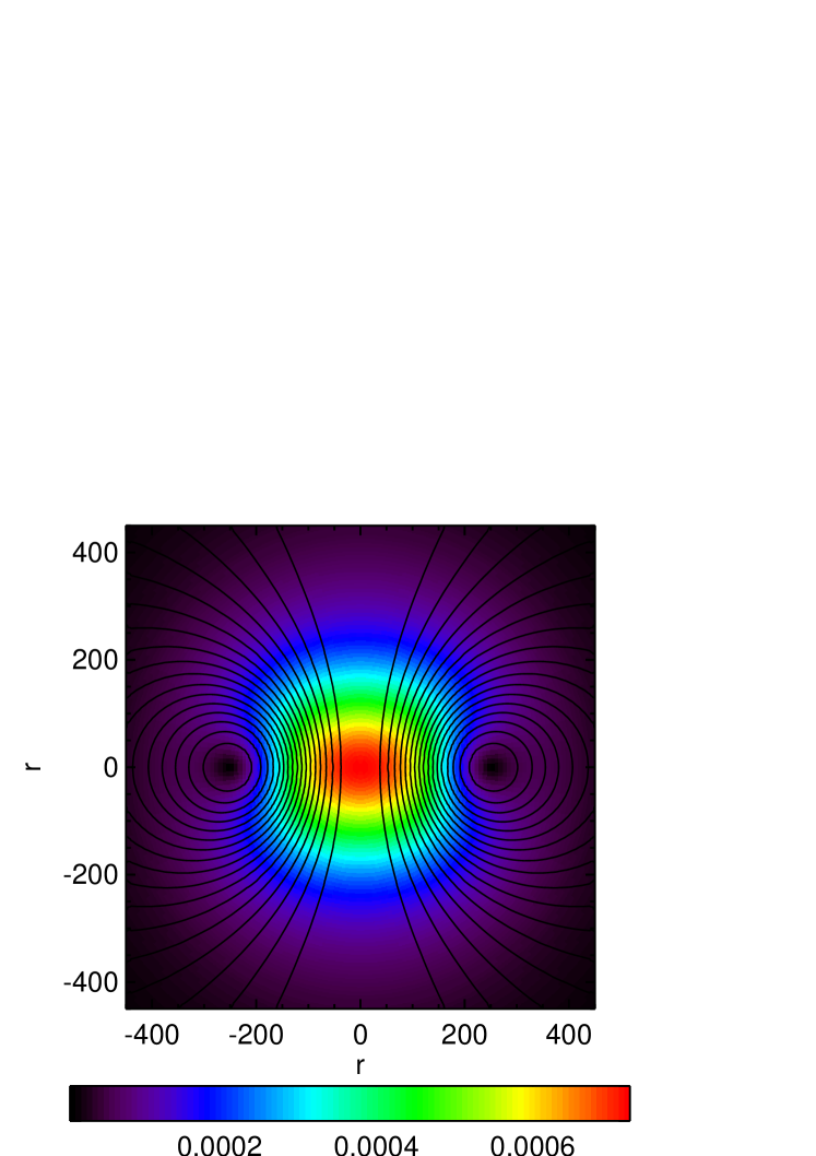
Figure 1: Illustration of poloidal magnetic field geometries, when the black contours are the magnetic surfaces. The field is in units of $10^{14}$ G and $r$ is in units of 1.48km.

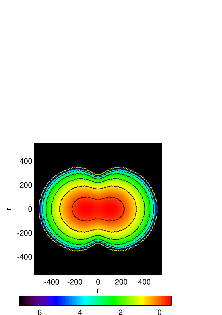
Figure 2: The contour plots of density in logarithmic scale, when density is in units of $10^{10}$ gm/cc for differentially rotating white dwarfs having poloidal magnetic fields with $M=1.95M_{\odot}$, equatorial radius $746$ km, the ratio of polar to equatorial radii $0.564$.

Table 2: Differentially rotating configurations having purely toroidal magnetic field, with changing maximum magnetic field $B_{max}$ within white dwarfs, when central angular velocity $\Omega_{c}=30.42$ sec^-1 fixed. $r_{e}$ and $r_{p}$ are respectively the equatorial and polar radii.

$B_{max}(10^{14}~{}{\rm G})$	$M(M_{\odot})$	$r_{e}({\rm km})$	$\Omega_{eq}({\rm sec^{-1}})$	KE/GE	ME/GE	$r_{p}/r_{e}$
0	1.769	1410	2.990	0.126	0	0.613
2.299	1.959	1676	2.180	0.132	0.046	0.603
2.996	2.318	2171	1.339	0.136	0.108	0.583
3.584	3.159	3322	0.593	0.132	0.203	0.584

4.2 Modified General Relativity

Magnetized white dwarfs are unable to explain the under-luminous SNeIa mentioned above. There are however some proposed models, with caveats, to describe them. For example, numerical simulations of the merger of two sub-Chandrasekhar white dwarfs reproduce the low power of under-luminous SNeIa, however the simulated light-curves fade slower than that suggested by observations.

A major concern, however, is that a large array of models is required to explain apparently the same phenomena, i.e., triggering of thermonuclear explosions in white dwarfs. Why nature would seek mutually uncorrelated scenarios to exhibit sub- and super-SNeIa? This is where the idea of modifying GR steps in into the context of white dwarfs, which unifies the sub-classes of SNeIa by a single underlying theory.

Let me consider, for the present purpose, the simplistic Starobinsky model [9] defined as $f(R)=R+\alpha R^{2}$, when $\alpha$ is a constant. However, similar effects could also be obtained in other, physically more sophisticated, theories, where $\alpha$ (or effective-$\alpha$) is varying (e.g., with density). Now, on extremizing the action equation (1) for Starobinsky’s model, one obtains the modified field equation of the form

$$G_{\mu\nu}+\alpha X_{\mu\nu}=\frac{8\pi GT_{\mu\nu}}{c^{4}},$$ (6)

where $T_{\mu\nu}$ contains only the matter field (non-magnetic star) and $X_{\mu\nu}$ is a function of $g_{\mu\nu}$, $R_{\mu\nu}$ and $R$ (see [52] for details).

Here, I seek perturbative solutions of equation (6) (see, e.g., [10]), such that $\alpha R\ll 1$. Furthermore, I consider the hydrostatic equilibrium condition so that $g_{\nu r}\nabla_{\mu}T^{\mu\nu}=0$, with zero velocity and $\nabla_{\mu}$ the covariant derivative. Hence, I obtain the differential equations for mass $M_{\alpha}(r)$, pressure $P_{\alpha}(r)$ (or density $\rho_{\alpha}(r)$) and gravitational potential $\phi_{\alpha}(r)$, of spherically symmetric white dwarfs (which is basically the set of modified Tolman-Oppenheimer-Volkoff (TOV) equations). For $\alpha=0$, these equations reduce to TOV equations in GR.

I supply EoS, obtained by Chandrasekhar [53], as $P_{0}=K\rho_{0}^{1+(1/n)}$, where $P$ and $\rho$ of Ref. 53 are replaced by $P_{0}$ and $\rho_{0}$ respectively ($\alpha=0$: GR) in the spirit of perturbative approach. This form of EoS is valid for extremely low and high densities, where $n$ is the polytropic index and $K$ a dimensional constant. The boundary conditions are: $M_{\alpha}(0)=0$ and $\rho_{\alpha}(0)=\rho_{c}$, where $\rho_{c}$ is the central density of the white dwarf. Note that a particular $\rho_{c}$ corresponds to a particular $M_{\alpha}$ and radius $R_{\alpha}$ of white dwarfs. Hence, by varying $\rho_{c}$ from $2\times 10^{5}$ gm/cc to $10^{11}$ gm/cc, I construct the mass-radius relation.

Figures 1(a) and 1(b) show that all three $M_{\alpha}-\rho_{c}$ curves for $\alpha<0$ overlap with the $\alpha=0$ curve in the low density region. However, with the increase of $\alpha$, the region of overlap recedes to a lower $\rho_{c}$. Modified GR effects become important and visible at $\rho_{c}\gtrsim 10^{8},~{}4\times 10^{7}$ and $2\times 10^{6}$ gm/cc, for $\alpha=2\times 10^{13}~{}{\rm cm^{2}}$, $8\times 10^{13}~{}{\rm cm^{2}}$ and $10^{15}~{}{\rm cm^{2}}$ respectively. For a given $\alpha$, with the increase of $\rho_{c}$, $M_{\alpha}$ first increases, reaches a maximum and then decreases, like the $\alpha=0$ (GR) case. With the increase of $\alpha$, maximum mass $M_{\rm max}$ decreases and for $\alpha=10^{15}~{}{\rm cm}^{2}$ it is highly sub-Chandrasekhar ($0.81M_{\odot}$). This reveals that modified GR has a tremendous impact on white dwarfs. In fact, $M_{\rm max}$ for all the chosen $\alpha>0$ is sub-Chandrasekhar, ranging $1.31-0.81M_{\odot}$. This is a remarkable finding since it establishes that even if $\rho_{c}$s for these sub-Chandrasekhar white dwarfs are lower than the conventional value at which SNeIa are usually triggered, an attempt to increase the mass beyond $M_{\rm max}$ with increasing $\rho_{c}$ will lead to a gravitational instability. This presumably will be followed by a runaway thermonuclear reaction, provided the core temperature increases sufficiently due to collapse. Occurrence of such thermonuclear runway reactions, triggered at densities as low as $10^{6}$ gm/cc, has already been demonstrated [54]. Thus, once $M_{\rm max}$ is approached, a SNIa is expected to trigger just like in the $\alpha=0$ case, explaining the sub-SNeIa [43, 44], like SN 1991bg mentioned above.

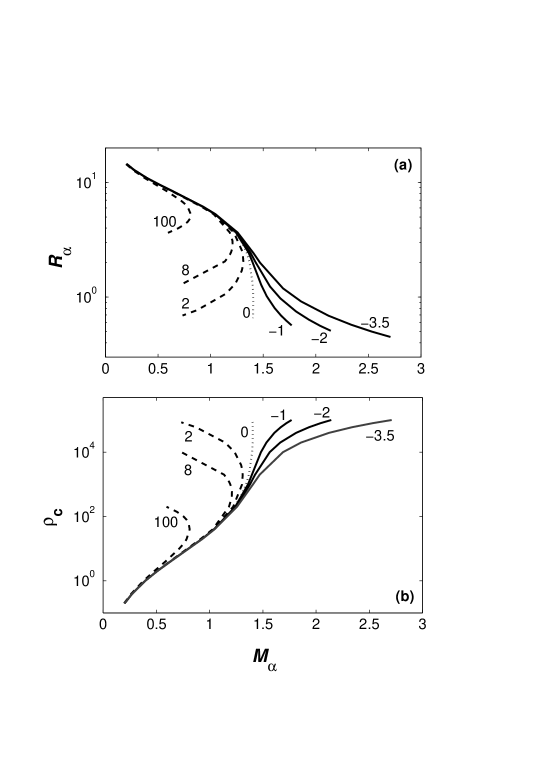
Figure 3: Unification diagram for SNeIa: (a) mass-radius relations, (b) variation of $\rho_{c}$ with $M_{\alpha}$. The numbers adjacent to the various lines denote $\alpha/(10^{13}~{}{\rm cm^{2}})$. $\rho_{c}$, $M_{\alpha}$ and $R_{\alpha}$ are in units of $10^{6}$ gm/cc, $M_{\odot}$ and 1000 km respectively.

For $\alpha<0$ cases, Fig. 1(b) shows that for $\rho_{c}>10^{8}$ gm/cc, the $M_{\alpha}-\rho_{c}$ curves deviate from the GR curve due to modified GR effects. Note that $M_{\rm max}$ for all the three cases corresponds to $\rho_{c}=10^{11}$ gm/cc, an upper-limit chosen to avoid possible neutronization. Interestingly, all values of $M_{\rm max}$ are highly super-Chandrasekhar, ranging from $1.8-2.7M_{\odot}$. Thus, while the GR effect is very small, modified GR effect could lead to $\sim 100\%$ increase in the limiting mass of white dwarfs. The corresponding values of $\rho_{c}$ are large enough to initiate thermonuclear reactions, e.g. they are larger than $\rho_{c}$ corresponding to $M_{\rm max}$ of $\alpha=0$ case, whereas the respective core temperatures are expected to be similar. This explains the entire range of the observed super-SNeIa mentioned above [41, 42], assuming the furthermore gain of mass above $M_{\rm max}$ leads to SNeIa.

Tables 2 and 3 ensure the perturbative validity of the solutions. Recall that I solve the modified TOV equations only up to ${\cal O}(\alpha)$. Since the product $\alpha R$ is first order in $\alpha$, I replace $R$ in it by the zero-th order Ricci scalar $R^{(0)}=8\pi(\rho^{(0)}-3P^{(0)})$, which is Ricci scalar obtained in GR ($\alpha=0$). For the perturbative validity of the entire solution, $|\alpha R^{(0)}|_{\rm max}\ll 1$ should hold true. Next, I consider $g_{tt}^{(0)}/g_{tt}$ and $g_{rr}^{(0)}/g_{rr}$ (ratios of $g_{\mu\nu}$-s in GR and those in modified GR up to ${\cal O}(\alpha)$), which should be close to unity for the validity of perturbative method [55]. Hence, $|1-g_{tt}^{(0)}/g_{tt}|_{\rm max}\ll 1$ and $|1-g_{rr}^{(0)}/g_{rr}|_{\rm max}\ll 1$ should both hold true. Tables 2 and 3 indeed show that all the three measures quantifying perturbative validity are at least $2-3$ orders of magnitude smaller than 1.

Table 3: Measure of validity of perturbative solutions for $\alpha>0$ corresponding to $M_{\rm max}$ in Fig. 3.

$\alpha/(10^{13}~{}{\rm cm}^{2})$	$|\alpha R^{(0)}|_{\rm max}$	$|1-g^{(0)}_{tt}/g_{tt}|_{\rm max}$	$|1-g^{(0)}_{rr}/g_{rr}|_{\rm max}$
2	$7.4\times 10^{-5}$	$6.8\times 10^{-5}$	$2.0\times 10^{-4}$
8	$7.4\times 10^{-5}$	$6.8\times 10^{-5}$	$2.0\times 10^{-4}$
100	$7.4\times 10^{-5}$	$6.9\times 10^{-5}$	$2.0\times 10^{-4}$

Table 4: Measure of validity of perturbative solutions for $\alpha<0$ corresponding to $M_{\rm max}$ in Fig. 3.

$\alpha/(10^{13}~{}{\rm cm}^{2})$	$|\alpha R^{(0)}|_{\rm max}$	$|1-g^{(0)}_{tt}/g_{tt}|_{\rm max}$	$|1-g^{(0)}_{rr}/g_{rr}|_{\rm max}$
-1	0.00184	0.0016	0.0052
-2	0.00369	0.0031	0.0108
-3.5	0.00646	0.0052	0.0199

4.2.1 Possible effect of density dependent model parameter leading to chameleon-like theory

I now justify that the effects of modified GR based on a more sophisticated calculation, invoking an (effective) $\alpha$ that varies explicitly with density (and effectively becomes negative), are likely to converge to those described above with constant $\alpha$. Note that even though $\alpha$ is assumed to be constant within individual white dwarfs here, there is indeed an implicit dependence of $\alpha$ on $\rho_{c}$, particularly of the liming mass white dwarfs presumably leading to SNeIa, as is evident from Fig. 3(b). This indicates the existence of an underlying chameleon effect. This trend is expected to emerge self-consistently in a varying-$\alpha$ theory.

Let me consider a possible situation where $\alpha$ varies explicitly with density and try to relate it with the above results. Note that the super-SNeIa occur mostly in young stellar populations consisting of massive stars (see, e.g., [41]), while the sub-SNeIa occur in old stellar populations consisting of low mass stars (see, e.g., [56]). The massive stars with higher densities are likely to collapse to give rise to super-Chandrasekhar white dwarfs, which would subsequently explode to produce super-SNeIa. The low mass stars with lower densities would be expected to collapse to give rise to sub-Chandrasekhar white dwarfs, which would probably end in sub-SNeIa. Now, let me assume a functional dependence of $\alpha$ on density such that there are two terms — one dominates at higher densities, while the other dominates at lower densities. Hence, when a massive, high density star collapses, it yields results similar to our $\alpha<0$ cases; while when a low mass, low density star collapses, it leads to results like our $\alpha>0$ cases. Thus, the same functional form of $\alpha$ could lead to both super- and sub-Chandrasekhar limiting mass white dwarfs, respectively. Note that the final mass of the white dwarf would depend on several factors, such as, $\rho_{c}$ and the density gradient in the parent star, etc. Interestingly, this description invoking a variation of $\alpha$ with density is essentially equivalent to invoking a so-called “chameleon-$f(R)$ theory”, which can pass solar system tests of gravity (see, e.g., [57]). This is so because $\alpha$ is a function of density, which in turn is a function of $R$ and, hence, introducing a density (and hence $R$) dependence into $\alpha$ is equivalent to choosing an appropriate (more complicated) $f(R)$ model of gravity. Therefore, even when one invokes a more self-consistent variation of $\alpha$ with density, it does not invalidate the results of the constant-$\alpha$ cases, rather is expected to complement the picture.

On a related note, I would like to mention that the order of magnitude of $\alpha$ is different between that in typical white dwarfs ($\alpha\sim 10^{13}$ ${\rm cm^{2}}$, as used above) and in neutron stars ($\alpha\sim 10^{9}$ ${\rm cm^{2}}$, e.g. [11, 10]). This again basically stems from the fact that there is an underlying chameleon effect which causes $\alpha$ to be different in different density regimes. Note that neutron stars are much denser than white dwarfs and, hence, have a higher value of curvature $R$. Now, the quantity $\alpha R$ would have a similar value in both neutron stars and white dwarfs in the perturbative regime. Hence, due to their higher curvature, neutron stars will harbor a smaller value of $\alpha$ compared to white dwarfs. Roughly, neutron stars are $10^{4}$ times denser than white dwarfs and, hence, $\alpha_{neutron-star}$ is $10^{4}$ times smaller than $\alpha_{white-dwarf}$.

5 Summary

In the last several decades, relativistic astrophysics has turned out to be a highly important branch in astrophysics. In this branch, many major astrophysical discoveries are still taking place in the contexts of black holes, quasars, neutron stars, white dwarfs, X-ray binaries, gamma-ray bursts, particle acceleration, the cosmic background, dark matter, dark energy etc., even 100 years after Einstein’s discovery of GR, which is the basic building block for them. The present article has touched upon some of the underlying latest astrophysical problems and their possible resolutions. It has been revealed that while Einstein’s gravity itself is indispensable to uncover modern high energy astrophysical problems, modified Einstein’s gravity also appears to be playing an important role behind certain phenomena and, in general, to explain astrophysical processes.

Acknowledgment

I am thankful to Indrani Banerjee, Mukul Bhattacharya, Upasana Das, Chanda J. Jog, Subroto Mukerjee, A. R. Rao, Prateek Sharma and Sathyawageeswar Subramanian, for continuous discussions on the topics covered in this article.

References

- [1] A. Einstein, SPAW, 844 (1915).
- [2] K. Schwarzschild, AbhKP, 189 (1916).
- [3] R. Kerr, Phys. Rev. Lett. 11, 237 (1963).
- [4] R. H. Boyer, & R. W. Lindquist, JMP 8, 265 (1967).
- [5] J. B. Hartle, & K. S. Thorne, ApJ 153, 807 (1968).
- [6] G. B. Cook, S. L. Shapiro, & S. A. Teukolsky, ApJ 424, 823 (1994).
- [7] N. Bucciantini, & L. Del Zanna, A&A 528, A101 (2011).
- [8] R. A. Hulse, & J. H. Taylor, ApJ 195, 51 (1975).
- [9] A. A. Starobinsky, Phys. Lett. B 91, 99 (1980).
- [10] A. V. Astashenok, S. Capozziello and S. D. Odintsov, JCAP 12, 040 (2013).
- [11] S. Arapoğlu, C. Deliduman, & K. Y. Ekşi, JCAP 7, 020 (2011).
- [12] P. B. Demorest, et al., Nature 467, 1081 (2010).
- [13] J. Antoniadis, et al., Science 340, 448 (2013).
- [14] S. Weissenborn, D. Chatterjee, & J. Schaffner-Bielich, Phys. Rev. C 85, 065802 (2012).
- [15] D. L. Whittenbury, J. D. Carroll, A. W. Thomas, K. Tsushima, & J. R. Stone, Phys. Rev. C. 89, 065801 (2014).
- [16] A. G. Pili, N. Bucciantini, & L. Del Zanna, MNRAS 439, 3541 (2014).
- [17] M.-K. Cheoun, C. Deliduman, C. Gungor, V. Keles, C. Y. Ryu, T. Kajino, & G. J. Mathews, JCAP 10, 021 (2013).
- [18] H. Bondi, MNRAS 112, 195 (1952).
- [19] F. C. Michel, Ap&SS 15, 153 (1972).
- [20] I. D. Novikov, & K. S. Thorne, in Black Holes, ed. C. DeWitt & B. S. DeWitt (New York: Gordon and Breach), 343 (1973).
- [21] N. I. Shakura, R. A. Sunyaev, A&A 24, 366 (1973).
- [22] S. L. Shapiro, A. P. Lightman, & D. M. Eardley, ApJ 204, 187 (1976).
- [23] R. Narayan, I. Yi, ApJ 428, L13 (1994).
- [24] B. Paczyńsky, & P. J. Wiita, A&A 88, 23 (1980).
- [25] B. Mukhopadhyay, ApJ 581, 427 (2002).
- [26] E. P. T. Liang, & K. A. Thompson, ApJ 240, 271 (1980).
- [27] S. K. Chakrabarti, ApJ 350, 275 (1990).
- [28] C. F. Gammie, & R. Popham, ApJ 498, 313 (1998).
- [29] W.-X. Chen, & A. M. Beloborodov, ApJ 657, 383 (2007).
- [30] A. Tchekhovskoy, R. Narayan, & J. C. McKinney, MNRAS 418, 79 (2011).
- [31] J. C. McKinney, A. Tchekhovskoy, & R. D. Blandford, MNRAS 423, 3083 (2012).
- [32] J. C. McKinney, A. Tchekhovskoy, A. Sadowski, & R. Narayan, MNRAS 441, 3177 (2014).
- [33] A. de Felice, & S. Tsujikawa, Liv. Rev. Rel. 13, 3 (2010).
- [34] J. E. McClintock, at al., CQG 28, 114009 (2011).
- [35] R. C. Reis, A. C. Fabian, R. R. Ross, & J. M. Miller, MNRAS 395, 1257 (2009).
- [36] B. Mukhopadhyay, ApJ 694, 387 (2009).
- [37] B. Mukhopadhyay, D. Bhattacharya, & P. Sreekumar, IJMPD 21, 1250086 (2012).
- [38] I. Banerjee, & B. Mukhopadhyay, Phys. Rev. Lett. 111, 061101 (2013).
- [39] S. W. Davis, & A. Laor, ApJ 728, 98 (2011).
- [40] S. Perlmutter, et al., Astrophys. J. 517, 565 (1999).
- [41] D. A. Howell, et al., Nature 443, 308 (2006).
- [42] R. A. Scalzo, et al., Astrophys. J. 713, 1073 (2010).
- [43] A. V. Filippenko, et al., Astron. J. 104, 1543 (1992).
- [44] S. Taubenberger, et al., Mon. Not. R. Astron. Soc. 385, 75 (2008).
- [45] U. Das, & B. Mukhopadhyay, Phys. Rev. D 86, 042001 (2012).
- [46] U. Das, & B. Mukhopadhyay, Phys. Rev. Lett. 110, 071102 (2013).
- [47] U. Das, & B. Mukhopadhyay, JCAP 06, 050 (2014).
- [48] U. Das, & B. Mukhopadhyay, JCAP 05, 016 (2015).
- [49] A. G. Pili, N. Bucciantini, & L. Del Zanna, MNRAS 439, 3541 (2014).
- [50] J. P. Ostriker, & F. D. A. Hartwick, ApJ 153, 797 (1968).
- [51] S. Subramanian, & B. Mukhopadhyay, MNRAS 454, 752 (2015).
- [52] U. Das, & B. Mukhopadhyay, JCAP 05, 045 (2015).
- [53] S. Chandrasekhar, MNRAS 95, 207 (1935).
- [54] I. R. Seitenzahl, C. A. Meakin, D. M. Townsley, D. Q. Lamb, & J. W. Truran, ApJ 696, 515 (2009).
- [55] M. Orellana, F. García, F. A. Teppa Pannia, & G. E. Romero, Gen. Rel. Grav. 45, 771 (2013).
- [56] S. González-Gaitán, et al., ApJ 727, 107 (2011).
- [57] T. Faulkner, M. Tegmark, E. F. Bunn, Y. Mao, Phys. Rev. D 76, 063505 (2007).