Angular momentum evolution of galaxies in EAGLE

Abstract

We use the eagle cosmological hydrodynamic simulation suite to study the specific angular momentum of galaxies, $j$, with the aims of (i) investigating the physical causes behind the wide range of $j$ at fixed mass and (ii) examining whether simple, theoretical models can explain the seemingly complex and non-linear nature of the evolution of $j$. We find that $j$ of the stars, $j_{\rm stars}$, and baryons, $j_{\rm bar}$, are strongly correlated with stellar and baryon mass, respectively, with the scatter being highly correlated with morphological proxies such as gas fraction, stellar concentration, (u-r) intrinsic colour, stellar age and the ratio of circular velocity to velocity dispersion. We compare with available observations at $z=0$ and find excellent agreement. We find that $j_{\rm bar}$ follows the theoretical expectation of an isothermal collapsing halo under conservation of specific angular momentum to within $\approx 50$%, while the subsample of rotation-supported galaxies are equally well described by a simple model in which the disk angular momentum is just enough to maintain marginally stable disks. We extracted evolutionary tracks of the stellar spin parameter of eagle galaxies and found that the fate of their $j_{\rm stars}$ at $z=0$ depends sensitively on their star formation and merger histories. From these tracks, we identified two distinct physical channels behind low $j_{\rm stars}$ galaxies at $z=0$: (i) galaxy mergers, and (ii) early star formation quenching. The latter can produce galaxies with low $j_{\rm stars}$ and early-type morphologies even in the absence of mergers.

1 Introduction

The formation of galaxies can be a highly non-linear process, with many physical mechanisms interacting simultaneously (see reviews by Baugh 2006; Benson 2010). Notwithstanding all that potential complexity, early studies of galaxy formation stressed the importance of three quantities to describe galaxies: mass, $M$, angular momentum, $J$, and energy, $E$ (Peebles, 1969; Doroshkevich, 1970; Fall & Efstathiou, 1980; White, 1984); or alternatively, one can define the specific angular momentum, $j\equiv J/M$, which contains information on the scale length and rotational velocity of systems. It is therefore intuitive to expect the relation between $j$ and $M$ to contain fundamental information.

Studies such as Fall & Efstathiou (1980), White & Frenk (1991), Catelan & Theuns (1996a) and Mo et al. (1998), showed that many properties of galaxies, such as flat rotation curves, and the Tully-Fisher relation could be obtained in the Cold Dark Matter (CDM) framework if $j$ of baryons is similar to that of the halo and is conserved in the process of disk formation (although conservation does not need to be strict, but within a factor of $\approx 2$; Fall 1983). The situation is of course different for the mass and energy of galaxies, which can vary significantly throughout their evolution due to accretion, star formation and dissipative processes, such as galaxy mergers. Theoretical models of how $j$ of halos evolves in a CDM universe predict $j\propto\lambda\,M^{2/3}$, where $\lambda$ is the spin parameter of the halo (e.g. White 1984; Catelan & Theuns 1996a; Mo et al. 1998). If $j$ of baryons is conserved throughout the formation of galaxies, then a similar relation should apply to galaxies. These models generally assume that halos collapse as their spherical overdensity reaches a threshold value, and in that sense neglect mergers. Due to the dissipative nature of the latter, one would expect significant changes in the relation between $j$ and $M$ of halos and galaxies (Zavala et al., 2008; Sales et al., 2012; Romanowsky & Fall, 2012).

Hydrodynamic simulations used to suffer from catastrophic loss of angular momentum, producing galaxies that were too compact and too low $j$ compared to observations (Steinmetz & Navarro, 1999; Navarro & Steinmetz, 2000). This problem was solved by improving the spatial resolution and including efficient feedback (e.g. Kaufmann et al. 2007; Zavala et al. 2008; Governato et al. 2010; Guedes et al. 2011; Danovich et al. 2015). A new generation of simulations have immensely improved in spatial resolution, volume and sophistication of the sub-grid physics included, allowing the study of angular momentum loss in galaxies statistically. For example, simulations such as eagle (Schaye et al., 2015), Illustris (Vogelsberger et al., 2014) and Horizon-AGN (Dubois et al., 2014) achieve spatial resolutions of $\approx 700\,\rm pc$ (physical units), volumes of $(100\,\rm Mpc)^{3}$, and include models for metal cooling, star formation and stellar and active galactic nucleus (AGN) feedback. These simulations contain thousands of galaxies with stellar masses $>10^{10}\,\rm M_{\odot}$.

Observationally, Fall (1983) presented the first study of the relation between $j$ of the stellar component, $j_{\rm stars}$, and stellar mass. Fall (1983) found that both spiral and elliptical galaxies follow a relation that is close to $j\propto M^{2/3}$, but with spiral galaxies having a normalisation $\approx 5$ times larger than elliptical galaxies. Recently, this was extended by Romanowsky & Fall (2012) and Fall & Romanowsky (2013) in a sample of $\approx 100$ galaxies. These studies confirmed that the power-law index of the relation was close to $2/3$ for their entire galaxy population and that ellipticals galaxies had significantly lower $j$ than spiral galaxies at a given mass.

Obreschkow & Glazebrook (2014) presented the most accurate measurements of $j$ in the stellar, neutral gas and total baryon components of galaxies out to large radii ($\approx 10$ times the disk scale length) in a sample of $16$ late-type galaxies of the HI Nearby Galaxy Survey (THINGS; Walter et al. 2008) and found (i) galaxies follow a relation close to $j_{\rm stars}\propto M^{2/3}_{\rm stars}$ and $j_{\rm bar}\propto M^{2/3}_{\rm bar}$, where $M_{\rm stars}$, $M_{\rm bar}$ and $j_{\rm bar}$ are the stellar mass, baryon mass (stars plus neutral gas) and baryon specific angular momentum respectively, (2) the scatter in the $j_{\rm bar}$-$M_{\rm bar}$ and $j_{\rm stars}$-$M_{\rm stars}$ relations is strongly correlated with the bulge-to-total stellar mass ratio and the neutral gas fraction (neutral mass divided by baryon mass; $f_{\rm gas,neutral}$). By fixing the bulge-to-total stellar mass ratio, Obreschkow & Glazebrook (2014) found that $j_{\rm bar}\propto M_{\rm bar}$. Using the Toomre (1964) stability model, surface density of the gas in galaxies and a flat exponential disk, Obreschkow et al. (2016) found that the atomic gas fraction in galaxies is $\propto(j_{\rm bar}/M_{\rm bar})^{1.12}$. Obreschkow & Glazebrook (2014) argued that under the assumption that bulges in spiral galaxies form through disk instabilities, one could understand the relation between $j_{\rm stars}$, stellar mass and bulge-to-total stellar mass ratio from the model above. Stevens et al. (2016a), using a semi-analytic model, showed that disk instabilities play a major role in regulating the $j_{\rm stars}-M_{\rm stars}$ sequence for spiral galaxies, consistent with the picture of Obreschkow & Glazebrook (2014).

To measure $j$ accurately in galaxies, requires spatially resolved kinematic information. The pioneering work of the SAURON (Bacon et al., 2001) and ATLAS^3D (Cappellari et al., 2011a) surveys, on samples of galaxies that comprised $260$ early-type galaxies in total, showed that the stellar kinematics and distributions of stars are not strongly correlated, and thus morphology is not necessarily a good indicator of the dynamics of galaxies (Krajnović et al., 2013a). Based on these surveys, Emsellem et al. (2007, 2011) coined the terms slow and fast rotators, and proposed the $\lambda_{\rm R}$ parameter, which measures how rotationally or dispersion-dominated a galaxy is and is closely connected to $j_{\rm stars}$, as a new, improved scheme to classify galaxies. Naab et al. (2014) showed later that such a classification is also applicable for galaxies in hydrodynamic simulations. Unfortunately, accurate measurements of $j$ have only been presented for a few hundred galaxies. The future, however, is bright: the advent of integral field spectroscopy (IFS) and the new generation of radio and millimeter telescopes promises a revolution in the field.

Currently, the Sydney-AAO Multi-object Integral field spectrograph (SAMI; Croom et al. 2012) survey is observing $\approx 3,200$ galaxies for which resolved kinematics will be available (Bryant et al., 2015). Similarly, high-resolution radio telescopes, such as the Square Kilometre Array (SKA), promise to collect information that would allow the measurement of $j$ for few thousand galaxies during its first years (Obreschkow et al., 2015), truly revolutionising our understanding of the build-up of angular momentum in galaxies. Cortese et al. (2016) presented the first measurements of the $j_{\rm stars}$-$M_{\rm stars}$ relation for $297$ galaxies in SAMI, and found that, for the entire sample and for a relation of the form $j_{\rm stars}\propto M^{\alpha}_{\rm stars}$, $\alpha\approx 0.7$, close to the theoretical expectation of $2/3$, but when studied in subsamples of different morphological types $\alpha$ varies from $0.69$ for elliptical galaxies to $0.97$ for spiral galaxies. Cortese et al. found that the dispersion of the $j_{\rm stars}-M_{\rm stars}$ relation is correlated with morphological proxies such as Sérsic index and light concentration. These new results have not yet been examined in simulations.

In this paper we explore two long-standing open questions of how $j$ evolves in galaxies: (i) how does $j$ depend with mass, and what are the most relevant secondary galaxy properties, and (ii) how well do simple, theoretical models explain the evolution of $j$ in a complex, non-linear hydrodynamical simulations. In our opinion, eagle is the ideal testbed for this experiment due to the spatial resolution achieved, the large volume that allows us to statistically assess these relations and also the growing amount of evidence that the simulation produces a realistic galaxy population. For instance, eagle reproduces well the relations between star formation rate (SFR) and stellar mass (Furlong et al. 2015b; Schaye et al. 2015), the colour bi-modality of galaxies (Trayford et al. 2015, 2016), the molecular and atomic gas fractions as a function of stellar mass (Lagos et al. 2015; Bahé et al. 2016; Crain et al. 2016), and the co-evolution of stellar mass, SFR and gas (Lagos et al., 2016).

So far, simulations have been used to test theoretical models for the evolution of angular momentum. For instance, Zavala et al. (2016) presented a study of the build-up of angular momentum of the stars, cold gas and dark matter in eagle, and showed that disks form mainly after the turnaround epoch (epoch of maximum expansion of halos, after which they collapse into virialised structures, approximately conserving specific angular momentum) while bulges formed before turnaround, explaining why bulges have much lower $j$. Zavala et al. (2016) also compared the $j_{\rm stars}$-$M_{\rm stars}$ relation for eagle galaxies at $z=0$ with the observations of Romanowsky & Fall (2012) and found general agreement. Teklu et al. (2015) and Pedrosa & Tissera (2015) also found that that the positions of galaxies in the $j_{\rm stars}$-$M_{\rm stars}$ relation is correlated with the bulge-to-total stellar mass ratio in the Magneticum and Fornax simulations, respectively. Similarly, Genel et al. (2015) presented an analysis of the effect of baryon processes on the $j_{\rm stars}$-$M_{\rm stars}$ relation in the Illustris simulation and confirmed previous results that feedback is a key process preventing catastrophic angular momentum loss. Here we investigate several galaxy properties that have been theoretically and/or empirically proposed to be relevant for the relationship between $j$ and mass in eagle, and extend previous work by exploring a larger parameter space of galaxy properties that could determine the positions of galaxies in the $j$-mass relation of different baryonic components of galaxies. We also perform the most, to our knowledge, comprehensive comparison between hydrodynamic simulations and observations of $j$ to date.

This paper is organised as follows. In $\S$ 2 we give a brief overview of the simulation, and describe how the dynamic and kinematic properties of galaxies used in this paper are calculated. In $\S$ 3 we give a theoretical background that we then use to interpret our results. In $\S$ 4 we explore the dependence of $j$ on galaxy properties at $z=0$ and present a comprehensive comparison with observations. In $\S$ 5 we analyse in detail the evolution of $j$ of the different baryonic components of galaxies, and identify average evolutionary tracks of $j_{\rm stars}/M^{2/3}_{\rm stars}$. Here we also compare the evolution of $j$ in eagle with simple, theoretical models to study how closely these models can reproduce the trends seen in eagle. We discuss our results and present our conclusions in $\S$ 6. In Appendix A we present ‘weak’ and ‘strong’ convergence tests (terms introduced by Schaye et al. 2015), and in Appendix B we present additional scaling relations between the specific angular momentum of stars and baryons and other galaxy properties.

2 The EAGLE simulation

Table 1: Features of the Ref-L100N1504 simulation used in this paper. The row list: (1) comoving box size, (2) number of particles, (3) initial particle masses of gas and (4) dark matter, (5) comoving gravitational softening length, and (6) maximum physical comoving Plummer-equivalent gravitational softening length. Units are indicated in each row. eagle adopts (5) as the softening length at $z\geq 2.8$, and (6) at $z<2.8$.

	Property	Units	Value
(1)	$L$	$[\rm cMpc]$	$100$
(2)	# particles		$2\times 1504^{3}$
(3)	gas particle mass	$[\rm M_{\odot}]$	$1.81\times 10^{6}$
(4)	DM particle mass	$[\rm M_{\odot}]$	$9.7\times 10^{6}$
(5)	Softening length	$[\rm ckpc]$	$2.66$
(6)	max. gravitational softening	$[\rm pkpc]$	$0.7$

The eagle simulation suite (described in detail by Schaye et al. 2015, hereafter S15, and Crain et al. 2015, hereafter C15) consists of a large number of cosmological hydrodynamic simulations with different resolutions, cosmological volumes and subgrid models, adopting the Planck Collaboration (2014) cosmological parameters. S15 introduced a reference model, within which the parameters of the sub-grid models governing energy feedback from stars and accreting black holes (BHs) were calibrated to ensure a good match to the $z=0.1$ galaxy stellar mass function and the sizes of present-day disk galaxies.

In Table 1 we summarise the parameters of the simulation used in this work, including the number of particles, volume, particle masses, and spatial resolution. Throughout the text we use pkpc to denote proper kiloparsecs and cMpc to denote comoving megaparsecs. A major aspect of the eagle project is the use of state-of-the-art sub-grid models that capture unresolved physics. The sub-grid physics modules adopted by eagle are: (i) radiative cooling and photoheating, (ii) star formation, (iii) stellar evolution and enrichment, (iv) stellar feedback, and (v) black hole growth and active galactic nucleus (AGN) feedback (see S15 for details on how these are modelled and implemented in eagle). In addition, the fraction of atomic and molecular gas in gas particle is calculated in post-processing following Lagos et al. (2015).

The eagle simulations were performed using an extensively modified version of the parallel $N$-body smoothed particle hydrodynamics (SPH) code gadget-3 (Springel et al. 2008; Springel 2005). Among those modifications are updates to the SPH technique, which are collectively referred to as ‘Anarchy’ (see Schaller et al. 2015 for an analysis of the impact of these changes on the properties of simulated galaxies compared to standard SPH). We use SUBFIND (Springel et al. 2001; Dolag et al. 2009) to identify self-bound overdensities of particles within halos (i.e. substructures). These substructures are the galaxies in eagle.

2.1 Calculation of dynamic and kinematic properties of galaxies in EAGLE

Here we describe how we measure velocity dispersion of the stars; specific angular momentum and the stellar, neutral gas (atomic and molecular gas mass, in both components hydrogen plus helium) and total baryon components; rotational velocity; and $\lambda_{\rm R}$ parameters. We measure these properties in apertures that range from $3$ pkpc to $500$ pkpc in all galaxies with $M_{\rm stars}>10^{9}\,\rm M_{\odot}$. We also calculate the half-mass radius of stars, which we use to compute $j$ of the stellar component in a physically meaningful aperture, which is also comparable to those used in observations.

We calculate the $1$-dimensional velocity dispersion of the stars perpendicular to the midplane of the disk. We do this by calculating the velocity relative to the centre of mass $\Delta v_{\rm i}=\mid\vec{v}_{\rm i}-\vec{v}_{\rm COM}\mid$. Here, $\vec{v}_{i}$ and $\vec{v}_{\rm COM}$ are the velocity vectors of the $i$-th particle and that of the centre of mass, with the latter being calculated using all the particles of the subhalo (DM plus baryons). We then take the component of the velocity vector above parallel to the total stellar angular momentum vector (i.e. using all the star particles in the sub-halo), $L_{\rm stars}$, and compute:

$$\sigma_{\rm 1D,\star}(r)=\sqrt{\frac{\sum_{\rm i}\,m_{\rm i}\,(\Delta v_{\rm i}\,{\rm cos(\theta_{\rm i})})^{2}}{\sum_{\rm i}\,m_{\rm i}}}.$$ (1)

Here, $\rm cos(\theta_{\rm i})=\Delta\vec{v}_{\rm i}\cdot\vec{L}_{\rm stars}/\mid\Delta\vec{v}_{\rm i}\mid\,\mid\vec{L}_{\rm stars}\mid$. We calculate the rotational velocity of a galaxy from the specific angular momentum of the baryons (star and gas particles with a non-zero neutral gas fraction), $\vec{j}_{\rm bar}$, as:

$$V_{\rm rot}(r)\equiv\frac{\mid\vec{j}_{\rm bar}(r)\mid}{r}.$$ (2)

We do not include ionised gas in the calculation of $\vec{j}_{\rm bar}$ because its angular momentum is negligible compared to the stellar and neutral gas components, and because it makes it easier to compare with observations, in which this is measured from the stars, HI and H₂ (e.g. Obreschkow & Glazebrook 2014). We calculate $\vec{j}$ as

$$\vec{j}=\frac{\sum_{\rm i}\,m_{\rm i}\,(\vec{r}_{\rm i}-\vec{r}_{\rm COM})\times(\vec{v}_{\rm i}-\vec{v}_{\rm COM})}{\sum_{\rm i}\,m_{\rm i}},$$ (3)

where $\vec{r}_{\rm i}$ and $\vec{r}_{\rm COM}$ are the position vectors (from the origin of the box) of particle $i$ and the centre of mass. To calculate $j$ of the stars, neutral gas and baryons, we use star particles only, gas particles that have a non-zero neutral gas fraction only, and the latter two types of particles, respectively.

To calculate $\vec{j}(r)$, $\sigma_{\rm 1D}(r)$ and $V_{\rm rot}(r)$, we use particles enclosed in $r$. This way we avoid numerical noises due to the small number of particles that could be used if we were instead measuring these quantities in annuli. However, when we measure the $\lambda_{\rm R}$ parameter, first introduced by Emsellem et al. (2007), we need to calculate these quantities in annuli as defined in Naab et al. (2014). This parameter measures how rotationally supported a galaxy is:

$$\lambda_{\rm R}(r)=\frac{\sum^{N(r)}_{i=1}m_{\rm\star,i}\,r_{\rm i}\,V_{\rm rot}(r_{\rm i})}{\sum^{N(r)}_{i=1}m_{\rm\star,i}\,r_{\rm i}\,\sqrt{V^{2}_{\rm rot}(r_{\rm i})+\sigma^{2}_{\rm 1D,\star}(r_{\rm i})}}.$$ (4)

Here, the sum is over all the radial bins from the inner one to $r$, $N(r)$ is the number of radial bins enclosed within $r$, and $m_{\rm\star,i}$ is the stellar mass enclosed in each radial bin. This means that this quantity depends on the chosen bins. Here we choose bins of $3$ pkpc of width, to be comfortably above the resolution limits, but we tested that the higher resolution simulations return similar relations between $j_{\rm stars}-M_{\rm stars}-\lambda_{\rm R}$. Values of $\lambda_{\rm R}$ close to zero indicate dispersion-supported galaxies, while values close to $1$ indicate rotation-dominated galaxies. Typically, in observations $\lambda_{\rm R}$ has been measured within an effective radius (that encloses half of the light of a galaxy), and thus we use $\lambda_{\rm R}$ measured within a half-mass radius of the stellar component, $r_{\rm 50}$. From Eq. 4, one would expect a correlation between $j_{\rm bar}$ and $\lambda_{\rm R}$, given that $j_{\rm bar}$ appears in the nominator of Eq. 4.

Throughout the text we denote the specific angular momentum of stars as $j_{\rm stars}$ and that of the neutral gas as $j_{\rm neutral}$, unless otherwise stated, these are calculated with all the particles within $r_{\rm 50}$. The latter is a $3$-dimensional radius, rather than a projected one. This choice is made to be able to compare with observations, that usually measure $j$ within $r_{50}$. When we use ‘(tot)’, for example $j_{\rm stars}(\rm tot)$, we refer to the measurements of $j$ made using all of the particles of that class that belong to the sub-halo hosting the galaxy. In addition and unless otherwise stated, we impose $r_{\rm 50}>1$ pkpc (above the spatial resolution of the simulation), to avoid numerical artifacts.

In Appendix A we analyse the resolution limits of the simulation used here by comparing with higher resolution runs of eagle, focusing on $j_{\rm stars}$, $j_{\rm neutral}$ and $j_{\rm bar}$, as a function of stellar mass, neutral gas mass and baryon mass, respectively. We place a conservative limit in stellar, neutral gas and baryon mass above which $j_{\rm stars}$, $j_{\rm neutral}$ and $j_{\rm bar}$ are well converged (either by measuring within $r_{50}$ or within a fixed aperture). These limits are $M_{\rm stars}=10^{9.5}\,\rm M_{\odot}$, $M_{\rm bar}=10^{9.5}\,\rm M_{\odot}$ and $M_{\rm neutral}=10^{8.5}\,\rm M_{\odot}$ for the simulation used here (Table 1). Throughout the paper we show results down to stellar and baryon masses of $10^{9}\,\rm M_{\odot}$, and neutral masses of $10^{8}\,\rm M_{\odot}$, but show these conservative resolution limits to mark roughly when the results become less trustworthy.

Throughout the paper we study trends as a function of stellar, neutral gas and baryon mass. Neutral gas corresponds to the atomic plus molecular gas mass, while the baryon mass is defined as $M_{\rm bar}\equiv M_{\rm stars}+M_{\rm neutral}$ (here we neglect the ionised gas). The latter definition is close to what observations consider to be the baryon mass of galaxies (Obreschkow & Glazebrook, 2014). Following S15, all these properties are measured in $3$-dimensional apertures of $30$ pkpc. The effect of the aperture is minimal as shown by Lagos et al. (2015) and S15. Once these quantities are defined, we calculate the neutral gas fraction as:

$$f_{\rm gas,neutral}\equiv\frac{M_{\rm neutral}}{(M_{\rm neutral}+M_{\rm stars})}.$$ (5)

Note that mass measurements are close to total masses, while $j$ is measured in an aperture which is a function of $r_{50}$. We do this because in observations masses are calculated from broadband photometry, in the case of stellar mass, and from emission lines, in the case of HI and H₂ masses, that enclose the entire galaxy, which means that observations recover masses that are close to total masses. However, when $j$ is measured, high quality, resolved kinematics maps are usually required, which are in many cases only present for the inner regions of galaxies, such as within $r_{50}$.

3 Theoretical background

To interpret our findings in eagle, it is useful to set a theoretical background first, with the expectations of simple models for how $j$ evolves in galaxies under given circumstances, such as conservation of specific angular momentum. With this in mind, we introduce here the predictions of the isothermal collapsing halo model (White, 1984; Catelan & Theuns, 1996a; Mo et al., 1998) and of the more recent model of Obreschkow & Glazebrook (2014) which connects $j$ with the stability of disks and the grow of bulges.

In the model of an isothermal collapsing halo with negligible angular momentum losses, there is a relation between $j$, mass and spin parameter of the halo, $\lambda$. This relation is given by:

$$j_{\rm h}=\frac{\sqrt{2}\,G^{2/3}}{(10\,H)^{1/3}}\,\lambda\,M^{2/3}_{\rm h},$$ (6)

where $j_{\rm h}$ and $M_{\rm h}$ are the halo specific angular momentum and mass, respectively, $G$ is Newton’s gravity constant and $H$ is the Hubble parameter (Mo et al., 1998). Under the assumptions of conservation of $j$, one can write $j_{\rm bar}=j_{\rm h}$, and we can replace $M_{\rm h}$ by the baryon mass, using the baryon fraction in each halo, $M_{\rm bar}=f_{\rm b}\,M_{\rm h}$. In $\S$ 2.1 we introduced the $\lambda_{\rm R}$ parameter, and based on Emsellem et al. (2007), we can relate the halo spin with $\lambda_{\rm R}$ as $\lambda_{\rm R}\approx 10\,\lambda$ via assuming that galaxies are $\approx 10$ smaller than their halo, that $j_{\rm halo}\sim j_{\rm stars}$ and a fixed mass model (so that the relation between the gravitational and effective radii of galaxies is fixed). Kravtsov (2013) found that $r_{50}\approx 0.015\,r_{\rm halo}$, where $r_{\rm halo}$ is the halo virial radius. Obreschkow & Glazebrook (2014) showed in local spiral galaxies that $j_{\rm stars}$ and $j_{\rm bar}$ converge at $r_{\rm g}\approx 5-6\,r_{50}$, and since here we care about the total $j$, we take $r_{\rm g}\approx 0.1\,r_{\rm halo}$ as the relevant galaxy size. Using the approximations above, we can rewrite Eq. 6 in terms of the baryon component

$$j_{\rm bar}\approx\frac{\sqrt{2}\,G^{2/3}\,f^{-2/3}_{\rm b}}{10\,(10\,H)^{1/3}}\,\lambda_{\rm R}\,M^{2/3}_{\rm bar},$$ (7)

which we evaluate as

$$\frac{j_{\rm bar}}{\rm pkpc\,km\,s^{-1}}\approx 4.26\times 10^{-5}\,f^{-2/3}_{\rm b}\,\lambda_{\rm R}\,\left(\frac{M_{\rm bar}}{\rm M_{\odot}}\right)^{2/3}.$$ (8)

Eq. 8 is similar to Eq. $15$ in Romanowsky & Fall (2012), except that here we write it in terms of the baryon content and $\lambda_{\rm R}$. If for example we were to assume that $f_{\rm b}$ is constant and equal to the Universal baryon fraction measured by Planck Collaboration (2014), $f_{\rm b}=0.157$, then Eq. 8 becomes,

$$\frac{j_{\rm bar}}{\rm pkpc\,km\,s^{-1}}\approx 1.46\times 10^{-4}\,\lambda_{\rm R}\,\left(\frac{M_{\rm bar}}{\rm M_{\odot}}\right)^{2/3}.$$ (9)

In $\S$ 5.3 we compare Eqs. 8 and 9 with those of eagle.

In the model of stability of disks, Obreschkow et al. (2016) showed that by assuming a flat exponential disk that is marginally stable, a relationship between $M_{\rm bar}$, $j_{\rm bar}$ and the atomic gas fraction of galaxies is reached:

$$f_{\rm atom}\equiv\frac{M_{\rm atom}}{(M_{\rm neutral}+M_{\rm stars})}={\rm min}\left[1,2.5\,\left(\frac{j_{\rm bar}\,\sigma_{\rm gas}}{G\,M_{\rm bar}}\right)^{1.12}\right].$$ (10)

Here, $M_{\rm atom}$ is the atomic gas mass (hydrogen plus helium) and $\sigma_{\rm gas}$ is the velocity dispersion of the gas in the interstellar medium of galaxies. In this model $f_{\rm atom}$ is a good predictor of $j_{\rm bar}$ in galaxies, but saturates in gas-rich systems. Obreschkow et al. (2016) showed that local, isolated galaxies follow this relation very closely.

We therefore study $j$ as a function of mass, neutral gas fraction and spin parameter. In addition, previous studies by Fall (1983), Romanowsky & Fall (2012), Fall & Romanowsky (2013) argued that the morphology of galaxies is a key parameter correlated with the positions of galaxies in the $j$-mass plane, so we also study $j$ as a function of several morphological indicators, such as stellar concentration, central stellar surface density, optical colour and stellar age. The latter have been connected to morphology and quenching of star formation by several observational and theoretical works (e.g. Shen et al. 2003; Lintott et al. 2008; Bernardi et al. 2010; Woo et al. 2015; Trayford et al. 2016). We define the stellar concentration as the ratio between the radii containing $90$% and $50$% of the stellar mass, $r_{90}/r_{50}$. The latter is close to the observational definition which uses the Petrosian radii in the SDSS $r$-band containing $50$% and $90$% of the light (e.g. Kelvin et al. 2012). In the case of the central stellar surface density, $\mu_{\rm stars}$, observers have used the value within $1$ pkpc (Woo et al., 2015). However, since the resolution of eagle is very close to that value, we decide to choose a slightly larger aperture of $3$ pkpc to measure $\mu_{\rm stars}$. Unless otherwise stated, $\mu_{\rm stars}$ is always measured within the inner $3$ pkpc of galaxies. We study $j$ as a function of the intrinsic (u-r) colours of galaxies, $\rm(u^{*}-r^{*})$, and the mass-weighted stellar ages, $\langle\rm age_{\rm stars}\rangle$. The latter properties were taken from the eagle public database, described in McAlpine et al. (2015).

4 The specific angular momentum of galaxies in the local universe

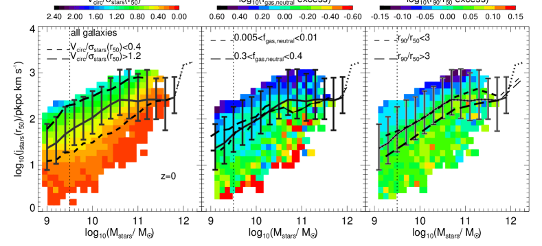
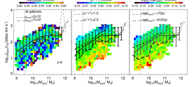
Figure 1: The specific angular momentum of the stars, measured with all the particles within $r_{50}$, as a function of stellar mass at $z=0$ for all galaxies with $M_{\rm stars}>10^{9}\,\rm M_{\odot}$. In each panel, the $j_{\rm stars}(r_{50})-M_{\rm stars}$ plane is colour coded according to the median $V_{\rm rot}(r_{50})/\sigma_{\rm stars}(r_{50})$ (top-left panel), neutral gas fraction (top-middle panel), $r_{\rm 50}/r_{90}$ (top-right panel), $\mu_{\rm stars}$ (measured within the inner $3$ pkpc; bottom-left panel), (u^∗-r^∗) colour (bottom-middle panel) and mass-weighted stellar age, $\langle\rm age_{\rm stars}\rangle$ (bottom-right panel), in pixels with $\geq 5$ objects. Here excess is defined as the ratio between the median in the 2-dimensional bin divided by the median at fixed stellar mass, so that negative (positive) values indicate galaxies to be below (above) the median at fixed stellar mass. In each panel the solid line and error bars indicate the median and $16^{\rm th}$ to $84^{\rm th}$ percentile range of $j_{\rm stars}(r_{50})$ at fixed stellar mass, while the short and long-dashed lines show two subsamples of galaxies (as labelled in each panel). Bins with $<10$ galaxies are shown as thinner lines. For reference, the vertical dotted line shows a conservative stellar mass limit above which $j_{\rm stars}$ is well converged for the resolution of the simulation.

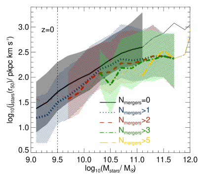
Figure 2: $j_{\rm stars}(r_{\rm 50})$ as a function of stellar mass, at $z=0$, for galaxies with $M_{\rm stars}>10^{9}\,\rm M_{\odot}$ in eagle. We show this relation for galaxies selected by the number of mergers they suffered throughout their history, as labelled. Lines show the median relations, while the shaded regions show the $16^{\rm th}-84^{\rm th}$ percentile range, but only for the cases of $N_{\rm mergers}=0,\,>1,\,>2,\,>3$. For reference, the vertical line shows a conservative stellar mass limit above which $j_{\rm stars}$ is well converged for the resolution of the simulation (see Appendix A for details). Note that here we only consider as galaxy mergers those with a baryonic mass ratio $\geq 0.1$. Mass ratios below that are considered to be below the resolution limit (Crain et al., 2016).

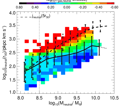
Figure 3: $j_{\rm neutral}$, measured within $r_{\rm 50}$, as a function of the neutral gas mass $z=0$ for galaxies with $M_{\rm stars}>10^{9}\,\rm M_{\odot}$. The solid line with error bars indicate the median and $16^{\rm th}$-$84^{\rm th}$ percentile range, respectively. Pixels with more than $5$ galaxies are coloured by the normalised median $f_{\rm gas,neutral}$, as indicated by the colour bar at the top. The dashed line with error bars show the median and $16^{\rm th}$-$84^{\rm th}$ percentile range, respectively, of the relation between $j_{\rm neutral}$, measured within $5\times r_{\rm 50}$, and the neutral gas mass.

The top left panel of Fig. 1 shows the correlation between $j_{\rm stars}(r_{50})$ and $M_{\rm stars}$ for galaxies with $M_{\rm stars}>10^{9}\,\rm M_{\odot}$ at $z=0$ in eagle. We find a moderately tight correlation between $j_{\rm stars}$ and $M_{\rm stars}$, with a scatter (i.e. standard deviation) of $\approx 0.6$ dex at fixed stellar mass. Galaxies with $10^{9}\,\rm M_{\odot}<M_{\rm stars}\lesssim 10^{10.6}\,\rm M_{\odot}$ display an increasing $j_{\rm stars}$ with increasing $M_{\rm stars}$, while for higher stellar mass galaxies, $j_{\rm stars}$ flattens. This is related to the transition from disk-dominated to bulge-dominated galaxies in eagle at $z=0$ (Zavala et al. 2016) and to the occurrence of galaxy mergers. The latter is shown in Fig. 2, which shows the $j_{\rm stars}-M_{\rm stars}$ relation for galaxies that have had no mergers, at least one merger, and successively up to at least $5$ mergers. We identified mergers using the merger trees available in the eagle database (McAlpine et al., 2015). Here we do not distinguish mergers that took place recently or far in the past, but just count their occurrence. At fixed stellar mass, galaxies with a higher incidence of mergers have significantly lower $j_{\rm stars}$. For example, at $M_{\rm stars}\approx 10^{10.7}\,\rm M_{\odot}$, galaxies that had never had a merger have $0.5$ dex higher $j_{\rm stars}$ than galaxies that suffered more than $5$ mergers in their lifetime. We present a comprehensive analysis of the effect of mergers on $j_{\rm stars}$ in an upcoming paper (Lagos et al. in preparation).

In eagle we find that several galaxy properties that trace morphology are related to $\lambda_{\rm R}$ and $j_{\rm stars}$ (Fig. 19), and thus the scatter of the $j_{\rm stars}-M_{\rm stars}$ relation is also expected to correlate with these properties. Indeed we find clear trends with all these properties in the middle and right panels of Fig. 1. To remove the trend between these properties and stellar mass, we coloured pixels by the median value of each property in each pixel divided by the median in the stellar mass bin. We name this ratio as excess. Galaxies with lower $f_{\rm gas,neutral}$, redder optical colours and higher stellar concentrations have lower $j_{\rm stars}$. We do not find a relation between the scatter in the $j_{\rm stars}-M_{\rm stars}$ relation with $\mu_{\rm stars}$ This is interesting, as recently Woo et al. (2015) suggested that $\mu_{\rm stars}$ is a good proxy of morphology. This is not seen in eagle as there is very little correlation between being rotationally- or dispersion-dominated and $\mu_{\rm stars}$. We cannot rule out at this point that the lack of correlation could be due to $\mu_{\rm stars}$ being measured here in apertures that are much larger than what observers use ($3$ vs. $1$ pkpc).

We find that the scatter of the $j_{\rm stars}-M_{\rm stars}$ relation is most strongly correlated with the $V_{\rm rot}/\sigma_{\rm stars}$ ratio and the gas fraction excess (top left and middle panels of Fig. 1). The trend with $V_{\rm rot}/\sigma_{\rm stars}$ is obtained almost by construction, given that $V_{\rm rot}\propto j_{\rm bar}$ and at $z=0$ $j_{\rm stars}\sim j_{\rm bar}$ due to the low gas fractions most galaxies have (note that the latter is not necessarily true for very gas-rich galaxies). Galaxies with $\rm log_{10}(f_{\rm gas,neutral}\,excess)<-0.5$ have $\approx 1.5$ dex lower $j_{\rm stars}$ than those with $\rm log_{10}(f_{\rm gas,neutral}\,excess)>0.3$, at fixed stellar mass. We do not find any differences between central and satellite galaxies, which is not necessarily surprising given that the angular momentum of the stars follows the angular momentum of the inner DM halo, rather than the total halo (Zavala et al., 2016), and thus it is less likely to be strongly affected by galaxies becoming satellites and any associated stripping of their outer halo.

We find that eagle galaxies with large values of $r_{90}/r_{50}$ have lower $j_{\rm stars}$ at fixed stellar mass (see for example the short- and long-dashed lines in the right panel of Fig. 1). If we instead measure $j_{\rm stars}$ out to $5$ times $r_{50}$, the relation between the scatter of the $j_{\rm stars}-M_{\rm stars}$ relation and $r_{90}/r_{50}$ mostly disappears (not shown here), indicating that this correlation arises only if we look at the central parts of galaxies. As for the intrinsic $\rm(u^{*}-r^{*})$ colour, we find that red galaxies, $\rm(u^{*}-r^{*})>2.2$, have $0.3$ dex lower $j_{\rm stars}$ than their bluer counterparts, $\rm(u^{*}-r^{*})<1.5$, at fixed stellar mass (bottom middle panel of Fig. 1). A similar difference is found between galaxies that have mass-weighted stellar ages $\rm\langle\rm age_{\rm stars}\rangle>9.5$ Gyr, and their younger counterparts with $\rm\langle\rm age_{\rm stars}\rangle<7$ Gyr, at fixed stellar mass.

A major conclusion that can be drawn from Fig. 1 is that eagle reproduces the observational trends of late-type galaxies having much larger $j_{\rm stars}$ than early-type galaxies (Fall, 1983; Romanowsky & Fall, 2012; Fall & Romanowsky, 2013). This is seen in most of the morphological indicators we use. In addition, Zavala et al. (2016) showed that this trend is also obtained in eagle using the distribution of circular orbits as a proxy for morphology. In Fig. 19 we show the correlation between the morphological indicators used here and the $\lambda_{\rm R}$ parameter, which is widely used in the literature to define slow and fast rotators.

Very similar correlations to those shown in Fig. 1 are find in the $j_{\rm bar}-M_{\rm bar}$ plane (shown in Fig. 21). The most important difference is that we do not find a strong correlation between the scatter in the $j_{\rm bar}-M_{\rm bar}$ relation and $r_{90}/r_{50}$.

Interestingly, in the $j_{\rm neutral}-M_{\rm neutral}$ relation, Fig. 3 shows that galaxies with high $f_{\rm gas,neutral}$ lie below the median. This trend remains when we study $j_{\rm neutral}$ out to larger radii. We interpret this trend as due to two factors: (i) as gas is consumed in star formation, galaxies move to the left of the diagram, and (ii) stars preferentially form from low-$j_{\rm neutral}$ gas, so by taking some of this low $j$ out, the $j_{\rm neutral}$ of the remaining gas increases, and hence galaxies also move up on the diagram.

4.1 Comparisons to observations

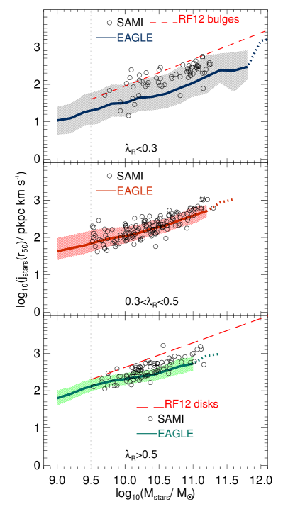
Figure 4: The $j_{\rm stars}(r_{\rm 50})-M_{\rm stars}$ relation at $z=0$ in three bins of $\lambda_{\rm R}$, as labelled in each panel. Lines and shaded regions show the median and $16^{\rm th}$ to $84^{\rm th}$ percentile ranges, respectively. Bins with less than $10$ objects are shown as dotted lines. Symbols show the observations of the SAMI survey (Cortese et al., 2016), and are shown in the different panels for the same bins of $\lambda_{\rm R}$ as adopted in eagle. We also show the observational result of Romanowsky & Fall (2012) (RF12) for bulges in the top panel (short-dashed line), and disks in the bottom panel (long-dashed line) (Fig. $14$ in Romanowsky & Fall 2012). For reference, the vertical dotted lines show a conservative stellar mass limit above which $j_{\rm stars}$ is well converged for the resolution of the simulation. We find a very good agreement with the measurements of SAMI.

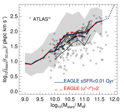
Figure 5: $j_{\rm stars}$ as a function of stellar mass for galaxies in eagle at $z=0$ with $M_{\rm stars}>10^{9}\,\rm M_{\odot}$ and with $\rm sSFR<0.01\,\rm Gyr^{-1}$ (solid line with shaded region) or with $\rm(u^{*}-r^{*})>2$ (dashed line). The selections in sSFR and $\rm(u^{*}-r^{*})$ colour are chosen to select passive objects in eagle  which is an effective way of selecting early-type galaxies. Here, $j_{\rm stars}$ in eagle is measured within the circularised half-mass radius, $r_{\rm 50,circ}$. The lines show medians and the shaded region show the median and $16^{\rm th}$ to $84^{\rm th}$ percentile range for the sSFR-selected sample. The scatter for the colour-selected sample is very similar and thus for clarity is not shown here. Circles show individual ATLAS^3D observations, while the long-dashed and thin solid lines show the median and the $16^{\rm th}$ to $84^{\rm th}$ percentile range of these observations in bins with $\geq 10$ galaxies.

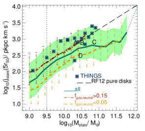
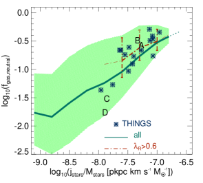
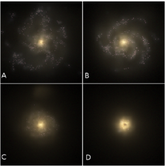
Figure 6: Left panel: $j_{\rm stars}$, measured within $5$ times the half-mass radius of the stellar component, as a function of stellar mass, for galaxies at $z=0$ with $M_{\rm stars}>10^{9}\,\rm M_{\odot}$ (no restriction in $\lambda_{\rm R}$ is applied here). The solid line and shaded region show the median and $16^{\rm th}$ to $84^{\rm th}$ percentile range, respectively. We also show the median and $16^{\rm th}$ to $84^{\rm th}$ percentile range of the relation for the subsample of galaxies with $f_{\rm gas,neutral}>0.15$ and $f_{\rm gas,neutral}<0.05$, as lines with error bars. Bins that with $<10$ objects are shown as dotted lines. Observational results from Obreschkow & Glazebrook (2014) using the THINGS survey are shown as star symbols. We also show the observational result of Romanowsky & Fall (2012) for disks. For reference, the vertical line shows a conservative stellar mass limit above which $j_{\rm stars}$ is well converged for the resolution of the simulation. Middle panel: As in the left panel, but here we show the neutral gas fraction, $f_{\rm gas,neutral}$, as a function of $j_{\rm stars}/M_{\rm stars}$. The relation for the subsample of galaxies with $\lambda_{\rm R}>0.6$ is shown as the dot-dashed line with error bars (median and $16^{\rm th}$ to $84^{\rm th}$ percentile range, respectively). Right panel: SDSS gri face-on images of $4$ eagle galaxies with $M_{\rm stars}=10^{10.3}-10.0^{10.7}\,\rm M_{\odot}$ and $f_{\rm gas,neutral}>0.15$ (top images) or $f_{\rm gas,neutral}<0.05$ (bottom images), constructed using the radiative transfer code SKIRT (Baes et al., 2011) (Trayford et al. in preparation). The images are $60\,\rm pkpc$ on a side and the positions of these galaxies, A, B, C and D, in the left and middle panels are shown with the corresponding. These images are publicly available from the eagle database (McAlpine et al., 2015). The figure shows that gas-rich galaxies have significantly higher $j_{\rm stars}$ and agree better with the THINGS observations. These galaxies appear visually to be similar to the late-type galaxies observed by THINGS.

Here we compare the predictions of eagle with four sets of observations: the Romanowsky & Fall (2012) sample, the ATLAS^3D survey (Cappellari et al., 2011a), the SAMI survey (Croom et al., 2012) and the THINGS survey (Walter et al., 2008; Obreschkow & Glazebrook, 2014). Below we give a brief overview of how $j_{\rm stars}$ was calculated in the four datasets used here.

• Romanowsky & Fall (2012). This corresponds to a sample of $\approx 100$ galaxies. Unlike the other observational samples we use here, measurements from Romanowsky & Fall (2012) were not done using resolved kinematic information, but instead they use long-slit spectroscopy and the HI emission line. This means that these measurements are considered to be total stellar specific angular momentum.

• ATLAS^3D. In order to calculate the stellar angular momentum within the effective (half-light) radius of the ATLAS^3D early-type galaxies (ETGs), we retrieved the stellar kinematics for all $260$ objects derived in Cappellari et al. (2011a). Following Obreschkow & Glazebrook (2014), we correct the projected velocity observed in each spaxel of the IFU for inclination by assuming a thin disc model for each object, with the position angle derived in Krajnović et al. (2011) and the inclination from Cappellari et al. (2013). Spaxels very close to the minor axis of the galaxy were blanked, to avoid numerical artefacts. From these de-projected velocities we calculate $j_{\rm stars}$ within the effective radius (taken from Cappellari et al. 2011a) following the equations in Obreschkow & Glazebrook (2014). We note that a thin disk model may not be appropriate for ETGs, which can have significant bulge components. As ATLAS^3D have shown that $\approx 86$% of these objects are fast rotators (Emsellem et al., 2011), with embedded stellar discs (Krajnović et al., 2013b, a) and axisymmetric rotation curves (Cappellari et al., 2011b), we do not expect this procedure to yield significant bias. In addition, Naab et al. (2014) showed that fast rotators in simulations have velocity moments that are consistent with disks. However, results for slow rotators should be treated carefully, as this approximation is likely to be inappropriate in that regime. Measurements in ATLAS^3D were done in circularised effective radii. The latter is $\approx 1.4$ times smaller than for example the ones used in SAMI (described below) at fixed stellar mass (and for the same morphological type). Thus, to compare eagle with ATLAS^3D we therefore need to produce a similar estimate of a circularised, 2-dimensional projected $r_{50}$ and then measure $j_{\rm stars}$ within that aperture. We call the latter radius $r_{\rm 50,circ}$.

• SAMI. Cortese et al. (2016) presented the measurements of the $j_{\rm stars}-M_{\rm stars}$ relation for galaxies of different morphological types and different values of $\lambda_{\rm R}$, in the stellar mass range $10^{9.5}\,\rm M_{\odot}\lesssim M_{\rm stars}\lesssim 10^{11.4}\,\rm M_{\odot}$. Cortese et al. measured $j_{\rm stars}$ within an effective radius from the line-of-sight velocity measured in each spaxel, and following the optical ellipticity and position angle of galaxies. These measurements are then corrected for inclination. Note that here the effective radius is similar to how we measure $r_{50}$ in eagle  and thus we can directly compare the results presented in $\S$ 4 with SAMI.

• THINGS. In the case of the THINGS survey, Obreschkow & Glazebrook (2014) presented a measurement of the $j_{\rm stars}$-stellar mass relation, where $j_{\rm stars}$ was measured within $\approx 10$ times the scale radius, which for an exponential disk, corresponds to $\approx 5$ times the half-mass radius. These represent the most accurate measurements of $j_{\rm stars}$ and $j_{\rm bar}$ to date, owing to the very high resolution and depth of the dataset used by Obreschkow & Glazebrook (2014). These measurements are not comparable to those of ATLAS^3D and SAMI, given that the latter only probe $j$ within $r_{\rm 50}$.

In Fig. 4 we present the $j_{\rm stars}(r_{50})$-stellar mass relation in three bins of $\lambda_{\rm R}$, $<0.3$, $0.3-0.5$ and $>0.5$. The predicted relations here are much tighter than the one shown in the top panel of Fig. 1, with a scatter of $\approx 0.15-0.3$ dex, which is a consequence of the limited range of $\lambda_{\rm R}$ studied in each panel.

The top panel of Fig. 1 shows galaxies with $\lambda_{\rm R}<0.3$ in both simulation and observations. SAMI galaxies are shown as symbols. eagle is in broad agreement with SAMI, although with a slightly smaller median than that of SAMI galaxies. The predicted $1\sigma$ dispersion in eagle is also similar to the one measured in SAMI, which is $\approx 0.26$ dex (Cortese et al., 2016). Here we also show the approximate location of the observational results of Romanowsky & Fall (2012) for bulges and found that they are on the upper envelope of both SAMI and eagle. This is not surprising given that Romanowsky & Fall (2012) presented measurements of the total $j_{\rm stars}$. In the middle panel of Fig. 4 we show galaxies with $0.3\leq\lambda_{\rm R}<0.5$. The observations of SAMI show that the increase in normalisation once higher $\lambda_{\rm R}$ galaxies are selected is very similar to the increase obtained in eagle. The bottom panel of Fig. 4 shows galaxies with $\lambda_{\rm R}\geq 0.5$. Here, SAMI galaxies lie slightly above the eagle galaxies at $M_{\rm stellar}\gtrsim 10^{10.7}\rm\,M_{\odot}$, although well within the $1\sigma$ dispersion in both samples. Also shown is the approximate location of the observational results of Romanowsky & Fall (2012) for disks. The slope of this sample is slightly steeper than what we obtain for eagle galaxies. The results of Fig. 4 are consistent with eagle and SAMI galaxies spanning a continuous sequence in the $j_{\rm stars}$-stellar mass plane, that go from low $j$-low $\lambda_{\rm R}$-low $V_{\rm rot}/\sigma_{\rm stars}$ to high $j$-high $\lambda_{\rm R}$-high $V_{\rm rot}/\sigma_{\rm stars}$.

To compare with ATLAS^3D we measure $j_{\rm stars}$ inside the circularised, 2-dimensional half-mass radius of the stellar component, $r_{\rm 50,circ}$. We do this by taking the projected stellar mass map on the $x-y$ plane and measuring the half-mass radius in circular apertures. In addition, we select galaxies in eagle that are passive, which would match well the properties of ATLAS^3D ETGs (mostly passive, except for a couple of galaxies). We use two selections: (1) eagle galaxies with a specific SFR (sSFR) $<0.01\,\rm Gyr^{-1}$, which would select galaxies below the main sequence in the $\rm SFR-M_{\rm stars}$ plane (Furlong et al. 2015a), and (2) eagle galaxies with $\rm(u^{*}-r^{*})>2$, which selects galaxies in the red sequence (Trayford et al. 2016). We compare the above subsamples with ATLAS^3D in Fig. 5. We find that both subsamples of eagle galaxies agree very well with the measurements, albeit with eagle possibly predicting a slightly shallower relation. However, the difference is well within the uncertainties. The scatter of eagle is slightly larger than that found in ATLAS^3D ($0.6$ vs. $0.4$ dex, respectively). This may be due to the lack of a true morphological selection of galaxies in eagle  which would require a visual inspection of the synthetic $gri$ images. In addition, there are some ATLAS^3D galaxies with very low $j_{\rm stars}$ measurements. These are the slow rotators, and it is likely that our estimates are systematically lower in these objects because our disc assumption is not valid in this regime.

In the left panel of Fig. 6 we show the $j_{\rm stars}-M_{\rm stars}$ relation with $j_{\rm stars}$ now measured within $5\,r_{5}$, for galaxies with $M_{\rm stars}>10^{9}\,\rm M_{\odot}$ at $z=0$ in eagle. Individual measurements from Obreschkow & Glazebrook (2014) are shown as symbols. Here we show again the approximate location of the observational results of Romanowsky & Fall (2012) for disks. The observations of Obreschkow & Glazebrook (2014) are well within the scatter of the relation of all eagle galaxies, but the median of the simulation is systematically offset by $\approx 0.2$ dex to lower values of $j_{\rm stars}$. At $M_{\rm stars}\gtrsim 10^{10.3}\rm\,M_{\odot}$, eagle galaxies systematically deviate from the observations of Obreschkow & Glazebrook (2014) and Romanowsky & Fall (2012). To reveal the cause of the offset, we divide the eagle sample into gas-rich ($f_{\rm gas,neutral}>0.15$) and gas-poor ($f_{\rm gas,neutral}<0.05$) galaxies, and present the median and scatter of those sample as dot-dashed and dashed lines with error bars, respectively. The subsample of galaxies with $f_{\rm gas,neutral}>0.15$ shows no flattening of the $j_{\rm stars}-M_{\rm stars}$ relation and the median is shifted upwards to higher $j_{\rm stars}$. The sample of Obreschkow & Glazebrook (2014) is characterised by a median $f_{\rm gas,neutral}\approx 0.22$, meaning that it should be compared to the eagle sample with $f_{\rm gas,neutral}>0.15$. By doing this, we find excellent agreement between eagle and the THINGS observations. Thus, the $j_{\rm stars}-M_{\rm stars}$ relation found by Obreschkow & Glazebrook (2014) is not representative of the overall galaxy population at fixed stellar mass, but only of the relatively gas-rich galaxies.

To help visualise how gas-rich vs. gas-poor galaxies of the same stellar mass look like, we show SDSS gri face-on images of four eagle galaxies with stellar masses in the range $10^{10.3}-10^{10.7}\,\rm M_{\odot}$, and $f_{\rm gas,neutral}>0.15$ (galaxies A and B, top images) or $f_{\rm gas,neutral}<0.05$ (galaxies C and D, bottom images). These images were created using radiative transfer simulations performed with the code SKIRT (Baes et al., 2011) in the SDSS g, r and i filters (Doi et al., 2010). Dust extinction was implemented using the metal distribution of galaxies in the simulation, and assuming $40$% of the metal mass is locked up in dust grains (Dwek, 1998). The images were produced using particles in spherical apertures of $30$ pkpc around the centres of sub-halos (see Trayford et al. 2015, and in preparation for more details). It is clear that galaxies that look like regular spiral galaxies in eagle correspond to those having $f_{\rm gas,neutral}\gtrsim 0.15$, while gas-poor galaxies look like lenticulars or early-type galaxies. Galaxies C and D have $\lambda_{\rm R}(r_{\rm 50})\approx 0.45$, which would be classified observationally as fast rotators early-type galaxies in the nomenclature of the ATLAS^3D survey (Cappellari et al., 2011a). The positions of these galaxies in the $j_{\rm stars}$-$M_{\rm stars}$ plane are shown in the left and middle panel of Fig. 6 with the corresponding letters. We visually inspected $100$ galaxies randomly selected ($50$ in the gas-rich and $50$ in the gas poor subsamples), and found the differences presented here (between galaxies A-B and C-D) to be generic.

We further characterise the relation between $j_{\rm stars}$, stellar mass and $f_{\rm gas,neutral}$ in the middle panel of Fig. 6, that shows $f_{\rm gas,neutral}$ vs. $j_{\rm stars}/M_{\rm stars}$ for eagle galaxies at $z=0$ with $M_{\rm stars}>10^{9.5}\,\rm M_{\odot}$. In eagle galaxies that are more gas rich, also have a higher $j_{\rm stars}/M_{\rm stars}$. The scatter is slightly reduced if we select galaxies in narrow ranges of $\lambda_{\rm R}$ (see dot-dashed line with error bars in the middle panel of Fig. 6). The observations of Obreschkow & Glazebrook (2014) fall within the $1\sigma$ scatter of the relation in eagle, which shows that the simulation captures how the angular momentum together with the gas content of galaxies are acquired.

The agreement between the simulation and the observations is quite remarkable. eagle not only reproduces the normalisation of the $j_{\rm stars}$-stellar mass relation, which may not be so surprising given that eagle matches the size-stellar mass relation well (Schaye et al., 2015; Furlong et al., 2015a), but also the trends with $\lambda_{\rm R}$ and $f_{\rm gas,neutral}$ as identified by observations.

5 The evolution of the specific angular momentum of galaxies in eagle

Here we analyse the evolution of $j_{\rm stars}$ and $j_{\rm neutral}$ as a function of galaxy properties and attempt to find those properties that are more fundamentally correlated to them.

5.1 The evolution of the $j$-mass relations

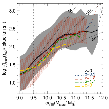
Figure 7: The specific angular momentum of the stars measured with all the particles within the half-mass radius of the stellar component as a function of stellar mass at $z=0$, $0.5$, $1.2$, $1.7$ and $3$, as labelled, for all galaxies with $M_{\rm stars}>10^{9}\,\rm M_{\odot}$ and $r_{rm50}>1$ pkpc in eagle. Lines show the median relations, while the shaded regions show the $16^{\rm th}$ to $84^{\rm th}$ percentile ranges, and are only shown for $z=0,\,1.2$. For reference, the vertical dotted line shows a conservative stellar mass limit above which $j_{\rm stars}$ is well converged for the resolution of the simulation, and the straight solid lines show the scalings $j\propto M$, $j\propto M^{2/3}$ and $j\propto M^{1/3}$, as labelled.

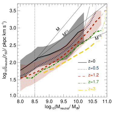
Figure 8: As in Fig. 7, but here we show $j_{\rm neutral}$ as a function of neutral gas mass. At fixed mass, galaxies at high redshift have lower $j_{\rm neutral}$ than the $z=0$ counterparts.

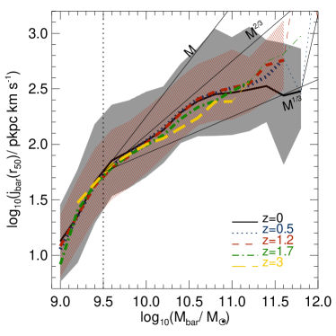
Figure 9: As in Fig. 7, but here we show $j_{\rm bar}$ as a function of baryon mass (stars plus neutral gas).

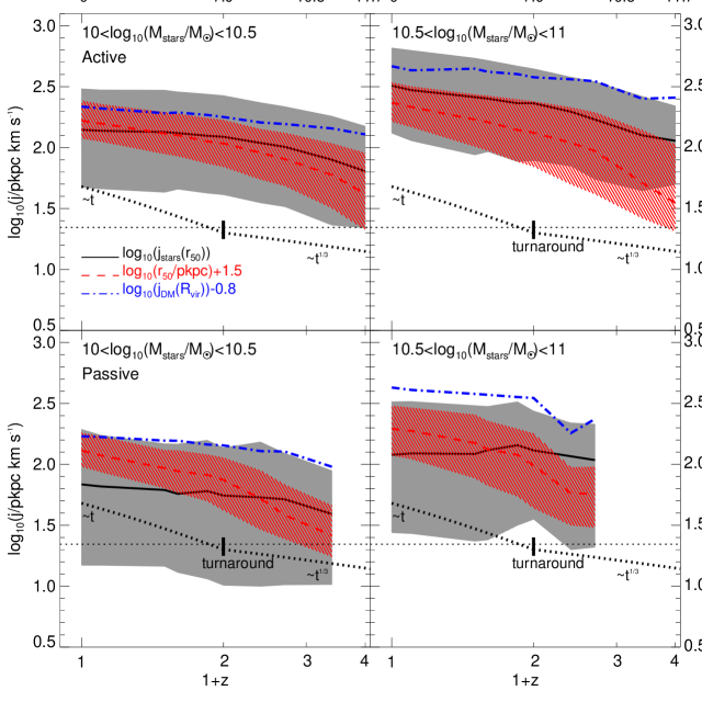
Figure 10: Evolution of $j_{\rm stars}(r_{50})$ for central galaxies in eagle in two bins of stellar mass, as labelled in each panel, and separated into active (top panels) and passive (bottom panels) galaxies. The latter classification is made based on their position with respect to the main sequence. Look-back time is shown at the top. The line and shaded region shows the median and $16^{\rm th}-84^{\rm th}$ percentile range of $j_{\rm stars}(r_{50})$, respectively. Only bins with $\geq 10$ galaxies are shown. The $j$ of the host DM halo, $j_{\rm DM}(\rm R_{\rm vir})$ (scaled by $-0.8$ dex) is shown as dot-dashed lines. We also show the evolution of half-mass radius of the stellar component, $r_{50}$, plus $1.5$ dex to match the normalisation of $j_{\rm stars}$ (median and $16^{\rm th}-84^{\rm th}$ percentile range shown as dashed line with shaded region, respectively). In each panel we show for reference the maximum gravitational softening length of the simulation (plus $1.5$ dex) as horizontal dotted line (at $z\geq 2.7$ it decreases as $(1+z)$, but for clarity we do not show that here). The vertical segments show roughly the turnaround epoch of the host halos. In addition, we show as dotted line (using an arbitrary normalisation) the prediction of Catelan & Theuns (1996a) of how $j_{\rm stars}$ grows with time before and after the turnaround epoch. The latter is only for reference, and should not be taken as a test of the theoretical predictions, given that here we are not tracing galaxy progenitors, but instead selecting similar galaxy populations at different redshifts. This figure shows that galaxy sizes evolve much more strongly than $j_{\rm stars}$ at fixed stellar mass, and that star-forming galaxies exhibit a stronger increase in $j_{\rm stars}$ than passive galaxies.

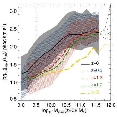
Figure 11: The specific angular momentum of the stars measured at different redshifts as a function of the stellar mass galaxies have at $z=0$. In the case of $j$, we measure it at $z=0$, $0.5$, $1.2$, $1.7$ and $3$, as labelled, with all the particles within the half-mass radius of the stellar component at the redshift. We show the relation for all galaxies with $M_{\rm stars}>10^{9}\,\rm M_{\odot}$ at $z=0$ in eagle. Lines show the median relations, while the shaded regions show the $16^{\rm th}$ to $84^{\rm th}$ percentile ranges, and are only shown for $z=0,\,0.5,\,1.2$. Bins with $<10$ objects are shown as thin lines. This figure shows that progenitor galaxies typically have lower $j$ than their descendants. For reference, the vertical line shows a conservative stellar mass limit above which $j_{\rm stars}$ is well converged for the resolution of the simulation.

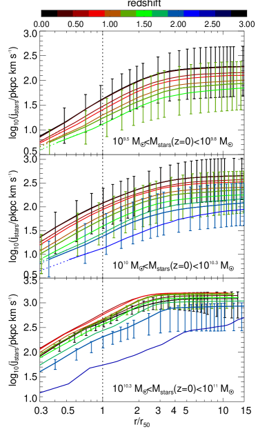
Figure 12: $j_{\rm stars}$ measured within $r$ as a function of $r$ in units of $r_{\rm 50}$ at different redshifts, as shown by the color bar, for galaxies with $z=0$ stellar mass in three bins, as labelled in each panel. Solid lines show the median, while the error bars show the $16^{\rm th}$ to $84^{\rm th}$ percentile ranges. The latter are only shown for $z=0,\,1,\,1.7$. Dotted lines show the extrapolation of the profiles towards radii that are below $1$ pkpc (approximately the spatial resolution of eagle). The vertical dotted lines shows $r=r_{\rm 50}$. The range span by the y-axis changes in each panel to better cover the dynamic range of $j_{\rm stars}$ in each stellar mass bin. This figure shows that $j_{\rm stars}(r_{\rm 50})$ evolves more strongly than $j_{\rm stars}$ measured at larger apertures.

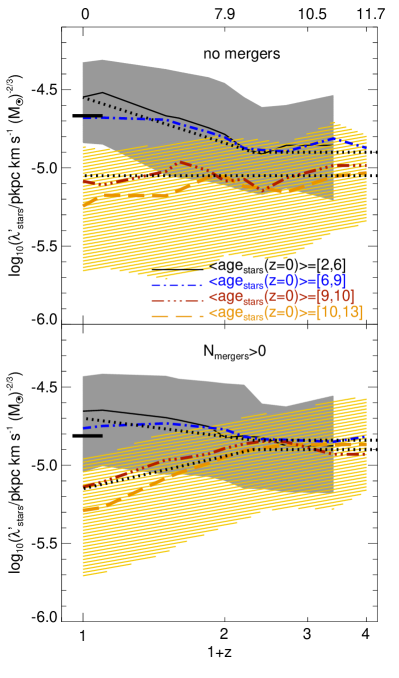
Figure 13: The value of $\lambda^{\prime}_{\rm stars}\equiv j_{\rm stars}(r_{50})/M^{2/3}_{\rm stars}$ as a function of redshift, for eagle galaxies selected in different bins of mass-weighted stellar age at $z=0$, $\langle\rm age_{\rm stars}\rangle$, as labelled (with numbers in the figure being in Gyr), and that have $M_{\rm stars}(z=0)\geq 10^{9.5}\,\rm M_{\odot}$. Look-back time is shown at the top. Lines show the median relations, and the shaded regions show the $25^{\rm th}$ to $75^{\rm th}$ percentile ranges, and for clarity we only show this for the lowest and highest $\rm\langle\rm age_{\rm stars}\rangle$ bins. In the top panel we show the subsamples of galaxies at $z=0$ that had not suffered galaxy mergers, while the bottom panel shows the complement. The segment in both panels show the median of the selected galaxy population at $z=0$, while the dotted lines show the average evolutionary tracks of Table 2.

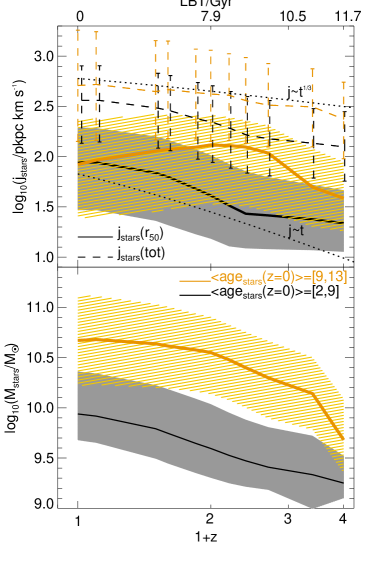
Figure 14: Top panel: Evolution of the median $j_{\rm stars}(r_{50})$ (solid lines) and $j_{\rm stars}(\rm tot)$ (dashed lines) for two samples of galaxies selected by their mass-weighted stellar age at $z=0$, as labelled in the bottom panel. $j_{\rm stars}(\rm tot)$ is measured with all the star particles in the sub-halo, while $j_{\rm stars}(r_{50})$ only with those within $r_{\rm 50}$. Lines show the medians, while the shaded regions and error bars show the $25^{\rm th}$ to $75^{\rm th}$ percentile ranges. The dotted lines (using an arbitrary normalisation) show the prediction of Catelan & Theuns (1996a, b) of how $j$ grows with time before the turnaround epoch ($j\propto t^{1/3}$), and the upper limit for the time dependence of the specific angular momentum of infalling material after turnaround ($j\propto t$). The latter could therefore be considered as an upper limit for how fast $j_{\rm stars}(\rm tot)$ can increase. Bottom panel: Evolution of the median stellar mass of the galaxies shown in the top panel. This figure shows that galaxies throughout their lifetimes go through a significant rearrangement of their $j_{\rm stars}$ in a way that young galaxies have inner $j_{\rm stars}$ growing faster than the total value, while old galaxies at $z\lesssim 1$, have inner $j_{\rm stars}$ decreasing, while their total $j_{\rm stars}$ shows little evolution.

Fig. 7 shows the $j_{\rm stars}(r_{\rm 50})-M_{\rm stars}$ relation in the redshift range $0\leq z\leq 3$ for galaxies with $M_{\rm stars}>10^{9}\,\rm M_{\odot}$ and $r_{\rm 50}>1$ pkpc in eagle. Galaxies have lower $j_{\rm stars}(r_{\rm 50})$ at fixed stellar mass at high redshift. Interestingly, between $0\lesssim z\lesssim 0.5$ the normalisation of the $j_{\rm stars}(r_{\rm 50})-M_{\rm stars}$ relation evolves weakly. The strongest change experienced by galaxies is at $1\leq z\leq 3$ (of $\approx 0.2-0.35$ dex). The stellar mass above which the $j_{\rm stars}(r_{\rm 50})-M_{\rm stars}$ relation flattens has a small tendency of increasing with decreasing redshift. At $z\approx 1.2$ the flattening is seen above $\approx 10^{10.3}\,\rm M_{\odot}$, while at $z=0$ the flattening starts at $10^{10.5}\,\rm M_{\odot}$. There are no available observational measurements of $j_{\rm stars}(r_{\rm 50})$ at high redshift yet, but there are measurements of how the effective radius and the rotational velocity of galaxies evolve. van der Wel et al. (2014) showed that galaxies at fixed stellar mass are $\approx 1.9$ times smaller at $z=1$ compared to $z=0$, while in the same redshift range Tiley et al. (2016) showed that galaxies increase their rotational velocity by $\approx 1.3$. If one assumes that $j_{\rm stars}\sim r_{50}\,V_{\rm rot}$, then these observations imply a decrease of $j_{\rm stars}$ at fixed stellar mass from $z=0$ to $z=1$ of $\approx 1.4-1.5$, very similar to the magnitude of evolution in $j_{\rm stars}$ we obtain from eagle at $0\leq z\leq 1.2$.

The flattening of the $j_{\rm stars}(r_{\rm 50})-M_{\rm stars}$ relation at high stellar masses is mostly driven by galaxy mergers (Fig. 2). In Fig. 7 we also show for comparison the scalings $j\propto M$, $j\propto M^{2/3}$ and $j\propto M^{1/3}$. A scaling $j\propto M$ is expected in the model of Obreschkow & Glazebrook (2014), where galaxies are well described by the relation $Q\propto j_{\rm stars}\,M^{-1}_{\rm stars}\,(1-f_{\rm gas,neutral})\,\sigma$, while a relation $j\propto M^{2/3}$ is predicted in a CDM universe under the assumption of conservation of $j$ ($\S$ 3). Galaxies with stellar masses below the flattening and at $z\lesssim 1$ follow a scaling close to $j_{\rm stars}\propto M^{2/3}_{\rm stars}$, while at higher redshifts the relation becomes steeper, which is most evident in the mass range $10^{9.4}\,\rm M_{\odot}\lesssim M_{\rm stars}\lesssim 10^{10.5}\,\rm M_{\odot}$. By fitting the $j_{\rm stars}(r_{\rm 50})-M_{\rm stars}$ relation using a power-law and the HYPER-FIT R package of Robotham & Obreschkow (2015) we find that the best fit power-law index at $z\gtrsim 1$ in the stellar mass range above is $\approx 0.77$.

Fig. 8 shows the $j_{\rm neutral}(r_{\rm 50})-M_{\rm neutral}$ relation for galaxies with $M_{\rm stars}>10^{9}\,\rm M_{\odot}$ and $r_{\rm 50}>1$ pkpc at $0\leq z\leq 3$ in eagle. Galaxies evolve significantly in this plane, having $\approx 3-5$ times lower $j_{\rm neutral}$ at $z\approx 3$ than they do at $z=0$ at fixed $M_{\rm neutral}$. By fitting the $j_{\rm neutral}-M_{\rm neutral}$ relation using HYPER-FIT we find that the best fit power-law index is $\approx 0.5-0.6$, with the exact value depending on the redshift. Thus, on average, this relation is close to the theoretical expectation of $j\propto M^{2/3}$.

In Fig. 9 we show the $j_{\rm bar}(r_{\rm 50})-M_{\rm bar}$ relation for galaxies with $M_{\rm bar}>10^{9}\,\rm M_{\odot}$ and $r_{\rm 50}>1$ pkpc at $0\leq z\leq 3$ in eagle. There is little evolution of the $j_{\rm bar}-M_{\rm bar}$ at $M_{\rm bar}\lesssim 10^{10}\,\rm M_{\odot}$. Galaxies with $10^{10}\,\rm M_{\odot}\lesssim M_{\rm bar}\lesssim 10^{11}\,\rm M_{\odot}$, display a modest evolution of $j_{\rm bar}$ at $1\lesssim z\lesssim 3$ of $\approx 0.2$ dex, with little evolution below $z\sim 1$. Galaxies with $M_{\rm bar}\gtrsim 10^{11}\,\rm M_{\odot}$ have $j_{\rm bar}(r_{\rm 50})$ decreasing at fixed stellar mass. The latter is due to galaxies becoming increasingly gas poor, and thus going from $j_{\rm bar}$ being dominated by $j_{\rm neutral}$ to being dominated by $j_{\rm stars}$. The former is almost always higher than the latter. Note that the power-law index of the $j_{\rm bar}$-baryon mass does not change significantly with redshift and is always close to $\approx 0.6$, although noticeable differences are seen with stellar mass, at fixed redshift.

5.1.1 $j_{\rm stars}$ evolution in active and passive galaxies

Fig. 10 shows the evolution of $j_{\rm stars}(r_{\rm 50})$ for active and passive central galaxies in two bins of stellar mass. We select central galaxies to enable us to compare with $j_{\rm DM}(\rm R_{\rm vir})$, which is calculated with all DM particles within the virial radius of the friends-of-friends host halo. For comparison, we also show the evolution of $r_{50}$. We separate galaxies into active and passive by calculating the position of the main sequence at each redshift, and then computing the distance in terms of sSFR to the main sequence, $\rm sSFR/\langle sSFR_{\rm MS}\rangle$. Galaxies with $\rm sSFR/\langle sSFR_{\rm MS}\rangle<0.1$ are considered passive, while the complement are active. The position of the main sequence, $\rm\langle sSFR_{\rm MS}\rangle$, is calculated as the median sSFR of all galaxies at a given redshift that have $\rm sSFR>sSFR_{\rm lim}$, where $\rm sSFR_{\rm lim}$ is defined as $\rm log_{10}(sSFR_{\rm lim}/Gyr^{-1})=0.5\,z-2$ for $z\leq 2$ and $\rm log_{10}(sSFR_{\rm lim}/Gyr^{-1})=-1$ for $z>2$ (see Furlong et al. 2015b for details).

Once the stellar mass is fixed, $j_{\rm stars}(r_{\rm 50})$ evolves very weakly in passive galaxies ($\approx 0.2$ dex between $0\leq z\leq 3$) and slightly more strongly in star-forming galaxies ($\approx 0.3-0.4$ dex between $0\leq z\leq 3$). We show the evolution of $j_{\rm DM}(R_{\rm vir})$ of the halo hosting the galaxies shown in Fig. 10, to stress the fact that the evolution of $j_{\rm stars}\sim j_{\rm DM}$, to within $\approx 50$% (i.e. the $1\sigma$ scatter around the constant of proportionality is $\approx 0.18$ dex). We remind the reader that we are not studying the evolution of individual galaxies here, but instead how $j$ evolves at fixed stellar mass and star formation activity, as defined by the distance of galaxies to the main sequence of star formation. The selection of galaxies in Fig. 10 roughly corresponds to halos of the same mass at different redshifts. At fixed mass, halos also show a slight increase in $j_{\rm DM}$ with time due to halos at lower redshift crossing turnaround at increasingly later times, which imply that they had longer times to acquire angular momentum. The similarity seen between $j_{\rm stars}(r_{50})$ and $j_{\rm DM}(\rm R_{\rm vir})$ means that to zeroth order any gastrophysics is secondary when it comes to the value of $j_{\rm stars}$ in galaxies, showing how fundamental this quantity is. However, when studied in detail, we find that galaxies undergo a significant rearrangement of their $j_{\rm stars}$ radial profile that is a result of galaxy formation. This rearrangement is also the cause of $j_{\rm DM}$ evolving much more weakly than $j_{\rm stars}(r_{\rm 50})$, particularly in star-forming galaxies. We come back to this in $\S$ 5.2.

The evolution of $j_{\rm stars}(r_{\rm 50})$ at fixed stellar mass in eagle mostly occurs at $z\gtrsim 1$, before the turnaround epoch of the halos hosting the galaxies of the stellar mass we are studying here, at $z=0$, which is $z\approx 1$. This epoch corresponds to the time of maximum expansion that is followed by the collapse of halos, after which $j_{\rm DM}$ is expected to be conserved (Catelan & Theuns, 1996a). Before turnaround halos continue to acquire angular momentum as they grow in mass. Turnaround epochs of the $z=0$ host halos are shown in Fig. 10 as vertical segments. On the other hand, the half-mass radius of the stellar component grows by $\gtrsim 0.7-0.9$ dex over the same period of time and at fixed stellar mass. This is interesting since in Fig. 10 we focus on $j$ measured within $r_{\rm 50}$, which implies that the radial profiles of $j_{\rm stars}$ in galaxies grow inside out. By studying the cumulative radial profiles of $j_{\rm stars}$ of the galaxies in Fig. 10 we find that typically galaxies have profiles becoming steeper with decreasing redshift, and that at $z\gtrsim 1$ the inner regions of galaxies evolve very weakly, while the outer regions display a fast increase of $j_{\rm stars}$ (not shown here). These trends result in $j_{\rm stars}(r_{\rm 50})$ not evolving or only slightly increasing (in the case of star-forming galaxies) at $z<1$, even though $j_{\rm stars}(r)$, with $r\lesssim 6$ pkpc, decreases in the same period of time. The former is therefore a consequence of $r_{\rm 50}$ rapidly increasing with time.

Catelan & Theuns (1996a) predicted from linear tidal torque theory in a CDM universe that a halo collapsing at turnaround has an angular momentum of $L\propto M^{5/3}\,t^{1/3}$, where the time dependence comes from how the collapse time depends on halo mass, and thus at fixed halo mass, $j_{\rm halo}\propto M^{2/3}\,t^{1/3}$ at the moment of collapse. Catelan & Theuns (1996a) also showed that in an Einstein de Sitter universe, the angular momentum of material falling into halos has $L\propto t$, which means that material falling later brings higher $L$. Under $j$ conservation, one could assume that $j_{\rm stars}$ follows a similar behaviour. We show in Fig. 10, using an arbitrary normalisation, how these time scalings compare with the evolution of eagle galaxies. $j_{\rm stars}(r_{\rm 50})$ closely follows the scaling of $t^{1/3}$ before the turnaround epoch while after turnaround $j_{\rm stars}(r_{\rm 50})$ is mostly flat (except for massive star-forming galaxies, that continue to display $j_{\rm stars}(r_{\rm 50})$ increasing), while $j_{\rm neutral}(r_{\rm 50})$ evolves close to $\propto t$. The latter is expected if the neutral gas is being freshly supplied by gas that is falling into halos. The comparison with the expected time scalings of Catelan & Theuns (1996a) should be taken as reference only, given that here we are not tracing the progenitors of galaxies, and thus the evolution seen in Fig. 10 does not correspond to individual galaxies. In $\S$ 5.2 we study how $j_{\rm stars}$ developed in individual galaxies, selected at $z=0$.

5.2 Tracing the development of $j$ in individual galaxies

Until now we have studied the evolution of $j$ at fixed mass throughout time, but mass is also a dynamic property, and thus in the $j$-$M$ plane both quantities are evolving in time. To quantify how much $j$ changes in a given galaxy, we look at all galaxies with $M_{\rm stars}>10^{9}\,\rm M_{\odot}$ at $z=0$ and trace back their progenitors. By doing so we keep the mass axis fixed (at $z=0$). We show in Fig. 11 the growth of $j_{\rm stars}$ at fixed $M_{\rm stars}$ at $z=0$. $j_{\rm stars}$ is measured within $r_{\rm 50}$ at different redshifts. Galaxies with stellar masses $<10^{10}\,\rm M_{\odot}$ at $z=0$ gain most of their $z=0$ $j_{\rm stars}(r_{\rm 50})$ at $z<1$. Between $10^{10}\,\rm M_{\odot}<M_{\rm stars}<10^{10.7}\,\rm M_{\odot}$ there is a transition, in a way that galaxies with $M_{\rm stars}>10^{10.7}\,\rm M_{\odot}$ at $z=0$ show the opposite behaviour, with most of their $j_{\rm stars}$ having been acquired at $z\gtrsim 1$. The latter display a rapid growth of $j_{\rm stars}$ at $1.2<z<3$ of $\approx 0.3-0.5$ dex, followed by a much slower growth at $0.5<z<1.2$ of $\approx 0.15$ dex. At $z<0.5$ these massive galaxies have $j_{\rm stars}(r_{\rm 50})$ even decreasing, due to the incidence of dry mergers (those with $f_{\rm gas,neutral}\lesssim 0.1$; Lagos et al. in preparation). Galaxies with stellar masses at $z=0$ in the range $10^{10.1}-10^{10.7}\,\rm M_{\odot}$ are the ones experiencing the largest increase in $j_{\rm stars}$ (Fig. 11). These galaxies grow their $j_{\rm stars}$ by $\approx 0.7-1$ dex from $\approx 3$ to $z=0$. We find that $j_{\rm bar}(r_{50})$ evolves very similarly to what is shown in Fig. 11.

Fig. 12 shows the evolution of the cumulative profiles of $j_{\rm stars}$ for galaxies selected by their $z=0$ stellar mass, in the redshift range $0\leq z\leq 3$. We find that $j_{\rm stars}$ in the inner regions of galaxies evolves faster than in the outer regions. This is particularly dramatic at the highest stellar mass bin shown in Fig. 12, where the total $j_{\rm stars}$ (measured with all the star particles of the sub-halo) increases by $\approx 0.5$ dex from $z\approx 3$ to $z\approx 0.8$, followed by a decline of $\approx 0.1$ down to $z=0$, while within $r_{50}$, $j_{\rm stars}$ increases by $\approx 1$ dex from $z\approx 3$ to $z\approx 0.8$, followed by a decrease of $\approx 0.2$ dex down to $z=0$. In the smallest mass bin the effect is subtle and there is only $\approx 0.1$ dex difference between the evolution of $j_{\rm stars}(r_{50})$ and $j_{\rm stars}(\rm tot)$ at $0\leq z\leq 3$, while at $z\lesssim 0.8$ the inner $j_{\rm stars}$ increases faster than the total $j_{\rm stars}$ by a factor of $\approx 1.4$. The latter effect is even stronger when young galaxies are considered (Fig. 14). We will come back to this point in $\S$ 5.2.1. The effect described here is partially due to $r_{50}$ increasing with time, which causes $j_{\rm stars}(r_{50})$ to also increase, but also due to an evolution in how $j_{\rm stars}$ is radially distributed in galaxies.

eagle shows that in addition to the total $j_{\rm stars}$ of galaxies evolving, they also suffer from significant radial rearrangement of their $j_{\rm stars}$ throughout their lifetimes.

5.2.1 Evolutionary tracks of $j/M^{2/3}$

Table 2: Average evolutionary tracks of $\lambda^{\prime}_{\rm stars}\equiv j_{\rm stars}(r_{50})/M^{2/3}_{\rm stars}$ for galaxies that never had a merger, or those that have had at least $1$ merger, and divided into galaxies with mass-weighted stellar ages $>$ or $<$ $9$ Gyr. The units of $\lambda^{\prime}_{\rm stars}$ are $\rm pkpc\,km\,s^{-1}$. These evolutionary tracks are shown as dotted lines in Fig. 13. We also show in parenthesis the percentage of $z=0$ galaxies with $M_{\rm stars}(z=0)\geq 10^{9.5}\,\rm M_{\odot}$ and $r_{50}(z=0)>1$ pkpc in eagle that roughly follow each evolutionary path.

	No mergers
$\langle\rm age_{\rm stars}\rangle\geq 9\,Gyr$	$\lambda^{\prime}_{\rm stars}=10^{-4.9}$
($\approx 2$%)
$\langle\rm age_{\rm stars}\rangle<9\,Gyr$	$\lambda^{\prime}_{\rm stars}=10^{-4.9},\,\,\,\,\,\,\,$ if $z\geq 1.2$
($\approx 10$%)	$\,\,\,\,\,\,\,\,\,\,\,\,\,\,\,\,\,\,\,\,\,\,\,10^{-4.55}\,a,$ if $z<1.2$
	$N_{\rm mergers}>0$
$\langle\rm age_{\rm stars}\rangle\geq 9\,Gyr$	$\lambda^{\prime}_{\rm stars}=10^{-4.9},\,\,\,\,\,\,\,\,\,\,\,\,\,\,\,\,\,$ if $z\geq 1.2$
($\approx 47$%)	$\,\,\,\,\,\,\,\,\,\,\,\,\,\,\,\,\,\,\,\,\,\,\,10^{-5.15}a^{-0.7},$ if $z<1.2$
$\langle\rm age_{\rm stars}\rangle<9\,Gyr$	$\lambda^{\prime}_{\rm stars}=10^{-4.85},\,\,\,\,\,\,\,\,\,$ if $z\geq 1.2$
($\approx 41$%)	$\,\,\,\,\,\,\,\,\,\,\,\,\,\,\,\,\,\,\,\,\,\,\,10^{-4.7}a^{0.4},$ if $z<1.2$

There are two dominant effects that determine the value of $j_{\rm stars}$ at any one time in a galaxy’s history: (i) whether stars formed before turnaround or after; those formed before tend to have lower $j_{\rm stars}$ than those formed after, and (ii) whether galaxies have undergone dry galaxy mergers; these systematically lower $j_{\rm stars}$ in galaxies. We define the spin parameter of the stars, $\lambda^{\prime}_{\rm stars}\equiv j_{\rm stars}(r_{50})/M^{2/3}_{\rm stars}$ (as on average $j_{\rm stars}(r_{50})\propto M^{2/3}_{\rm stars}$ in eagle), and show the evolution of $\lambda^{\prime}_{\rm stars}$ for galaxies that have different mass-weighted stellar ages at $z=0$ in Fig. 13. We name this parameter as $\lambda^{\prime}_{\rm stars}$ to distinguish it from the dimensionless spin parameter, defined in $\S$ 3. We separate galaxies that never suffered a galaxy merger (top panel) from those that went through at least one galaxy merger (bottom panel). Here galaxy mergers are defined as those with a mass ratio $\geq 0.1$, while lower mass ratios are considered to be accretion (Crain et al., 2016).

The top panel of Fig. 13 shows that galaxies with $\rm\langle\rm age_{\rm stars}\rangle\gtrsim 9\,Gyr$ have roughly constant $\lambda^{\prime}_{\rm stars}$ over time, albeit with large scatter. Most of the stars in these galaxies were formed before the epoch of turnaround. On the other hand, galaxies with $\rm\langle\rm age_{\rm stars}\rangle\lesssim 9\,Gyr$ show a significant increase in their $\lambda^{\prime}_{\rm stars}$ at $z\lesssim 1.2$, after turnaround. The extent to which the latter galaxies increase their $\lambda^{\prime}_{\rm stars}$ is very similar, despite the wide spread in ages.

In the subsample of galaxies that had at least one galaxy merger during their formation history (bottom panel of Fig. 13), the effects of mergers are apparent. Galaxies with $\rm\langle\rm age_{\rm stars}\rangle\gtrsim 9\,Gyr$ show a significant reduction of their $\lambda^{\prime}_{\rm stars}$ at $z\lesssim 1.2$ where most of the mergers are dry. Galaxies with $\rm\langle\rm age_{\rm stars}\rangle\lesssim 9\,Gyr$ that had mergers still show an increase of their $\lambda^{\prime}_{\rm stars}$ at $z\lesssim 1.2$ but to a lesser degree than the sample without mergers.

From Fig. 13, we extract average evolutionary tracks of $\lambda^{\prime}_{\rm stars}$. These are presented in Table 2, along with the percentage of $z=0$ galaxies that followed each evolutionary path, and are shown as dotted lines in Fig. 13. A powerful conclusion of Fig. 13 and Table 2 is that galaxies can have low $j_{\rm stars}$ either by the effects of mergers or by simply having formed most of their stars early on. The simple picture from Fall (1983) invoked only mergers to explain the low $j_{\rm stars}$ of early-type galaxies. Here we find a more varied scenario. The latter statement holds regardless of the aperture used to measure $j_{\rm stars}$, however, the exact evolutionary tracks obtained are sensitive to the aperture used, as we describe below.

Fig. 20 shows examples of these average tracks compare to the evolution of $\lambda^{\prime}_{\rm stars}$ in galaxies selected in bins of their host halo mass, and show that the they describe their evolution relatively well and that the variations with halo mass are mild.

The tracks we identified in eagle are partially driven by $j_{\rm stars}(r_{50})$ evolving more dramatically than the total $j_{\rm stars}$ in galaxies. This is shown in Fig. 14 where the evolution of $j_{\rm stars}(r_{50})$, $j_{\rm stars}\rm(tot)$ and $M_{\rm stars}$ are shown for galaxies in two bins of $\rm\langle\rm age_{\rm stars}\rangle$. The selection in $\rm\langle\rm age_{\rm stars}\rangle$ yields to two clear bins in stellar mass, which is due to the positive relation between $\rm\langle\rm age_{\rm stars}\rangle$ and stellar mass. In the case of old, massive galaxies, we find that before turnaround ($z\approx 1.2$ for these galaxies) $j_{\rm stars}\rm(tot)$ increases approximately as $\propto t^{1/3}$, consistent with the theoretical expectations of Catelan & Theuns (1996a) discussed in $\S$ 5.1, while in the same period of time $j_{\rm stars}(r_{50})$ increases faster. After turnaround, $j_{\rm stars}\rm(tot)$ shows very little evolution, while $j_{\rm stars}(r_{50})$ decreases by $\approx 0.3$ dex due to the effect of galaxy mergers (Lagos et al. in preparation). On the other hand, younger, low-mass galaxies, have $j_{\rm stars}(r_{50})$ increasing very rapidly after turnaround, while $j_{\rm stars}\rm(tot)$ mostly grows before turnaround, and flattens after. The latter trends influence the evolutionary tracks of $\lambda^{\prime}_{\rm stars}$ presented in Table 2; i.e. the power-law indices change if we instead examine $j_{\rm stars}\rm(tot)$. Nonetheless, given that good quality kinematics is mostly available for the inner regions of galaxies, we consider the tracks presented here useful to test the predictions of eagle. In addition, $j_{\rm stars}$ converges to $j_{\rm stars}\rm(tot)$ at $\approx 5r_{50}$, implying that good quality kinematic information is required up to that radii to carry out reliable measurements of $j_{\rm stars}\rm(tot)$.

The evolutionary tracks described here are connected to the variety of formation mechanisms of slow rotators in eagle. In eagle we find that $\approx 13$% of galaxies in the mass range $10^{9.5}\,\rm M_{\odot}<M_{\rm stars}\lesssim 10^{10}\rm M_{\odot}$ at $z=0$ that have not suffered galaxy mergers have $\lambda_{\rm R}\lesssim 0.2$. This percentage increases to $35$% in galaxies of the same stellar masses but that had had mergers. Note, however, that galaxies that are slow rotators in eagle and that never had a merger have exclusively low stellar masses, $M_{\rm stars}\lesssim 10^{10}\rm M_{\odot}$.

The results presented here open up more complex formation paths of slow rotators than it has been suggested in the literature (e.g. Emsellem et al. 2011), which has been mostly focused on galaxy mergers as the preferred formation scenario. Naab et al. (2014) showed in $44$ simulated galaxies that this was indeed possible (see also Feldmann et al. 2011). Here we confirm this result with a much more statistically significant sample.

5.3 Comparison with theoretical models

Figure 15: The ratio between $j_{\rm bar}$, measured within $5r_{50}$, and the prediction of the isothermal sphere model assuming a Universal baryon fraction (Eq. 9; long-dashed line), and using the baryon fraction calculated for the individual subhalos where galaxies reside (Eq. 8; short-dashed line), for galaxies in eagle with $M_{\rm stellar}>10^{9.5}\,\rm M_{\odot}$ (above the resolution limit; see Fig. 16) and $r_{50}>1$ pkpc. Also shown is the ratio between $j_{\rm bar}(5r_{50})$ and the predictions of the stability model of Obreschkow et al. (2016) (Eq. 10; solid line). Lines show the median, while the error bars show the $16^{\rm th}$ to $84^{\rm th}$ percentiles. For reference, the horizontal thick solid line shows identity, while $\times 2$ above and $:2$ below identity are shown as horizontal thin solid lines.

In $\S$ 3 we introduced the expectations of two theoretical models, the isothermal collapsing halo with zero angular momentum losses, and the marginally stable disk model. Here we compare those expectations with our findings in eagle.

First, we use the HYPER-FIT R package of Robotham & Obreschkow (2015) to find the best fit between the properties $j_{\rm b}$, $\lambda_{\rm R}$ and $M_{\rm bar}$, with the former two being measured within $5\,r_{\rm 50}$. We find the best fit to be:

$$\frac{j_{\rm b}}{\rm pkpc\,km\,s^{-1}} \approx 2.1\times 10^{-5}\lambda^{1.08}_{\rm R}\,\left(\frac{M_{\rm bar}}{\rm M_{\odot}}\right)^{0.77}.$$ (11)

We can compare this fit with Eqs. 8 and 9, which correspond to the prediction of the isothermal collapsing halo with a varying baryon fraction and a Universal one, respectively. We can see that the best fit of Eq. 11 is similar to the function of Eq. 8, with the best fit of eagle having a slightly stronger dependency on both $\lambda_{\rm R}$ and $M_{\rm bar}$. The result of the isothermal collapsing halo model is compared to the true $j_{\rm bar}$ value of eagle galaxies in Fig. 15, as long-dashed (Universal $f_{\rm b}$) and short-dashed lines (varying $f_{\rm b}$). In the case of the Universal $f_{\rm b}$, we adopted the value of Planck Collaboration (2014), while in the case of varying $f_{\rm b}$, we use the one calculated for each subhalo, where $f_{\rm b}=(M_{\rm stars}+M_{\rm neutral})/M_{\rm tot}$, where $M_{\rm tot}$ is the total mass of the subhalo. This simple model gives an expectation for $j_{\rm bar}$ that can differ from the true $j_{\rm bar}$ by up to $\approx 50$%, on average (i.e. deviations from equity are $\lesssim 0.18$ dex, although the $1\sigma$ scatter around the median can be as large as $0.3$ dex). There is a clear trend in which the model overestimates the true $j_{\rm bar}$ at high redshift, and underestimates it at low redshift. Despite this trend, the simple isothermal sphere model is surprisingly successful given the many physical processes that are included in eagle but not in the model. The implications of this result are indeed deep, since this means that to some extent the assumptions made in semi-analytic models to connect the growth of halos with that of galaxies (White & Frenk, 1991; Cole et al., 2000; Springel et al., 2001) are not far from how the physics of galaxy formation works in highly sophisticated, non-linear simulations. Stevens et al. (2016b) discuss how the assumptions made in semi-analytic models of galaxy formation fit within the results of eagle.

We also studied in detail the subsample of galaxies with $\lambda_{\rm R}(r_{50})>0.6$ (rotationally supported galaxies) at $0\leq z\leq 3$ to compare with the theoretical model of Obreschkow et al. (2016) based on the stability of disks. As expected, we find that the atomic gas fraction becomes an important property, so that the best fit of $j_{\rm bar}(5\,r_{50})$ becomes

$$\frac{j_{\rm bar}(5\,r_{50})}{\rm pkpc\,km\,s^{-1}}\approx 7.23\times 10^{-4}\,f_{\rm atom}^{0.44}\left(\frac{M_{\rm bar}}{\rm M_{\odot}}\right)^{0.6}.$$ (12)

Here, the scatter perpendicular to the hyper plane is $\sigma_{\perp}=0.19$, while the scatter parallel to $j_{\rm bar}$ is $\sigma_{\|}=0.26$. In eagle we find a much weaker dependence of $j_{\rm bar}(5\,r_{50})$ on both $f_{\rm atom})$ and $M_{\rm bar}$ compared to the theoretical expectation (Eq. 10). We compare the predictions of this model to $j_{\rm bar}$ of eagle galaxies with $\lambda_{\rm R}(r_{50})>0.6$ in Fig. 15. To do this, we require a measurement of the velocity dispersion of the gas in eagle galaxies (Eq. 10). We measure the 1-dimensional velocity dispersion of the star-forming gas in eagle, $\sigma_{\rm 1D,SF}$, using Eq. 1 and all star-forming gas particles within $5r_{50}$. The model of Obreschkow et al. (2016) describes reasonably well, within a factor of $\approx 1.5$, the evolution of $j_{\rm bar}$ in galaxies with $\lambda_{\rm R}>0.6$ at $z\lesssim 2$. At higher redshifts it significantly deviates from $j_{\rm bar}(5r_{50})$ of eagle galaxies. There could be several causes. For example, the model assumes thin, exponential disks, while eagle galaxies have increasingly lower $V_{\rm rot}/\sigma_{\rm stars}$ with increasing redshift, and thus we do not expect them to be well described by thin disk models. In addition, the dependence of $f_{\rm atom}$ on $j_{\rm bar}$ becomes weaker in the gas-rich regime, typical of high-redshift galaxies, and thus the gas fraction becomes an increasingly poorer predictor of $j_{\rm bar}$.

6 Conclusions

We presented a comprehensive study of how $j$ of the stellar, baryon and neutral gas components of galaxies, depend on galaxy properties using the eagle hydrodynamic simulation. Our main findings are:

• In the redshift range studied, $0\leq z\leq 3$, galaxies having higher neutral gas fractions, lower stellar concentrations, younger stellar ages, bluer $\rm(u^{*}-r^{*})$ colours and higher $V_{\rm rot}/\sigma_{\rm stars}$ have higher $j_{\rm stars}$ and $j_{\rm bar}$ overall. All the properties above are widely used as proxies for the morphologies of galaxies, and thus we can comfortably conclude that late-type galaxies in eagle have higher $j_{\rm stars}$ and $j_{\rm bar}$ than early-type galaxies, as observed.

• We compare with $z=0$ observations and find that the trends seen in the $j$-mass plane reported by Romanowsky & Fall (2012), Obreschkow & Glazebrook (2014), Cortese et al. (2016) and measured here for the ATLAS^3D survey, with stellar concentration, neutral gas fraction and $\lambda_{\rm R}$, are all also present in eagle in a way that resembles the observations very closely. These trends show that galaxies with lower $\lambda_{\rm R}$, lower gas fractions and higher stellar concentrations, generally have lower $j_{\rm stars}$ and $j_{\rm bar}$ at fixed stellar and baryon mass, respectively. Again, the trends above are present regardless of the apertures used to measure $j$.

• $j$ scales with mass roughly as $j\propto M^{2/3}$ for both the stellar and total baryon components of galaxies. This is the case for all galaxies with $M_{\rm stars}>10^{9}\,\rm M_{\odot}$ at $0\leq z\leq 3$. In the case of the neutral gas we find a different scaling closer to $j_{\rm neutral}\propto M^{1/3}_{\rm neutral}$, which we attribute to the close relation between $j_{\rm neutral}$ and $j$ of the entire halo (Zavala et al., 2016) and the poor correlation between the neutral gas content of galaxies and the halo properties.

• We identified two generic tracks for the evolution of the stellar spin parameter, $\lambda^{\prime}_{\rm stars}\equiv j_{\rm stars}(r_{50})/M^{2/3}_{\rm stars}$, depending on whether most of stars formed before or after turnaround (which occurs at $z\approx 0.85$ for galaxies that at $z=0$ have $M_{\rm stars}>10^{9.5}\,\rm M_{\odot}$). In the absence of mergers, galaxies older than $9\,\rm Gyr$ (i.e. most stars formed before turnaround) show little evolution in their $j_{\rm stars}/M^{2/3}_{\rm stars}$, while younger ones show a constant $\lambda^{\prime}_{\rm stars}$ until $z\approx 1.2$, and then increase as $\lambda^{\prime}_{\rm stars}\propto a$. Mergers reduce $\lambda^{\prime}_{\rm stars}$ by factors of $\approx 2-3$, on average, in galaxies older than $9\,\rm Gyr$, and the index of the scaling between $\lambda^{\prime}_{\rm stars}$ and the scale factor to $\approx 0.4$ in younger galaxies. We find that these tracks are the result of two effects: (i) the evolution of the total $j_{\rm stars}$ of galaxies, and (ii) its radial distribution, which suffers significant rearrangements in the inner regions of galaxies at $z\lesssim 1$. Regardless of the aperture in which $j_{\rm stars}$ is measured, two distinct channels leading to low $j_{\rm stars}$ in galaxies at $z=0$ are identified: (i) galaxy mergers, and (ii) early formation of most of the stars in a galaxy.

• We explore the validity of two simple, theoretical models presented in the literature that follow the evolution of $j$ in galaxies using eagle. We find that on average eagle galaxies follow the predictions of an isothermal collapsing halo with negligible angular momentum losses within a factor of $\approx 2$. These results are interesting, as it helps validating some of the assumptions that go into the semi-analytic modelling technique to determine $j$ and sizes of galaxies (e.g. White & Frenk 1991; Kauffmann et al. 1993; Cole et al. 2000), at least as a net effect of the galaxy formation process. We also test the model of Obreschkow et al. (2016), in which the stability of disks is governed by the disk’s angular momentum. In this model, $f_{\rm atom}\propto(j_{\rm bar}/M_{\rm bar})^{1.12}$. We find that this model can reproduce the evolution of $j_{\rm bar}$ to within $50$% at $z\lesssim 2$, but only of eagle galaxies that are rotationally-supported.

One of the most important predictions that we presented here is the evolution of $j_{\rm stars}(r_{50})$ in passive and active galaxies, and the evolutionary tracks of $\lambda^{\prime}_{\rm stars}$. The advent of high quality IFS instruments and experiments such as the SKA, discussed in $\S$ $1$, will open the window to measure $j$ at redshifts higher than $0$, and to increase the number of galaxies with accurate measurements of $j$ by one to two orders of magnitude. They will be key to study the co-evolution of the quantities addressed here and test our eaglepredictions.

Appendix A Strong and weak convergence tests

Table 3: eagle simulations used in this Appendix. The columns list: (1) the name of the simulation, (2) comoving box size, (3) number of particles, (4) initial particle masses of gas and (5) dark matter, (6) comoving gravitational softening length, and (7) maximum physical comoving Plummer-equivalent gravitational softening length. Units are indicated below the name of each column. eagle adopts (6) as the softening length at $z\geq 2.8$, and (7) at $z<2.8$. The simulation Recal-L025N0752 has the same masses of particles and softening length values than the simulation Ref-L025N0752.

(1)	(2)	(3)	(4)	(5)	(6)	(7)
Name	$L$	# particles	gas particle mass	DM particle mass	Softening length	max. gravitational softening
Units	$[\rm cMpc]$		$[\rm M_{\odot}]$	$[\rm M_{\odot}]$	$[\rm ckpc]$	$[\rm pkpc]$
Ref-L025N0376	$25$	$2\times 376^{3}$	$1.81\times 10^{6}$	$9.7\times 10^{6}$	$2.66$	$0.7$
Ref-L025N0752	$25$	$2\times 752^{3}$	$2.26\times 10^{5}$	$1.21\times 10^{6}$	$1.33$	$0.35$

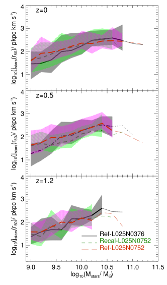
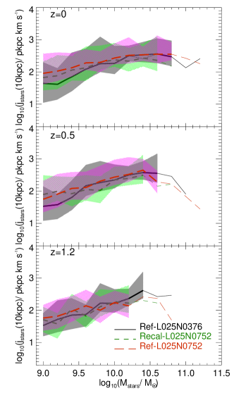
Figure 16: The $j_{\rm stars}$-stellar mass relation at three redshifts, $z=0,\,0.5\,1.2$, for the Ref-L025N0376, Ref-L025N0752 and Recal-L025N0752 simulations, as labelled. We show the relation with $j_{\rm stars}$ measured within the half mass radius of the stellar component (left panels) and within a fixed aperture of $10$ pkpc. Lines show the median relations, while the shaded regions show the $16^{\rm th}-84^{\rm th}$ percentile ranges. The latter are presented only for bins with $\geq 10$ galaxies. Bins with fewer objects are shown as thin lines.

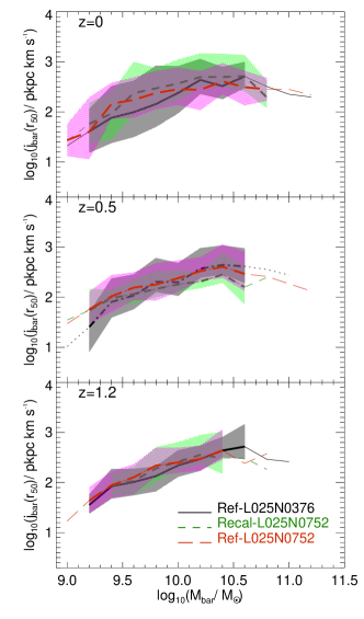
Figure 17: As in the left panels of Fig. 16 but here we show the $j_{\rm bar}$-baryon mass relation.

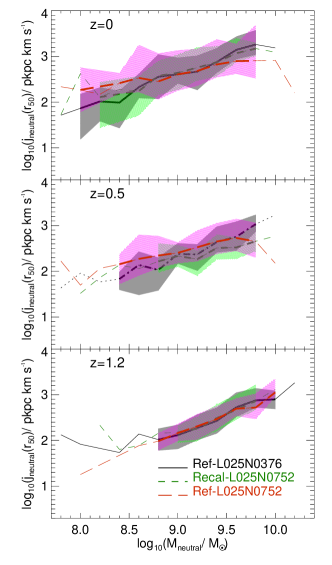
Figure 18: As in the left panels of Fig. 16 but here we show the $j_{\rm neutral}$-neutral gas mass relation.

S15 introduced the concept of ‘strong’ and ‘weak’ convergence tests. Strong convergence refers to the case where a simulation is re-run with higher resolution (i.e. better mass and spatial resolution) adopting exactly the same subgrid physics and parameters. Weak convergence refers to the case when a simulation is re-run with higher resolution but the subgrid parameters are recalibrated to recover, as far as possible, similar agreement with the adopted calibration diagnostic (in the case of eagle, the $z=0.1$ galaxy stellar mass function and disk sizes of galaxies).

S15 introduced two higher-resolution versions of eagle, both in a box of ($25$ cMpc)³ and with $2\times 752^{3}$ particles, Ref-L025N0752 and Recal-L025N0752 (Table 3 shows some details of these simulations). These simulations have better mass and spatial resolution than the intermediate-resolution simulations by factors of $8$ and $2$, respectively. In the case of Ref-L025N0752, the parameters of the sub-grid physics are kept fixed (and therefore comparing with this simulation is a strong convergence test), while the simulation Recal-L025N0752 has $4$ parameters whose values have been slightly modified with respect to the reference simulation (and therefore comparing with this simulation is a weak convergence test).

Here we compare the relation between $j_{\rm stars}$ and stellar mass at three different redshifts in the simulations Ref-L025N0376, Ref-L025N0752 and Recal-L025N0752. Fig. 16 shows the $j_{\rm stars}-M_{\rm stars}$ relation, with $j_{\rm stars}$ measured in two different ways: (i) with all the star particles within a half-mass radius of the stellar component (this is what we do throughout the paper; left panels), and (ii) with all the star particles at a fixed physical aperture of $10$ pkpc (right panels). For the measurement of $j_{\rm stars}(r_{50})$ we find that the simulations Ref-L025N0376 and Ref-L025N0752 produce a very similar relation in the three redshifts analysed (within $\approx 0.15$ dex), $z=0,\,0.5\,1.2$. On the other hand, the Recal-L025N0752 simulation produces a $j_{\rm stars}(r_{50})-M_{\rm stars}$ relation at $z=0$ in very good agreement, but that systematically deviates with redshift. We find that this is due to the difference in the predicted stellar mass-$r_{50}$ relation between the different simulations. This is clear from the right panels of Fig. 16, where we compare now the $j_{\rm stars}(10\rm\,pkpc)-M_{\rm stars}$ relation. Here we see that the three simulations are generally consistent throughout redshift. One could argue that the intermediate resolution run, Ref-L025N0376, which corresponds to the resolution we use throughout the paper, tends to produce $j_{\rm stars}(10\rm\,pkpc)$ slightly smaller than the higher resolutions runs Ref-L025N0752 and Recal-L025N075 at $M_{\rm stars}\lesssim 10^{9.5}\,\rm M_{\odot}$. However, the effect is not seen at every redshift we analysed, and thus it could be due to statistical variations (note that the offset is much smaller than the actual scatter around the median). In order to be conservative, we show in the figures of this paper the limit of $M_{\rm stars}=10^{9.5}\,\rm M_{\odot}$, above which we do not see any difference that could make us suspect resolution limitations.

In Figs. 17 and 18 we study the convergence of the relation $j_{\rm bar}-M_{\rm bar}$ and $j_{\rm neutral}-M_{\rm neutral}$ and conclude that the former is converged at $M_{\rm bar}\gtrsim 10^{9.5}\,\rm M_{\odot}$, while the latter is converged at $M_{\rm neutral}\gtrsim 10^{8.5}\,\rm M_{\odot}$.

Appendix B Scaling relations between the angular momentum of galaxy components

Here we present additional scaling relation between $j_{\rm neutral}$, $j_{\rm stars}$, stellar mass and other galaxy properties.

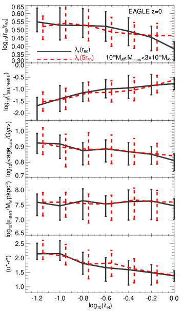
Figure 19: The stellar concentration, $r_{\rm 50}/r_{90}$ (top panel), neutral gas fraction (second panel), stellar age (middle panel), central surface density of stars (fourth panel) and $\rm(u^{*}-r^{*})$ SDSS colour (bottom panel) as a function of $\lambda_{\rm R}$, measured within $r_{50}$ (solid lines) and $5\,r_{50}$ (dashed lines), for galaxies in eagle at $z=0$ with $10^{10}\rm\,M_{\odot}<M_{\rm stars}<3\times 10^{10}\,\rm M_{\odot}$. The lines show the medians with errorbars encompassing the $16^{\rm th}$ to $84^{\rm th}$ percentile ranges.

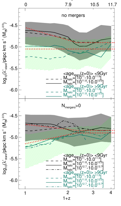
Figure 20: The value of $\lambda^{\prime}_{\rm stars}\equiv j_{\rm stars}(r_{50})/M^{2/3}_{\rm stars}$ as a function of redshift in eagle, for individual central galaxies hosted by halos in the mass ranges labelled in the figure (in units of $\rm M_{\odot}$) at $z=0$, and in two bins of $\langle\rm age_{\rm stars}\rangle$ at $z=0$, $\langle\rm age_{\rm stars}\rangle<9\,\rm Gyr$ (black lines) and $\langle\rm age_{\rm stars}\rangle>9\,\rm Gyr$ (green lines). The top panel shows the subsample of the galaxies above that never suffered a galaxy merger, while in the bottom panel we show those that had a least $1$ merger. The shaded regions show $25^{\rm th}-75^{\rm th}$ percentile ranges, but only for the halo mass range $10^{11.8}\,\rm M_{\odot}\leq M_{\rm halo}\leq 10^{12.3}\,\rm M_{\odot}$. The evolutionary tracks of Fig. 13 are shown as dotted lines.

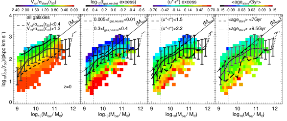
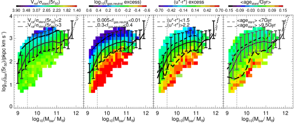
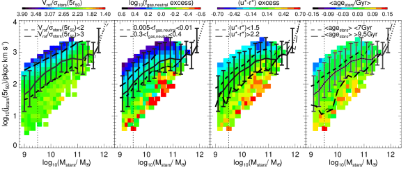
Figure 21: Top panels: As Fig. 1 but for $j_{\rm bar}(r_{\rm 50})$ as a function of the baryon mass (stars plus neutral gas) at $z=0$. Middle panels: As in the top panels but for $j_{\rm bar}(5r_{\rm 50})$. Bottom panels: As Fig. 1 but for $j_{\rm stars}(5r_{\rm 50})$.

In eagle we find that several galaxy properties that trace morphology are related to $\lambda_{\rm R}$, which is used to define slow and fast rotators in the literature (Emsellem et al., 2007). Fig. 19 shows that at a given stellar mass, the neutral gas fraction, the stellar concentration, stellar age, and $\rm(u^{*}-r^{*})$ colour are correlated with $\lambda_{\rm R}$. The latter is directly proportional to $j_{\rm stars}$ and thus it is expected that all these quantities correlate with $j_{\rm stars}$. We do not find a relation between $\mu_{\rm stars}$ and $\lambda_{\rm R}$, and indeed $\mu_{\rm stars}$ is poorly correlated with the positions of galaxies in the $j_{\rm stars}$-stellar mass plane.

We test how much the average evolutionary tracks identified in $\S$ 5.2.1 are mass-independent by replicating the experiment of Fig. 13 but for galaxies in bins of halo mass. In Fig. 20, we show the evolution of $\lambda^{\prime}_{\rm stars}$ for galaxies hosted in halos of different mass ranges $z=0$, separated into galaxies that never suffered a merger (top panel), and that has at least one merger (bottom panel). In each panel we show the subsamples with a mass-weighted stellar age $\rm\langle age_{\rm stars}\rangle\leq 9\,\rm Gyr$ (solid line) and $\rm\langle age_{\rm stars}\rangle>9\,\rm Gyr$ (dashed line). In addition, as dotted lines we show the average evolutionary tracks found in $\S$ 5.2.1. We find that, although some trends can be noisy, these tracks are a reasonable description of the average behaviour observed for the different halo mass bins.

In the top panels of Fig. 21 we study the $j_{\rm bar}-M_{\rm bar}$ relation, and how the scatter correlates with $V_{\rm rot}/\sigma_{\rm stars}$, $f_{\rm gas,neutral}$, $\rm(u^{*}-r^{*})$ and mass-weighted stellar age. We find that there is a positive correlation between $j_{\rm bar}$ and $M_{\rm bar}$ at $10^{9.5}\,\rm M_{\odot}\lesssim M_{\rm bar}\lesssim 10^{10.7}\,\rm M_{\odot}$, with a slope that is close to the theoretical expectations of $j\propto M^{2/3}$ in a CDM universe (see $\S$ 3). However, at higher baryon masses, the relation flattens. The flattening is mainly driven by galaxy merger activity, which is seen from the relation $j_{\rm stars}$ and $j_{\rm bar}$ with stellar mass for galaxies that have undergone different numbers of galaxy mergers (Fig. 2). This will be discussed in detail in an upcoming paper (Lagos et al. in prep.). We find that the scatter in the $j_{\rm bar}$-$M_{\rm bar}$ relation is well correlated with $V_{\rm rot}/\sigma_{\rm stars}$, $f_{\rm gas,neutral}$, $\rm(u^{*}-r^{*})$ and $\rm\langle\rm age_{\rm stars}\rangle$. We did not find any clear correlation between the positions of galaxies in the $j_{\rm bar}-M_{\rm bar}$ plane and the stellar concentration, $r_{90}/r_{50}$, or the central surface density of stars, and thus we do not show them here. The middle panels of Fig. 21 show the $j_{\rm bar}-M_{\rm bar}$ relation with $j_{\rm bar}$ measured within $5\times r_{50}$, for galaxies with $M_{\rm stars}>10^{9}\,\rm M_{\odot}$ at $z=0$ in eagle. We again find here that the trends seen in Fig. 21 are preserved even if we measure $j$ out to large radii.

The bottom panels of Fig. 21 show the $j_{\rm stars}-M_{\rm stars}$ relation with $j_{\rm stars}$ measured within $5\times r_{50}$, for galaxies with $M_{\rm stars}>10^{9}\,\rm M_{\odot}$ at $z=0$ in eagle. We colour the plane by the median $\lambda_{\rm R}(5\,r_{50})$ (left panel), $f_{\rm gas,neutral}$ (middle left panel), (u*-r*) colour (middle right panel) and mass-weighted stellar age (right panel). Here we see that the trends analysed in $\S$ 4 are also found when we perform the study out to large radii. The main difference with Fig. 1 is that the trend with $f_{\rm gas,neutral}$ is stronger when we measure $j_{\rm stars}$ within $5\times r_{50}$.

References

- Bacon et al. (2001) Bacon R., Copin Y., Monnet G., Miller B. W., Allington-Smith J. R., Bureau M., Carollo C. M., Davies R. L. et al, 2001, MNRAS, 326, 23
- Baes et al. (2011) Baes M., Verstappen J., De Looze I., Fritz J., Saftly W., Vidal Pérez E., Stalevski M., Valcke S., 2011, ApJS, 196, 22
- Bahé et al. (2016) Bahé Y. M., Crain R. A., Kauffmann G., Bower R. G., Schaye J., Furlong M., Lagos C., Schaller M. et al, 2016, MNRAS, 456, 1115
- Baugh (2006) Baugh C. M., 2006, Reports on Progress in Physics, 69, 3101
- Benson (2010) Benson A. J., 2010, Phys. Rep., 495, 33
- Bernardi et al. (2010) Bernardi M., Shankar F., Hyde J. B., Mei S., Marulli F., Sheth R. K., 2010, MNRAS, 404, 2087
- Bryant et al. (2015) Bryant J. J., Owers M. S., Robotham A. S. G., Croom S. M., Driver S. P., Drinkwater M. J., Lorente N. P. F., Cortese L. et al, 2015, MNRAS, 447, 2857
- Cappellari et al. (2011a) Cappellari M., Emsellem E., Krajnović D., McDermid R. M., Scott N., Verdoes Kleijn G. A., Young L. M., Alatalo K. et al, 2011a, MNRAS, 413, 813
- Cappellari et al. (2011b) Cappellari M., Emsellem E., Krajnović D., McDermid R. M., Serra P., Alatalo K., Blitz L., Bois M. et al, 2011b, MNRAS, 416, 1680
- Cappellari et al. (2013) Cappellari M., McDermid R. M., Alatalo K., Blitz L., Bois M., Bournaud F., Bureau M., Crocker A. F. et al, 2013, MNRAS, 432, 1862
- Catelan & Theuns (1996a) Catelan P., Theuns T., 1996a, MNRAS, 282, 436
- Catelan & Theuns (1996b) —, 1996b, MNRAS, 282, 455
- Cole et al. (2000) Cole S., Lacey C. G., Baugh C. M., Frenk C. S., 2000, MNRAS, 319, 168
- Cortese et al. (2016) Cortese L., Fogarty L. M. R., Bekki K., van de Sande J., Couch W., Catinella B., Colless M., Obreschkow D. et al, 2016, ArXiv:1608.00291
- Crain et al. (2016) Crain R. A., Bahe Y. M., Lagos C. d. P., Rahmati A., Schaye J., McCarthy I. G., Marasco A., Bower R. G. et al, 2016, ArXiv:1604.06803
- Crain et al. (2015) Crain R. A., Schaye J., Bower R. G., Furlong M., Schaller M., Theuns T., Dalla Vecchia C., Frenk C. S. et al, 2015, MNRAS, 450, 1937
- Croom et al. (2012) Croom S. M., Lawrence J. S., Bland-Hawthorn J., Bryant J. J., Fogarty L., Richards S., Goodwin M., Farrell T. et al, 2012, MNRAS, 421, 872
- Danovich et al. (2015) Danovich M., Dekel A., Hahn O., Ceverino D., Primack J., 2015, MNRAS, 449, 2087
- Doi et al. (2010) Doi M., Tanaka M., Fukugita M., Gunn J. E., Yasuda N., Ivezić Ž., Brinkmann J., de Haars E. et al, 2010, AJ, 139, 1628
- Dolag et al. (2009) Dolag K., Borgani S., Murante G., Springel V., 2009, MNRAS, 399, 497
- Doroshkevich (1970) Doroshkevich A. G., 1970, Astrophysics, 6, 320
- Dubois et al. (2014) Dubois Y., Pichon C., Welker C., Le Borgne D., Devriendt J., Laigle C., Codis S., Pogosyan D. et al, 2014, MNRAS, 444, 1453
- Dwek (1998) Dwek E., 1998, ApJ, 501, 643
- Emsellem et al. (2011) Emsellem E., Cappellari M., Krajnović D., Alatalo K., Blitz L., Bois M., Bournaud F., Bureau M. et al, 2011, MNRAS, 414, 888
- Emsellem et al. (2007) Emsellem E., Cappellari M., Krajnović D., van de Ven G., Bacon R., Bureau M., Davies R. L., de Zeeuw P. T. et al, 2007, MNRAS, 379, 401
- Fall (1983) Fall S. M., 1983, in IAU Symposium, Vol. 100, Internal Kinematics and Dynamics of Galaxies, Athanassoula E., ed., pp. 391–398
- Fall & Efstathiou (1980) Fall S. M., Efstathiou G., 1980, MNRAS, 193, 189
- Fall & Romanowsky (2013) Fall S. M., Romanowsky A. J., 2013, ApJ, 769, L26
- Feldmann et al. (2011) Feldmann R., Carollo C. M., Mayer L., 2011, ApJ, 736, 88
- Furlong et al. (2015a) Furlong M., Bower R. G., Crain R. A., Schaye J., Theuns T., Trayford J. W., Qu Y., Schaller M. et al, 2015a, ArXiv:1510.05645
- Furlong et al. (2015b) Furlong M., Bower R. G., Theuns T., Schaye J., Crain R. A., Schaller M., Dalla Vecchia C., Frenk C. S. et al, 2015b, MNRAS, 450, 4486
- Genel et al. (2015) Genel S., Fall S. M., Hernquist L., Vogelsberger M., Snyder G. F., Rodriguez-Gomez V., Sijacki D., Springel V., 2015, ApJ, 804, L40
- Governato et al. (2010) Governato F., Brook C., Mayer L., Brooks A., Rhee G., Wadsley J., Jonsson P., Willman B. et al, 2010, Nature, 463, 203
- Guedes et al. (2011) Guedes J., Callegari S., Madau P., Mayer L., 2011, ApJ, 742, 76
- Jesseit et al. (2009) Jesseit R., Cappellari M., Naab T., Emsellem E., Burkert A., 2009, MNRAS, 397, 1202
- Kauffmann et al. (1993) Kauffmann G., White S. D. M., Guiderdoni B., 1993, MNRAS, 264, 201
- Kaufmann et al. (2007) Kaufmann T., Mayer L., Wadsley J., Stadel J., Moore B., 2007, MNRAS, 375, 53
- Kelvin et al. (2012) Kelvin L. S., Driver S. P., Robotham A. S. G., Hill D. T., Alpaslan M., Baldry I. K., Bamford S. P., Bland-Hawthorn J. et al, 2012, MNRAS, 421, 1007
- Krajnović et al. (2013a) Krajnović D., Alatalo K., Blitz L., Bois M., Bournaud F., Bureau M., Cappellari M., Davies R. L. et al, 2013a, MNRAS, 432, 1768
- Krajnović et al. (2011) Krajnović D., Emsellem E., Cappellari M., Alatalo K., Blitz L., Bois M., Bournaud F., Bureau M. et al, 2011, MNRAS, 414, 2923
- Krajnović et al. (2013b) Krajnović D., Karick A. M., Davies R. L., Naab T., Sarzi M., Emsellem E., Cappellari M., Serra P. et al, 2013b, MNRAS, 433, 2812
- Kravtsov (2013) Kravtsov A. V., 2013, ApJ, 764, L31
- Lagos et al. (2015) Lagos C. d. P., Crain R. A., Schaye J., Furlong M., Frenk C. S., Bower R. G., Schaller M., Theuns T. et al, 2015, MNRAS, 452, 3815
- Lagos et al. (2016) Lagos C. d. P., Theuns T., Schaye J., Furlong M., Bower R. G., Schaller M., Crain R. A., Trayford J. W. et al, 2016, MNRAS, 459, 2632
- Lintott et al. (2008) Lintott C. J., Schawinski K., Slosar A., Land K., Bamford S., Thomas D., Raddick M. J., Nichol R. C. et al, 2008, MNRAS, 389, 1179
- McAlpine et al. (2015) McAlpine S., Helly J. C., Schaller M., Trayford J. W., Qu Y., Furlong M., Bower R. G., Crain R. A. et al, 2015, ArXiv:1510.01320
- Mo et al. (1998) Mo H. J., Mao S., White S. D. M., 1998, MNRAS, 295, 319
- Naab et al. (2014) Naab T., Oser L., Emsellem E., Cappellari M., Krajnović D., McDermid R. M., Alatalo K., Bayet E. et al, 2014, MNRAS, 444, 3357
- Navarro & Steinmetz (2000) Navarro J. F., Steinmetz M., 2000, ApJ, 538, 477