Linking long-term planetary $N$-body simulations with periodic orbits: application to white dwarf pollution

Abstract

Mounting discoveries of debris discs orbiting newly-formed stars and white dwarfs (WDs) showcase the importance of modeling the long-term evolution of small bodies in exosystems. WD debris discs are in particular thought to form from very long-term (0.1-5.0 Gyr) instability between planets and asteroids. However, the time-consuming nature of $N$-body integrators which accurately simulate motion over Gyrs necessitates a judicious choice of initial conditions. The analytical tools known as periodic orbits can circumvent the guesswork. Here, we begin a comprehensive analysis directly linking periodic orbits with $N$-body integration outcomes with an extensive exploration of the planar circular restricted three-body problem (CRTBP) with an outer planet and inner asteroid near or inside of the $2$:$1$ mean motion resonance. We run nearly 1000 focused simulations for the entire age of the Universe (14 Gyr) with initial conditions mapped to the phase space locations surrounding the unstable and stable periodic orbits for that commensurability. In none of our simulations did the planar CRTBP architecture yield a long-timescale ($\gtrsim 0.25$% of the age of the Universe) asteroid-star collision. The pericentre distance of asteroids which survived beyond this timescale ($\approx 35$ Myr) varied by at most about 60%. These results help affirm that collisions occur too quickly to explain WD pollution in the planar CRTBP $2$:$1$ regime, and highlight the need for further periodic orbit studies with the eccentric and inclined TBP architectures and other significant orbital period commensurabilities.

1 Introduction

Unprecedented images of the rings and dust surrounding HL Tau (ALMA Partnership et al., 2015) provide a glimpse into the complexity of planet formation. At the other end of the life cycle of exosystems, the labile remnant planetary discs orbiting white dwarfs (WDs) are strikingly variable in both brightness and morphology (Wilson et al., 2014; Xu & Jura, 2014; Manser et al., 2016; Wilson et al., 2015; Farihi, 2016). Connecting the future development of systems like HL Tau and the past history of WD debris discs represents an important step towards establishing a unified evolution theory.

This evolution is not limited to planets. Both protoplanetary and WD discs contain dust and potentially asteroids or other small bodies. In fact, asteroids represent the favoured progenitors of WD discs for at least three reasons:

• At least one asteroid has now been observed to be disintegrating in real time around WD 1145+017 (Vanderburg et al., 2015; Alonso et al., 2016; Gänsicke et al., 2016; Rappaport et al., 2016; Xu et al., 2016; Zhou et al., 2016)

• Planets collide with WDs too infrequently (Veras et al., 2013b; Mustill et al., 2014; Veras & Gänsicke, 2015; Veras et al., 2016) as do exo-Oort cloud comets (Alcock et al., 1986; Veras et al., 2014c; Stone et al., 2015)

• Measured bulk compositions in WD atmospheres are incompatible with those from Solar system comets (Zuckerman et al., 2007; Klein et al., 2010, 2011; Gänsicke et al., 2012; Jura et al., 2012; Xu et al., 2013, 2014; Wilson et al., 2016)

Therefore, understanding the interaction between planets and asteroids is paramount for WD planet studies. Further, the wide range of WD cooling ages (the time since the star became a WD) at which metal pollution is observed (up to 5 Gyr; see Farihi et al. 2011 and Koester et al. 2011) necessitate understanding the long-term evolution of planets and asteroids. For a recent review summarizing our current knowledge of the long-term behaviour of planetary systems, see (Davies et al., 2014), and for post-main-sequence systems in particular, see (Veras, 2016).

For the more specific case of an asteroid and planet interacting under the guises of the restricted three-body problem (RTBP), a vast body of literature has covered specific examples and techniques. For example, Holman & Murray (1996) and Murray & Holman (1997) analytically and numerically determined the long-timescale stability of asteroids in or near mean motion resonance (MMR) under the guise of the planar elliptic RTBP, and focused on computing Lyapunov times. Other measures of chaos, such as MEGNO (Hinse et al., 2010), have also been applied to the elliptic RTBP.

$N$-body numerical integrations provide a crucial means of determining orbital evolution, but can be computationally demanding. Alternatively, predictive analytic formulations may yield the desired result more quickly, but their correctness is subject to validation from $N$-body integrations. One example is classic Laplace-Lagrange theory (see Chapter 7 of Murray & Dermott, 1999), which can fail to reproduce quantitative behaviour in exosystems when compared to $N$-body integrations, even when the theory is extended to fourth-order in eccentricity (Veras & Armitage, 2007); other types of extensions yield better results (Libert & Sansottera, 2013). Another example is Lidov-Kozai theory, where differences in its quadrupole-order versus octupole-order accuracy are dramatically highlighted through comparison to $N$-body integrations (e.g. Naoz et al., 2013; Naoz, 2016).

Our purpose in this paper is to begin a series of investigations comparing long-term $N$-body integrations to periodic orbits, which are defined in Section 2. Tsiganis et al. (2002) also relate numerical integrations to periodic orbits, but carry out integrations for just 5 Myr and perform a broad sweep of different period commensurabilities, rather than focusing on one, as we do here. Periodic orbits can be treated as analytical tools which can gather information regarding a system’s dynamics, such as in TBPs. We herein implement the high predictive power of periodic orbits to explore the phase space of a system consisting of a WD, planet and massless asteroid where the planet and asteroid are evolving in or near a particular MMR. Using periodic orbits to remove the guesswork involved in choosing initial conditions can reduce the phase space which needs to be explored and increase the relevance of the simulation suites that are run. We provide definitions and context in Section 2, the results of our numerical simulations in Section 3, a discussion in Section 4 and our conclusion in Section 5.

2 Definitions and context

Now we define a periodic orbit in the planar TBP along with other related, relevant terms. Throughout this work, we will consider only coplanar systems; lifting off this restriction would be a catalyst for future studies. In our TBP, the WD, planet and asteroid have masses of $m_{\rm WD}$, $m_{\rm P}$ and $m_{\rm A}$, and the asteroid is initially closer to the WD than the planet. In Section 2.1, we define periodic orbits. Then we define the closely-related concept of MMR before linking the two in Section 2.2 and finally focusing on the circular RTBP (CRTBP) with a $2$:$1$ internal MMR in Section 2.3.

2.1 Periodic orbits

Consider a suitable frame of reference that is centred on the centre of mass of the WD and the planet and rotated, in order for the periodic orbits to be defined and the degrees of freedom to be subsequently reduced through the angular momentum integral (see e.g. Hadjidemetriou, 1975). Degrees of freedom are defined here as the set $\textbf{Q}(t)$ of positions and velocities of both the planet and asteroid. A periodic orbit is a map $\textbf{Q}(0)=\textbf{Q}(T)$, where the orbit’s period $T$ satisfies $t=kT$, and $k\geq 1$ is an integer. Note that $T$ does not necessarily represent the orbital period of the planet nor the asteroid.

Given the resulting equations of motion, the system can remain invariant under certain transformations. As additional restrictions on this system are imposed, the number of degrees of freedom decreases. For example, the periodicity conditions will determine if the periodic orbit is classified as symmetric or asymmetric. In the planar CRTBP – where the asteroid is considered massless and the planet and WD are on circular orbits – the number of degrees of freedom for symmetric and asymmetric periodic orbits is only 2 and 3, respectively (see Antoniadou et al., 2011).

A periodic orbit coincides with a fixed or periodic point on a Poincaré surface of section. This fixed point can be represented by a given set $\textbf{Q}(0)$. This representation is the crucial link to initial conditions that supply periodic orbits with predictive power. Then, through a process known as monoparametric continuation (see e.g. Hénon, 1997; Hadjidemetriou, 1975), these fixed points can be linked together. The result are smooth curves known as characteristic curves, or families, of periodic orbits. In physical coordinate or orbital element phase space plots, these smooth curves act as the visual manifestation of periodic orbits and provide deep insight into the TBP, illustrating where a three-body system may be stable, or not, over long timescales. In fact, periodic orbits can be classified as “stable” or “unstable” based on a linear stability analysis (Marchal, 1990). An important property of stable symmetric periodic orbits is that the apsidal angle difference precesses about either $0^{\circ}$ (alignment) or $180^{\circ}$ (anti-alignment). It still precesses for asymmetric periodic orbits, but about other angles. The resonant angles librate in a similar manner (for details, see e.g. Antoniadou, 2016). These angles rotate if the periodic orbits are unstable. The key goal of this work is to explore how this classification corresponds to the long-term stability of planet-asteroid systems.

In Hamiltonian systems, stable periodic orbits are surrounded by invariant tori in their neighbourhood in phase space, where the motion is regular and quasi-periodic. On the other hand, homoclinic webs are formed in the vicinity of the unstable periodic orbits, which trigger chaotic motion. In the case of weak chaos, the orbits evolve with some irregularity in the oscillations of orbital elements and a significant change in the configuration of the system is not apparent. If a system is located in strongly chaotic regions, it will eventually destabilize, exhibiting collisions or escape. Thus, the long-term stability of a system can be guaranteed if it resides in a stability domain in phase space buttressed by families of stable periodic orbits.

Here, we consider these periodic orbits in the context of long-term $N$-body simulations.

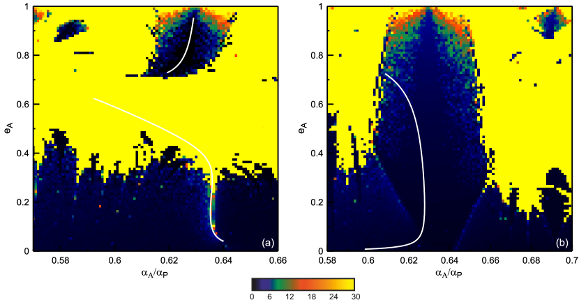
Figure 1: Families of periodic orbits (white curves) for the $2$:$1$ planar CRTBP where in panel (a) $\omega_{\rm A}=M_{\rm A}=180^{\circ}$ and in panel (b) $\omega_{\rm A}=M_{\rm A}=0^{\circ}$. The background colours refer to the level of order in the phase space of the system by illustrating the logarithmic value of the Detrended Fast Lyapunov Indicator (DFLI). The families of stable periodic orbits in both panels reside in the dark regions, and the family of the unstable ones resides in the light region in panel (a).

2.2 Link between periodic orbits and resonances (MMRs)

Because periodic orbits rely on repeating configurations, these orbits are intrinsically linked to MMRs.

An MMR is a class of dynamical states. MMRs have been extensively invoked and studied (see e.g. Varadi, 1999; Laughlin et al., 2011; Haghighipour et al., 2003; Voyatzis & Hadjidemetriou, 2005; Michtchenko et al., 2006; Antoniadou et al., 2011; Antoniadou & Voyatzis, 2013, 2014; Antoniadou et al., 2014). The word commensurability is often used in a similar context with a similar definition, although the difference between a simple period ratio and the exact definition of resonance can have significant implications for the discovery and characterization of exoplanets (Agol et al., 2005; Veras et al., 2011b; Veras & Ford, 2012; Nesvorný et al., 2013; Armstrong et al., 2015).

Direct mathematical definitions of MMRs sometimes start with the time derivative of an angle that appears in a gravitational disturbing function (e.g. pg. 331 of Murray & Dermott, 1999) or a Hamiltonian normal form expanded out to a finite perturbation order (e.g. pg. 57 of Morbidelli, 2002a). The ability of a critical (or resonant) angle to librate (or, oscillate) rather than circulate is a hallmark of many definitions of resonance (see e.g. Beaugé et al., 2003; Michtchenko et al., 2008). Other definitions incorporate the trajectories in phase space between separatricies of a given integrable model. One fundamental problem with definitions that rely on the expansions (of e.g. potentials in Lagrange’s Planetary Equations) about particular values of orbital elements is that the order of the expansion represents a poor metric for accuracy and possibly convergence (Veras, 2007). One limitation of using librations in definitions of resonance is that a libration angle, centre, amplitude and timescale must all be defined (Veras & Ford, 2010). Alternatively, a Hamiltonian form defined by just a few small perturbation terms might necessitate constraining the ranges of orbital elements.

Periodic orbits and MMRs are linked through $T$. The condition for a periodic orbit of period T to exist, $\textbf{Q}(0)=\textbf{Q}(T)$, requires that an admissible value of $T$ is used. Often, these values are associated to multiples of the orbital periods of the planet and asteroid such that the ratio of those multiples corresponds to an orbital period commensurability $\frac{T_{\rm planet}}{T_{\rm asteroid}}=\frac{p+q}{p}=$ rational, $q$ being the order of the MMR (e.g. $2$:$1$, $3$:$1$).

Generally families of periodic orbits are generated by bifurcation points. However, there exist isolated families that do not bifurcate from periodic orbits of other families. Additionally, some MMRs do not admit particular symmetries of periodic orbits. For example, Beaugé (1994) and Voyatzis et al. (2005) indicated that asymmetric periodic orbits do not exist in the CRTBP in internal resonances (where the asteroid is the inner body), but rather only in external resonances (where the asteroid is the outer body). Also, in the spatial TBP, spatial periodic orbits of a given MMR may correspond to inclination-type resonances (Thommes & Lissauer, 2003; Lee & Thommes, 2009; Voyatzis et al., 2014; Namouni & Morais, 2015) as well as the more widely-studied eccentricity-type resonances.

2.3 $2$:$1$ circular restricted three-body problem (CRTBP)

In this paper, we focus on the families of periodic orbits given by the internal $2$:$1$ resonance in the planar CRTBP. For this commensurability and setup, one can find two symmetric periodic orbits through which monoparametric continuation will yield two different branches of families: one stable branch, and one unstable branch. The unstable branch contains two families (see description below), and the stable branch contains one family, making a total of three families.

The two branches correspond to different orbital architectures, i.e. when the asteroid is at pericentre ($\omega_{\rm A}=0^{\circ}$) or apocentre ($\omega_{\rm A}=180^{\circ}$). In both cases, $M_{\rm A}=\omega_{\rm A}$. The variables $M_{\rm A}$ and $\omega_{\rm A}$ are the asteroid’s initial mean anomaly and argument of pericentre. Examples of generation, survival (see Poincaré-Birkhoff theorem) and continuation of families of periodic orbits from the unperturbed ($m_{P}=0$) to the perturbed ($m_{P}>0$) restricted case can be found in Bozis & Hadjidemetriou (1976), Hadjidemetriou (1984) and Hadjidemetriou (1993).

We can visualize these families with projections on the $(a_{\rm A}/a_{\rm P},e_{\rm A})$ plane, where $a_{\rm A}$ and $e_{\rm A}$ refer to the initial semimajor axis and eccentricity of the asteroid, and $a_{\rm P}$ is the initial semimajor axis of the planet.

Figure 1 illustrates these projections when $\omega_{\rm A}=M_{\rm A}=180^{\circ}$ (left panel) and $\omega_{A}=M_{\rm A}=0^{\circ}$ (right panel) with white curves. In Fig. 1a the branch corresponding to the initial location of the asteroid at apocentre is depicted. This branch is divided, via a region of close encounters between the planet and the asteroid, into two families (separate white curves), which consist of unstable symmetric periodic orbits (lower curve) and stable symmetric periodic orbits (upper curve). The curve in Fig. 1b is the branch of family of stable symmetric periodic orbits corresponding to the initial location of the asteroid at pericentre.

None of these curves can be fit with simple empirical formulae, and their seemingly-arbitrary nature hint at the complexity of the planar $2$:$1$ CRTBP. For example, the curves never reach $e_{\rm A}=0$; a gap is formed during continuation from the unperturbed to perturbed case, because of the order of the resonance. For additional details, please see e.g., Voyatzis & Hadjidemetriou (2005), Hadjidemetriou (2006) and Voyatzis et al. (2009).

2.3.1 Detrended Fast Lyapunov Indicator (DFLI)

Plotted in the colourful background behind the lines are contours which indicate the Lyapunov time, a measure of chaos in the system. Specifically, the colour of each point of the plane indicates the logarithmic values of the Detrended Fast Lyapunov Indicator (DFLI) (FLI divided by t) (Froeschlé et al., 1997; Voyatzis, 2008) defined as

$$DFLI(t)=\frac{1}{t}max\left\{\left|\xi_{1}(t)\right|,\left|\xi_{2}(t)\right|\right\},$$

where $\xi_{i}$ are the deviation vectors of the orbit (initially orthogonal) computed after numerical integration of the variational equations of the system for $t_{\rm max}=2.5\times 10^{5}$ years for each initial condition. These contours are not the result of full $N$-body integrations, but rather provide a quick and efficient representation of the phase space. For regular orbits this indicator tends to a constant value, whereas for irregular orbits the indicator increases exponentially over time taking very large values (see Fig. 2 for a demonstration). On the DFLI maps in Fig. 1 and thereafter, dark-coloured regions indicate regular orbits, whereas regions of pale colour represent the the ones where chaotic nature is detected. The integration of the systems was terminated when the index exceeded the value $10^{30}$ and the orbit was accordingly classified (see also the coloured bar in Fig. 1).

DFLI maps are not direct substitutes for $N$-body numerical integrations, and in particular long-term $N$-body numerical integrations. Like periodic orbits, DFLI maps represent tools that can help motivate the initial conditions for $N$-body simulations.

The correspondence between the DFLI maps and periodic orbits themselves in both panels of Fig. 1 is robust. Phase space is built around the periodic orbits given their linear stability. The families of stable periodic orbits are located entirely within dark-coloured regions and constitute the backbone of stability domains, and the families of unstable periodic orbits are located entirely within pale-coloured regions (see also Antoniadou & Voyatzis, 2016).

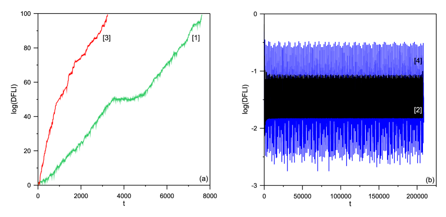
Figure 2: Evolution of the Detrended Fast Lyapunov Indicator (DFLI) for four particular systems: [1] green line, panel a: centred on an unstable periodic orbit from Fig. 1a corresponding to ($a_{\rm A}/a_{\rm P}=0.62498102$, $e_{A}=0.4563692$, and $\omega_{\rm A}=M_{\rm A}=180^{\circ}$), [2] black line, panel b: centred on a stable periodic orbit from Fig. 1a corresponding to ($a_{\rm A}/a_{\rm P}=0.62499828$, $e_{A}=0.7874083$, and $\omega_{\rm A}=M_{\rm A}=180^{\circ}$), [3] red line, panel a: in the vicinity of an unstable periodic orbit, corresponding to ($a_{\rm A}/a_{\rm P}=0.625200$, $e_{A}=0.629990$, and $\omega_{\rm A}=M_{\rm A}=180^{\circ}$), [4] blue line, panel b: in the vicinity of a stable periodic orbit, corresponding to ($a_{\rm A}/a_{\rm P}=0.625200$, $e_{A}=0.873470$, and $\omega_{\rm A}=M_{\rm A}=0^{\circ}$). The DFLI suggests that the first and third systems are irregular or chaotic, and that the second and fourth are regular, or stable.

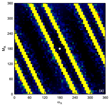
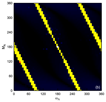
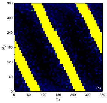
Figure 3: DFLI maps on plane $(\omega_{\rm A},M_{\rm A})$ for (panel a, with $a_{\rm A}/a_{\rm P}=0.627517$ and $e_{\rm A}=0.864125$): a system which intersects with a stable periodic orbit at $\omega_{\rm A}=M_{\rm A}=180^{\circ}$, (panel b, with $a_{\rm A}/a_{\rm P}=0.634690$ and $e_{\rm A}=0.358225$): a system which intersects with an unstable periodic orbit at $\omega_{\rm A}=M_{\rm A}=180^{\circ}$, and (panel c, with $a_{\rm A}/a_{\rm P}=0.620572$ and $e_{\rm A}=0.600409$): a system which intersects with a stable periodic orbit at $\omega_{\rm A}=M_{\rm A}=0^{\circ}$. The periodic orbits are depicted by white circles. These plots reveal how regions of chaotic evolution can be tightly constrained in narrow strips in phase space.

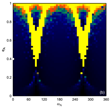
Figure 4: DFLI maps on plane $(\omega_{\rm A},e_{\rm A})$ for (panel a, with $a_{\rm A}/a_{\rm P}=0.625603$ and $M_{\rm A}=180^{\circ}$): a system which intersects with an unstable periodic orbit at $e_{\rm A}=0.456369$, $\omega_{\rm A}=180^{\circ}$, and (panel b, with $a_{\rm A}/a_{\rm P}=0.626144$ and $M_{\rm A}=0^{\circ}$): a system which intersects with a stable periodic orbit at $e_{\rm A}=0.399388$, $\omega_{\rm A}=0^{\circ}$. The periodic orbits are depicted by white circles. These plots reveal the oscillatory shapes of the strips in this phase space in which chaotic motion was detected.

2.3.2 Unraveling phase space

In order to decipher phase space we additionally construct maps on different planes.

In Fig. 3, we keep fixed ($a_{\rm A}/a_{\rm P},e_{\rm A}$), which are provided in the caption, and vary $M_{\rm A}$ and $\omega_{\rm A}$. In panel a, we keep fixed the values of a stable periodic orbit of the stable family of Fig. 1a and as a result, the regular regions are built around the $(\omega_{\rm A},M_{\rm A})=(180^{\circ},180^{\circ})$ and its equivalent configurations. But, one can see in Fig. 1b that this point falls also within the regular region of the stable family of that configuration, i.e. when $(\omega_{\rm A},M_{\rm A})=(0^{\circ},0^{\circ})$. Hence, in Fig. 3a we can also observe the regular regions shaped around the latter configuration and its equivalent ones. In Fig. 3b, we have chosen an unstable periodic orbit of the unstable family of Fig. 1a which as above falls also within the region of stability in Fig. 1b. Hence, we can observe both the very thin (keep in mind that the eccentricity value is low) region of irregular orbits existing in the configuration $(\omega_{\rm A},M_{\rm A})=(180^{\circ},180^{\circ})$ and the regions of regular motion for the configuration $(\omega_{\rm A},M_{\rm A})=(0^{\circ},0^{\circ})$. Again, the repetitive strips of each behaviour are due to the MMR. In Fig. 3c, we have chosen an unstable periodic orbit of the family in Fig. 1a for a greater value of the eccentricity. Thus, in comparison with Fig. 3b the regions where irregular motion was detected are larger.

In Fig. 4 we keep fixed ($a_{\rm A}/a_{\rm P},M_{\rm A}$) and vary $e_{\rm A}$ and $\omega_{\rm A}$ for an unstable (panel a) and stable (panel b) periodic orbit, whose orbital elements are provided in the caption. It is a straightforward observation that both of the structures of regular and irregular orbits seen in Fig. 1 for the two different configurations, i.e. when $(\omega_{\rm A},M_{\rm A})=(180^{\circ},180^{\circ})$ and $(\omega_{\rm A},M_{\rm A})=(0^{\circ},0^{\circ})$ are apparent and being repeated for their equivalent configurations given the $M_{\rm A}$ here, as well. The fixed semimajor axes are almost the same for both panels, whereas the eccentricity in panel a is higher. Thus, we can observe how the regions where irregular evolution was detected via the DFLI are altered.

3 N-body integration setup

Part of the challenge of relating $N$-body simulations to periodic orbits is that the former does not map bijectively to the latter. $N$-body simulations require more input parameters than degrees of freedom in periodic orbits. Also, the development of periodic orbits has historically relied on normalized coordinates, such that, for example, the Gravitational constant and total system mass are both set to unity.

3.1 Scaling factors

The families of periodic orbits have been computed under the assumption that the total mass of the system equals unity, $m_{\rm Star}+m_{\rm P}=1$, where $m_{\rm P}=10^{-3}$. We have to transform this scaling into real units. The invariance of the equations of motion for periodic orbits for different scalings is described in Section 3.2.1.1 of Antoniadou (2014). This analysis reveals that the appropriate scaling factor $\zeta$ is

$$\zeta\equiv\frac{m_{\rm WD}+m_{\rm P}}{1m_{\odot}}.$$ (1)

Now denote orbital elements in $N$-body simulation coordinates with the superscript “N”. Then

$$a_{\rm P}^{\rm(N)} = a_{\rm P}\zeta^{1/3},$$ (2)

$$a_{\rm A}^{\rm(N)} = a_{\rm A}\zeta^{1/3}.$$ (3)

Other orbital elements such as eccentricity, argument of pericentre and mean anomaly remain the same in both coordinate systems. Also, importantly, time is equivalent in both systems. Consequently, the only transformation which needs to take place is with the semimajor axes of both the planet and asteroid.

3.2 Parameter choices

The initial conditions for a $N$-body integrator require a mass, three positions and three velocities to be inserted for each object. In order to detect collisions with the star, the radius of the star must also be specified.

We model evolution during the WD phase only, and hence adopt a fiducial WD mass of $m_{\rm WD}=0.6m_{\odot}$. In order to compare and provide a check on the results from Debes et al. (2012) and Frewen & Hansen (2014) (see Section 5.2), we give our planet a mass that is approximately equal to Jupiter, such that $m_{\rm P}=10^{-3}m_{\odot}$. Consequently, our scaling factor is $\zeta=0.601$. Regarding the radius of the star, we instead wish to use the Roche (or disruption) radius of the star – within which an asteroid would be tidally disrupted. The WD’s Roche radius is dependent on the properties of the asteroid that is being disrupted (see Section 2 of Veras et al. 2014b). Because we do not make assumptions about the internal properties of the asteroids, we simply adopt a fictitious WD radius of $10^{6}$ km $\approx 1.4378R_{\odot}\approx 0.006684$ au. This value conforms well to a conservatively large estimate of the WD’s Roche radius. Any asteroids which enter this radius are flagged as having collided with the WD. With regards to the planet’s radius we used a radius which corresponds to a mass of 0.001 $m_{\odot}$ and a density of 1 $g/cm^{3}$ (so $R_{\rm P}=78,000$ km or 1.09 $R_{\rm Jupiter}$).

Now consider the orbital elements of the planet and asteroid. In the planar TBP, the inclinations and longitudes of ascending nodes of the planet and asteroid can be and are set to zero without loss of generality. In the RTBP, because the asteroid is massless, astrocentric coordinates are equivalent to Jacobi coordinates; the latter was used for periodic orbits. In the CRTBP, because the planet is on a fixed circular orbit, $e_{\rm P}=0$ and the choice of $\omega_{\rm P}$ is irrelevant; we fix it at zero for all simulations. The adopted value of $M_{\rm P}$ determines the planet’s location along its circular orbit. We set $M_{\rm P}=0^{\circ}$ initially in all simulations in order to maintain the same reference geometry.

In all cases we adopt $a_{\rm P}=10$ au, or $a_{\rm P}^{\rm(N)}=8.439009789$ au. The value of $a_{\rm P}$ is realistic because a relatively circular planet at a few to 5 au (like Jupiter) on the main sequence will typically extend its orbit by a factor of 2-3 while maintaining its eccentricity (Veras et al., 2011a) during the GB phases of a Solar-like or slightly more massive star (Duncan & Lissauer, 1998; Schröder & Connon Smith, 2008; Veras & Wyatt, 2012). During the GB phases, a planet out that far is unlikely to be engulfed due to star-planet tides (Kunitomo et al., 2011; Mustill & Villaver, 2012; Adams & Bloch, 2013; Nordhaus & Spiegel, 2013; Villaver et al., 2014; Staff et al., 2016).

The four remaining parameters are then the ones we vary within our suite of numerical simulations: $(a_{\rm A}^{\rm(N)},e_{\rm A},\omega_{\rm A},M_{\rm A})$. We describe and exhibit these choices in Section 4, along with the results.

3.3 Numerical integrator

We perform our numerical simulations with the conservative Bulirsch-Stoer integrator from the modified version of the mercury (Chambers, 1999) integration suite that was used in (Veras & Mustill, 2013). We set the ejection radius at $3\times 10^{5}$ au, which exceeds the Hill ellipsoid for a star in the solar neighbourhood (Veras & Evans, 2013). We adopt a highly accurate tolerance parameter of $10^{-13}$, which allows us to achieve conservation of energy and angular momentum to one part in $10^{-8}-10^{-12}$. The Jacobi constant has typical variations of $10^{-4}$ to $10^{-3}$ (occasionally smaller), but no secular drift. Additionally, the computation of the Tisserand parameter (Bonsor & Wyatt, 2012) for the stable cases helps confirm our results.

The extent of our exploration of this region of phase space is limited by computational resources and integration timescales. We evolve every one of our systems for the lifetime of the Universe (approximately 14 Gyr), corresponding to $\sim 1.1\times 10^{9}$ orbits. Our output resolution is 1 Myr.

4 N-body integration results

In order to explore the 4-dimensional ($a_{\rm A},e_{\rm A},\omega_{\rm A},M_{\rm A}$) phase space, we vary selected pairs of variables in the vicinity of the $2$:$1$ periodic orbits of the planar CRTBP. Our primary interest is connecting the properties of $N$-body simulation outcomes with $(a_{\rm A},e_{\rm A})$ portraits such as those in Fig. 1 (subsection 4.3) and $(M_{\rm A},\omega_{\rm A})$ portraits such as those in Fig. 3 (subsection 4.4). First, however, we comment on some global properties of our simulations (subsections 4.1 and 4.2). We finish this section with some specific examples of system orbital evolution (subsection 4.5).

4.1 Instability timescales

The most important result relating to WD systems regards instability timescales. Across all of our 2847 simulations in the planar CRTBP – including 858 simulations with a stable asteroid that were run for the age of the Universe (14 Gyr) – an asteroid collision with the planet or WD never occurred after 36 Myr. Further, a collision occurred after 1 Myr only 17 times. Further still, many of our simulations, as illustrated below, specifically targeted the regions around unstable periodic orbits. The two main consequences of this finding are (1) the planar CRTBP $2$:$1$ architecture cannot produce long-timescale ($\gtrsim 0.3$% of the age of the Universe) collisions, and (2) that this architecture cannot explain observed rates of WD pollution, in line with the findings of Frewen & Hansen (2014). We will discuss these points more in Section 5.

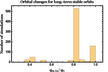
Figure 5: Number of stable systems integrated over 14 Gyr which experience a given maximum change in pericentre distance. Although this distribution is likely reflective of our initial condition choices, the lowest value of about 0.4 is more importantly probably reflective of a global minimum.

4.2 Orbital variations

For studies relevant to WD pollution, a particularly important orbital quantity to measure is how the pericentre distance $q$ changes with time. Let $q_{0}$ represent the initial pericentre distance and $q_{\rm min}$ represent the minimum value of $q$ achieved throughout the simulation. We plot $q_{\rm min}/q_{0}$ in Fig. 5 for all simulations which remained stable and ran for the age of the Universe.

This distribution is naturally highly-dependent on the initial conditions we chose for our simulations. The peak around $q_{\rm min}/q_{0}\approx 0.8$ might simply reflect this dependency. However, because we deliberately attempted to sample key unstable regions of phase space, the minimum ratio attained of $q_{\rm min}/q_{0}\approx 0.4$ is likely to be representative of a global minimum. At least, achieving a value less than about 0.4 is highly unlikely (at the $0.1$% level). A value of 0.4 does not allow the asteroid to get remotely close to the Roche radius of the WD unless the initial pericentre is set to within about $0.02$ au, which is only possible due to a scattering event after the parent star has become a WD.

4.3 Varying pairs of $a_{\rm A}$ and $e_{\rm A}$

Now we directly compare Fig. 1 with similarly-scaled figures that display the results of our long-term integrations (Fig. 6). The top and bottom panels of Fig. 6 correspond to the $\omega_{\rm A}=M_{\rm A}=180^{\circ}$ and $\omega_{\rm A}=M_{\rm A}=0^{\circ}$ cases respectively, like the left and right panels of Fig. 1. The outcomes of the $N$-body integrations are parametrized with different colours, indicating stability (green), escape (orange), collision with the planet (purple) and collision with the star (black). Hence, stability as defined in the N-body simulations does not reflect the long-term stability in the vicinity of stable periodic orbits where the motion is regular, but solely the absence of ejection, collision with the star, or collision with the planet. As we have already mentioned in Section 2.1, chaotic orbits are detected in the neighbourhood of unstable periodic orbits. In some cases, despite the irregularity in the evolution, the initial orbital elements do not change significantly over time and thus, these orbits can be considered as “stable” (see e.g. the examples in Section 4.5).

Hence, our comparisons are inexact: Fig. 1 displays the periodic orbits as well as the DFLI maps, whereas Fig. 6 strictly illustrates qualitative system outcomes. In this figure we observe

1. Distinct blocks of stable systems. The locations of several of these blocks correspond to both regions which are close to stable periodic orbits and to regions containing DFLI regular orbits. One diagonal strip of stable systems, however, on the upper panel of Fig. 6 with $0.5\leq e_{\rm A}\leq 0.7$, is not a solid block, but instead is punctuated with collisional instability. A solid stable block also encompasses the lower tail ($e_{\rm A}\gtrsim 0.4$) of the unstable periodic orbit family (the gray dots represent densely-packed green dots). In this tail, the DLFI includes a mixture of regular and chaotic orbits and does not tend strongly towards either type.

2. Distinct blocks of unstable systems. These blocks do encompass DFLI chaotic orbit regions. One unstable block surrounds the upper portion ($e_{\rm A}\gtrsim 0.4$) of the unstable periodic orbit family. This block features a mix of all types of instability.

3. An inhomogeneous distribution of incidents of star-asteroid and star-planet collisions throughout the phase space. Escape is the dominant form of instability in these systems, and appear in blocks. For the WD case, all collisions occur on too short of a timescale (under 36 Myr) to explain Gyr pollution timescales, regardless of the collision distribution in phase space.

Overall, the correspondence between periodic orbits, DLFI maps, and long-term $N$-body simulations is robust. The low-eccentricity tail of the family of unstable periodic orbits is the most intriguing discrepancy, at first glance. Poincaré surface of sections have on the one hand, revealed that the chaotic regions are bounded and hence, escape cannot occur. On the other hand, they showed that such regions are sensitive to Jupiter’s eccentricity (see e.g. Michtchenko & Ferraz-Mello, 1995; Nesvorný & Ferraz-Mello, 1997; Hadjidemetriou & Voyatzis, 2000). Furthermore, the results of N-body simulations shown in Fig. 6 and depicting the existence of islands of stability within chaotic regions as $a_{\rm A}$ and $e_{\rm A}$ vary in each configuration (i.e. when $\omega_{\rm A}=0^{\circ}$ or $\omega_{\rm A}=180^{\circ}$) are in good agreement with the results presented with surfaces of section in Morbidelli & Moons (1993).

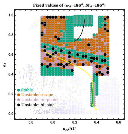
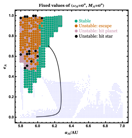
Figure 6: Stability portrait from 14 Gyr $N$-body simulations for fixed $(\omega_{\rm A},M_{\rm A})$. Green spheres indicate stable systems and other dots indicate unstable systems. Orange, purple and black spheres respectively refer to systems where the asteroid escaped, hit the planet, and hit the star. The gray-looking spheres are the result of densely packed green spheres. These plots should be compared with Fig. 1; Families of stable (black) and unstable (yellow) periodic orbits, as well as grid points where $log(DFLI)\leq 1.2$ (pale blue triangular symbols) are overplotted.

4.4 Varying pairs of $M_{\rm A}$ and $\omega_{\rm A}$

Now let us explore this correspondence with the DFLI maps on plane $(M_{\rm A},\omega_{\rm A})$ from Fig. 3. These phase portraits illustrate how stability changes as $M_{\rm A}$ and $\omega_{\rm A}$ are varied, instead of $a_{\rm A}$ and $e_{\rm A}$. These portraits do intersect with both unstable and stable periodic orbits at the points given in that figure caption, but essentially focus on the regions surrounding those orbits. The regions of greatest interest to us are the yellow strips, which are filled with irregular orbits that may become unstable on the timescales we are interested in (Gyr).

We present the results of the $N$-body simulations in Fig. 7. Note that we choose initial conditions for the simulations which roughly correspond to all of the yellow strips in Fig. 3. For each point in each plot in Fig. 7, we ran multiple simulations at different values of $e_{\rm A}$ (provided in the caption). We observe

1. Variations in $e_{\rm A}$ on the order of hundredths often completely changes the outcome of the simulations. In the top plot, at a given point, as $e_{\rm A}$ increases, unstable systems give way to stable systems, because the island of stability is reached (compare Figs. 1a, 3a and 4). These unstable systems predominately feature escape. In the middle plot, at a given point, as $e_{\rm A}$ increases, stable systems give way to unstable systems (which are a mix of escape and collisions), because the chaotic region for the semimajor axis that is fixed begins roughly when $e_{\rm A}>0.4$ (compare Figs. 1a, 3b and 4). In the bottom plot, nearly all the simulations become unstable. However, the character of the instability changes as one varies $e_{\rm A}$. At no point in any of the three plots are all concentric circles the same colour.

2. For a fixed value of $e_{\rm A}$, as one moves along the strips, the outcome of the simulations (stable or unstable) remains largely the same. This trend is apparent in all three plots.

3. Collisions between the asteroid and star are inhomogeneously and infrequently distributed. In no set of concentric circles are more than two coloured black.

4. The two (they are equivalent) exceptions in the bottom plot feature green concentric circles of nearly all stable simulations. They are linked with the outcome that is also seen in the top panel of Fig. 6 for this specific range in the eccentricities and the fixed value of the semimajor axis and justified therein accordingly (compare Figs. 1a, 3c and 4). Also, note how the frequency of green circles decreases as one strays from these equivalent configurations.

Overall, Figs. 3 and 7 demonstrate the importance of the initial orbital angles of the asteroid when determining long-term stability. The role of eccentricity is crucial, and demonstrates predictive power with clear trends.

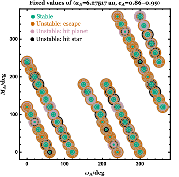
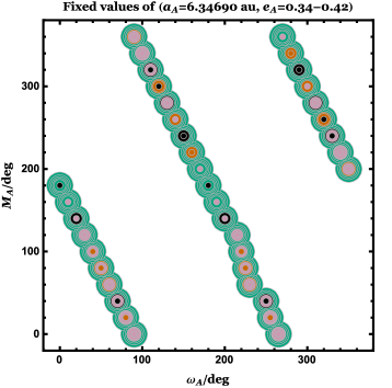
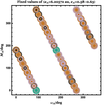
Figure 7: Stability portrait from 14 Gyr $N$-body simulations for fixed $a_{\rm A}$. Dots of different sizes refer to fixed values of $e_{\rm A}$. The largest to smallest dots refer to (top panel) $e_{\rm A}=\left\{0.86,0.88,0.90,0.95,0.97,0.99\right\}$, (middle panel) $e_{\rm A}=\left\{0.34,0.35,0.36,0.38,0.40,0.42\right\}$ and (lower panel) $e_{\rm A}=\left\{0.58,0.59,0.60,0.61,0.62,0.63\right\}$ Colours are as in Fig. 6.

4.5 Specific evolution examples

Even within the confines of the $2$:$1$ planar CRTBP, the asteroid’s osculating orbit may remain nearly static or vary dramatically depending on its initial conditions. Consequently, there is no one representative orbit. Nevertheless, in this subsection we provide a few examples of asteroid evolution in order to at least impart to the reader a flavour of the variety seen across the simulations.

First consider Fig. 8, which exhibits the evolution for three simulations with identical initial orbital parameters (given in the caption) except for $e_{\rm A}$. As $e_{\rm A}$ increases from 0.35 to 0.458 across the three simulations, the qualitative behaviour of the osculating orbit changes in unpredictable ways. The pericentre variation is greatest for the middle panel (from about 1.5 au to 6.0 au). In the top panel, the orbit oscillates back and forth between two different modes of evolution. In the bottom panel, the semimajor axis and pericentre appear to be rigidly bound within differently-sized ranges. When evaluating these plots, please recall that the output resolution for our simulations was 1 Myr.

Figure 9 illustrates a more extreme case, where the asteroid is initially highly eccentric ($e_{\rm A}=0.97$). For this system, we show the evolution of the two $2$:$1$ MMR angles in the right panel (black and blue), along with the evolution of the apsidal angle (red). The black dots clearly librate about $180^{\circ}$ with an amplitude of nearly $50^{\circ}$. The semimajor axis, pericentre and apocentre appear to change little, although the stray purple and green dots below the main stripes indicate brief but potentially dramatic swings from the initial orbit. Inhomogeneities in the stripes themselves (at about 0.4 Gyr and 1.9 Gyr) show up in the right panel as very slow oscillations in the black curves. Alternatively, the dramatically slow circulatory motion indicated by the blue and red curves at about 0.3 Gyr does not appear to manifest itself in the left panel. In order to test if these features are a result of aliasing, we have run 5 additional simulations, each for 7 Gyr. In these simulations, the original output intervals were decreased by factors of 10, 7, 5, 3 and 2. The results demonstrate that the resonance in Fig. 9 appears to be real. In all cases, the angle librates and never deviates from the above-mentioned range.

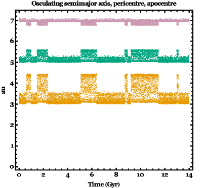
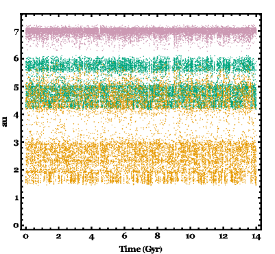
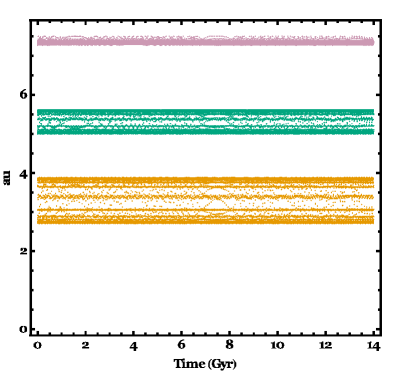
Figure 8: The evolution of the semimajor axis (green), pericentre (orange) and apocentre (purple) of an asteroid in three individual systems. In all three systems, $a_{\rm A}=5.95$ au, $\omega_{\rm A}=0.0^{\circ}$ and $M_{\rm A}=0.0^{\circ}$. In the top, middle and bottom panels, respectively, $e_{\rm A}=\left\{0.35,0.4148,0.458\right\}$. The plots illustrate different qualitative orbital behaviour by changing the eccentricity by about 0.1. Note that the pericentre experiences the greatest variations for the middle eccentricity value.

5 Discussion

In order to place our findings in the proper context, we consider here how they relate to real planetary systems. Partly due to history and to the voluminous and accurate set of available Solar system asteroid data, the vast majority of literature on long-term asteroid evolution is Solar System-specific (e.g. Bottke et al., 2000; Morbidelli, 2002b; O’Brien & Sykes, 2011). Inherent in Solar system studies are assumptions about orbital architectures and radiative physics which do not necessarily apply in extrasolar systems, especially post-main-sequence exosystems.

5.1 Comparison with Solar system studies

The Solar system is different from the planar CRTBP because the former contains more than one planet, and all of the Solar system planets have eccentric orbits which are at least slightly noncoplanar with asteroids and the Sun. Consequently, collisions with the Sun can occur through scattering interactions with multiple planets, leading to a much higher fraction of collisions than in our case (Farinella et al., 1994; Gladman et al., 1997; Minton & Malhotra, 2010). The presence of multiple planets does not, however, preclude the possibility of long-lived (on Gyr timescale) stable “islands" where asteroids can reside in or close to the $2$:$1$ mean motion resonance with Jupiter (Chrenko et al., 2015). Asteroids in such islands may also be shaped by radiation-based perturbations such as the Yarkovsky effect (Brož et al., 2005), which can affect the long-term evolution (Brož & Vokrouhlický, 2008) in ways that are missed in the the planar CRTBP studied herein.

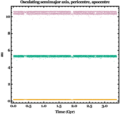
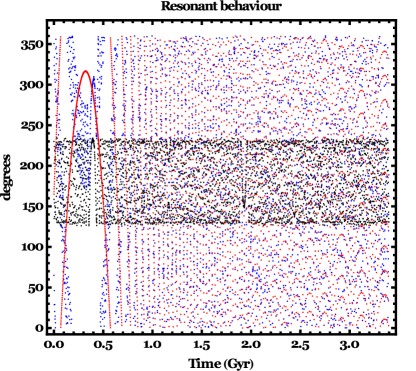
Figure 9: The evolution of an initially and otherwise highly eccentric system ($e_{\rm A}=0.97$) system which exhibits some resonant behaviour. Other initial parameters are $a_{\rm A}=6.2517$ au, $\omega_{\rm A}=195^{\circ}$ and $M_{\rm A}=100^{\circ}$. The left panel illustrates the evolution of the semimajor axis (green), pericentre (orange) and apocentre (purple), and the right panel illustrates the evolution of the two resonant $2$:$1$ angles (black and blue) and the apsidal angle (red). The black points, which correspond to the resonant angle which includes the asteroid’s argument of pericentre, appears to librate about $180^{\circ}$ throughout the 3.5 Gyr of evolution shown, and shows two distinctive features at about 0.4 Gyr and 1.9 Gyr. The circulating apsidal angle is slowest at about 0.3 Gyr.

5.2 Comparison with WD system studies

In contrast, extrasolar systems offer a wide variety of architectures, The majority of all known exosystems contain one exoplanet, leaving open the possibility of the RTBP being widely applicable outside of our Solar system. Individual asteroids are currently undetectable, except in WD systems, where their tidally-shorn innards are observed orbiting WDs or accreting onto them.

Asteroids, comets and planets which orbit stars that leave the main sequence become subject to an assortment of important physical processes whose previous influence was negligible:

1. Stellar mass loss, which causes an outward expansion and possible stretching and breaking of a bound osculating orbit (Omarov, 1962; Hadjidemetriou, 1963; Veras et al., 2011a; Adams et al., 2013; Veras et al., 2013a; Voyatzis et al., 2013)

2. Stellar radius enlargement, leading to engulfment or tidal disruption (Villaver & Livio, 2009; Kunitomo et al., 2011; Mustill & Villaver, 2012; Adams & Bloch, 2013; Nordhaus & Spiegel, 2013; Villaver et al., 2014; Staff et al., 2016),

3. Stellar wind drag, which usually acts in opposition to mass loss (Bonsor & Wyatt, 2010; Dong et al., 2010; Veras et al., 2015a)

4. Variations in stellar luminosity, which lead to YORP-induced fission (Veras et al., 2014a), Yarkovsky-induced dispersion (Veras et al., 2015a), inward drag from radiation pressure and Poynting-Robertson effects (Bonsor & Wyatt, 2010; Dong et al., 2010; Veras et al., 2015b) and sublimation (Veras et al., 2015c)

These effects redistribute surviving bodies and debris in complex and still poorly-understood ways. Regardless, observations reveal that this material somehow is frequently and significantly perturbed close to, and ultimately onto, the resulting WD. In fact planetary remnants are directly detected in the atmospheres of between one quarter and one half of all Milky Way WDs (Zuckerman et al., 2003, 2010; Koester et al., 2014). These signatures are referred to as pollution and are thought to arise from accretion from compact discs (Rafikov, 2011a, b; Metzger et al., 2012; Rafikov & Garmilla, 2012; Wyatt et al., 2014) which are readily observed (e.g. Bergfors et al., 2014; Rocchetto et al., 2014; Wilson et al., 2014; Raddi et al., 2015) and are thought to have formed by the tidal disruption of incoming planetary bodies (Graham et al., 1990; Jura, 2003; Debes et al., 2012; Bear & Soker, 2013; Veras et al., 2014b), such as those disintegrating around WD 1145+017 (Vanderburg et al., 2015). WD pollution reveals the chemical composition of the accreeted bodies (Zuckerman et al., 2007; Gänsicke et al., 2012; Farihi et al., 2013; Jura & Young, 2014; Xu et al., 2014) and consequently provides unambiguous bulk density data about exoplanetary interiors.

Asteroids which pollute WDs must be on highly eccentric orbits because in order to avoid engulfment during the giant branch (GB) stages of stellar evolution, the semimajor axis must be at least a few au. In order to be perturbed into highly eccentric orbits, asteroids need instigators. Three investigations (Bonsor et al., 2011; Debes et al., 2012; Frewen & Hansen, 2014) have dynamically modelled the interaction of asteroids with one planet during the GB phases of evolution, as well as up to 1 Gyr during the WD phase. Bonsor & Veras (2015) considered the consequences of a perturbation by a wide orbit stellar companion, and Payne et al. (2016a, b) determined how liberated moons would contribute to the dynamical architecture.

However, none of those studies included simulations which incorporated the Yarkovsky effect nor stellar wind drag (although see Section 5.1 of Frewen & Hansen 2014), which could represent the dominant drivers of asteroid evolution during the GB phase (Veras et al., 2015a). Therefore, how asteroids evolve during GB evolution, supposing they survive rotational spin-up (Veras et al., 2014a), remains an open question, one that we do not address here.

The RTBP is particularly relevant to these three studies. Debes et al. (2012) suggested that within the RTBP the eccentricity of an asteroid which resides near or inside of an MMR with a planet can gradually increase until the asteroid achieves a WD-grazing orbit. They performed simulations with one planet on an eccentric orbit ($e_{\rm P}=0.0488$) and with asteroids that were inclined with respect to the star-planet plane (J. Debes, private communication) in order to demonstrate their theory. Frewen & Hansen (2014) later explicitly explored how the eccentricity of the planet affects collision rates with the WD when the asteroid was confined to within $0.5^{\circ}$ of the WD-planet plane. They found that $e_{\rm P}>0.02$ is a necessary condition to pollute WDs with a sufficiently high amount of material to extrapolate to observations.

Although the numerical simulations of both studies ran for up to only 1 Gyr, our results affirm theirs and stringently rule out dynamical pollution mechanisms with a single planet on a circular orbit at the $2$:$1$ commensurability. The small inclinations adopted by Frewen & Hansen (2014) suggests that the driver for collisions is planetary eccentricity rather than non-coplanarity. Regardless, undertaking a systematic study for each of these orbital parameters – as well as different commensurabilities – is now required in order to pinpoint the most likely physical origin of long-timescale collisions with the WD. Periodic orbits represent an effective tool for this purpose, especially since so many families have already been computed.

6 Conclusion

We have evaluated the predictive power of periodic orbits and their phase space surroundings to determine the long-term (1-14 Gyr) stability of systems containing one star, one planet and one asteroid in the planar CRTBP. We utilized the three families of periodic orbits which are associated with the $2$:$1$ MMR, such that the asteroid is interior to the planet. Our resource-consuming 14 Gyr simulations revealed good agreement between the final dynamical outcome and the structure of phase space about the periodic orbits. Consequently, researchers can use these orbits as broadly reliable guides to choose sets of initial conditions ($a_{\rm A}^{(\rm N)},e_{\rm A},\omega_{\rm A},M_{\rm A}$) for $N$-body simulations to predict whether a given system will remain stable over the age of the Universe.

Of particular interest for Gyr-old WDs which host circumstellar debris discs and atmospheric metal pollution are unstable planetary systems that feature very late collisions between the asteroid and star. Therefore, in this paper we have focused on unstable cases. Despite this emphasis, in none of our simulations did a collision occur after 36 Myr, thereby providing analytical backing to the findings of Frewen & Hansen (2014) that a circular planet fails to pollute WDs with a sufficient number of asteroids at sufficiently late ages.

References

- Adams et al. (2013) Adams, F. C., Anderson, K. R., & Bloch, A. M. 2013, MNRAS, 432, 438
- Adams & Bloch (2013) Adams, F. C., & Bloch, A. M. 2013, ApJL, 777, LL30
- Agol et al. (2005) Agol, E., Steffen, J., Sari, R., & Clarkson, W. 2005, MNRAS, 359, 567
- Alcock et al. (1986) Alcock, C., Fristrom, C. C., & Siegelman, R. 1986, ApJ, 302, 462
- Alonso et al. (2016) Alonso, R., Rappaport, S., Deeg, H. J., & Palle, E. 2016, A&A, 589, L6
- ALMA Partnership et al. (2015) ALMA Partnership, A. et al. 2015, ApJL, 808, L3
- Antoniadou (2014) Antoniadou, K. I., 2014, Dynamics of planetary systems in resonances: From the planar to the spatial case, PhD thesis, Aristotle University of Thessaloniki, GR
- Antoniadou (2016) Antoniadou, K. I., 2016, Eur. Phys. J. Spec. Top., 225, 1001
- Antoniadou et al. (2011) Antoniadou, K. I., Voyatzis, G., & Kotoulas, T. 2011, IJBC, 21, 2211
- Antoniadou & Voyatzis (2013) Antoniadou, K. I., & Voyatzis, G. 2013, CeMDA, 115, 161
- Antoniadou & Voyatzis (2014) Antoniadou, K. I., & Voyatzis, G. 2014, Ap&SS, 349, 657
- Antoniadou & Voyatzis (2016) Antoniadou, K. I., & Voyatzis, G. 2016, MNRAS, 461, 3822
- Antoniadou et al. (2014) Antoniadou, K. I., Voyatzis, G., & Varvoglis, H. 2014, Proceedings of IAUS, 310, 82, doi:10.1017/S1743921314007893
- Armstrong et al. (2015) Armstrong, D. J., Veras, D., Barros, S. C. C., et al. 2015, A&A, 582, A33
- Beaugé (1994) Beaugé, C. 1994, CeMDA, 60, 225
- Beaugé et al. (2003) Beaugé, C., Ferraz-Mello, S., & Michtchenko, T. A. 2003, ApJ, 593, 1124
- Bear & Soker (2013) Bear, E., & Soker, N. 2013, New Astronomy, 19, 56
- Bergfors et al. (2014) Bergfors, C., Farihi, J., Dufour, P., & Rocchetto, M. 2014, MNRAS, 444, 2147
- Bonsor & Wyatt (2010) Bonsor, A., & Wyatt, M. 2010, MNRAS, 409, 1631
- Bonsor & Wyatt (2012) Bonsor, A., & Wyatt, M. 2012, MNRAS, 420, 2990
- Bonsor et al. (2011) Bonsor, A., Mustill, A. J., & Wyatt, M. C. 2011, MNRAS, 414, 930
- Bonsor & Veras (2015) Bonsor, A., & Veras, D. 2015, MNRAS, 454, 53
- Bottke et al. (2000) Bottke, W. F., Jedicke, R., Morbidelli, A., Petit, J.-M., & Gladman, B. 2000, Science, 288, 2190
- Bozis & Hadjidemetriou (1976) Bozis, G., & Hadjidemetriou, J. D. 1976, Celestial Mechanics, 13, 127
- Brož et al. (2005) Brož, M., Vokrouhlický, D., Roig, F., et al. 2005, MNRAS, 359, 1437
- Brož & Vokrouhlický (2008) Brož, M., & Vokrouhlický, D. 2008, MNRAS, 390, 715
- Chambers (1999) Chambers, J. E. 1999, MNRAS, 304, 793
- Chrenko et al. (2015) Chrenko, O., Brož, M., Nesvorný, D., Tsiganis, K., & Skoulidou, D. K. 2015, MNRAS, In Press, arXiv:1505.04329
- Davies et al. (2014) Davies, M. B., Adams, F. C., Armitage, Chambers, J., Ford, E., Morbidelli, A., Raymond, S. N., Veras, D. 2014, Protostars and Planets VI, 787
- Debes et al. (2012) Debes, J. H., Walsh, K. J., & Stark, C. 2012, ApJ, 747, 148
- Dong et al. (2010) Dong, R., Wang, Y., Lin, D. N. C., & Liu, X.-W. 2010, ApJ, 715, 1036
- Duncan & Lissauer (1998) Duncan, M. J., & Lissauer, J. J. 1998, Icarus, 134, 303
- Farihi et al. (2011) Farihi, J., Dufour, P., Napiwotzki, R., & Koester, D. 2011, MNRAS, 413, 2559
- Farihi et al. (2013) Farihi, J., Gänsicke, B. T., & Koester, D. 2013, Science, 342, 218
- Farihi (2016) Farihi, J. 2016, New Astronomy Reviews, 71, 9
- Farinella et al. (1994) Farinella, P., Froeschlé, C., Froeschlé, C., et al. 1994, Nature, 371, 314
- Frewen & Hansen (2014) Frewen, S. F. N., & Hansen, B. M. S. 2014, MNRAS, 439, 2442
- Froeschlé et al. (1997) Froeschlé, C., Lega, E., & Gonczi, R. 1997, CeMDA, 67, 41
- Gänsicke et al. (2012) Gänsicke, B. T., Koester, D., Farihi, J., et al. 2012, MNRAS, 424, 333
- Gänsicke et al. (2016) Gänsicke, B. T., Aungwerojwit, A., Marsh, T. R., et al. 2016, ApJL, 818, L7
- Gladman et al. (1997) Gladman, B. J., Migliorini, F., Morbidelli, A., et al. 1997, Science, 277, 197
- Graham et al. (1990) Graham, J. R., Matthews, K., Neugebauer, G., & Soifer, B. T. 1990, ApJ, 357, 216
- Hadjidemetriou (1963) Hadjidemetriou, J. D. 1963, Icarus, 2, 440
- Hadjidemetriou (1975) Hadjidemetriou, J. D. 1975, Celestial Mechanics, 12, 155
- Hadjidemetriou (1984) Hadjidemetriou, J. D. 1984, Celestial Mechanics, 34, 379
- Hadjidemetriou (1993) Hadjidemetriou, J. D. 1993, CeMDA, 56, 201
- Hadjidemetriou (2006) Hadjidemetriou, J. D. 2006, CeMDA, 95, 225
- Hadjidemetriou & Voyatzis (2000) Hadjidemetriou J., Voyatzis G., 2000, CeMDA, 78, 137
- Haghighipour et al. (2003) Haghighipour, N., Couetdic, J., Varadi, F., & Moore, W. B. 2003, ApJ, 596, 1332
- Hénon (1997) Hénon, M. 1997, Generating Families in the Restricted Three-Body Problem, Springer-Verlag
- Hinse et al. (2010) Hinse, T. C., Christou, A. A., Alvarellos, J. L. A., & Goździewski, K. 2010, MNRAS, 404, 837
- Holman & Murray (1996) Holman, M. J., & Murray, N. W. 1996, AJ, 112, 1278
- Jura (2003) Jura, M. 2003, ApJL, 584, L91
- Jura et al. (2012) Jura, M., Xu, S., Klein, B., Koester, D., & Zuckerman, B. 2012, ApJ, 750, 69
- Jura & Young (2014) Jura, M., & Young, E. D. 2014, Annual Review of Earth and Planetary Sciences, 42, 45
- Klein et al. (2010) Klein, B., Jura, M., Koester, D., Zuckerman, B., & Melis, C. 2010, ApJ, 709, 950
- Klein et al. (2011) Klein, B., Jura, M., Koester, D., & Zuckerman, B. 2011, ApJ, 741, 64
- Laughlin et al. (2011) Laughlin, G., Chambers, J., & Fischer, D. 2011, ApJ, 579, 455
- Koester et al. (2011) Koester, D., Girven, J., Gänsicke, B. T., & Dufour, P. 2011, A&A, 530, AA114
- Koester et al. (2014) Koester, D., Gänsicke, B. T., & Farihi, J. 2014, A&A, 566, AA34
- Kunitomo et al. (2011) Kunitomo, M., Ikoma, M., Sato, B., Katsuta, Y., & Ida, S. 2011, ApJ, 737, 66
- Lee & Thommes (2009) Lee, M. H., & Thommes, E. W. 2009, ApJ, 702, 1662
- Libert & Sansottera (2013) Libert, A.-S., & Sansottera, M. 2013, Celestial Mechanics and Dynamical Astronomy, 117, 149
- Manser et al. (2016) Manser, C.J., et al. 2016, MNRAS, 455, 4467
- Marchal (1990) Marchal, C. 1990, The three-body problem, Elsevier, Amsterdam
- Metzger et al. (2012) Metzger, B. D., Rafikov, R. R., & Bochkarev, K. V. 2012, MNRAS, 423, 505
- Michtchenko et al. (2006) Michtchenko, T. A., Beaugé, C., & Ferraz-Mello, S. 2006, CeMDA, 94, 411
- Michtchenko et al. (2008) Michtchenko, T. A., Beaugé, C., & Ferraz-Mello, S. 2008, MNRAS, 387, 747
- Michtchenko & Ferraz-Mello (1995) Michtchenko T. A., Ferraz-Mello S. 1995, A&A, 303, 945
- Minton & Malhotra (2010) Minton, D. A., & Malhotra, R. 2010, Icarus, 207, 744
- Morbidelli (2002a) Morbidelli, A. 2002a, Modern celestial mechanics : aspects of solar system dynamics, by Alessandro Morbidelli. London: Taylor & Francis, 2002, ISBN 0415279399
- Morbidelli (2002b) Morbidelli, A. 2002b, Annual Review of Earth and Planetary Sciences, 30, 89
- Morbidelli & Moons (1993) Morbidelli, A., & Moons, M. 1993, Icarus, 102, 316
- Murray & Dermott (1999) Murray, C. D., & Dermott, S. F. 1999, Solar system dynamics. Cambridge Univ. Press, Cambridge
- Murray & Holman (1997) Murray, N., & Holman, M. 1997, AJ, 114, 1246
- Mustill & Villaver (2012) Mustill, A. J., & Villaver, E. 2012, ApJ, 761, 121
- Mustill et al. (2014) Mustill, A. J., Veras, D., & Villaver, E. 2014, MNRAS, 437, 1404
- Naoz (2016) Naoz, S. 2016, ARA&A In Press, arXiv:1601.07175
- Nesvorný & Ferraz-Mello (1997) Nesvorný, D. & Ferraz-Mello, S. 1997, A&A, 320, 672
- Nesvorný et al. (2013) Nesvorný, D., Kipping, D., Terrell, D., et al. 2013, ApJ, 777, 3
- Namouni & Morais (2015) Namouni, F., & Morais, M. H. M. 2015, MNRAS, 446, 1998
- Naoz et al. (2013) Naoz, S., Farr, W. M., Lithwick, Y., Rasio, F. A., & Teyssandier, J. 2013, MNRAS, 431, 2155
- Nordhaus & Spiegel (2013) Nordhaus, J., & Spiegel, D. S. 2013, MNRAS, 432, 500
- O’Brien & Sykes (2011) O’Brien, D. P., & Sykes, M. V. 2011, Solar System Reviews, 163, 41
- Omarov (1962) Omarov, T. B. 1962, Izv. Astrofiz. Inst. Acad. Nauk. Kaz. SSR, 14, 66
- Payne et al. (2016a) Payne, M. J., Veras, D., Holman, M. J., Gänsicke, B. T. 2016a, MNRAS, 457, 217
- Payne et al. (2016b) Payne, M. J., Veras, D., Gänsicke, B. T., Holman, M. J. 2016b, Submitted to MNRAS
- Raddi et al. (2015) Raddi, R., Gänsicke, B. T., Koester, D., Farihi J., Hermes J. J., Scaringi S., Breedt E., Girven J., 2015, MNRAS, 450, 2083
- Rafikov (2011a) Rafikov, R. R. 2011a, MNRAS, 416, L55
- Rafikov (2011b) Rafikov, R. R. 2011b, ApJL, 732, LL3
- Rafikov & Garmilla (2012) Rafikov, R. R., & Garmilla, J. A. 2012, ApJ, 760, 123
- Rappaport et al. (2016) Rappaport, S., Gary, B. L., Kaye, T., et al. 2016, MNRAS, 458, 3904
- Rocchetto et al. (2014) Rocchetto, M., Farihi, J., Gaensicke, B. T., & Bergfors, C. 2014, arXiv:1410.6527
- Schröder & Connon Smith (2008) Schröder, K.-P., & Connon Smith, R. 2008, MNRAS, 386, 155
- Staff et al. (2016) Staff, J. E., De Marco, O., Wood, P., Galaviz, P., & Passy, J.-C. 2016, MNRAS, 458, 832
- Stone et al. (2015) Stone, N., Metzger, B. D., & Loeb, A. 2015, MNRAS, 448, 188
- Thommes & Lissauer (2003) Thommes, E. W., & Lissauer, J. J. 2010, ApJ, 597, 566
- Tsiganis et al. (2002) Tsiganis, K., Varvoglis, H., & Hadjidemetriou, J. D. 2002, Icarus, 159, 284
- Vanderburg et al. (2015) Vanderburg, A., Johnson, J. A., Rappaport, S., et al. 2015, Nature, 526, 546
- Varadi (1999) Varadi, F. 1999, AJ, 118, 2526
- Veras (2007) Veras, D. 2007, Celestial Mechanics and Dynamical Astronomy, 99, 197
- Veras & Armitage (2007) Veras, D., & Armitage, P. J. 2007, ApJ, 661, 1311
- Veras & Ford (2010) Veras, D., & Ford, E. B. 2010, ApJ, 715, 803
- Veras et al. (2011a) Veras, D., Wyatt, M. C., Mustill, A. J., Bonsor, A., & Eldridge, J. J. 2011a, MNRAS, 417, 2104
- Veras et al. (2011b) Veras, D., Ford, E. B., & Payne, M. J. 2011b, ApJ, 727, 74
- Veras & Ford (2012) Veras, D., & Ford, E. B. 2012, MNRAS, 420, L23
- Veras & Wyatt (2012) Veras, D., & Wyatt, M. C. 2012, MNRAS, 421, 2969
- Veras et al. (2013a) Veras, D., Hadjidemetriou, J. D., & Tout, C. A. 2013a, MNRAS, 435, 2416
- Veras et al. (2013b) Veras, D., Mustill, A. J., Bonsor, A., & Wyatt, M. C. 2013b, MNRAS, 431, 1686
- Veras & Mustill (2013) Veras, D., & Mustill, A. J. 2013, MNRAS, 434, L11
- Veras & Evans (2013) Veras, D., & Evans, N. W. 2013, MNRAS, 430, 403
- Veras et al. (2014a) Veras, D., Jacobson, S. A., Gänsicke, B. T. 2014a, MNRAS, 445, 2794
- Veras et al. (2014b) Veras, D., Leinhardt, Z. M., Bonsor, A., & Gänsicke, B. T. 2014b, MNRAS, 445, 2244
- Veras et al. (2014c) Veras, D., Shannon, A., Gänsicke, B. T. 2014c, MNRAS, 445, 4175
- Veras et al. (2015a) Veras, D., Eggl, S., & Gänsicke, B. T. 2015a, In Press, arXiv:1505.01851
- Veras et al. (2015b) Veras, D., Leinhardt, Z.M., Eggl, S., & Gänsicke, B. T. 2015b, In Press, MNRAS, arXiv:1505.06204
- Veras et al. (2015c) Veras, D., Eggl, S., & Gänsicke, B. T. 2015c, In Press, MNRAS, arXiv:1506.07174
- Veras & Gänsicke (2015) Veras, D., Gänsicke, B. T. 2015, MNRAS, 447, 1049
- Veras (2016) Veras, D. 2016, Royal Society Open Science, 3, 150571
- Veras et al. (2016) Veras, D., Mustill, A. J., Gänsicke, B. T., et al. 2016, MNRAS, 458, 3942
- Villaver & Livio (2009) Villaver, E., & Livio, M. 2009, ApJL, 705, L81
- Villaver et al. (2014) Villaver, E., Livio, M., Mustill, A. J., & Siess, L. 2014, ApJ, 794, 3
- Voyatzis (2008) Voyatzis, G. 2008, ApJ, 675, 802
- Voyatzis et al. (2014) Voyatzis, G., Antoniadou, K. I., & Tsiganis, K. 2014, CeMDA 119, 221
- Voyatzis & Hadjidemetriou (2005) Voyatzis, G., & Hadjidemetriou, J. D. 2005, CeMDA, 93, 263
- Voyatzis et al. (2013) Voyatzis, G., Hadjidemetriou, J. D., Veras, D., & Varvoglis, H. 2013, MNRAS, 430, 3383
- Voyatzis et al. (2005) Voyatzis, G., Kotoulas, T., & Hadjidemetriou, J. D. 2005, CeMDA, 91, 191
- Voyatzis et al. (2009) Voyatzis, G., Kotoulas, T., & Hadjidemetriou, J. D. 2009, MNRAS, 395, 2147
- Wilson et al. (2014) Wilson, D. J., Gänsicke, B. T., Koester, D., et al. 2014, MNRAS, 445, 1878
- Wilson et al. (2015) Wilson, D. J., Gänsicke, B. T., Koester, D., et al. 2015, MNRAS, 451, 3237
- Wilson et al. (2016) Wilson, D. J., Gänsicke, B. T., Farihi, J., & Koester, D. 2016, MNRAS In Press, arXiv:1604.03104
- Wyatt et al. (2014) Wyatt, M. C., Farihi, J., Pringle, J. E., & Bonsor, A. 2014, MNRAS, 439, 3371
- Xu et al. (2013) Xu, S., Jura, M., Klein, B., Koester, D., & Zuckerman, B. 2013, ApJ, 766, 132
- Xu et al. (2014) Xu, S., Jura, M., Koester, D., Klein, B., & Zuckerman, B. 2014, ApJ, 783, 79
- Xu & Jura (2014) Xu, S., & Jura, M. 2014, ApJL, 792, L39
- Xu et al. (2016) Xu, S., Jura, M., Dufour, P., & Zuckerman, B. 2016, ApJL, 816, L22
- Zhou et al. (2016) Zhou, G., Kedziora-Chudczer, L., Bailey, J., et al. 2016, arXiv:1604.07405
- Zuckerman et al. (2003) Zuckerman, B., Koester, D., Reid, I. N., Hünsch, M. 2003, ApJ, 596, 477
- Zuckerman et al. (2007) Zuckerman, B., Koester, D., Melis, C., Hansen, B. M., & Jura, M. 2007, ApJ, 671, 872
- Zuckerman et al. (2010) Zuckerman, B., Melis, C., Klein, B., Koester, D., & Jura, M. 2010, ApJ, 722, 725