Tractable Bayesian variable selection: beyond normality
Abstract.
Bayesian variable selection often assumes normality, but the effects of model misspecification are not sufficiently understood. There are sound reasons behind this assumption, particularly for large : ease of interpretation, analytical and computational convenience. More flexible frameworks exist, including semi- or non-parametric models, often at the cost of some tractability. We propose a simple extension of the Normal model that allows for skewness and thicker-than-normal tails but preserves tractability. It leads to easy interpretation and a log-concave likelihood that facilitates optimization and integration. We characterize asymptotically parameter estimation and Bayes factor rates, in particular studying the effects of model misspecification. Under suitable conditions misspecified Bayes factors are consistent and induce sparsity at the same asymptotic rates than under the correct model. However, the rates to detect signal are altered by an exponential factor, often resulting in a loss of sensitivity. These deficiencies can be ameliorated by inferring the error distribution from the data, a simple strategy that can improve inference substantially. Our work focuses on the likelihood and can thus be combined with any likelihood penalty or prior, but here we focus on non-local priors to induce extra sparsity and ameliorate finite-sample effects caused by misspecification. Our results highlight the practical importance of focusing on the likelihood rather than solely on the prior, when it comes to Bayesian variable selection. The methodology is available in R package ‘mombf’.
Keywords: Variable selection, two-piece errors, Bayes factors, model misspecification, robust regression.
1. Introduction
The rise of high-dimensional problems has generated a renewed interest in simple models. Beyond the obvious issue that modest sample sizes limit the number of parameters that can be learned accurately, simple models remain a central choice due to their analytical and computational tractability, ease of interpretation, and the fact that they often work well in practice. There is, however, a pressing need to seek extensions which, while retaining the aforementioned advantages, incorporate additional flexibility and can be studied without unrealistically assuming that the posed model is correct. Ideally such extensions should detect when the added flexibility is not needed so that one can fall back onto simpler models. We focus on canonical variable selection in linear regression from a Bayesian standpoint, although some results may also be useful for penalized likelihood methods. Given that the number of models to consider is exponential in the number of variables, it is highly convenient to adopt error models that lead to fast within-model calculations, e.g. closed forms or fast approximations for the integrated likelihood. Our work is based on two-piece distributions, an easily interpretable family that has a long history and which we fully characterize in the linear model case (synthesizing and extending current results) under model misspecification. Our main contributions are showing that two-piece errors (specifically when applied to the Normal and Laplace families) lead to tractable inference, proposing simple computational algorithms, and characterizing variable selection under model misspecification, including when this likelihood is combined with non-local priors (NLPs, Johnson and Rossell (2010)). We show that in the presence of asymmetries or heavy tails the Normal model incurs a significant loss of power, and propose a formal strategy to detect such departures from normality. When these departures are negligible our model collapses onto Normal errors, for which closed-form expressions are often available.
To fix ideas, we consider the linear regression model
| (1) |
where is the observed outcome for individuals, is an matrix with potential predictors, are regression coefficients and are independent and identically distributed (id) errors (see Section 5.2 for a discussion on non-id errors). The goal is to determine the non-zero coefficients in under an arbitrary data-generating distribution for the ’s, building a framework that remains convenient for large . Let for be variable inclusion indicators and the number of active variables. To consider that residuals may be asymmetric and/or have thicker-than-normal tails denotes the presence of asymmetry ( otherwise) and that of thick tails ( for Normal tails). Thus denotes the assumed model. and are the corresponding submatrix of and subvector of , respectively. We denote the row in and by and .
There are a number of proposals to relax the normality assumption. Within the frequentist literature Wang et al. (2007) proposed median regression with LASSO penalties (LASSO-LAD) and Wang and Li (2009) with rank-based SCAD penalties. Arslan (2012) extended LASSO median regression by weighting observations and Fan et al. (2014) considered adaptive LASSO quantile regression. These approaches are formally connected to assuming either Laplace or asymmetric Laplace errors. There are also model-free M-estimation methods, e.g. combining Huber’s loss with an adaptive LASSO penalty Lambert-Lacroix (2011), sparse trimmed-means LASSO Alfons et al. (2013), and non-negative garrote extensions to induce robustness to outliers Gijbels and Vrinssen (2015). Theoretical characterizations also exist, e.g. Mendelson (2014) proved the consistency and asymptotic normality of high-dimensional M-estimators and Loh (2017) extended the results to generalized M-estimators with non-convex loss functions. Within the Bayesian framework, Gottardo and Raftery (2007) and Wang et al. (2016) consider variable selection after transforming and/or , the former allowing for errors and the latter inducing NLPs on via the transformation’s Jacobian. While certainly interesting, the transformed conditional mean is no longer linear in and parameter interpretation and prior elicitation is less straightforward. Our main interest is in linear predictors with simple error distributions. Along these lines, Yu et al. (2013) proposed Gibbs sampling for model choice in Bayesian quantile regression using a latent scale augmentation, and Yan and Kottas (2015) extended Azzalini’s skew Normal to Laplace errors within Bayesian quantile regression, which leads to easily-implementable MCMC, and induced sparsity via LASSO penalties. Related to our work Rubio and Genton (2016) and Rubio and Yu (2017) employ skew-symmetric and two-piece errors in linear regression, respectively, albeit the set of covariates is fixed and they focus on prediction and censored responses. Yet another possible avenue is to pose highly flexible errors, e.g. Chung and Dunson (2009) set a non-parametric model to simultaneously learn the effect of on the mean and on the shape of the residual distribution. Kundu and Dunson (2014) proposed variable selection with non-parametric symmetric residuals, for which notably Chae et al. (2016) proved high-dimensional model selection consistency and concentration rates under model misspecification. Most Bayesian work uses Markov Chain Monte Carlo (MCMC) for parameter estimation and computation of marginal likelihoods and does not collapse onto the Normal model when warranted by the data, hampering its computational scalability as or grow, further the theoretical study is typically M-closed.
In contrast, we show that simpler parametric error models equipped with efficient analytical approximations to the integrated likelihood achieve selection consistency under model misspecification, and embed these models within a framework that when appropriate collapses onto normality. We also show that model misspecification can markedly decrease the sensitivity to detect truly active variables, e.g. under asymmetry or heavy tails. Our results complement the examples in Grünwald and van Ommen (2014), where the presence of inliers favoured the addition of spurious variables (see also Figure 1 in Kundu and Dunson (2014)). We show that asymptotically misspecified Bayes factors to discard spurious models essentially multiply the correct Bayes factor by a constant term, but when detecting true signals this term is exponential in . That is, asymptotically model misspecification has more serious effects on sensitivity than on false positives. For finite , false positives can be an important issue. We use the example in Grünwald and van Ommen (2014) to illustrate how such finite effects can be reduced by penalizing small coefficients via NLPs (Section 6.2).
Before presenting our approach we clarify our main contributions relative to earlier work in two-piece distributions. Rubio and Steel (2014) showed that Jeffreys priors and their associated posteriors for location-scale two-piece models are improper, and that the (improper) independence Jeffreys prior leads to a proper posterior. Rubio and Yu (2017) extended the study to linear regression, again under improper priors. Unfortunately, improper priors cannot be used for Bayesian model selection as they lead to the well-known Jeffreys-Lindley-Bartlett paradox. There is also literature (e.g. Arellano-Valle et al. (2005)) on MLE consistency and asymptotic normality in the case with no covariates. Checks of the large sample theory technical conditions are however hard to come by, which are non-standard due to the non-existence of certain derivatives. Our two-piece likelihood properties, specifically log-concativity and asymptotic analysis under model misspecification are, to our knowledge, new. As well as our results on Bayes factors, indeed the main theme of our paper: model selection. The M-estimation technical machinery for the theorems is also of interest as an avenue for asymptotic analysis of Bayesian model selection under misspecification. Finally optimization and integration algorithms built on interior-point methods are newly developed here to scale with and . A particular case of our framework provides a new approach to Bayesian quantile regression. We also propose a novel strategy to infer the error model from the data.
The manuscript is structured as follows. Section 2 reviews two-piece distributions and establishes the concavity of the log-likelihood in the asymmetric Normal and Laplace cases. Section 3 proposes a prior formulation based on NLPs that enforces sparsity and discards degrees of asymmetry that are irrelevant in practice. Section 4 tackles maximum likelihood and posterior mode estimation, specifically giving asymptotic distributions and optimization algorithms that capitalize on likelihood tractability. Section 5 outlines a framework to select both variables and the residual distribution, proposes fast approximations to the integrated likelihood and characterizes asymptotically the associated Bayes factors. Section 6 shows results on simulated and experimental data, and Section 7 offers concluding remarks. The supplementary material contains all proofs and further results. R code to reproduce our results is also provided as a supplement to this article.
2. Log-likelihood
We recall the definition of a two-piece distribution for model (1) and predictors .
Definition 1.
A random variable following a two-piece distribution with location , scale and asymmetry has density function
| (2) | |||
where is a symmetric unimodal density with mode at and support on , and .
Two-piece distributions induce asymmetry by (continuously) merging two symmetric densities that have the same mode but different scale parameters , on each side of the mode. Some popular parameterizations are the inverse scale factors for Fernández and Steel (1998) or the epsilon-skew parameterization for Mudholkar and Hutson (2000). We adopt the latter as it leads to orthogonality in the expected log-likelihood hessian between and , also it allows easy interpretation as the total variation distance between and its symmetric counterpart is Dette et al. (2016). Further, a classical skewness coefficient proposed by Arnold-Groeneveld defined as for a univariate random variable with mode at and cumulative distribution function , is equal to Rubio and Steel (2014).
Two-piece distributions are appealing for regression given that the mode of is , its mean (when defined) depends on only through and its variance is proportional to (see below for specific expressions), facilitating interpretation and prior elicitation. Despite these properties and them being a classical strategy with a fascinating history, proposed at least as early as 1897 and rediscovered multiple times Wallis (2014), their popularity has been limited due to practical concerns, e.g. log-likelihood maximization may be hampered by discontinuous gradients or hessians. For this reason we focus on two-piece Normal and Laplace errors, for which we prove log-concavity and thus analytical and computational tractability, giving a practical mechanism to capture asymmetry and heavier-than-normal tails. Specifically, the two-piece Normal is obtained by letting in (2) be the standard Normal density, and gives , and a median that is also linear in Mudholkar and Hutson (2000). The corresponding likelihood has the simple expression
| (3) |
where are the observations with negative residuals, , if and if . For later convenience we denote by the signed weight vector with if and if , by the element-wise power of a vector, and . Note that (3) is linked to asymmetric least square regression and is the Normal likelihood for .
The two-piece Laplace is obtained by setting in (2). This distribution is more commonly referred to as asymmetric Laplace, we denote it and note that and Arellano-Valle et al. (2005). For coherency from here onwards, we also refer to the two-piece Normal as asymmetric Normal and denote . The asymmetric Laplace log-likelihood is
| (4) |
The symmetric Laplace case is obtained for , in which case optimization of (4) with respect to is equivalent to median regression, whereas for fixed it leads to quantile regression. Hence a particular case of our framework is obtained when conditioning upon asymmetric Laplace errors with a fixed , this leads to Bayesian quantile regression for the quantile . Fixing can be interesting in certain applications, is implemented in our software and illustrated in the DLD data (Section 6.5). However by default we recommend treating as a parameter to be learnt from the data. This reduces sensitivity to model misspecification: conditioning upon non-optimal increases the KL-divergence between the assumed model class and the data-generating truth, which may decrease power to detect truly active variables (Proposition 5 and follow-up discussion). Further, we propose a framework to infer the error distribution, clearly there one wishes to use the best-fitting . Finally, each conditioned upon may lead to different selected variables, this can be interesting but in applications one often is more interested in global variable selection.
Our first results regarding the tractability of (3)-(4) are given in Propositions 1-2 (Proposition 1(i) was already shown by Mudholkar and Hutson (2000)).
Proposition 1.
The asymmetric Normal log-likelihood in (3) satisfies:
-
(i)
Its gradient is continuous and is given by
-
(ii)
Its Hessian with respect to is continuous everywhere except on the zero Lebesgue measure set , and is
-
(iii)
If , then is strictly negative definite with respect to and (3) has a unique maximum . Alternatively, if , then is negative semidefinite.
The implication is that, analogously to Normal errors, when has full rank (3) is continuous and concave almost everywhere in . This fact, combined with having a continuous gradient, guarantees overall concavity and hence a unique maximum (see the proof for a formal argument). Further, inspection of (1) reveals that is locally quadratic as a function of within regions of constant and that its maximizer with respect to does not depend on , two observations that facilitate optimization.
Proposition 2 shows that, although is piecewise-linear in and thus has a singular hessian, one can prove concavity and uniqueness of a maximum in terms of as in Proposition 1, extending the well-known result of concavity with respect to only Koenker (2005). In Sections 4-5 we describe how this result facilitates computation, in particular leading to simple optimization and analytical approximations to integrated likelihoods, and asymptotic characterizations.
Proposition 2.
The asymmetric Laplace log-likelihood in (4) satisfies:
-
(i)
It is continuously differentiable with gradient
except on the zero Lebesgue measure set , where the gradient is undefined.
-
(ii)
Its Hessian with respect to is continuous everywhere except on the zero Lebesgue measure set , and is
-
(iii)
If , then (4) is strictly concave in and has a unique maximum . Alternatively, if , then it is non-strictly concave in .
Parameter estimates maximizing (3)-(4) can be interpreted as the best-fitting linear model under weighted least-squares or weighted least absolute deviations, respectively. Different weights are assigned to observations on each side of the estimated . The weights are determined by , which captures residual asymmetry and converges to a unique KL-optimal value (Section 4.1). Selected variables can be interpreted in a similar fashion, essentially as defining the smallest model amongst those minimizing each criterion (Section 5.2). That is, variable selection can be understood in terms of optimal variable configurations under well-known criteria.
3. Prior formulation
We complete the Bayesian model via priors on the model indicators and the model-specific parameters . For by default we adopt the standard Beta-Binomial prior Scott and Berger (2010) where are known constants (by default ), although our implementation also incorporates uniform and Binomial priors. The four posed residual distributions (Normal, asymmetric Normal, Laplace and asymmetric Laplace) are assigned equal prior probability independently from the variable inclusions. Therefore
| (5) |
where is the Beta function. Any model with is assigned , as it would result in data interpolation.
Regarding , given that the mode, mean and median of are linear in the usual prior specification strategies under Normal errors remain sensible. The possibilities are too numerous to list here, see e.g. Bayarri et al. (2012) or Mallick and Nengjun (2013) and references therein. We focus on the class of NLPs introduced by Johnson and Rossell (2010), as these lead to stronger sparsity than conventional (local) priors and (under suitable conditions) consistency of posterior model probabilities in high-dimensional Normal regression where Johnson and Rossell (2012) or Shin et al. (2015). However our theory also applies to local priors. The basic intuition is that, under model , all elements in are assumed to be non-zero. Thus, should vanish as any element in approaches 0. We focus on two specific choices Johnson and Rossell (2012); Rossell et al. (2013)
| (6) | |||
| (7) |
called product MOM and eMOM priors (respectively), where is a known prior dispersion. For Normal or asymmetric Normal errors , and for the Laplace or asymmetric Laplace as then is proportional to . Along the same lines for the scale parameter we set a standard inverse gamma (in our examples ). MOM vanishes at a quadratic speed around the origin and accelerates polynomial Bayes factor sparsity rates, whereas eMOM vanishes exponentially and leads to quasi-exponential rates Johnson and Rossell (2010); Rossell and Telesca (2017), a result we extend here for our new class of models and under model misspecification (Section 5). In our examples, we follow the default recommendation in Johnson and Rossell (2010) and set for MOM and eMOM (respectively), under the rationale that they assign 0.01 prior probability to , i.e. effect sizes often deemed practically irrelevant. Naturally, whenever prior information is available we recommend using it to set . The supplementary material describes a third prior class called iMOM that provides a thick-tailed counterpart to the eMOM. Although the iMOM is implemented in our software, we do not consider it further here given that its performance was very similar to the eMOM but it has the unappealing property of leading to non-convex optimization (akin to other thick-tailed priors, e.g. Cauchy), and when considering (see below) it leads to a density that diverges on the boundary ( or ).
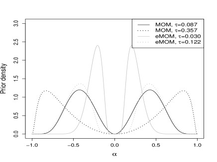
To set ( under ) we reparameterize as in Rubio and Steel (2014). These authors proposed , which places the prior mode at and thus defines a local prior. Our goal here is to detect situations where the degree of asymmetry is practically relevant and to otherwise allow the posterior to collapse on the symmetric model. To achieve this, we consider , and , where is a fixed prior dispersion parameter. To set , by default we consider that Arnold-Groeneveld asymmetry coefficients are often practically irrelevant. Thus, we set such that . Also, note that gives a total variation distance of , i.e. the largest difference for any set is 0.1, which we typically view as irrelevant. Since , a direct calculation gives that when under MOM and eMOM. To assess sensitivity in our examples, we also considered such that (total variation distance=0.05), giving . Figure 1 depicts under these settings. Our results showed that variable selection is typically robust to choices of within this range.
 |
4. Parameter estimation
We obtain some results for parameter estimation under a given that are also useful to establish variable selection rates (see Section 5 for results on Bayesian model averaging). Section 4.1 gives the limiting distribution of as for asymmetric Normal and Laplace when data are generated from (1) but the error model may be misspecified. Briefly, as is typically the case, we obtain parameter estimation consistency and asymptotic normality, albeit there is a loss of efficiency and an underestimation of uncertainty. Section 4.2 presents novel optimization algorithms for maximum likelihood and posterior mode estimation designed to improve the computational scalability of current related methods.
4.1. Asymptotic distributions
We lay out technical conditions for our asymptotic results to hold.
-
A1.
The parameter space is compact and convex.
-
A2.
Data are truly generated as for some , fixed and are i.i.d. and independent of . Let the data-generating with density for all .
-
A3.
For all there is some such that is strictly positive definite almost surely for all .
-
A4.
Denote by the generating process of the covariates (which can be either stochastic or deterministic).
where , and we specify the order of interest in each of the results below, and denotes the Euclidean distance .
-
A5.
For
These conditions are in line with those in classical robust regression, e.g. see Huber (1973) or Koenker and Bassett (1982). Condition A1 is made out of technical convenience, naturally one may take an arbitrarily large . Condition A2 states that data truly arise from a linear model, where the key assumption is that the residuals are independent. Extensions to non-id errors are discussed in Section 5.2. Condition A3 holds whenever the rows of are regarded as a deterministic sequence satisfying the condition, or for instance when are independent and identically distributed from an underlying distribution of fixed dimension with positive-definite , as then converges almost surely to a positive-definite matrix by the strong law of large numbers. We focus on fixed , extensions to growing with are possible along the lines in Mendelson (2014), but its detailed treatment is beyond the scope of this paper. Condition A4 requires existence of moments up to a certain order. Condition A5 requires being able to exchange integration and differentiation, and is needed only to prove asymptotic normality.
Our results summarize and extend classical studies focusing on in least squares, median and quantile regression to consider the whole parameter vector . Briefly, Eicker (1964) and Srivastava (1971) showed that the least squares estimator () satisfies , where minimizes Kullback-Leibler divergence to the data-generating truth and , assuming that and minimum conditions on . To our knowledge, the asymmetric Normal has been much less studied, e.g. Kimber (1985), Mudholkar and Hutson (2000) and Arellano-Valle et al. (2005) considered the case with no covariates and no checks of the conditions required by large sample theory are shown, which are non-trivial given that is discontinuous. Regarding Laplace errors (), Pollard (1991) and Knight (1999) showed , where and is the median of , under mild conditions on and . Koenker (1994) generalized the result to the asymmetric Laplace, obtaining , where evaluated at the quantile , where in our parameterization . Proposition 3 establishes the consistency of the maximum likelihood estimator to the Kullback-Leibler optimal parameter values, whereas Proposition 4 gives asymptotic normality.
Proposition 3.
Assume Conditions A1–A4 with , where in A4 when and when . Then, the function has a unique maximizer . Moreover, the maximum likelihood estimator as .
Proposition 4.
Assume Conditions A1–A5, with in A4 when and when . Denote , , , and . Then, the sequence is asymptotically Normal with mean and covariance matrix , where is the gradient of , with respect to , evaluated at and is the second derivative matrix of evaluated at .
The sandwich covariance is typically an inflated version of that obtained when the true model is assumed (), implying the well-known consequence of model misspecification that parameter estimation suffers a loss of efficiency and uncertainty is underestimated. To gain insight, Corollary 1 gives specific asymptotic variances under various model misspecification cases. For instance, when truly wrongly assuming Laplace errors increases the variance by a factor , and a similar phenomenon is observed when ignoring the presence of residual asymmetry. We defer discussion of the implications for variable selection to Section 5 and the examples in Section 6.
Corollary 1.
The asymptotic distribution of obtained by maximizing either the Normal, ANormal, Laplace or ALaplace likelihood is , for some . The asymptotic variances , when truly arise i.i.d. under four specific distributions, are given below.
| Maximized log-likelihood | ||||
|---|---|---|---|---|
| True model | Normal | ANormal | Laplace | ALaplace |
| () | ||||
where , , and is as in Proposition 4. Cases marked were derived assuming that covariates have zero mean.
4.2. Optimization
We outline simple, efficient algorithms to obtain , where are the asymmetric Normal and Laplace log-likelihoods (3)-(4). We also consider the corresponding posterior modes , where is the prior density (Section 3). The algorithms are useful to obtain parameter estimates or Laplace approximations to the integrated likelihood. Mudholkar and Hutson (2000) and Arellano-Valle et al. (2005) gave an algorithm to obtain for in the case with no covariates (). To tackle point discontinuities in the derivatives their algorithm requires solving separate optimization problems, which does not scale up with increasing , or alternatively using method of moments estimators. Maximum likelihood estimation of under the asymmetric Laplace and fixed is connected to quantile regression (see below). Regarding Bayesian frameworks, most rely on MCMC for parameter estimation but this is too costly when we wish to consider a potentially large number of models. Instead, we propose a generic framework for jointly obtaining or applicable to both the asymmetric Normal and Laplace. The key result we exploit is concavity of the log-likelihood given by Propositions 1-2, which allows iteratively optimizing first and then . Optimization with respect to has closed form, whereas setting can be seen as weighted least squares for the asymmetric Normal and as quantile regression for the asymmetric Laplace. The latter task of maximizing with respect to is a classical problem that can be framed as linear programming, for which simplex and interior-point methods are available. However, these are not applicable to the posterior mode as the target is no longer piecewise linear and even efficient implementations have computational complexity greater than cubic in and supra-linear in Koenker (2005).
We outline two simple algorithms that have lower complexity and can be readily adapted to obtain the posterior mode. Briefly, in Algorithm 4.2, Step 2 follows from setting first derivatives to zero and directly extends Mudholkar and Hutson (2000) (Proposition 4.4) and Arellano-Valle et al. (2005) (Section 4.2). Step 3 is essentially a Levenberg-Marquardt algorithm Levenberg (1944); Marquardt (1963) exploiting gradient continuity. and denote the gradient and hessian with respect to as in Propositions 1-2, where for we use the asymptotic hessian . Its updates are in between those of a Newton-Raphson and gradient descent algorithms and can be interpreted as restricting the Newton-Raphson step to a trust region where the quadratic approximation is accurate Sorensen (1982). For large regularization parameter the update converges to the gradient algorithm, which by continuity is guaranteed to increase the target, whereas for small it converges to the Newton-Raphson algorithm, achieving quadratic convergence as approaches the optimum.
Optimization via Levenberg-Marquardt
-
(1)
Initialize , . Set
-
(2)
Let , . Update
-
(3)
Propose , where
and are the subsets of and corresponding to . If set and , else update and repeat Step 3.
Given a good initial guess , the fact that are locally well approximated by a quadratic function in ( is exactly locally quadratic) results in Algorithm 4.2 usually converging after a few iterations. As usual, with second-order optimization each iteration requires a matrix inversion that is costly when is large. As an alternative, Algorithm 4.2 uses coordinate descent to optimize each sequentially, which only requires univariate updates, where updating the set for each implies that Step 3 has cost . In contrast, Algorithm 4.2 determines once per iteration and performs matrix inversion, with total cost per iteration. Hence, although Algorithm 4.2 usually requires fewer iterations than Algorithm 4.2, for large the latter is typically preferrable. A related study of computational cost is offered in Breheny and Huang (2011) in the context of penalized likelihood optimization, who found that coordinate descent is often preferrable to multivariate updates. These results show that, contrary to historical beliefs, two-piece distributions lead to convenient optimization. R package mombf Rossell et al. (2016) incorporates both algorithms but our examples are based on Algorithm 4.2, the results were essentially identical to those of Algorithm 4.2 but the running time was substantially shorter.
We adapted both algorithms to find the posterior mode by simply redefining and to be the gradient and Hessian of . The corresponding expressions are in Supplementary Section 10.2. We remark that due to the penalty around the origin NLPs such as and in (6)-(7) are not log-concave, however this is not an issue as they are symmetric and log-concave in each quadrant (fixed ). Thus is concave in each quadrant, its unique global mode lies in the same quadrant as the maximum likelihood estimator and we may initialize the algorithm at . Convergence is typically achieved after a few iterations.
5. Model selection
Under a standard Bayesian framework , with integrated likelihood
| (8) |
Section 5.1 discusses how to compute and Section 5.2 the asymptotic properties of the associated Bayes factors and Bayesian model averaging, along with a discussion on model misspecification and to what extent these results can be generalized to non-identically distributed errors (e.g. under heteroscedasticity or hetero-asymmetry). Section 5.3 outlines a stochastic model search algorithm that can be used when is too large for exhaustive enumeration of the models.
5.1. Integrated likelihood
Computing (8) in the case corresponds to Normal linear regression, for which existing methods are typically available, e.g. Johnson and Rossell (2012) gave closed-form expressions for the MOM and Laplace approximations for the eMOM. The three remaining cases require numerical evaluation, for which we propose Laplace and Monte Carlo approximations. The former are appealing due to log-likelihood concavity and asymptotic normality (Section 4). Indeed, in our examples they delivered very similar inference and were orders of magnitude faster than Monte Carlo. Hence, by default we recommend Laplace approximations over Monte Carlo, except in small situations where the latter is still practical. To ensure that the parameter support is on the real numbers Laplace approximations are based on the reparameterization and given by
| (9) |
where for respectively, and are the posterior mode and hessian of . The specific expressions are given in Supplementary Section 10. Expression (9) simply requires the posterior mode (Algorithms 4.2-4.2) and evaluating the hessian. The latter is straightforward for , but for it is singular in , requiring some care. The reasoning behind (9) is to approximate the log-integrand in (8) by a smooth function that has strictly positive definite hessian in , which is facilitated in our setting by concavity and asymptotic normality. We found that a simple yet effective strategy is to replace by the asymptotic expected hessian obtained under independent asymmetric Laplace errors.
Although we did not find the following concern to be a practical issue in our examples, we remark that in principle may underestimate the underlying uncertainty in and thus inflate , e.g. under truly non-Laplacian independent and identically distributed errors one needs to add a multiplicative constant (Section 4.1), whereas independent but heteroscedastic errors require a matrix-reweighting adjustment Kocherginsky et al. (2005). Typical strategies to improve the estimated curvature rely either on direct estimation under the assumption of independent and identically distributed errors, or indirect estimation via inversion of score tests, although these only provide univariate confidence intervals and their cost does not scale well with , or sampling-based methods such as bootstrap or Monte Carlo. As a practical alternative here we consider that the goal is really to approximate the actual curvature of , which can be easily done with a few point evaluations of in a neighbourhood of . Briefly, we consider the adjustment , where is a diagonal matrix such that its element gives the best approximation of as a quadratic function of in the least squares sense. matches the actual curvature in and is thus less dependent on asymptotic theory than other strategies, and has the advantage that can be computed quickly. See Supplementary Section 10.3 for further details and Supplementary Figure 6 for an example. Given that the unadjusted performed well in our examples and the associated results were practically indistinguishable to those based on Monte Carlo, unless otherwise stated our results are based on .
As our Monte Carlo alternative, we implemented an importance sampling estimator based on multivariate T draws and covariance matching the asymptotic posterior covariance. Specifically, let for where is a large integer, then
| (10) |
We remark that NLPs are multimodal in , thus some care is needed when using Laplace approximations. To give an honest characterization of the properties of our preferred computational method, in Section 5 we obtain asymptotic rates for Bayes factors based on in (9). Rossell and Telesca (2017) studied the discrepancies between and for MOM, iMOM and eMOM priors and Normal errors. Briefly, given that secondary modes vanish asymptotically for truly active covariates but not for spurious covariates, imposes a stronger penalty on spurious variables than , however for such models decreases fast enough that both approximations typically lead to very similar inference.
5.2. Bayes factor rates
Let be the optimal model, that is maximize the expected log-likelihood across , and the expectation is with respect to the data-generating density in Condition A1. We indicate by that is a submodel of , i.e. for , and by that for some . If the data were truly generated from the assumed error distribution, it is well-known that the Bayes factor in favour of decreases exponentially with when ( is missing important variables). Conversely when adds spurious variables to the Bayes factor is only under local priors, an imbalance that is ameliorated under NLPs, which achieve faster polynomial or quasi-exponential rates depending on their chosen parametric form Johnson and Rossell (2010, 2012). Proposition 5 gives an extension under model misspecification, the first result of this kind for NLPs. We remark that the rates apply directly to the Laplace approximations (9). As studied by Rossell and Telesca (2017) (Supplementary Section 5, Supplementary Figure 8), when contains spurious parameters the non-local posterior can have non-vanishing multimodality, in which case Laplace approximations underestimate even as . In our experience this is not a major concern (e.g. Table 3S compares Laplace with importance sampling estimates), but we find it preferrable to characterize inference under our recommended computational framework, i.e. for . A critical condition for Proposition 5 is that the prior density be strictly positive at the optimum, , which is trivially satisfied by pMOM and peMOM priors. It also holds for local priors, which for simplicity we define as for all and we assume to be continuous.
Proposition 5.
Suppose that Conditions A1-A3 hold, fixed and . If then for local, pMOM and peMOM priors and some constant . Conversely, if then where for local priors, for the pMOM prior, and for the peMOM prior where .
Corollary 2.
Let be Bayesian model averaging estimates, , , where is non-increasing in and . Under the conditions in Proposition 5, if then under the pMOM prior and under the peMOM prior. If then under the pMOM and peMOM priors.
Proposition 5 implies model selection consistency with Bayes factor rates that have the same functional form as when the correct model is assumed. We emphasize that this does not imply that there is no cost due to assuming an incorrect model: the coefficient in the exponential or those in the polynomial rates are affected. The constant determines how quickly one can detect truly active variables (asymptotically) and is given by the KL divergence between the assumed model class and the data-generating truth. That is, under the true model takes a different value than under a misspecified model and hence the ratio of the correct versus misspecified Bayes factors to detect signals is essentially exponential in . In contrast, when this ratio converges to a constant, hence the effects of model misspecification on false positives vanishes asymptotically. We remark that, for finite , misspecification can have a marked effect on false positives, see Section 6.2 for examples. Corollary 2 is the trivial implication that Bayes factors also drive parameter estimation shrinkage in a Bayesian model averaging setting Rossell and Telesca (2017). When , the shrinkage is or for pMOM and peMOM respectively, in contrast to for local priors and for the unregularized MLE, times a term given by model prior probabilities.
We remark that Conditions A1-A3 for Proposition 5 assume independent and identically distributed (id) errors. It is possible to relax these conditions, particularly that of id errors. Loosely speaking, the three main ingredients in the proof are that (MLE consistency), that asymptotically for some constants , and that the likelihood ratio statistic between and a supra-model is bounded in probability. The MLE and likelihood ratio conditions hold quite generally for non-id errors, in particular the latter is satisfied whenever its limiting distribution is say a chi-square or mixture of chi-squares. Regarding , under independent but non-id errors the ALaplace model has where is a constant depending on and an diagonal matrix accounting for each observation’s variance Kocherginsky et al. (2005). The Laplace model is a particular case of this result. Under Normal errors the MLE has the non-asymptotic covariance , and similarly for the asymmetric least squares criterion implied by the two-piece Normal. Provided that is bounded or grows at a slower-than-polynomial rate with and the eigenvalues of lie between two positive constants, then for some . Relaxing the independence assumption requires more care, e.g. under very strong dependence could grow at a slower rate than . We remark that these observations are simply meant to provide intuition, obtaining precise conditions for Proposition 5 under non-iid settings is an interesting question for future research.
From the discussion above model misspecification affects sensitivity via the constant . In our experience, typically there is a loss of power. Fully characterizing this issue theoretically is complicated as depends on the unknown data-generating truth, but it is possible to provide some intuition. Consider an arbitrary variable configuration that is missing some truly active variables. Suppose that, as in Condition A1, truly for some error density family , , and fixed . Denote by the likelihood under the correct and the associated integrated likelihood under some prior . The interest is in comparing the correct Bayes factor to the misspecified . Under fairly general conditions
plus lower order terms analogous to those in Proposition 5 when , where is the Kullback-Leibler divergence between the data-generating and the KL-optimal under . Trivial algebra gives
| (11) |
The sign of the right hand side in (11) determines whether the misspecified Bayes factor has lower or greater asymptotic power than the correct Bayes factor. A precise study of (11) deserves separate treatment, but the expression can be loosely interpreted as a type of triangle inequality. If the divergence due to simultaneously using the wrong error distribution and instead of , , is smaller than the sum of the divergences due to only using the wrong error distribution plus that of only using instead of . Then, misspecifiying the error distribution results in slower (but still exponential) Bayes factor rates to detect truly active variables. To our knowledge there is no guarantee that (11) is positive in general for any assumed model and data-generating truth, however in all our examples misspecified Bayes factors exhibited such a loss of power, suggesting that this is often the case.
5.3. Model exploration
Algorithm 5.3 describes a novel Gibbs sampling that can be used when is too large for exhaustive enumeration of all models. Although conceptually simple, Algorithm 5.3 extends a method that delivered good results for high-dimensional variable selection under Normal errors Johnson and Rossell (2012), and is designed to spend most iterations in the Normal model whenever it is a good enough approximation. That is, as illustrated in our examples the computational effort adapts automatically to the nature of the data, so that the cost associated to abandoning the Normal model is only incurred when this is required to improve inference. Our implementation also allows the user to fix , so that one can condition on Normal, asymmetric Normal, Laplace or asymmetric Laplace errors whenever this is desired.
The number of iterations should ideally be large enough for the chain to converge, see for instance Johnson (2013) for a discussion of formal convergence diagnostics based on coupling methods. In practice, it usually suffices to monitor some posterior quantities of interest. For instance, in the setting of variable selection with NLPs Rossell and Telesca (2017) found useful to set large enough so that sampling-based estimates of are close enough to estimates based on renormalizing posterior probabilities across the models visited so far.
Gibbs model space search.
-
(1)
Let and set using the greedy forward-backward initialization algorithm in Johnson and Rossell (2012). Set .
-
(2)
For , update with probability
-
(3)
Update with probability
If , set and go back to Step 2, otherwise stop.
6. Results
We studied via simulations the practical implications of model misspecification on variable selection, both on small and large (Sections 6.1-6.3), as well as the ability of our framework to detect asymmetries () and heavier-than-normal tails (). The heteroscedastic errors simulation in Section 6.2 and the DLD example in Section 6.5 also illustrates how to perform quantile regression for multiple fixed quantile levels as a particular case of our framework.
Computations were carried out using function modelSelection in R package mombf 1.9.2 Rossell et al. (2016), using default prior settings (Section 3) and Laplace approximations to unless otherwise stated. Although our goal is to build a Bayesian framework to cope with simple departures from normality, for comparison we included some penalized likelihood methods with available R implementation: standard LASSO penalties on least squares regression (LASSO-LS, Tibshirani (1996)), LASSO penalties on least absolute deviation (LASSO-LAD, Wang and Li (2009)), SCAD penalties on least squares Fan and Li (2001), and LASSO penalties on quantile regression (LASSO-QR, Wu and Liu (2009)). For LASSO-LS, LASSO-LAD, LASSO-QR and SCAD we set the penalization parameter with 10-fold cross-validation using functions mylars, rq.lasso.fit and ncvreg in R packages parcor 0.2.6, rqPen 1.5.1 and ncvreg 3.4.0 (respectively) with default parameters. LASSO-LAD corresponds to setting the 0.5 quantile in rq.lasso.fit, whereas for LASSO-QR we set the optimal quantile where is the data-generating truth. That is, we performed a conservative comparison where results for LASSO-QR may be slightly optimistic. All R code is provided in supplementary files.
6.1. Low-dimensional simulation
| Normal | ANormal |
 |
 |
| Laplace | ALaplace |
 |
 |
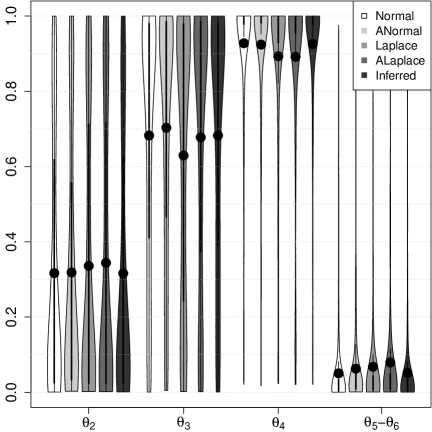
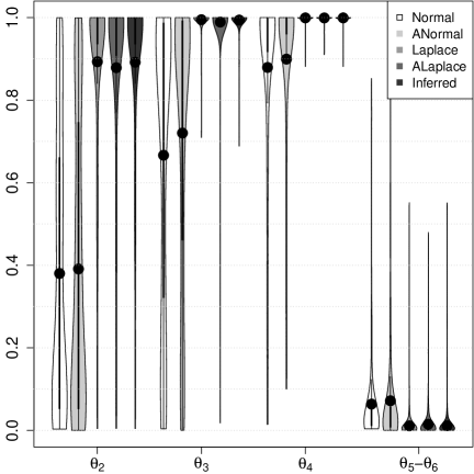
We started by simulating 200 data sets from a linear model with Normal residuals, each with , , ( corresponds to the intercept), . Covariate values were generated from a multivariate Normal centered at 0, with unit variances and all pairwise correlations . We compared the results under assumed Normal, asymmetric Normal, Laplace and asymmetric Laplace errors, and also when inferring the residual distribution with our framework (Section 5). Throughout, we used MOM priors with default , and uniform model probabilities . Given that is small we enumerated and computed for all models. Figure 2 (top left) shows the marginal posterior probabilities . These were almost identical under assumed Normal and asymmetric Normal errors. Both models were preferrable to Laplace or asymmetric Laplace errors, mainly in giving higher for truly active variables.
We repeated the simulation study, this time generating , and finally . Here we observed more marked differences than under , specifically failing to account for thick tails caused a substantial drop in for truly active predictors. As an example, when truly the mean increased from 0.63 under assumed Normal errors to 0.89 under asymmetric Laplace errors. These results suggest that wrongly assuming Normal errors may has more pronounced consequences on inference than using more robust error distributions. Interestingly, including asymmetry in the model had no noticeable adverse effects on inference even when residuals were truly symmetric, and improved power when residuals were truly asymmetric. Hence the reasoning for adopting symmetric models seems mostly computational.
Our framework based on inferring showed a highly competitive behaviour, usually fairly close to assuming the true distribution (Figure 2). The mean posterior probability assigned to the true error distribution was always (Supplementary Table 4), indicating that the desired departures from normality were effectively detected.
We repeated all the analyses above first using Monte Carlo estimates of based on importance samples, and then again using our alternative default . Supplementary Table 4 shows that inference on the error distribution remained remarkably stable, albeit as expected reducing to increases slightly in all settings. Supplementary Figures 7-8 show . These are virtually indistinguishable from those in Figure 2, indicating that the results are robust to these implementation details.
Finally, we assessed the behaviour of the least-squares initialization in Algorithms 4.2-4.2 under different data-generating mechanisms, specifically in terms of CPU times. Table 2 gives mean times across independent simulations with and increasing data-generating truths , both for two-piece Normal and two-piece Laplace errors. These are for the whole model-fitting process, including exhaustive model enumeration and computation of posterior model probabilities. The time increases were of roughly 25% from to . This is as expected, under asymmetry least-squares is a poorer initial . The increase is however mild, indicating that a larger fraction of the computation cost arises from other operations (e.g. matrix inversion after the mode has been found). These results support that our is not particularly problematic. One could certainly consider alternative , say median regression or trimmed least squares, but these are typically costlier that least-squares hence the overall gains are likely to be moderate at best.
6.2. Non-identically distributed errors
| Normal | ANormal |
 |
 |
| Laplace | ALaplace |
 |
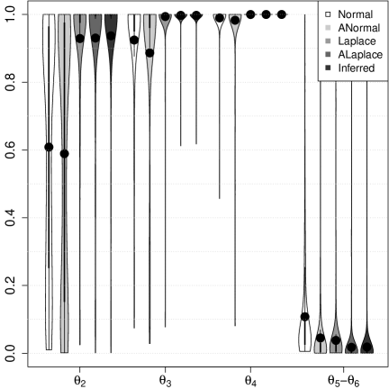 |
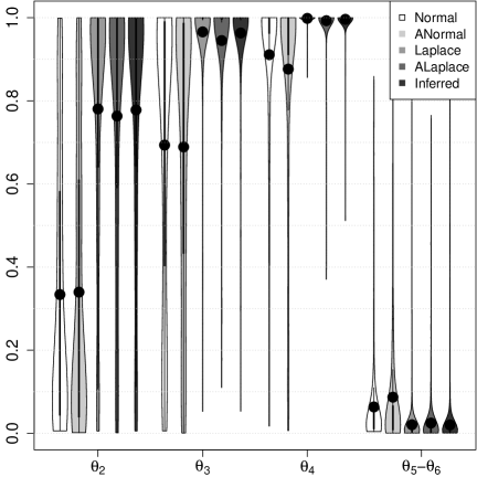
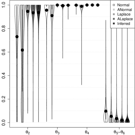
We investigate the effect of deviations from the identically distributed errors assumption. We repeated the simulations in Section 6.1 under heteroscedastic and hetero-asymmetric errors, and reproduced a pathological example reported by Grünwald and van Ommen (2014). Under heteroscedasticity, we set where was set such that , so that the signal-to-noise was comparable to our earlier simulations. This example mimics that used by Koenker (2005) (Figure 1.6) to illustrate the potential interest of conditioning upon multiple quantile levels, except that ours has a stronger (exponential) association between mean and variance. We first apply our framework without conditioning on . Figure 3 shows for . The main feature is that the Laplace and asymmetric Laplace models clearly outperform the Normal model both in sensitivity and specificity. For instance, when truly the mean increased from 0.33 to 0.78 under assumed Normal and Laplace residuals respectively. The mean for truly inactive decreased from 0.063 to 0.021. Interestingly, inferring the error model chose Laplace errors even when these were truly Normal and showed a highly competitive performance (Supplementary Table 8). Intuitively, heteroscedasticity gives an overabundance of residuals at the origin and at the tails relative to a homoscedastic Normal. Such errors are better captured by a Laplace model.
Next, following Koenker (2005) we assessed the performance of quantile regression at fixed quantile levels . The usual motivation for conditioning upon multiple quantiles is to consider that each quantile could potentially depend on a different subset of predictors. This corresponds to conditioning upon asymmetric Laplace errors and fixed (Section 2). The marginal posterior inclusion probabilities in Table 9 show that (the KL-optimal value) led to substantially higher sensitivity than say or . We remark that under our heteroscedastic data-generating truth the conditional quantile is where is the standard Normal quantile. The results illustrate that, in this and similar situations where all quantiles depend on the same subset of variables, inferring can lead to better variable selection than conditioning upon poor choices of . Naturally, under more complex scenarios where quantiles do depend on different variable subsets, conditioning upon multiple can provide a richer description of the dependence of on .
Our second simulation scenario considered the presence of non-constant asymmetry. Specifically, we generated where the median asymmetry is as before. Under this setting when then with 0.95 probability and when it is , i.e. there is substantial variation in asymmetry. Supplementary Figure 13 displays for . These results are qualitatively similar to those in Figure 2 where was held fixed. We remark that although in these examples non-constant asymmetry was not a concern, its impact could be more serious in other settings, e.g. under strong dependencies between the asymmetry and the mean. See Section 7 for some further discussion.
Finally, we mimic the example in Grünwald and van Ommen (2014), Section 5.1.2. The authors set with probability 0.5 and with probability 0.5, where , and . This extreme case of non-id errors is interesting in that the degeneracy at the origin results in inliers, rather than the more commonly considered outliers in or leverage points in . We selected variables under assumed Normal errors for , for this the authors reported a particularly large inflation of false positives (as these disappeared). Specifically we set , Zellner’s and the Beta-Binomial(1,1) prior for . The posterior mode selected a striking 21.3 out of the 45 spurious variables (mean across 100 independent simulations), confirming their findings (Supplementary Table 10). Under a pMOM prior the mean false positives decreased to 12.1 when conditioning on Normal errors and further to 10.5 when inferring the error model. Interestingly under the peMOM prior and Normal errors the mean false positives were only 2.9. All methods showed similar sensitivity, selecting roughly 3 out of the 5 active variables. This example illustrates that, while serious model misspecification can have marked effects for finite , these can be partially mitigated by adopting priors that penalize small coefficients and flexible error models. In this particular example the exponential peMOM penalties were more effective than the pMOM penalties in lowering false positives.
6.3. High dimensional simulation
 |
 |
 |
 |
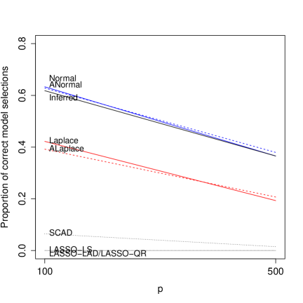
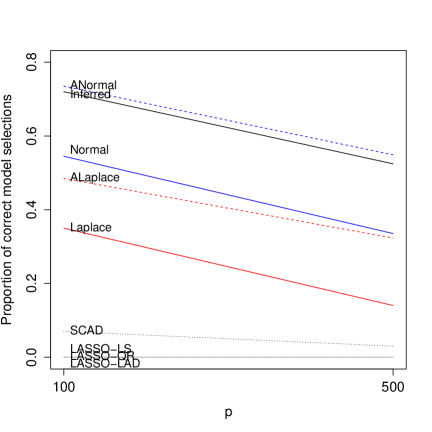
We repeated the simulation study in Section 6.1 with by adding 95 spurious predictors for a total of covariates, and subsequently 400 more spurious predictors for a total . Given that the model space is too large for a full enumeration, we run the Gibbs algorithm in Section 5.3 with iterations. To initialize the chain we used the greedy Gibbs algorithm from Johnson and Rossell (2012), which starts at and keeps adding or removing individual covariates until a local mode is found. We set to the default Beta-Binomial(1,1) and left all other settings as in Section 6.1.
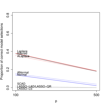
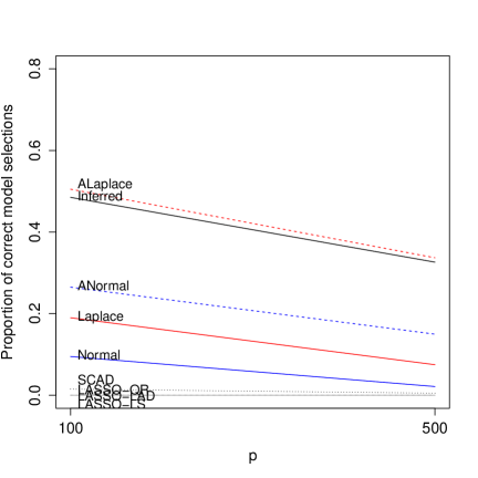
We conducted one first set of simulations under . Figure 4 shows the proportion of simulations in which the posterior mode was equal to the simulation truth . The main finding was that assuming the wrong error distribution had a marked detrimental impact on Bayesian variable selection, particularly in the presence of asymmetries or thicker-than-normal tails. Supplementary Table 6 gives the exact figures, as well as the number of false and true positives. All Bayesian formulations compared favourably to LASSO-LS, LASSO-LAD, LASSO-QR and LASSO-SCAD, mainly due to the latter incurring an inflated number of false positives. This is in agreement with earlier findings Johnson and Rossell (2012); Rossell and Telesca (2017) when comparing NLPs to penalized likelihoods, and likely partially related to the fact that cross-validation focuses on predictive ability and thus tends to favour the inclusion of a few spurious covariates. Interestingly, in our study LASSO-LAD showed little advantages over LASSO-LS, even under truly Laplace errors. LASSO-QR did improve slightly upon LASSO-SCAD when truly both in sensitivity and specificity. Analogously to the case in Figure 2, when the marginal inclusion probabilities for truly active variables suffered a drop when ignoring the presence of asymmetry or heavy tails (Supplementary Figures 9-10). Our framework to infer the error distribution delivered highly competitive inference.
Supplementary Table 3 indicates CPU times for . The Normal model exhibited lower times under truly Normal or Laplace errors, likely due to the availability of closed-form expressions for . The presence of asymmetry encouraged the inclusion of an intercept term under the Normal model, the associated increase in model dimension cancelled the computational savings. Times for our inferred residuals framework were highly competitive under all scenarios.
To emulate a situation with lower signal-to-noise ratio we repeated the simulation study under . The results are shown in Supplementary Table 7 and Supplementary Figures 11-12. Briefly, the performance of all methods suffered in this more challenging setting due to a drop in the power to detect truly active predictors, however their relative performances were largely analogous to those for .
6.4. TGFB data
 |
 |
We illustrate our methodology with the human microarray gene expression data in colon cancer patients from Calon et al. (2012). Briefly, following upon Rossell and Telesca (2017), we aim to detect which amongst 10,172 candidate genes have an effect on the expression levels of TGFB, a gene known to play an important role in colon cancer progression. These data contain moderately correlated covariates with absolute Pearson correlations ranging in (0,0.956) and 99% of them being in the interval (0,0.375). Both response and predictors were standardized to zero mean and unit variance. The dataset and further information are provided in Rossell and Telesca (2017).
| Gene symbol | ||
|---|---|---|
| Normal | Inferred | |
| ARL4C,AOC3,URB2,FAM89B,PCGF2,CCDC102B | 0.299 | 0.304 |
| ARL4C,CNRIP1,AOC3,PCGF2 | 0.165 | 0.167 |
| ARL4C,CNRIP1,PCGF2 | 0.161 | 0.163 |
| ARL4C,CNRIP1,AOC3,PCGF2,RPS6KB2 | 0.045 | 0.046 |
| ARL4C,AOC3,PCGF2,CCDC102B | 0.028 | 0.028 |
| ARL4C,AOC3,FAM89B,PCGF2,CCDC102B | 0.025 | 0.025 |
We start by considering inference under the Normal model, i.e. conditional on . We ran 1,000 Gibbs iterations (i.e. model updates), which was deemed sufficient for practical convergence (see supplementary material in Rossell and Telesca (2017)). Table 1 shows the highest posterior probability models. The top model included the 6 genes ARL4C, AOC3, URB2, FAM89B, PCGF2, CCDC102B and had an estimated . Alternatively, selecting variables with marginal Barbieri and Berger (2004) returned 5 out of these 6 genes ( for FAM89B). Briefly, according to genecards.org FAM89B is a TGFB regulator, ARL4C and PCGF2 have been related to various cancer types and AOC3 is used to alleviate cancer symptoms, reinforcing the plausibility that these genes may be indeed related to TGFB. URB2 and CCDC102B have no known relation to cancer, although the latter is connected to ARL4D in the STRING interaction networks.
We next considered the possibility that the Normal model might not be adequate for these data. As an exploratory check, a quantile-quantile plot based on the residuals under the top model revealed no strong departure from normality (Figure 5). Although this is somewhat reassuring one cannot discard a lack of normality under a different set of predictors, as the top model was selected under assumed normality. To conduct a more formal analysis we run Algorithm 5.3 ( iterations) now including . The posterior probabilities for Normal, asymmetric Normal, Laplace and asymmetric Laplace errors were 0.998, 0.0002, 0.0018 and 1.3, respectively. The six top models and their posterior probabilities closely matched those under the assumed Normal model (Table 1), and the correlation between marginal inclusion probabilities under Normal and inferred residuals was 0.96. These results support that our framework to infer in Algorithm 5.3 is able to detect when errors are approximately Normal.
6.5. DLD data
We consider another genomics study by Yuan et al. (2016). In contrast to Section 6.4, here RNA-sequencing was used to measure gene expression, a newer and more precise technology than microarrays. The study included 100 colorectal, 36 prostate, and 6 pancreatic cancer and 50 healthy control patients, for a total of patients. Briefly, the authors used a measure of expression called RPM. RPM considers the number of reads mapped to a given gene relative to the gene length and may exhibit heavy tails or asymmetries, even after log or other transformations. We focus on the 58 messenger RNA genes identified in the exRNA species diversity analysis provided by the authors in Supplementary Table S1. To illustrate our methodology, we consider predicting the expression of gene DLD based on the remaining 57 genes and the 3 binary variables indicating the patient type (colorectal, prostate, pancreatic). According to genecards.org, the protein encoded by DLD can perform mechanistically distinct functions, it can regulate the energy metabolism and has been found to be associated with dehydrogenase and leukocyte adhesion defficiencies.
We first applied our methodology conditioning on Normal errors (). We used 10,000 Gibbs iterations. The highest posterior probability model had and contained 5 genes (C6orf226, ECH1, CSF2RA, FBXL19, RRP1B), however, its residuals showed a clear departure from normality (Figure 5, right). We run again our Gibbs algorithm, this time inferring and . The analysis returned an overwhelming in favour of Laplace residuals. The top model had posterior probability 0.36 and contained the same 5 predictors plus an extra gene MTMR1. MTMR1 encodes a protein related to the myotubularin family containing consensus sequences for protein tyrase phosphatases, whereas the response gene DLD has a post-translational modification based on tyrosine phosphorylation, thus giving a plausible biological mechanism connecting MTMR1 and DLD. Supplementary Table 11 lists the six largest marginal variable inclusion probabilities under Normal and inferred error distribution.
So far, we treated as a parameter to be learnt from the data. We now condition upon asymmetric Laplace errors and fixed . This leads to quantile regression for the percentiles (Section 2). Supplementary Table 12 displays the top 5 models for each . Briefly, five genes (C6orf226, CSF2RA, ECH1, RRP1B and FBXL19) featured in the top model for all ’s, the first four with marginal inclusion probability . FBXL19 had higher probability under than (0.783 vs. 0.516 and 0.467 respectively). MTMR1 featured in the top model only for (marginal probability 0.619). Given the biological plausibility that MTMR1 is related to DLD, these results suggest that setting (the value inferred from the data) may have led to higher power to detect MTMR1 than conditioning on Normal or asymmetric Laplace residuals with or . This is in agreement with Proposition 5 and our simulations in Sections 6.1-6.3.
7. Discussion
Most efforts in Bayesian variable selection focus either on the Normal model or on flexible alternatives that require MCMC. Our framework represents a middle-ground to add flexibility in a parsimonious manner that remains analytically and computationally tractable, facilitating applications where either is large or is too moderate to fit more complex models accurately. Our results show that model misspecification is a non-ignorable issue with important consequences for model selection. Bayes factor rates typically retain the same functional dependence on (e.g. polynomial or exponential) as when the model is correctly specified, however the coefficients governing these rates do change. Specifically, the ratio of the correct vs. misspecified Bayes factors to detect truly active variables grows exponentially with when a triangle-type inequality holds, signaling the potential for an important drop in sensitivity. Our empirical studies support this finding: failing to account for simple forms of asymmetry or heavy tails reduced the proportion of correct model selections by several folds. Misspecification also has an effect on false positives. Although here the ratio of correct vs. misspecified Bayes factors is essentially a constant, the effect can be noticeable for finite . Hence it is important to consider flexible likelihoods and, when possible, also adopt false positive correction mechanisms for finite . As a possible venue for the latter, we illustrated in an example how non-local priors helped discard small spurious parameters arising from misspecification. A more detailed study would be interesting future work.
Other future avenues include extensions to allow for polynomial error tails, dependent errors, heteroscedasticity or covariate-dependent asymmetry. We remark that fully non-parametric strategies already exist, e.g. Chung and Dunson (2009). The challenge is to build models that provide an intermediate level of flexibility while giving tractable variable selection. For instance, allowing the variance or asymmetry to depend on is an interesting task for which there is no unique agreed-upon solution. One possibility is to let , where , akin to what Daye et al. (2012) for Normal errors. The authors found that the log-likelihood for for fixed is log-concave, and so is that for under fixed , enabling fast optimization. It would be interesting to develop similar strategies for the asymmetry and non-Normal errors. An issue here would be dealing with the increased problem dimensionality due to selecting variables also for . Another interesting venue stemming from our work is posing non-parametric models that can collapse onto simple parametric forms when the extra flexibility is not needed. Again the idea is to strike a balance between the tractability offered by simple models and the ultimate goal of providing accurate inference. Other extensions are developing more advanced optimization or model search strategies, our goal here was to illustrate that even relatively simple methods can be competitive. Such computational issues are particularly meaningful in increasingly challenging settings, e.g. large graphical or spatio-temporal models. Overall, we hope to have provided a basic framework that others can build on to tackle these exciting applications.
Supplementary material. Tractable Bayesian variable selection: beyond normality
8. iMOM prior
The product iMOM prior density on Johnson and Rossell (2012) is given by
| (12) |
where by default assigns . Regarding the asymmetry parameter , the prior is , and the default prior dispersions are to obtain and for .
9. Proofs
For simplicity, we drop from the notation in the proof of Propositions 1-4 and Corollay 1, given that all arguments are conditional on a given model .
9.1. Proof of Proposition 1
We start by stating a useful lemma stating that positive definite hessian plus continuous gradient guarantees concavity.
Lemma 6.
Let be a function with continuous gradient , for all , and negative definite hessian almost everywhere with respect to the Lebesgue measure. Then, is strictly concave. If is negative semidefinite, then is concave.
Proof.
Let and be two arbitrary values and denote where . Define , to show that is concave it suffices to see that is convex for arbitrary . Straightforward algebra shows that and further derivation shows that
since is negative definite ( for negative semidefinite).
The second derivative almost everywhere and the first derivative is continuous, which implies that is strictly increasing in and hence is strictly convex (non-strictly convex when is negative semidefinite). ∎
Proof of Proposition 1, Part (i)
The gradient follows from straightforward algebra, which is obviously continuous with respect to and . To see continuity of with respect to , consider increasing a single for some and fix the remaining elements in , which we denote . Also denote the subvector of obtained by removing . Clearly, is quadratic in with coefficients that stay constant until increases beyond a value such that an observation is added to or removed from , i.e. for and for . Taking the limit of the contribution of to as either or we obtain
i.e. is continuous. Similarly, taking the limits for the contribution to the first partial derivative with respect to gives
which proves that is continuous.
Proof of Proposition 1, Part (ii)
The form of follows from easy algebra.
Proof of Proposition 1, Part (iii)
We start by noting that the maximum of the asymmetric-normal log-likelihood with respect to does not depend on , hence we simply need to see that
| (13) |
is positive definite for almost all . Once we show this, by Part (i) and Lemma 6 we have that there is a unique maximum.
To see that is positive definite, we shall show that all its leading principal minors are positive. Note that is the gram matrix corresponding to and is hence positive definite when , or equivalently when given that the effect of is to simply re-scale the rows of . If then is positive semidefinite. Therefore, we just need to check that . Now, the usual formula for determinant based on submatrices gives that , where
| (14) |
is a scalar, is the identity matrix, as usual is an diagonal matrix with entries where the depends on whether or , and similarly is diagonal with entries . All that is left is to see that . For ease of notation let us define , given that we can write
| (15) |
To complete the proof, note that is simply a vector and that the hat matrix is symmetric and idempotent, which implies that it has eigenvalues equal to 1 and eigenvalues equal to 0. Thus has eigenvalues equal to 1 and the remaining eigenvalues equal to 0. Given that by assumption, has at least one non-zero eigenvalue, which allows us to bound
which from (15) gives that and hence that is positive definite.
9.2. Proof of Proposition 2
Parts (i) and (ii) follow from straightforward algebra. For Part (iii) we first show that is (non-strictly) concave in and then that when it is strictly concave. To see non-strict concavity note that is the maximum of two (non-strictly) concave functions in and hence also concave, from which it follows that is a sum of concave functions and thus concave.
For ease of notation let , we now show that is stricly concave at any arbitrary as long as . It is useful to note that is strictly negative definite in , as the corresponding minor . From the definition of concavity and continuity of the log-likelihood, if were concave but non-strictly concave at then for some we would have that for all , i.e. would be locally linear (in fact, constant) along the direction defined by , and in particular . From its form
is locally linear in but clearly non-linear in , implying that . More formally, it is easy to see that for fixed the roots of in terms of are given by the roots of a quadratic polynomial that are not linear in , thus the only possible linear solution is . The problem is hence reduced to showing that there is no sufficiently close to such that
| (16) |
where denotes the norm and as usual is a diagonal matrix with element if and if , where we note that for sufficiently close to and thus the same weighting matrix can be used in left and right hand sides of (16). Expression (16) is the error function featuring in median regression with re-scaled and , which is concave as long as , as we wished to prove.
9.3. Proof of Proposition 3
Two-piece normal errors ()
The proof strategy is as follows: we first show that the average log-likelihood converges to its expected value uniformly across , and later show that has a unique maximum , which jointly satisfy the conditions in Theorem 5.7 from van der Vaart (1998) for consistency of .
We remark that Condition A3 is met for instance by deterministic sequences satisfying the stated positive-definiteness condition and also by as long as for some positive definite , since then by the strong law of large numbers, and given that eigenvalues are continuous functions of by the continuous mapping theorem is positive definite almost surely as . Finally, is assumed to contain the maximizer .
By the law of large numbers and the i.i.d. assumption, we have that , for each . Next, we prove that the limit is finite for all .
For the first term in the last inequality we obtain, by integrating over the whole space, assumption A4 with , and the triangle inequality, the following upper bound
Analogously for the second term. Now, let be an arbitrary fixed value for the (squared) scale parameter. The aim now is to first show that the average log-likelihood converges to its expected value uniformly in , which implies that , and to then exploit that and have simple expressions to show that . To see that converges to uniformly in we use the result in Proposition 1 that for positive-definite (which holds for ) we have that is a sequence of concave functions in , which by the convexity lemma in Pollard (1991) (see also Theorem 10.8 from Rockafellar (2015)) implies that
| (17) |
for each compact set , and also that is finite and concave in and thus has a unique maximum . That is, for a distance measure and every we have
| (18) |
The consistency of follows directly from (17) and (18) together with Theorem 5.7 from van der Vaart (1998). To see that , note first that from
| (19) | ||||
we see that does not depend on , thus is a global maximum. From (19) trivially has the maximizer
and from the likelihood equations we have that
| (20) |
In order to simplify notation, let us define
Then, by the triangle inequality
For the second term it follows, by the law of large numbers, that
For the first term we have
By using (17), the consistency of , and the continuous mapping theorem it follows that . Consequently, , which completes the proof.
Two-piece Laplace errors ()
The proof strategy is analogous to that with . Denote . By the law of large numbers, we have that , for each . Moreover,
where . For the first term in the last inequality we have, by integrating over the whole space and the triangle inequality, the following upper bound
where the finiteness follows by assumption A4 with . An analogous result is obtained for the second term. Now, let be an arbitrary fixed value for the (squared) scale parameter. From Proposition 2, it follows that for positive-definite (which is guaranteed by assumption A2, for ) we have that is concave in , which by the convexity lemma in Pollard (1991) implies that
| (21) |
for any compact set , and also that is concave in and thus has a unique maximum . That is, for a distance measure and every we have
| (22) |
The consistency of follows directly from (21) and (22) together with Theorem 5.7 from van der Vaart (1998). To see that , note first that from
| (23) | ||||
we see that does not depend on , thus is a global maximum. From (19) trivially has the maximizer
and from the likelihood equations we have that
| (24) |
Let us define
Then, by the triangle inequality
For the second term in the right-hand side of the last equation, it follows, by the law of large numbers and the continuous mapping theorem, that
For the first term we have
By using (21), the consistency of , and the continuous mapping theorem it follows that . Consequently, , which completes the proof.
9.4. Proof of Proposition 4
Two-piece normal errors ()
The proof technique consists of showing first that is dominated by an function (square integrable), , for in a neighborhood of . Then, we prove that the function admits a second-order Taylor expansion at and that the matrix is nonsingular. Finally, we appeal to the consistency result in Proposition 3 in order to apply Theorem 5.23 of van der Vaart (1998) to prove the asymptotic normality of .
We first note that under assumptions A1–A4, where A4 is assumed to be satisfied for throughout, Proposition 3 implies the existence and uniqueness of . The gradient of , which is given by (i) in Proposition 1 (with ), is bounded for all and for each , due to the compactness of . Now, a direct application of the Minkowski inequality implies that is upper bounded by the sum of the absolute values of the entries of . Let us now define , where is any neighborhood of , whose projection over coincides with . Thus, from the expression of together with assumption A4, it follows that
Then, by using the mean value theorem and the Cauchy-Schwartz inequality, it follows that for , with probability 1,
where , for some .
Now, for each :
Thus, the gradient of is given by
Then, the second derivative matrix is given by
where , and , , and . These entries are finite for all by assumption A4. Note that , where the expectation is taken over . Assumptions A1–A4 together with Proposition (3) imply that is finite and that this expectation is concave and has a unique maximum at . From assumption A5,
which in turn imply that and at . Thus, the matrix of second derivatives evaluated at has the following structure:
Consequently, the determinant of this matrix is given by
The determinant on the right-hand side of this expression, evaluated at , is non-zero since the is concave with respect to , as shown in Proposition 3. Moreover, the fact that the first derivative at together with the fact that is the unique maximizer implies that . Consequently, the matrix of second derivatives of is nonsingular at . The asymptotic normality result follows by Theorem 5.23 from van der Vaart (1998).
Two-piece Laplace errors ()
First, we note that under assumptions A1–A4, where in A4 throughout, Proposition 3 implies the existence and uniqueness of . The gradient of , which is given by (i) in Proposition 2 (with ), is bounded for almost all and for each , due to the compactness of . Now, a direct application of the Minkowski inequality implies that is upper bounded almost surely by the sum of the absolute values of the entries of . Let us now define , where is any neighborhood of , whose projection over coincides with . Thus, from the expression of together with assumption A4, it follows that
Then, by using the mean value theorem and the Cauchy-Schwartz inequality, it follows that for , with probability 1,
where , for some .
Now, for each :
Then, the gradient of is given by
where , and , which are finite by assumption A4. Then, the second derivative matrix is given by
These entries are finite for all by assumption A4. Note that , where the expectation is taken over . Assumptions A1–A4 together with Proposition 3, imply that is finite and that this expectation is concave and has a unique maximum at . From assumption A5,
which in turn imply that and at . Thus, it follows that the matrix of second derivatives evaluated at has the structure:
Consequently, the determinant of this matrix is given by
The determinant on the right-hand side of this expression, evaluated at , is non-zero since the is concave with respect to , as shown in Proposition 3. Moreover, the fact that the first derivative at together with the fact that is the unique maximizer implies that . Consequently, the matrix of second derivatives of is nonsingular at . The asymptotic normality result follows by Theorem 5.23 from van der Vaart (1998).
9.5. Proof of Corollary 1
The result when follows directly from Pollard (1991) Theorem 1, hence it suffices to find the expression for under each assumed residual distribution. The median for a general two-piece distribution with a mode at 0 is given by if and if , where is the cdf of the standard underlying distribution with mode 0, (Arellano-Valle et al. (2005), Expression (9)).
When we have and hence . When we have if and if , where is the inverse standard cdf, and hence . For the Laplace and Asymmetric Laplace, we note that the inverse cdf of the standard Laplace distribution evaluated at a quantile is if and if . When we have and . Finally, when we have if and if , from which it follows that .
The results for the true Normal model follows by using classic asymptotic results on least square estimators (see e.g. Newey and Powell (1987))
9.6. Proof of Proposition 5
We provide the proof for the asymmetric Normal and asymmetric Laplace (), their symmetric counterparts follow as particular cases. denotes the parameter vector under model , the MLE and the posterior mode for a given observed . Further, where the expectation is with respect to the data-generating truth and is the optimal parameter value under . We wish to characterize the asymptotic behaviour of the Laplace-approximated Bayes factors
| (29) |
when arise from the data-generating model in Condition A1, which may differ from the assumed model. The term is a constant since and are fixed. The expression for is given by (39) and recall that for we are taking the asymptotic covariance in (41). Hence
The determinant converges in probability to a negative constant since by Proposition 3, together with the continuous mapping theorem and the asymptotic Hessian (the limiting ) being positive definite. An analogous argument applies to , hence for some constant . In other words, .
The proof strategy is to first show that when (i.e. ) the log-first term of the right hand in (29) behaves asymptotically in probability as , for some constant , and the logarithm of the second term converges in probability to a constant . Thus,
where , as we wish to prove. Subsequently we shall show that when (the case ) the first term is essentially the likelihood ratio test statistic and is , whereas, analogously to the results in Johnson and Rossell (2010) and Rossell and Telesca (2017), the second term converges to a positive constant under local priors, but it is where under the pMOM prior and for some under the peMOM prior. This gives
where for local priors, for the pMOM prior and for the peMOM prior, as we wish to prove.
Consider first the case when , which implies . Then by continuity of we have that , and analogously (strict positivity is ensured by the assumption of prior positivity at ). Hence for some constant . Note that when contains some zeroes and hence a non-local prior would take the value , but this gives even faster Bayes factor rates in favor of . Regarding , the law of large numbers and uniform convergence of to its expected value shown in Proposition 3 give that
| (30) |
hence the constant defined above is .
Next consider the case when , which implies . Since by Proposition 3, we have that under a local prior
| (31) |
Under a non-local prior we still have but in contrast . Thus, it is necessary to characterize the rate at which the latter term vanishes. Briefly, following the proof of Theorem 1 in Koenker and Bassett (1982), the fact that converges uniformly to its expectation (see the proof of our Proposition 3) and consistency of give that can be approximated by a quadratic function plus a term that is . Then, the argument leading to Rossell and Telesca (2017), Proposition 2(i), gives that and thus under the pMOM prior , whereas under the peMOM prior . It follows that , and for some , as desired.
To conclude the proof, since where is the likelihood ratio (LR) statistic, it only remains to show that . The strategy is to see that , where is the LR obtained by plugging in the oracle , then use classical results to prove that . Taking derivatives of the likelihoods (Expressions (3) and (4) in the main paper) shows that for the MLE must satisfy
whereas for it satisfies
Plugging into the likelihoods gives
| (32) |
since by Proposition 3 and .
Finally we show that , which implies and completes the proof. For ease of notation when define and , and when let , . Then by definition
| (33) |
Now, note that , since Proposition 3 gives that , and hence . Following the same argument , hence
| (34) |
The term is the LR test statistic for fixed comparing and . When this is a quantile regression LR test statistic, which Koenker and Bassett (1982) showed to be asymptotically (after rescaling by a constant) precisely under our Conditions A2-A3. When , is the LR test statistic for a weighted least squares problem regressing on , which can be shown to be under the conditions in Proposition 4. Briefly, as usual for any the total sum of squares can be decomposed as , hence
| (35) |
Without loss of generality let , where are the columns in not contained in . Let be orthogonal to the projection of onto , then clearly and span the column space of . Hence where , giving that . By Proposition 4, for a fixed positive-definite matrix .
To conclude, our Conditions A3-A4 guarantee for some fixed and by the continuous mapping theorem . Hence , where is a sum of re-scaled central chi-square random variables with 1 degree of freedom. By Slutsky’s theorem , as we wished to prove.
9.7. Proof of Corollary 2
The proof runs analogous to Rossell and Telesca (2017), Proposition 3(ii). Briefly, the BMA estimate is
| (36) |
Suppose that . From Proposition 4, the difference between the MLE under and is , and it can be shown that the difference between a Laplace approximation to and the MLE is hence . Since by Proposition 5, we have that . If then by definition .
Consider the second term in (36) where ,
where is the Bayes factor between and . From Proposition 5, we have that for a local prior, for the pMOM prior, and , for some , for the peMOM and piMOM priors. Also, . Therefore, if , we have . If , then . The case for proceeds similarly by noting that by Proposition 5 we have for some , since by assumption.
Combining the previous results it follows that, if , then
| (37) |
since by the assumption that does not increase with . Conversely if , then
| (38) |
giving the desired result.
10. Approximations to the integrated likelihood
For ease of notation, we drop the subindex denoting the set of active variables and let be their coefficients. Both the Laplace and Importance Sampling approximations require maximizing and evaluating the hessian of , where and are the appropriate likelihood and prior density. Denote by the gradient of and by its hessian, Algorithm 10 finds the posterior mode.
Posterior mode via Newton-Raphson
-
(1)
Initialize where is the MLE given by Algorithm 4.2. Set and repeat Steps 2-3 until is below some small tolerance (default ).
-
(2)
Update
-
(3)
Compute where is the largest element of in absolute value. Set .
As usual, in the event that does not increase , Step 2 can be adjusted by adding a constant to the diagonal of , which for large gives the direction of the gradient and is guaranteed to decrease . However, we observed that this is extremely rare in practice. Usually, the simple Newton step increases at each iteration and converges to the maximum in a few iterations.
Both and are the sum of a term coming from the log-likelihood plus a term coming from the log-prior density. The exact expressions are given below separately.
As an alternative to Algorithm 10, we also provide Algorithm 10 based on Coordinate Descent (i.e. successive univariate optimization). Note that the Newton steps to update and are in the direction of the gradient and are hence guaranteed to increase the objective function for small enough . Step 2 takes advantage of the fact that the maximizer with respect to for fixed is available in closed form.
Posterior mode via CDA
-
(1)
Initialize to the least squares estimate, , .
-
(2)
For the MOM prior set , where
For eMOM and iMOM use a Newton-Raphson step.
-
(3)
For
-
(a)
Set and , where and are the first and second derivatives of evaluated at .
-
(b)
If set , else set and repeat Step 3-(1).
-
(a)
-
(4)
Let , where and are the first and second derivatives of at . If set , else set and repeat Step 4.
-
(5)
Compute . If stop, else set and go back to Step 1.
10.1. Derivatives of the log-likelihood
10.1.1. Two-piece Normal
Under the re-parameterization , the two-piece Normal log-likelihood (3) has gradient
where as usual , if and if , and with if and if . Its Hessian is given by
| (39) |
where , with if and if .
10.1.2. Two-piece Laplace
The asymmetric Laplace , where , has gradient
and hessian
| (40) |
where , if , and , , if . Naturally, symmetric Laplace errors are the particular case and give .
10.1.3. Expected two-piece Laplace log-likelihood
We derive , where and its derivatives under the data-generating model , for some where are independent across and arise from an arbitrary probability density function . After some algebra and noting that gives
where is the cumulative probability function associated to , where indicates a zero covariate vector. Then taking derivatives we obtain
where , . The second derivatives are
Simple inspection reveals that implies , and likewise implies . Since the maximum likelihood estimator converges in probability to the maximizer of , these second derivatives evaluated at also converge in probability to 0.
We wish to find an asymptotic expression for the remaining second derivatives evaluated at when the data-generating truth is for some . Given that , the expressions above require evaluating the density of an asymmetric Laplace and its cumulative probability function . Similarly, direct integration gives and .
| (41) |
10.2. Derivatives of the log-prior density
The log-prior density is when under the assumed model and when , where and are the pMOM, piMOM or peMOM priors and . For ease of notation let be the vector with elements for .
10.2.1. pMOM prior
Straightforward algebra gives
10.2.2. piMOM prior
We obtain
10.2.3. peMOM prior
We obtain
and
10.3. Quadratic approximation to asymmetric Laplace log-likelihood
The goal is to approximate the curvature of the one-dimensional function around , where is fixed to the maximum likelihood estimator except for the regression parameter, which is a function of . Given that is known and that its derivative at is 0 ( is a maximum) we seek such that . Our strategy is to evaluate on a grid for and use the least-squares estimate , where the form of gives the simple expression
and . Once have been obtained we let where is the asymptotic hessian under asymmetric Laplace errors, and we approximate the hessian of around with . The construction ensures that the diagonal elements in are , i.e. the quadratic approximation matches the actual curvature of along each canonical axis. From Section 4 the correlation structure borrowed from remains asymptotically valid as long as the residuals are independent and identically distributed, however in our experience the approximation usually suffices for practical purposes even when these assumptions is violated.
The problem has been thus reduced to choosing the grid . One naive option is to take the points of non-differentiability , however, by the nature of least squares, this strategy tends to approximate better for large and we are interested in local approximations around , further evaluating at points requires operations for each and is thus computationally costly. Instead we evaluate only at the points given by the endpoints of the asymptotic 95% confidence interval where is the diagonal element in . This simple strategy ensures that the approximation holds locally around in the sense of having non-negligible likelihood, requires only operations and we have observed to deliver reasonably accurate approximations in practice. Our approximation is similar in spirit to the rank-based score test inversion used to obtain confidence intervals in quantile regression, which has been amply described to deliver fairly precise intervals, with the important difference that rank inversion requires an ordering of observations that scales poorly with and .
Supplementary Figure 6 shows an example with the likelihood (scaled to ) and the two quadratic approximations based on the asymptotic covariance and its least-squares adjustment for an intercept-only model () and . When residuals were truly generated from an asymmetric Laplace (left panel) the two quadratic approximations were essentially identical, however under truly normally distributed residuals the asymptotic covariance over-estimated the curvature.
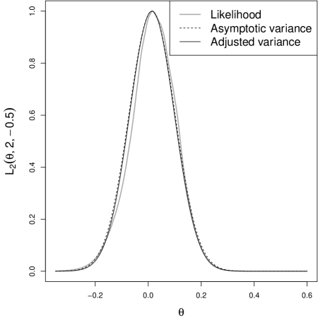 |
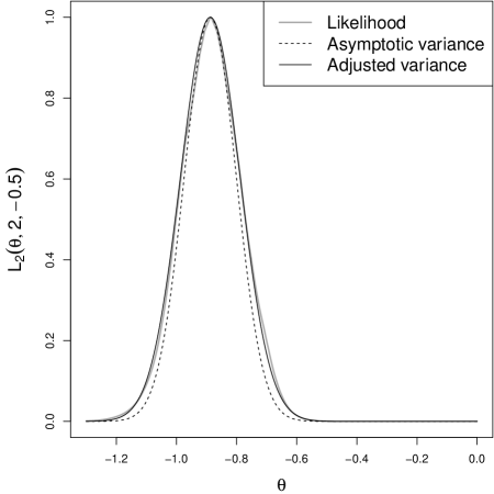 |
11. Supplementary results
| Simulation truth | ||||
| Fitted model | ||||
| Normal | 76.99 | 98.84 | 103.84 | 101.25 |
| ANormal | 92.08 | 86.10 | 102.60 | 115.64 |
| Laplace | 90.58 | 92.84 | 97.90 | 93.13 |
| ALaplace | 122.64 | 121.12 | 124.69 | 131.50 |
| Simulation truth | ||||
| Fitted model | ||||
| Normal | 76.62 | 96.05 | 99.85 | 97.78 |
| ANormal | 81.77 | 82.74 | 92.67 | 104.76 |
| Laplace | 90.29 | 93.42 | 92.88 | 91.25 |
| ALaplace | 117.30 | 113.69 | 115.08 | 122.79 |
| Simulation truth | ||||
|---|---|---|---|---|
| Normal | 6.9 | 29.7 | 6.4 | 32.9 |
| ANormal | 52.9 | 21.9 | 41.3 | 22.2 |
| Laplace | 17.0 | 28.2 | 14.6 | 26.6 |
| ALaplace | 57.7 | 26.4 | 26.7 | 22.4 |
| Inferred | 6.1 | 22.6 | 13.5 | 23.0 |
11.1. Simulation study with identically distributed errors
| Truth | Average | |||
|---|---|---|---|---|
| , , Laplace | ||||
| 0.91 | 0.02 | 0.06 | 0.00 | |
| 0.11 | 0.81 | 0.01 | 0.06 | |
| 0.14 | 0.00 | 0.84 | 0.02 | |
| 0.02 | 0.12 | 0.01 | 0.85 | |
| , , Monte Carlo | ||||
| 0.91 | 0.02 | 0.06 | 0.00 | |
| 0.11 | 0.81 | 0.01 | 0.07 | |
| 0.12 | 0.01 | 0.85 | 0.02 | |
| 0.02 | 0.12 | 0.01 | 0.85 | |
| , , Laplace | ||||
| 0.87 | 0.07 | 0.06 | 0.01 | |
| 0.07 | 0.86 | 0.01 | 0.07 | |
| 0.13 | 0.01 | 0.79 | 0.07 | |
| 0.01 | 0.13 | 0.01 | 0.85 | |
| Truth | Average | |||
|---|---|---|---|---|
| , | ||||
| 0.91 | 0.01 | 0.08 | 0.00 | |
| 0.03 | 0.86 | 0.00 | 0.11 | |
| 0.15 | 0.01 | 0.83 | 0.02 | |
| 0.00 | 0.13 | 0.01 | 0.86 | |
| , | ||||
| 0.89 | 0.01 | 0.10 | 0.00 | |
| 0.02 | 0.89 | 0.00 | 0.09 | |
| 0.15 | 0.01 | 0.82 | 0.02 | |
| 0.00 | 0.16 | 0.01 | 0.83 | |
| , | ||||
| 0.85 | 0.00 | 0.14 | 0.00 | |
| 0.01 | 0.85 | 0.01 | 0.14 | |
| 0.18 | 0.00 | 0.80 | 0.02 | |
| 0.00 | 0.15 | 0.00 | 0.84 | |
| , | ||||
| 0.83 | 0.00 | 0.16 | 0.00 | |
| 0.00 | 0.87 | 0.00 | 0.12 | |
| 0.19 | 0.00 | 0.79 | 0.01 | |
| 0.00 | 0.22 | 0.00 | 0.77 | |
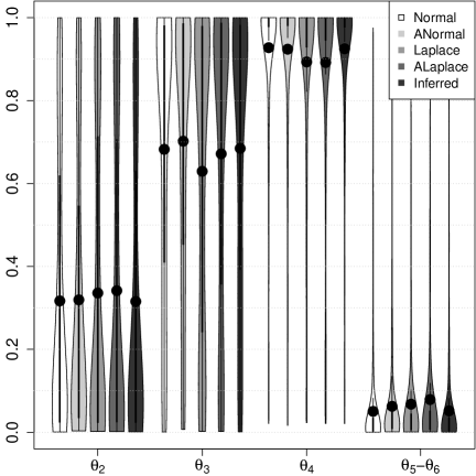 |
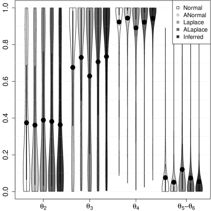 |
 |
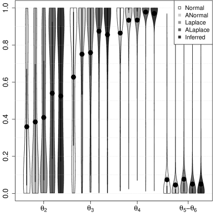 |
 |
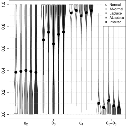 |
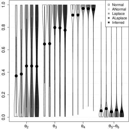 |
 |
| FP | TP | FP | TP | |||||
|---|---|---|---|---|---|---|---|---|
| Truly | ||||||||
| Normal | 0.46 | 0.63 | 0.1 | 2.7 | 0.26 | 0.37 | 0.2 | 2.4 |
| Two-piece Normal | 0.43 | 0.63 | 0.2 | 2.7 | 0.24 | 0.38 | 0.3 | 2.4 |
| Laplace | 0.26 | 0.42 | 0.5 | 2.6 | 0.12 | 0.19 | 0.8 | 2.3 |
| Two-piece Laplace | 0.23 | 0.39 | 0.7 | 2.6 | 0.12 | 0.21 | 0.9 | 2.3 |
| Inferred | 0.45 | 0.62 | 0.2 | 2.7 | 0.25 | 0.37 | 0.2 | 2.4 |
| LASSO-LS | 0.00 | 12.4 | 3.0 | 0.00 | 20.4 | 2.9 | ||
| LASSO-LAD | 0.00 | 10.2 | 2.9 | 0.00 | 18.7 | 2.6 | ||
| LASSO-QR | 0.00 | 10.2 | 2.9 | 0.00 | 18.7 | 2.6 | ||
| SCAD | 0.07 | 4.2 | 2.9 | 0.01 | 7.3 | 2.8 | ||
| Truly | ||||||||
| Normal | 0.38 | 0.55 | 0.2 | 2.6 | 0.21 | 0.34 | 0.5 | 2.4 |
| Two-piece Normal | 0.59 | 0.73 | 0.1 | 2.8 | 0.40 | 0.55 | 0.4 | 2.6 |
| Laplace | 0.20 | 0.35 | 0.7 | 2.5 | 0.07 | 0.14 | 1.2 | 2.4 |
| Two-piece Laplace | 0.33 | 0.48 | 0.5 | 2.7 | 0.18 | 0.32 | 1.1 | 2.5 |
| Inferred | 0.57 | 0.72 | 0.1 | 2.8 | 0.38 | 0.52 | 0.4 | 2.6 |
| LASSO-LS | 0.00 | 12.4 | 3.0 | 0.00 | 21.9 | 2.9 | ||
| LASSO-LAD | 0.00 | 9.8 | 2.8 | 0.00 | 18.1 | 2.6 | ||
| LASSO-QR | 0.00 | 9.0 | 2.9 | 0.00 | 15.1 | 2.7 | ||
| SCAD | 0.07 | 4.0 | 2.9 | 0.03 | 7.3 | 2.8 | ||
| Truly | ||||||||
| Normal | 0.11 | 0.14 | 0.3 | 2.0 | 0.03 | 0.02 | 0.6 | 1.6 |
| Two-piece Normal | 0.11 | 0.15 | 0.3 | 2.1 | 0.04 | 0.04 | 1.1 | 1.7 |
| Laplace | 0.29 | 0.38 | 0.2 | 2.4 | 0.13 | 0.19 | 0.4 | 2.0 |
| Two-piece Laplace | 0.28 | 0.35 | 0.3 | 2.4 | 0.12 | 0.18 | 0.5 | 2.0 |
| Inferred | 0.28 | 0.38 | 0.2 | 2.4 | 0.12 | 0.18 | 0.4 | 2.0 |
| LASSO-LS | 0.00 | 11.3 | 2.8 | 0.00 | 21.4 | 2.5 | ||
| LASSO-LAD | 0.01 | 9.7 | 2.8 | 0.00 | 17.8 | 2.5 | ||
| LASSO-QR | 0.01 | 9.7 | 2.8 | 0.00 | 17.8 | 2.5 | ||
| SCAD | 0.02 | 5.0 | 2.7 | 0.00 | 9.0 | 2.4 | ||
| Truly | ||||||||
| Normal | 0.07 | 0.10 | 0.4 | 1.9 | 0.02 | 0.02 | 1.1 | 1.5 |
| Two-piece Normal | 0.21 | 0.27 | 0.2 | 2.2 | 0.11 | 0.15 | 0.3 | 2.0 |
| Laplace | 0.16 | 0.19 | 0.4 | 2.1 | 0.05 | 0.07 | 0.7 | 1.8 |
| Two-piece Laplace | 0.43 | 0.51 | 0.2 | 2.5 | 0.27 | 0.34 | 0.4 | 2.3 |
| Inferred | 0.41 | 0.48 | 0.2 | 2.5 | 0.25 | 0.33 | 0.4 | 2.2 |
| LASSO-LS | 0.00 | 11.6 | 2.8 | 0.00 | 20.1 | 2.5 | ||
| LASSO-LAD | 0.00 | 9.9 | 2.7 | 0.00 | 17.5 | 2.3 | ||
| LASSO-QR | 0.00 | 9.0 | 2.8 | 0.00 | 15.2 | 2.5 | ||
| SCAD | 0.01 | 5.2 | 2.6 | 0.01 | 9.4 | 2.3 | ||
| FP | TP | FP | TP | |||||
|---|---|---|---|---|---|---|---|---|
| Truly | ||||||||
| Normal | 0.01 | 0.01 | 0.4 | 1.2 | 0.00 | 0.00 | 0.8 | 0.9 |
| Two-piece Normal | 0.01 | 0.01 | 0.5 | 1.2 | 0.00 | 0.00 | 0.9 | 0.8 |
| Laplace | 0.00 | 0.00 | 0.7 | 1.1 | 0.00 | 0.00 | 1.0 | 0.8 |
| Two-piece Laplace | 0.00 | 0.01 | 0.8 | 1.1 | 0.00 | 0.00 | 1.1 | 0.8 |
| Inferred | 0.01 | 0.01 | 0.5 | 1.2 | 0.00 | 0.00 | 0.7 | 0.9 |
| LASSO-LS | 0.00 | 11.9 | 2.5 | 0.00 | 18.0 | 2.0 | ||
| LASSO-LAD | 0.00 | 8.9 | 2.0 | 0.00 | 15.6 | 1.4 | ||
| LASSO-QR | 0.00 | 8.9 | 2.0 | 0.00 | 15.6 | 1.4 | ||
| SCAD | 0.00 | 6.3 | 2.3 | 0.01 | 10.4 | 1.8 | ||
| Truly | ||||||||
| Normal | 0.00 | 0.00 | 0.5 | 1.2 | 0.00 | 0.00 | 0.7 | 0.9 |
| Two-piece Normal | 0.01 | 0.01 | 0.4 | 1.4 | 0.00 | 0.01 | 0.7 | 1.1 |
| Laplace | 0.00 | 0.00 | 0.9 | 1.0 | 0.00 | 0.00 | 1.4 | 0.7 |
| Two-piece Laplace | 0.01 | 0.01 | 0.7 | 1.2 | 0.00 | 0.00 | 1.5 | 1.0 |
| Inferred | 0.01 | 0.01 | 0.4 | 1.4 | 0.00 | 0.01 | 0.9 | 1.0 |
| LASSO-LS | 0.00 | 11.0 | 2.4 | 0.00 | 19.4 | 1.9 | ||
| LASSO-LAD | 0.00 | 8.6 | 1.8 | 0.00 | 15.3 | 1.4 | ||
| LASSO-QR | 0.00 | 8.1 | 2.1 | 0.00 | 12.8 | 1.5 | ||
| SCAD | 0.00 | 6.1 | 2.1 | 0.00 | 10.1 | 1.8 | ||
| Truly | ||||||||
| Normal | 0.01 | 0.01 | 0.4 | 1.3 | 0.00 | 0.00 | 0.8 | 0.9 |
| Two-piece Normal | 0.01 | 0.01 | 0.5 | 1.3 | 0.00 | 0.00 | 0.9 | 1.0 |
| Laplace | 0.05 | 0.06 | 0.4 | 1.7 | 0.01 | 0.01 | 0.7 | 1.2 |
| Two-piece Laplace | 0.05 | 0.07 | 0.4 | 1.7 | 0.01 | 0.01 | 0.8 | 1.2 |
| Inferred | 0.04 | 0.04 | 0.3 | 1.7 | 0.01 | 0.01 | 0.7 | 1.2 |
| LASSO-LS | 0.00 | 10.8 | 2.5 | 0.00 | 20.4 | 2.0 | ||
| LASSO-LAD | 0.01 | 9.3 | 2.5 | 0.00 | 17.1 | 2.0 | ||
| LASSO-QR | 0.01 | 9.3 | 2.5 | 0.00 | 17.1 | 2.0 | ||
| SCAD | 0.00 | 5.9 | 2.2 | 0.00 | 10.3 | 1.8 | ||
| Truly | ||||||||
| Normal | 0.00 | 0.00 | 0.5 | 1.1 | 0.00 | 0.00 | 0.9 | 0.8 |
| Two-piece Normal | 0.02 | 0.01 | 0.4 | 1.5 | 0.01 | 0.01 | 0.6 | 1.2 |
| Laplace | 0.02 | 0.01 | 0.6 | 1.3 | 0.00 | 0.01 | 0.8 | 1.0 |
| Two-piece Laplace | 0.09 | 0.12 | 0.3 | 1.9 | 0.04 | 0.05 | 0.7 | 1.5 |
| Inferred | 0.09 | 0.10 | 0.3 | 1.8 | 0.04 | 0.05 | 0.6 | 1.4 |
| LASSO-LS | 0.00 | 10.9 | 2.3 | 0.00 | 18.0 | 1.8 | ||
| LASSO-LAD | 0.00 | 9.4 | 2.3 | 0.00 | 15.6 | 1.7 | ||
| LASSO-QR | 0.00 | 8.3 | 2.5 | 0.00 | 14.0 | 2.0 | ||
| SCAD | 0.01 | 5.7 | 2.1 | 0.00 | 10.2 | 1.6 | ||
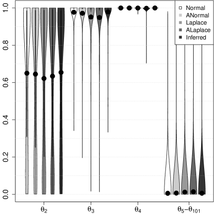 |
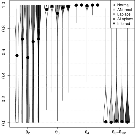 |
 |
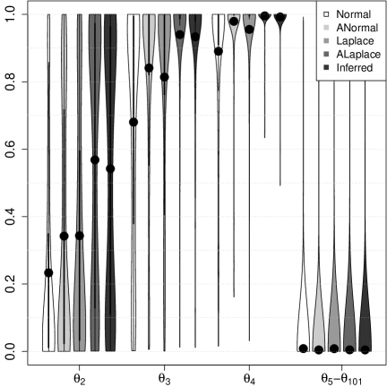 |
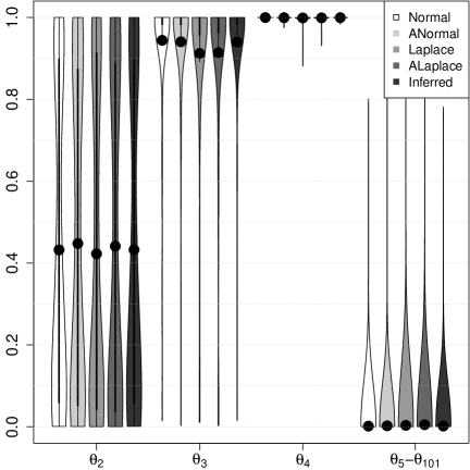 |
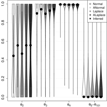 |
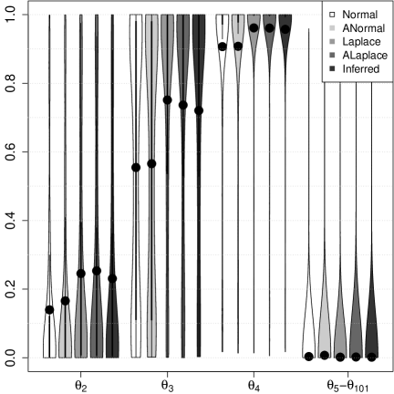 |
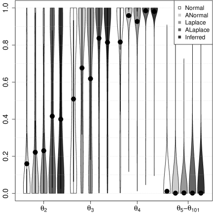 |
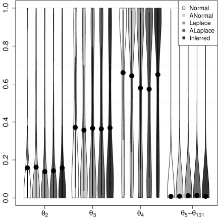 |
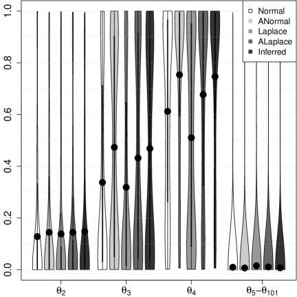 |
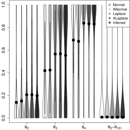 |
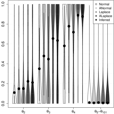 |
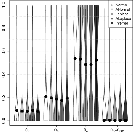 |
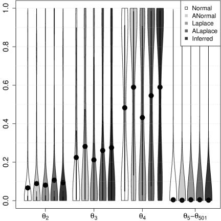 |
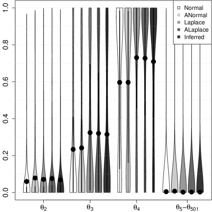 |
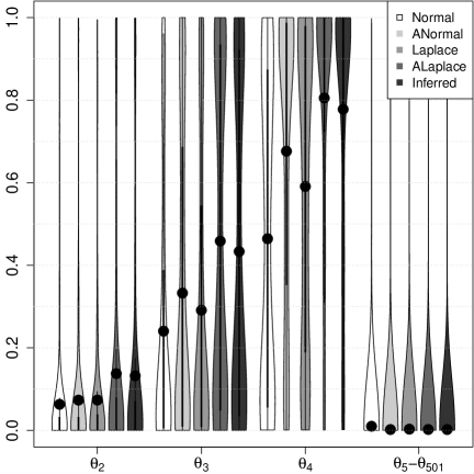 |
We assessed the sensitivity of the results of the simulation study in Section 6.1 of the main paper to the prior on the asymmetry coefficient by setting such that . Supplementary Table 4 summarizes the inference on the error distribution and Supplementary Figure 7 the marginal variable inclusion probabilities. The latter were virtually identical to those in Figure 2 obtained under such that , showing that variable inclusion is robust to moderate changes in .
We also assessed the accuracy of the Laplace approximations to the integrated likelihood by comparing the results with those obtained with the importance sampling estimates with draws described in Section 5 of the main paper. Supplementary Figure 8 displays the results for . These are extremely similar to those based on Laplace approximation in Figure 2.
Supplementary Figure 11 shows analogous results for , with and estimated via Laplace approximations.
11.2. Simulation study with non-identically distributed errors
| Truth | Average | |||
|---|---|---|---|---|
| 0.000 | 0.000 | 0.914 | 0.086 | |
| 0.000 | 0.003 | 0.096 | 0.901 | |
| 0.000 | 0.000 | 0.906 | 0.094 | |
| 0.000 | 0.000 | 0.053 | 0.947 | |
| 0.425 | 0.834 | 0.961 | 0.017 | 0.015 | |
| 0.751 | 0.950 | 0.996 | 0.016 | 0.015 | |
| 0.796 | 0.970 | 0.999 | 0.020 | 0.016 | |
| 0.769 | 0.969 | 0.999 | 0.016 | 0.012 | |
| 0.473 | 0.912 | 0.987 | 0.016 | 0.016 |
| Normal | ANormal |
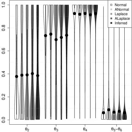 |
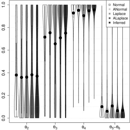 |
| Laplace | ALaplace |
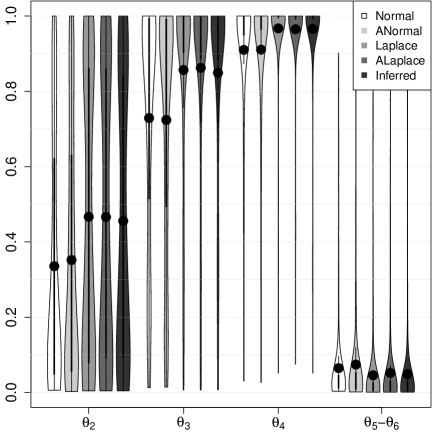 |
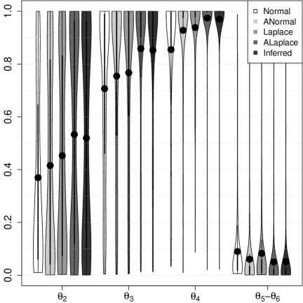 |
| TP | FP | |
| Zellner, Normal errors | 2.8 | 21.3 |
| pMOM, Normal errors | 3.0 | 12.0 |
| pMOM, inferred errors | 2.8 | 10.5 |
| peMOM, Normal errors | 1.9 | 2.9 |
Supplementary Table 8 shows the mean average posterior probability assigned to the Normal, asymmetric Normal, Laplace and asymmetric Laplace models under the heteroskedastic simulation (Section 6.2, main manuscript).
Supplementary Figure 13 shows marginal variable inclusion probabilities under the hetero-asymmetric simulation.
11.3. DLD data
| Gene symbol | Normal | Inferred |
| C6orf226 | 1.000 | 1.000 |
| ECH1 | 1.000 | 1.000 |
| CSF2RA | 1.000 | 1.000 |
| RRP1B | 0.944 | 0.999 |
| FBXL19 | 0.993 | 0.658 |
| MTMR1 | 0.183 | 0.467 |
| SLC35B4 | 0.209 | 0.332 |
| RAB3GAP2 | 0.007 | 0.040 |
| Model | |
| C6orf226, ECH1, CSF2RA, FBXL19, RRP1B | 0.384 |
| SLC35B4, C6orf226, ECH1, CSF2RA, RRP1B | 0.349 |
| SLC35B4, C6orf226, MTMR1, ECH1, CSF2RA, RRP1B | 0.127 |
| C6orf226, MTMR1, ECH1, CSF2RA, FBXL19, RRP1B | 0.049 |
| C6orf226, MTMR1, RAB3GAP2, ECH1, CSF2RA, RRP1B | 0.023 |
| Model | |
| C6orf226, MTMR1, ECH1, CSF2RA, FBXL19, RRP1B | 0.454 |
| C6orf226, ECH1, CSF2RA, FBXL19, RRP1B | 0.258 |
| SLC35B4, C6orf226, MTMR1, ECH1, CSF2RA, RRP1B | 0.108 |
| SLC35B4, C6orf226, ECH1, CSF2RA, RRP1B | 0.061 |
| C6orf226, MTMR1, RAB3GAP2, ECH1, CSF2RA, RRP1B | 0.016 |
| Model | |
| C6orf226, ECH1, CSF2RA, FBXL19, RRP1B | 0.399 |
| SLC35B4, C6orf226, ECH1, CSF2RA, RRP1B | 0.359 |
| SLC35B4, C6orf226, MTMR1, ECH1, CSF2RA, RRP1B | 0.120 |
| C6orf226, MTMR1, ECH1, CSF2RA, FBXL19, RRP1B | 0.051 |
| SLC35B4, C6orf226, RAB3GAP2, ECH1, CSF2RA, RRP1B | 0.008 |
Supplementary Table 11 shows the six genes with largest marginal inclusion probabilities when conditioning on Normal errors and when inferring the error distribution. The figures were similar for the four top genes, but the Normal model assigned somewhat higher probability to FBXL19 substantially lower probability to MTMR1.
References
- Alfons et al. [2013] A. Alfons, C. Croux, and S. Gelper. Sparse least trimmed squares regression for analyzing high-dimensional large data sets. The Annals of Applied Statistics, 7(1):226–248, 2013.
- Arellano-Valle et al. [2005] R.B. Arellano-Valle, H.W. Gómez, and F.A. Quintana. Statistical inference for a general class of asymmetric distributions. Journal of Statistical Planning and Inference, 128(2):427–443, 2005.
- Arslan [2012] O. Arslan. Weighted LAD-LASSO method for robust parameter estimation and variable selection in regression. Computational Statistics and Data Analysis, 56(6):1952–1965, 2012.
- Barbieri and Berger [2004] M.M. Barbieri and J.O. Berger. Optimal predictive model selection. The Annals of Statistics, 32(3):870–897, 2004.
- Bayarri et al. [2012] M.J. Bayarri, J.O. Berger, A. Forte, and G. Garcia-Donato. Criteria for Bayesian model choice with application to variable selection. The Annals of statistics, 40(3):1550–1577, 2012.
- Breheny and Huang [2011] P. Breheny and J. Huang. Coordinate descent algorithms for nonconvex penalized regression, with applications to biological feature selection. Annals of Applied Statistics, 5(1):232–253, 2011.
- Calon et al. [2012] A. Calon, E. Espinet, S. Palomo-Ponce, D.V.F. Tauriello, M. Iglesias, M.V. Céspedes, M. Sevillano, C. Nadal, P. Jung, X.H.-F. Zhang, D. Byrom, A. Riera, D. Rossell, R. Mangues, J. Massague, E. Sancho, and E. Batlle. Dependency of colorectal cancer on a tgf-beta-driven programme in stromal cells for metastasis initiation. Cancer Cell, 22(5):571–584, 2012.
- Chae et al. [2016] M. Chae, L. Lin, and D.B. Dunson. Bayesian sparse linear regression with unknown symmetric error. arXiv, 1608.02143:1–34, 2016.
- Chung and Dunson [2009] Y. Chung and D.B. Dunson. Nonparametric bayes conditional distribution modeling with variable selection. Journal of the American Statistical Association, 104(488):1646–1660, 2009.
- Daye et al. [2012] Z.J. Daye, J. Chen, and H. Li. High-dimensional heteroscedastic regression with an application to eqtl data analysis. Biometrics, 68(1):316–326, 2012.
- Dette et al. [2016] H. Dette, C. Ley, and F.J. Rubio. Natural (non-) informative priors for skew-symmetric distributions. arXiv preprint arXiv:1605.02880, 2016.
- Eicker [1964] F. Eicker. Asymptotic normality and consistency of the least squares estimator for families of linear regressions. Annals of Mathematical Statistics, 34(2):447–456, 1964.
- Fan and Li [2001] J. Fan and R. Li. Variable selection via nonconcave penalized likelihood and its oracle properties. Journal of the American Statistical Association, 96(456):1348–1360, 2001.
- Fan et al. [2014] J. Fan, Y. Fan, and E. Barut. Adaptive robust variable selection. The Annals of Applied Statistics, 42(1):324–351, 2014.
- Fernández and Steel [1998] C. Fernández and M.F.J. Steel. On Bayesian modeling of fat tails and skewness. Journal of the American Statistical Association, 93(441):359–371, 1998.
- Gijbels and Vrinssen [2015] I. Gijbels and I. Vrinssen. Robust nonnegative garrote variable selection in linear regression. Computational Statistics and Data Analysis, 85:1–22, 2015.
- Gottardo and Raftery [2007] R. Gottardo and A.E. Raftery. Bayesian robust transformation and variable selection: a unified approach. The Canadian Journal of Statistics, 37(3):361–380, 2007.
- Grünwald and van Ommen [2014] P. Grünwald and T. van Ommen. Inconsistency of Bayesian inference for misspecified linear models, and a proposal for repairing it. arXiv, 1412.3730:1–70, 2014.
- Huber [1973] P.J. Huber. Robust regression: asymptotics, conjectures and Monte Carlo. The Annals of Statistics, 1(5):799–821, 1973.
- Johnson [2013] V.E. Johnson. On numerical aspects of Bayesian model selection in high and ultrahigh-dimensional settings. Bayesian Analysis, 8(4):741, 2013.
- Johnson and Rossell [2010] V.E. Johnson and D. Rossell. Prior densities for default Bayesian hypothesis tests. Journal of the Royal Statistical Society B, 72(2):143–170, 2010.
- Johnson and Rossell [2012] V.E. Johnson and D. Rossell. Bayesian model selection in high-dimensional settings. Journal of the American Statistical Association, 24(498):649–660, 2012.
- Kimber [1985] A. C. Kimber. Methods for the two-piece normal distribution. Communications in Statistics - Theory and Methods, 14(1):235–245, 1985.
- Knight [1999] K. Knight. Asymptotics for l1-estimators of regression parameters under heteroscedasticity. The Canadian Journal of Statistics, 27(3):497–507, 1999.
- Kocherginsky et al. [2005] M. Kocherginsky, X. He, and Y. Mu. Practical confidence intervals for regression quantiles. Journal of Computational and Graphical Statistics, 14(1):41–55, 2005.
- Koenker [1994] R. Koenker. Confidence intervals for regression quantiles. In Proceedings of the 5th Prague Symposium on Asymptotic Statistics, pages 349–359. Springer-Verlag, 1994.
- Koenker [2005] R. Koenker. Quantile regression. Cambridge University Press, Cambridge, 2005.
- Koenker and Bassett [1982] R. Koenker and G. Bassett. Tests of linear hypotheses and l1 estimation. Econometrica, 50(6):1577–1584, 1982.
- Kundu and Dunson [2014] S. Kundu and D.B. Dunson. Bayes variable selection in semiparametric linear models. Journal of the American Statistical Association, 109(505):437–447, 2014.
- Lambert-Lacroix [2011] S. Lambert-Lacroix. Robust regression through the huber’s criterion and adaptive lasso penalty. Electronic Journal of Statistics, 5:1015–1053, 2011.
- Levenberg [1944] K. Levenberg. A method for the solution of certain non-linear problems in least squares. Quarterly of Applied Mathematics, 2(2):164–168, 1944.
- Loh [2017] P.-L. Loh. Statistical consistency and asymptotic normality for high-dimensional robust M-estimators. The Annals of Statistics, 45(2):866–896, 2017.
- Mallick and Nengjun [2013] H. Mallick and Y. Nengjun. Bayesian methods for high dimensional linear models. Journal of Biometrics & Biostatistics, 1:005, 2013.
- Marquardt [1963] D. Marquardt. An algorithm for least-squares estimation of nonlinear parameters. SIAM Journal on Applied Mathematics, 11(2):431–441, 1963.
- Mendelson [2014] S. Mendelson. Learning without concentration for general loss functions. ArXiv, 1410.3192, 2014.
- Mudholkar and Hutson [2000] G.S Mudholkar and A.D. Hutson. The epsilon-skew-normal distribution for analyzing near-normal data. Journal of Statistical Planning and Inference, 83(2):291–309, 2000.
- Newey and Powell [1987] W. K. Newey and J. L. Powell. Asymmetric least squares estimation and testing. Econometrica, 55(4):819–847, 1987.
- Pollard [1991] D. Pollard. Asymptotics for least absolute deviation regression estimators. Econometric Theory, 7(2):186–199, 1991.
- Rockafellar [2015] R.T. Rockafellar. Convex analysis. Princeton university press, Princeton, 2015.
- Rossell and Telesca [2017] D. Rossell and D. Telesca. Non-local priors for high-dimensional estimation. Journal of the American Statistical Association, 112:254–265, 2017.
- Rossell et al. [2013] D. Rossell, D. Telesca, and V.E. Johnson. High-dimensional Bayesian classifiers using non-local priors. In Statistical Models for Data Analysis XV, pages 305–314. Springer, 2013.
- Rossell et al. [2016] D. Rossell, J.D. Cook, D. Telesca, and P. Roebuck. mombf: Moment and Inverse Moment Bayes Factors, 2016. URL https://CRAN.R-project.org/package=mombf. R package version 1.8.1.
- Rubio and Genton [2016] F.J. Rubio and M.G. Genton. Bayesian linear regression with skew-symmetric error distributions with applications to survival analysis. Statistics in Medicine, 35(4):2441–2454, 2016.
- Rubio and Steel [2014] F.J. Rubio and M.F.J. Steel. Inference in two-piece location-scale models with jeffreys priors (with discussion). Bayesian Analysis, 9(1):1–22, 2014.
- Rubio and Yu [2017] F.J. Rubio and K. Yu. Flexible objective Bayesian linear regression with applications in survival analysis. Journal of Applied Statistics, 44, 2017.
- Scott and Berger [2010] J.G. Scott and J.O Berger. Bayes and empirical Bayes multiplicity adjustment in the variable selection problem. The Annals of Statistics, 38(5):2587–2619, 2010.
- Shin et al. [2015] M. Shin, A. Bhattacharya, and V.E. Johnson. Scalable Bayesian variable selection using nonlocal prior densities in ultrahigh-dimensional settings. Texas A&M University (technical report), pages 1–33, 2015.
- Sorensen [1982] D.C. Sorensen. Newton’s method with a model trust region modification. SIAM Journal of Numerical Analysys, 19(2):409–426, 1982.
- Srivastava [1971] M.S. Srivastava. On fixed width confidence bounds for regression parameters. The Annals of Mathematical Statistics, 42(4):1403–1411, 1971.
- Tibshirani [1996] R. Tibshirani. Regression shrinkage and selection via the Lasso. Journal of the Royal Statistical Society, B, 58(1):267–288, 1996.
- van der Vaart [1998] A.W. van der Vaart. Asymptotic statistics. Cambridge University Press, New York, 1998.
- Wallis [2014] K.F. Wallis. The two-piece normal, binormal, or double Gaussian distribution: its origin and rediscoveries. Statistical Science, 29(1):106–112, 2014.
- Wang et al. [2007] H. Wang, G. Li, and G. Jiang. Robust regression shrinkage and consistent variable selection through the LAD-LASSO. Journal of Business & Economic Statistics, 25(3):347–355, 2007.
- Wang and Li [2009] L. Wang and R. Li. Weighted Wilcoxon-type smoothly clipped absolute deviation method. Biometrics, 65(2):564–571, 2009.
- Wang et al. [2016] L. Wang, Y. Tang, D. Sinha, D. Pati, and S. Lipsitz. Bayesian variable selection for skewed heteroscedastic response. arXiv preprint arXiv:1602.09100, 2016.
- Wu and Liu [2009] L. Wu and Y. Liu. Variable selection in quantile regression. Statistica Sinica, 19(2):801–809, 2009.
- Yan and Kottas [2015] Y. Yan and A. Kottas. A new family of error distributions for Bayesian quantile regression. Technical report, University of California Santa Cruz, 2015.
- Yu et al. [2013] K. Yu, C.W.S. Chen, C. Reed, and D.B. Dunson. Bayesian variable selection in quantile regression. Statistics and its Interface, 6(2):261–274, 2013.
- Yuan et al. [2016] T. Yuan, X. Huang, M. Woodcock, M. Du, R. Dittmar, Y. Wang, S. Tsai, M. Kohli, L. Boardman, T. Patel, and L. Wang. Plasma extracellular rna profiles in healthy and cancer patients. Scientific Reports, 6:1–11, 2016.