Quintessential Scale Dependence from Separate Universe Simulations

Abstract

By absorbing fluctuations into a local background, separate universe simulations provide a powerful technique to characterize the response of small-scale observables to the long-wavelength density fluctuations, for example those of the power spectrum and halo mass function which lead to the squeezed-limit $n$-point function and halo bias, respectively. Using quintessence dark energy as the paradigmatic example, we extend these simulation techniques to cases where non-gravitational forces in other sectors establish a Jeans scale across which the growth of density fluctuations becomes scale dependent. By characterizing the separate universes with matching background expansion histories, we show that the power spectrum and mass function responses depend on whether the long-wavelength mode is above or below the Jeans scale. Correspondingly, the squeezed bispectrum and halo bias also become scale dependent. Models of bias that are effectively local in the density field at a single epoch, initial or observed, cannot describe this effect which highlights the importance of temporal nonlocality in structure formation. Validated by these quintessence tests, our techniques are applicable to a wide range of models where the complex dynamics of additional fields affect the clustering of matter in the linear regime and it would otherwise be difficult to simulate their impact in the nonlinear regime.

I Introduction

The coupling between density fluctuations of different wavelengths is one of the most important topics in the study of large-scale structure Bernardeau et al. (2002). These couplings can be imprinted in the inflationary initial conditions or develop through gravitational evolution. In the latter class, a long-wavelength density mode affects the evolution of all short-wavelength modes that are embedded in it leading to changes in the power spectrum Takada and Hu (2013); Li et al. (2014a); Chiang et al. (2014, 2015) and the dark matter halo abundance which gives rise to halo bias Mo and White (1996); Seljak (2012). In the limit of a large separation in these scales, one can use the “separate universe” (SU) approach to describe these and other effects through a change in the background density within which small scale structure evolves Barrow and Saich (1993); Baldauf et al. (2011); Sherwin and Zaldarriaga (2012).

The SU approach is not only conceptually straightforward to understand but can also be readily implemented in cosmological simulations, arbitrarily deep into the nonlinear regime where perturbation theory breaks down Sirko (2005); Gnedin et al. (2011); Li et al. (2014b); Wagner et al. (2015a). In particular, SU simulations have enabled studies of the squeezed-limit $n$-point correlation functions Wagner et al. (2015b) and their impact on the power spectrum covariance Li et al. (2014b), the halo bias Li et al. (2016); Lazeyras et al. (2016); Baldauf et al. (2015), and the Lyman-$\alpha$ forest McDonald (2003); Cieplak and Slosar (2016). Since the whole time evolution of the long-wavelength mode is properly captured, as opposed to just a single epoch such as the time of observation, temporally nonlocal effects on small-scale observables such as the nonlinear power spectrum Ma (2007) and halo bias Senatore (2015); LoVerde (2014a) are correctly modeled.

Previous studies have focused on SU simulations in the $\Lambda$CDM cosmology, where only matter clusters at low redshift. If the system contains additional clustering components such as dynamic dark energy or massive neutrinos, then one has to be careful when applying the separate universe principle. Specifically, the separate universe construction is only strictly true if long-wavelength perturbations evolve under gravitational forces alone and not internal stress gradients Dai et al. (2015); Hu et al. (2016). This means that a SU description would seem to require that the long-wavelength mode be larger than the Jeans or free streaming scale of the system. On the other hand, if the impact on small-scale structure of these extra components is only gravitational, then it can be correctly modeled by matching the local expansion rate to an SU Hubble rate in a “fake” SU approach which implicitly requires fictitious energy density components Hu et al. (2016).

In this work, we implement and test this multi-component SU method in simulations with quintessence dark energy. In particular, the growth of long-wavelength matter fluctuations above or below the Jeans scale of quintessence differs due to clustering of the dark energy. As a result, the SU expansion history depends on the scale of the long-wavelength matter fluctuation as does the response of small-scale observables such as the power spectrum and halo mass function. The latter implies that halo bias itself will become scale dependent.

The rest of the paper is organized as follows. In Sec. II, we describe the mapping of perturbations in the quintessence model onto the SU background above and below the Jeans scale. In Sec. III, we implement the SU approach in quintessence simulations. We present the results of SU simulations in Sec. IV and Sec. V for the power spectrum response and the halo bias respectively. We discuss these results in Sec. VI. In Appendix A, we compare our results to the predictions of scale-dependent halo bias models in the recent literature.

Throughout the paper, we adopt a spatially flat cosmology with a Hubble constant $h=0.7$, matter density $\Omega_{m}=0.3$, quintessence energy density $\Omega_{Q}=0.7$, quintessence equation of state $w_{Q}=-0.5$, and an initial curvature power spectrum with scale-invariant tilt $n_{s}=1$ and amplitude which sets $\sigma_{8}=1$ today. These parameters are chosen to highlight the scale dependence of quintessence rather than for observational viability.

II Quintessential Separate Universe

Following Ref. Hu et al. (2016), we review here the construction of the separate universe for the case where components other than the cold dark matter possess Jeans scales. In Sec. II.1, we show that the influence of these components is captured by a modified expansion history that is defined by the growth history of the large-scale matter density fluctuation. We apply this construction to quintessence dark energy models in Sec. II.2.

II.1 Expansion History

A observer sitting within a long-wavelength matter fluctuation $\delta_{m}$ would measure the local mean matter density as

$$\bar{\rho}_{mW}(a)=\bar{\rho}_{m}(a)[1+\delta_{m}(a)]\,,$$ (1)

where $W$ denotes a windowed average across a scale much smaller than the long-wavelength mode. In the SU picture, the local mean evolves as if the observer were in a SU whose scale factor

$$a_{W}=\frac{a}{(1+\delta_{m})^{1/3}}\approx a\left(1-\frac{\delta_{m}}{3}\right)\,,$$ (2)

so that $\bar{\rho}_{mW}\propto a_{W}^{-3}$. Note that at early times

$$\lim_{t\to 0}\delta_{m}\to 0\,,~{}~{}\lim_{t\to 0}a_{W}\to a\,,$$ (3)

and the physical conditions of the local and global cosmology coincide. We have implicitly assumed that there is a universal time coordinate between the two and so in the relativistic limit $\delta_{m}$ is specifically the synchronous gauge density perturbation Hu et al. (2016).

Notice that the SU construction requires only $\delta_{m}(a)$ itself, not the evolution of any other density component in the universe. The other components determine the evolution of $\delta_{m}(a)$, but they do not enter into $a_{W}$ explicitly. If these components only influence small-scale observables through their impact on $\delta_{m}(a)$, their effects can be characterized by $a_{W}$ and the local Hubble expansion

$$H_{W}=\frac{\dot{a}_{W}}{a_{W}}=H-\frac{1}{3}\dot{\delta}_{m}=H\left(1-\frac{1}{3}\delta^{\prime}_{m}\right)\,,$$ (4)

where ${}^{\prime}\equiv d/d\ln a$. This expansion history does not even need to be given by a SU Friedmann equation involving the local energy densities and curvature Gnedin et al. (2011); Hu et al. (2016). With $a_{W}$ and $H_{W}$ alone, we can model the small-scale observables using $N$-body simulations with this SU expansion rate.

This construction includes cases where the other components experience non-gravitational forces which define their Jeans scales. In these cases, the growth history of $\delta_{m}(a)$ depends on scale. Since the SU expansion history depends on the whole growth history, regions of different sizes that share a common $\delta_{m}$ at a fixed $a$ will produce different responses in the small-scale observables. In other words, these observables cannot be described solely by the change in the local density at the time of observation alone. For example, as we shall see in Sec. V, the response of the dark matter halo abundance to $\delta_{m}(a)$ leads to a halo bias that violates the local bias expectation of scale independence in the linear regime.

II.2 Quintessence

Quintessence or scalar field dark energy models provide a simple arena to explore the response of small-scale observables to long-wavelength fluctuations, in particular their amplitude, scale, and growth history. The construction of the SU with quintessence perturbations has been extensively discussed in Ref. Hu et al. (2016). Here we only summarize the results that are related to simulating observable responses above and below the quintessence Jeans scale.

The sound speed of quintessence $c_{Q}$ sets the sound horizon or Jeans scale $r_{J}\sim c_{Q}/aH$ across which its influence on the evolution of $\delta_{m}$ differs. If $\delta_{m}$ has a wavelength smaller than $r_{J}$, the quintessence perturbation is Jeans stable and becomes negligible in comparison. Thus the matter fluctuations evolve under

$$\delta_{\downarrow}^{\prime\prime}+\left(2+\frac{H^{\prime}}{H}\right)\delta_{\downarrow}^{\prime}=\frac{3}{2}\frac{H_{0}^{2}}{H^{2}}\frac{\Omega_{m}}{a^{3}}\delta_{\downarrow}\,,$$ (5)

where $\delta_{m}=\delta_{\downarrow}$ and the down arrow in the subscript denotes the sub-Jeans case. On the other hand, if $\delta_{m}$ has a wavelength larger than $r_{J}$, then the quintessence perturbation $\delta_{Q}$ has an impact on $\delta_{m}$. Assuming that all fluctuations arise from initial curvature fluctuations and the sound speed of quintessence is much smaller than speed of light, we have for the two-component system Hu et al. (2016)

$$\delta^{\prime}_{Q}-3w_{Q}\delta_{Q}\> =(1+w_{Q})\delta_{\uparrow}^{\prime}\,,$$

$$\delta_{\uparrow}^{\prime\prime}+\left(2+\frac{H^{\prime}}{H}\right)\delta_{\uparrow}^{\prime}\> =\frac{3}{2}\frac{H_{0}^{2}}{H^{2}}\left[\frac{\Omega_{m}\delta_{\uparrow}}{a^{3}}+\frac{\Omega_{Q}\delta_{Q}}{a^{3(1+w_{Q})}}\right]\,,$$ (6)

where $\delta_{m}=\delta_{\uparrow}$ and the up arrow in the subscript denotes the super-Jeans case. For simplicity we have also taken the quintessence equation of state parameter $w_{Q}=\bar{p}_{Q}/\bar{\rho}_{Q}$ to be a constant. With the assumed curvature initial conditions, the initial conditions for the fields are set by taking $\delta_{m}=\delta_{\uparrow}=\delta_{\downarrow}$ and $\delta_{Q}$ are all proportional to $a$ in the matter dominated limit.

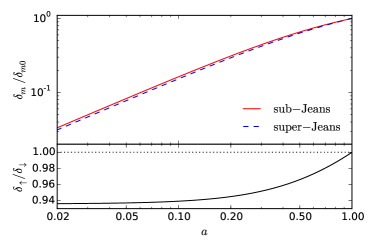
In Fig. 1 we plot $\delta_{m}/\delta_{m0}$ as a function of the global scale factor, where $\delta_{m0}=\delta_{m}(a=1)$ is the present-day overdensity. The red solid and blue dashed lines show the sub-Jeans and super-Jeans SUs. Normalized to the same $\delta_{m0}$, the super-Jeans SU is always closer to the global universe ($\delta_{m}=0$) in the past than the sub-Jeans SU in its expansion history. This implies that the response of the small-scale observables such as the power spectrum and halo abundance should be smaller in the super-Jeans than the sub-Jeans SU.

Figure 1: (Top) Scale-dependent growth in $\delta_{m}$ as a function of the scale factor for super-Jeans (red solid) and sub-Jeans (blue dashed) long-wavelength modes. (Bottom) The ratio of $\delta_{m}$ in super-Jeans to sub-Jeans cases. When characterized as a separate universe, the former is closer to the global universe than the latter in the past for the same density fluctuation today.

Finally for setting up simulations in the next section it is useful to define the linear growth of short-wavelength structure in the SU. If the small-scale matter fluctuations of interest are well within $r_{J}$, the growth function $D_{W}$ is simply Eq. (5) with the SU expansion history

$$\frac{d^{2}D_{W}}{d\ln a_{W}^{2}}+\left(2+\frac{d\ln H_{W}}{d\ln a_{W}}\right)\frac{dD_{W}}{d\ln a_{W}}=\frac{3}{2}\frac{H_{0W}^{2}}{H_{W}^{2}}\frac{\Omega_{mW}}{a_{W}^{3}}D_{W}\,.$$ (7)

Note that

$$\Omega_{mW}H_{0W}^{2}=\Omega_{m}H_{0}^{2}\,,$$ (8)

and so only the SU expansion rate $H_{W}$ from Eq. (4) is required to solve for $D_{W}(a_{W})$. As we shall see next, we can generalize this statement to nonlinear observables with SU $N$-body simulations.

III Separate Universe Simulations

The growth history of the long-wavelength matter fluctuation $\delta_{m}(a)$ in the global universe alone sets the expansion history in the separate universe. All effects from long-wavelength fluctuations in other species are incorporated into its growth history. In the quintessence model, within the Jeans scale dark energy perturbations can be ignored and so the response of small scale observables can be calibrated using $N$-body simulations with just this change in the expansion history.

Unlike the SU technique in $\Lambda$CDM, the change of cosmological parameters and their correspondence with real energy densities and curvature becomes non-trivial for the quintessence model Hu et al. (2016) whereas the direct change in the expansion rate $H_{W}$ remains simply determined by $\delta_{m}(a)$. Thus, while some steps are similar to the $\Lambda$CDM SU techniques for running and analyzing simulations (see e.g. Li et al. (2014b); Wagner et al. (2015a); Li et al. (2016); Lazeyras et al. (2016)), there are some major differences in performing the SU simulations with quintessence which we now describe.

Let us start with setting the initial conditions for the simulations. Recall that at high redshift the separate and global universes are identical in their physical description. To achieve this, we first compute the linear power spectrum with the global cosmology at $z=0$ using CAMB Lewis et al. (2000); Howlett et al. (2012). We then rescale this power spectrum to the initial redshift of the simulations $a_{Wi}=0.02$ as

$$P_{W}(k,a_{Wi})=P(k,a_{0})\left[\frac{D_{W}(a_{Wi})}{D(a_{0})}\right]^{2}\,,$$ (9)

where $D$ is the linear growth in the global universe and $D_{W}$ is the linear growth of the SU following Eq. (7). The growth functions are normalized in the matter dominated epoch as

$$\lim_{a\rightarrow 0}D(a)=a,\quad\lim_{a_{W}\rightarrow 0}D(a_{W})=a_{W}\,.$$ (10)

Note that $D_{W}$ in sub-Jeans and super-Jeans SUs are different, as they have different expansion histories. Another subtlety is that the change in the expansion rate of the SU makes the traditional unit of comoving $[h\,{\rm Mpc}^{-1}]$ inconvenient. Throughout this paper we avoid this confusion by using units of comoving $[{\rm Mpc}]$ and convert for code purposes as necessary. Given the different scale factors $a$ and $a_{W}$, the correspondence between comoving wavenumber and physical wavenumber in the global universe differ. Since this represents a simple dilation of scales, we can account for it in the interpretation of observable responses rather than in the simulations directly Li et al. (2014b).

The initial conditions are then set up using realizations of Gaussian random fields for the primordial fluctuations and evolved to $a_{Wi}$ using second-order Lagrangian perturbation theory (2LPT) Crocce et al. (2006). Usual 2LPT codes, such as the publicly available 2LPTIC Scoccimarro , compute the linear growth and growth rate $f_{W}=d\ln D_{W}/d\ln a_{W}$ at $a_{Wi}$ from the cosmological parameters. We modify the pipeline such that $D_{W}$ and $f_{W}$ from the numerical solution of Eq. (7) determine the initial positions and velocities of the particles.

We use Gadget-2 Springel (2005) to carry out the simulations. Standard Gadget-2 computes the Hubble expansion as a function of the scale factor using the input cosmological parameters. Instead of finding the corresponding cosmological parameters, we first compute $H_{W}$ as a function of $a_{W}$ with Eq. (4) and Eqs. (5)–(6), pass the table $(a_{W},H_{W})$ to the code, and then interpolate the value of $H_{W}(a_{W})$ when necessary. We have verified that the SU results are in excellent agreement with those of the standard 2LPTIC Gadget-2 pipeline in $\Lambda$CDM where the SU is implemented by varying cosmological parameters.

Following the procedures in Ref. Lazeyras et al. (2016), we identify halos with the Amiga Halo Finder Knollmann and Knebe (2009); Gill et al. (2004), which is based on the spherical overdensity algorithm. The key quantity of the spherical overdensity algorithm is the density threshold, and we set it to be $\Delta=200$ in the global universe. To match halos identified in the global cosmology, the threshold relative to the mean in the SU needs to be rescaled as Li et al. (2016); Lazeyras et al. (2016)

$$\Delta_{W}=\frac{\Delta}{1+\delta_{m}(t)}\approx\Delta[1-\delta_{m}(t)]\,.$$ (11)

In other words, in the overdense (underdense) universe the threshold becomes smaller (larger) due to the background fluctuations. From each simulation we obtain one halo catalog, and we consider only halos with more than 400 particles. We also neglect sub-halos for simplicity.

In this paper, we perform both the sub-Jeans and super-Jeans SU simulations with $\delta_{\uparrow\downarrow 0}=\delta_{\uparrow\downarrow}(a=1)=\pm 0.01$, totaling 4 simulations per set. For each of the 20 sets, we fix their initial phases so that when we take the difference of the observables between overdense and underdense SU simulations a large amount of noise due to sample variance is removed. We also run 40 simulations of the global $\delta_{m}=0$ universe in order to characterize the clustering bias for comparison in Sec. V.2. The first 20 have the same initial phases as their SU counterparts. For each of these sets we take a comoving box size $L=1000\,$Mpc and number of particles $N_{p}=1024^{3}$, denoted as small-box.

We also run 20 simulations with $L=2800$ Mpc and $N_{p}=1024^{3}$ particles in the global universe, denoted as big-box simulations. These big-box simulations are used to measure the position-dependent power spectrum Chiang et al. (2014) for comparison with the power spectrum response of the sub-Jeans simulations. The details of the simulations are summarized in Tab. 1.

type	SU	$L$ [Mpc]	$N_{p}$	$\delta_{m0}$	$N_{\rm sets}$
small-box	$\uparrow\downarrow$	1000	$1024^{3}$	$\pm 0.01$	20
small-box	no	1000	$1024^{3}$	0	40
big-box	no	2800	$1024^{3}$	0	20

Table 1: Summary of the simulations.

IV Power Spectrum Response

In this section, we calibrate the responses in the locally measured power spectrum to a long-wavelength mode above and below the Jeans scale. In Sec. IV.1 we extract these responses from the SU simulations and show that they are scale dependent and smaller for modes above the Jeans scale than below. We test these responses against predictions from perturbation theory in Sec. IV.2 and the local, position-dependent, power spectrum from the big-box simulations with long-wavelength sub-Jeans scale modes in Sec. IV.3. The good agreement implies that the SU simulation technique provides accurate predictions for these small scale observables without the need for direct simulations of quintessence clustering.

IV.1 Separate Universe Calibration

In the presence of a long-wavelength density fluctuation $\delta_{m}$, the power spectrum observed locally will differ from the global average. We can characterize the fractional change in the local power spectrum as a “response” $R_{\rm tot}$ to $\delta_{m}$

$$\frac{\Delta P}{P}\approx\frac{d\ln P}{d\delta_{m}}\delta_{m}\equiv R_{\rm tot}\delta_{m}\,.$$ (12)

Since to the leading order $R_{\rm tot}$ is independent of $\delta_{m}$, it can be calibrated using the SU simulations once and for all rather than with simulations that follow the dynamics of individual long-wavelength modes. This is especially advantageous for quintessence, where super-Jeans modes require simulations with quintessence clustering.

This effect can be observed in a local sample of our universe by dividing it into subvolumes and measuring the correlation between the local power spectra and the subvolume mean overdensities, which is known as the position-dependent power spectrum Chiang et al. (2014, 2015). Even if only the undivided volume is employed, the coherent change in the local power spectrum $\Delta P(k)$ due to wavelengths larger than the sample induces a “super-sample” covariance between measurements of different $k$ modes Takada and Hu (2013); Li et al. (2014b, a).

In practice, the calibration of the total response with SU simulations involves three pieces: growth, dilation, and reference-density Li et al. (2014b)

$$R_{\rm tot}=R_{\rm growth}+R_{\rm dilation}+R_{\bar{\rho}}\,.$$ (13)

$R_{\rm growth}$ describes the change in the growth of a small-scale density fluctuation at a fixed comoving $k$ in the separate and global universe relative to their own scale factors. $R_{\rm dilation}$ changes the scale to a fixed wavenumber in the global universe or physical wavenumber in each. Finally $R_{\bar{\rho}}$ accounts for the different mean density of the two universes in the definition of the density fluctuation.

To measure the growth response from SU simulations, we first distribute the dark matter particles onto a $1024^{3}$ grid by the cloud-in-cell (CIC) density assignment scheme to construct the density fluctuation, and Fourier transform the density fluctuations with FFTW fft to form the power spectrum. For each set of super $\uparrow$ or sub $\downarrow$ Jeans scale SU simulations with the same initial phases, we estimate the growth response,

$$R_{\rm growth,\uparrow\downarrow}\equiv R_{\uparrow\downarrow}\equiv\frac{d\ln P_{\uparrow\downarrow}}{d\delta_{\uparrow\downarrow}}$$ (14)

as

$$\hat{R}_{\uparrow\downarrow}(k,a)=\frac{\hat{P}_{\uparrow\downarrow}(k,a|{\scriptstyle+}\delta_{\uparrow\downarrow,0})-\hat{P}_{\uparrow\downarrow}(k,a|{\scriptstyle-}\delta_{\uparrow\downarrow,0})}{2\hat{P}(k,a)\delta_{\uparrow\downarrow}(a)}\,,$$ (15)

where we difference the overdense and underdense pairs for each $|\delta_{\uparrow\downarrow,0}|$. We then compute the variance of $\hat{R}_{\uparrow\downarrow}$ from the 20 small-box realizations.

The dilation response accounts for the fact that the same comoving $k$ in the SU corresponds to a different physical $k$ in the global universe. Given the change in the scale factor from Eq. (2), it is analytically related to the local slope in power spectrum as Li et al. (2014b)

$$R_{\rm dilation}(k,a)=-\frac{1}{3}\frac{d\ln k^{3}P(k,a)}{d\ln k}\,.$$ (16)

To compute the dilation response from simulations, we take the log-derivative of the mean power spectrum measured from 40 small-box simulations with the global cosmology. As a result, the dilation response is the same in both sub-Jeans and super-Jeans SUs. Finally the $\bar{\rho}$ response is due to the change in the definition of a density fluctuation

$$\delta_{m}\equiv\frac{\delta\rho_{m}}{\bar{\rho}_{m}}=\delta_{mW}\frac{\bar{\rho}_{mW}}{\bar{\rho}_{m}}\,,$$ (17)

so that to the leading order Eq. (1) implies

$$R_{\bar{\rho}}(k,a)=2\,.$$ (18)

Note that the last two responses, dilation and reference-density, do not involve the SU simulations.

Figure 2: (Top) Different components of the separate universe power spectrum responses at $z=0$: growth response (sub-Jeans, red solid; super-Jeans blue dashed), absolute value or negative of the dilation response (green dot-dashed), and the reference-density response (black dotted). (Bottom) Ratios of the mean of the total response to that of the sub-Jeans separate universe. Shaded bands reflect the error on the mean response of the simulations. The clear distinction between the sub-Jeans and super-Jeans power spectrum responses is the first important result of our separate universe simulations.

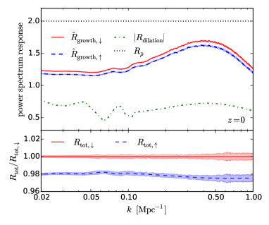
The top panel of Fig. 2 shows the various power spectrum responses at $z=0$, and the bottom panel shows the ratios of the total power spectrum response, $R_{\rm tot}$, to that of the sub-Jeans SU, $R_{{\rm tot},\downarrow}$. We find that the response is roughly 2% smaller in super-Jeans than in sub-Jeans SUs, and the distinction is statistically significant. Note also the small errors ($\sim 0.1\%$ at low-$k$ and $\sim 0.3\%$ at high-$k$) estimated from small-box SU simulations, demonstrating the power of the SU technique to precisely characterize the response down to arbitrarily small scales.

The fact that the growth response is smaller in super-Jeans than in sub-Jeans SUs can be understood qualitatively from Fig. 1. Normalized to a given observation redshift, $\delta_{m}$ in the super-Jeans limit is always smaller in the past than that in the sub-Jeans limit. Consequently, the super-Jeans SU is closer to the global universe along the growth history, and so the response is smaller.

This difference between super-Jeans and sub-Jeans scales produces an observable change in the local power spectrum, and so can in principle be used as a new probe of the sound speed of quintessence. In the real universe, the small-scale power spectrum responds to long modes of all scales, the difference of the responses in sub-Jeans and super-Jeans limit would thus appear as the scale-dependent squeezed-limit bispectrum for a fixed small-scale mode. However in quintessence models with initial curvature perturbations, the predicted amplitude for adiabatic quintessence fluctuations is proportional to $(1+w_{Q})$ (see Eq. (95) of Ref. Hu et al. (2016)) and so goes to zero as $w_{Q}\rightarrow-1$. More generally, this growth history dependence demonstrates that the nonlinear matter power spectrum cannot simply be a functional of the linear power spectrum at the same epoch as is commonly assumed in simple halo model and nonlinear fitting procedures (see also Ma (2007)).

IV.2 Perturbation Theory

Figure 3: The response of the separate universe growth function as a function of the global scale factor $a$ in the global universe for super-Jeans (red solid) and sub-Jeans (blue dashed) cases. Above the Jeans scale, the response to the same $\delta_{m}$ at $a$ is smaller than below.

Figure 4: Linear perturbation theory predictions for the growth responses compared with the measurements from the 20 small-box separate universe simulations at $z=3$ (top) and 0 (bottom). The red solid and blue dashed lines with shaded areas show the sub-Jeans and super-Jeans separate universes measurements as in Fig. 2, whereas the red dot-dashed and blue long-dashed lines show the corresponding linear perturbation theory predictions, i.e. Eqs. (19)–(20). Note that the range of $y$-axes is smaller in the top than in the bottom panel. Also the cusp feature at $k\sim 0.078~{}{\rm Mpc}^{-1}$ is a visual artifact due to binning, which we choose to be $\Delta k=2\pi/L$.

To better understand the growth responses quantitatively, we compute them in perturbation theory and check their agreement with the SU simulations at various redshifts. In perturbation theory, the effect can be modeled through the SU linear growth function $D_{W}$ as

$$R_{\rm growth}(k,a)=\frac{d\ln P(k,a)}{d\ln D_{W}(a)}\frac{d\ln D_{W}(a)}{d\delta_{m}(a)}\,.$$ (19)

In the linear regime $P(k,a)\approx P_{\rm lin}(k,a)\propto D_{W}^{2}(a)$ and so

$$\frac{d\ln P(k,a)}{d\ln D_{W}(a)}\approx 2\,.$$ (20)

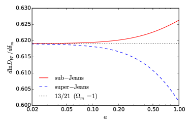
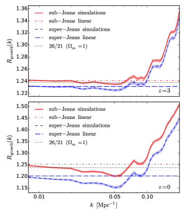
To determine the response of $D_{W}$ in Eq. (19), we solve Eq. (7) with the initial condition Eq. (10), and the result is shown in Fig. 3. It approaches the matter dominated ($\Omega_{m}=1$) limit $13/21$ at high redshift for both super-Jeans and sub-Jeans scale responses, and at low redshift is smaller in the super-Jeans case as expected from Fig. 1. In Fig. 4, we compare the measured power spectrum response in sub-Jeans and super-Jeans SUs to the corresponding linear perturbation theory predictions, i.e. Eqs. (19)–(20). We find that in both cases the linear perturbation theory agrees with the measured responses in the linear regime, i.e., at sufficiently low $k$ or high $z$.

Figure 5: Same as Fig. 4, but for the 1-loop predictions, i.e. Eq. (19) and Eq. (22).

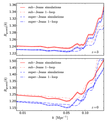
However, as we move to lower redshift as well as higher $k$, the measured responses become nonlinear and perturbation theory predictions deviate from SU simulation measurements. Unlike perturbation theory, the SU response calibration is not limited to large scales. On the other hand, we can understand the onset of nonlinearity in the simulations through higher order perturbation theory. The 1-loop power spectrum from standard perturbation theory is given by (see e.g. Ref. Jeong and Komatsu (2006))

$$P_{\rm 1-loop}(k,a)=P_{\rm lin}(k,a)+P_{22}(k,a)+2P_{13}(k,a)\,,$$ (21)

where the nonlinear corrections $P_{22}$ and $P_{13}$ are proportional to $D_{W}^{4}$ if $\Omega_{mW}(a_{W})/f_{W}^{2}(a_{W})\approx 1$. Therefore,

$$\frac{d\ln P_{\rm 1-loop}(k,a)}{d\ln D_{W}(a)}=2\left[1+\frac{P_{22}(k,a)+2P_{13}(k,a)}{P_{\rm 1-loop}(k,a)}\right]\,,$$ (22)

which now is a function of $k$. Note that in the global cosmology $\Omega_{m}/f^{2}=1.034$ at $z=3$ and 1.203 at $z=0$, and the standard perturbation theory should work better at $z=3$ than at $z=0$. Since the long-wavelength perturbation we consider is small ($|\delta_{\uparrow\downarrow 0}|=0.01$), the standard perturbation theory should work as well in both the sub-Jeans and super-Jeans SUs as the global universe.

In Fig. 5 we plot the 1-loop predictions in sub-Jeans (red dot-dashed) and super-Jeans (blue long-dashed). We find that the 1-loop predictions extend the agreement with the $N$-body measurement to smaller scales compared to the linear predictions. More precisely, the difference between the 1-loop model and the measurement at $z=3$ ($z=0$) is 1% (3%) at $k\sim 0.1~{}{\rm Mpc}^{-1}$ and 4% (6%) at $k\sim 0.2~{}{\rm Mpc}^{-1}$. At even smaller scale or lower redshift, the nonlinearity is too large to be modeled by the 1-loop perturbation theory. The SU simulation calibration technique itself is not limited in wavenumber and our $N$-body implementation is instead only limited by resolution as well as the lack of baryonic and astrophysical modeling in the deeply nonlinear regime.

IV.3 Position-Dependent Power Spectrum

The power spectrum response can also be tested in simulations and observed in surveys through the position-dependent power spectrum. As a simulation based test, it also serves to check the SU calibration of the power spectrum response deep into the nonlinear regime.

Specifically we compare the response measured from the small-box SU simulations to the squeezed-limit position-dependent power spectrum measured from the big-box simulations with the global cosmology (without a uniform long-wavelength density fluctuation). In the latter, we assume that the dark energy does not cluster with matter and so its position-dependent power spectrum should match the sub-Jeans SU prediction.

The procedure of measuring the position-dependent power spectrum is explained in detail in Chiang et al. (2014). In short, we first distribute the dark matter particles onto a $2048^{3}$ grid by the CIC density assignment scheme to construct the density fluctuation. We next divide the big-box simulations in each dimension by 8, so there are $N_{s}=512$ subvolumes in total with comoving side length of $L=350$ Mpc. In each subvolume centered at ${\mathbf{r}}_{L}$, we measure the local power spectrum as $\hat{P}(k,a|{\mathbf{r}}_{L})$ and the mean overdensity (with respect to the entire box) as $\hat{\bar{\delta}}_{m}({\mathbf{r}}_{L})$ and construct

$$\frac{\frac{1}{N_{s}}\sum_{{\mathbf{r}}_{L}}\hat{P}(k,a|{\mathbf{r}}_{L})\hat{\bar{\delta}}_{m}({\mathbf{r}}_{L})}{\left[\frac{1}{N_{s}}\sum_{{\mathbf{r}}_{L}}\hat{P}(k,a|{\mathbf{r}}_{L})\right]\left[\frac{1}{N_{s}}\sum_{{\mathbf{r}}_{L}}\hat{\bar{\delta}}_{m}^{2}({\mathbf{r}}_{L})\right]}\,,$$ (23)

where the summation is over the 512 subvolumes in one big-box realization. The correlation between $\hat{P}(k,a|{\mathbf{r}}_{L})$ and $\hat{\bar{\delta}}_{m}({\mathbf{r}}_{L})$ quantifies the integrated bispectrum, and in the squeezed limit where $k\ll 1/L$ the integrated bispectrum can be understood as the total response of the power spectrum to the long-wavelength overdensity.

Figure 6: Comparison of the squeezed-limit position-dependent power spectrum of big-box, global simulations (green dot-dashed), and the total power spectrum response of sub-Jeans (red solid) as well as super-Jeans (blue dashed) separate universe simulations at $z=0$. The shaded areas show the error on the mean. This figure summarizes our main power spectrum response results: the position-dependent power spectrum and the sub-Jeans power spectrum response agree significantly better than the difference in response across the Jeans scale confirming the scale dependence in this observable deep into the nonlinear regime.

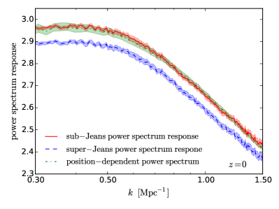
Fig. 6 shows the comparison at $z=0$ between the total power spectrum response from the previous section (red solid for sub-Jeans and blue dashed for super-Jeans cases) and the position-dependent power spectrum (green dot-dashed) averaged over the 20 realizations with its error. To reach the squeezed limit, we require $k\gtrsim 100/L\sim 0.3~{}{\rm Mpc}^{-1}$, and in this regime the agreement with the SU response is better than a percent. This agreement is significantly better than the difference between the super-Jeans and sub-Jeans power spectrum responses and thus verifies the SU calibration technique. With the SU technique tested into the nonlinear regime, we can apply these results to the super-Jeans case of the position-dependent power spectrum without the need for costly simulations that include dark energy clustering.

V Scale-Dependent Halo Bias

The SU simulations also calibrate the response of the halo mass function to a long-wavelength mode and hence the bias of the halo number density due to that mode. In Sec. V.1, we review the technique for measuring halo bias from SU simulations and show that in the quintessence model it acquires a scale dependence at the Jeans scale. In Sec. V.2, we test this response bias in the SU simulations against the clustering bias extracted from 40 small-box global simulations. We discuss the implications of scale dependence for the temporal nonlocality of halo bias and the observability of features in the halo power spectrum in Sec. V.3.

V.1 Response Bias

The linear density bias $b_{1}(M)$ of halos of mass $M$ can be defined as the response of the differential halo abundance $n_{\ln M}=dn/d\ln M$ to the long-wavelength mode

$$b_{1}(M)\equiv\frac{d\delta_{h}}{d\delta_{m}}=\frac{d\ln n_{\ln\!M}}{d\delta_{m}}\,,$$ (24)

which we call “response bias”. Thus by measuring the response of the halo mass function in the SU simulations we have a direct calibration of response bias Li et al. (2016); Lazeyras et al. (2016); Baldauf et al. (2015). Note that the derivative in Eq. (24) is evaluated at a fixed time, but will depend on the whole growth history of $\delta_{m}(a)$. This temporal nonlocality implies that response bias can be scale dependent if that growth history is also scale dependent. For quintessence, the SU simulations allow us to calibrate the bias above and below the Jeans length of quintessence without direct simulations of its clustering properties.

As discussed in Ref. Li et al. (2016), response bias largely reflects the change in the masses of halos due to the same local change in growth that affects the power spectrum. The enhanced growth in $\delta_{m}>0$ regions makes halos more massive locally than in their $\delta_{m}<0$ counterparts. Hence halos of a fixed mass are associated with the more abundant lower peaks in the initial density field in the former and the less abundant higher peaks in the latter. This also means that measuring the change in abundance of halos in fixed mass bins between the SU simulation pairs is an inefficient way to quantify response bias. Halos with small changes in mass across wide mass bins would register their response only when individual halos move across mass bins.

We instead adopt abundance matching as introduced in Ref. Li et al. (2016), which we now summarize. By finding the mass threshold above which the cumulative abundance is fixed, we largely eliminate the sampling noise from the discrete nature of halos.

Figure 7: Threshold mass shift as a response of varying $\delta_{m}$ at fixed cumulative abundance at $z=0$. The solid line and shaded region show the smoothed estimate and the bootstrap error.

Specifically for either the sub-Jeans or the super-Jeans case, we first combine halo catalogs of all realizations of the same $\delta_{m}$ in the small-box suite. The masses of the $i^{\rm th}$ most massive halo $M_{i}^{\pm}$ from the $\delta_{m}=\pm 0.01$ SU simulations determine the discrete threshold mass shift

$$s_{i}({\ln\!M}_{i})=\frac{{\ln\!M}_{i}^{+}-{\ln\!M}_{i}^{-}}{2|\delta_{m}|}\,,$$ (25)

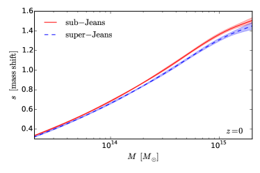
where $M_{i}$ is the geometric mean of $M_{i}^{+}$ and $M_{i}^{-}$. We then use the smoothing spline technique to estimate the ensemble average threshold mass shift $\hat{s}(\ln M)$ as well as the cumulative halo abundance above threshold mass $\hat{n}(\ln M)$. Fig. 7 shows the mass shift measured from 20 sub-Jeans and super-Jeans SU simulations at $z=0$ as a function of halo mass. We find that the mass shift due to varying $\delta_{m}$ is smaller above the Jeans scale, which reflects the fact that its growth history makes it closer to the global universe than below the Jeans scale.

The halo mass function follows as the derivative of the cumulative mass function $\hat{n}_{\ln\!M}=-d\hat{n}/d{\ln\!M}$. We can then estimate the Lagrangian halo bias above threshold mass $M$ as

$$\hat{\bar{b}}_{1}^{\textrm{L}}(M)=\frac{\hat{n}_{\ln\!M}(\ln M)\,\hat{s}(\ln M)}{\hat{n}(\ln M)}\,.$$ (26)

This quantity is the Lagrangian bias since the SU simulations are performed with the same comoving rather than physical volume. The dilation of the volume from the change in scale factors brings the cumulative Eulerian bias to

$$\hat{\bar{b}}_{1}(M)=1+\hat{\bar{b}}_{1}^{\textrm{L}}(M)\,.$$ (27)

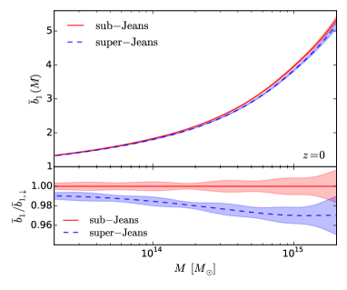
In Fig. 8 we compare the response bias on super-Jeans (blue dashed) and sub-Jeans (red solid) scales as a function of halo mass at $z=0$. The bias at a fixed mass is smaller in the super-Jeans case. Just like for the power spectrum response, above the Jeans scale for the same final $\delta_{m}$, the SU is closer to global at high redshift. Thus the change in growth and the consequent change in halo masses and abundances is smaller. We find that the mild mass dependence of the fractional difference between the super-Jeans and sub-Jeans response biases is due mainly to the dilation effect in Eq. (27), since that of the Lagrangian bias is fairly mass independent due to the similar shapes of the mass shift displayed in Fig. 7 (see also Fig. 11).

Figure 8: (Top) The $z=0$ response biases measured from 20 sub-Jeans (red solid) and super-Jeans (blue dashed) separate universe simulations. The lines and shaded areas show the smoothed estimate and the bootstrap error. (Bottom) The ratios of the response biases to that of the sub-Jeans response bias. The difference between the sub-Jeans and super-Jeans response biases, which indicates that the linear halo bias is scale dependent in the presence of the scale-dependent growth, is the second central result of our separate universe simulations.

V.2 Clustering Bias

To verify the SU calibration of halo bias through the mass function response, we can compare it to how linear halo bias is commonly measured from the two-point statistics, which we call clustering bias

$$\bar{b}_{1}(M)=\lim_{k\to 0}\frac{P_{hm}(k;M)}{P_{mm}(k)}\,,$$ (28)

where $P_{hm}$ is the cumulative halo number density cross power spectrum with the matter density. Where no confusion should arise, we omit the $M$ argument of the cumulative bias. Above the Jeans scale of quintessence, this approach would require simulations of quintessence clustering even for linear halo bias. Below the Jeans scale, we can test the equivalence of response and clustering bias with global simulations where quintessence enters only at the background level.

In order to extract the $k\rightarrow 0$ limit, we first compute

$$\bar{q}(k)=\frac{{P}_{hm}(k)}{P_{mm}(k)}\,,$$ (29)

for each of the 40 simulations of the global cosmology for a set of mass thresholds. Motivated by Ref. Assassi et al. (2014), we fit $\bar{q}(k)$ to the model

$$\bar{b}(k)=\bar{b}_{1}+\sum_{i=1}^{n}\bar{b}_{k^{2n}}k^{2n}\,,$$ (30)

where we treat $\bar{b}_{k^{2n}}$ as nuisance parameters that absorb the loop corrections in the large-scale limit. We then get the best-fit bias parameters by minimizing

$$\chi^{2}=\sum_{k}^{k_{\rm max}}\frac{[\bar{q}(k)-\bar{b}(k)]^{2}}{\sigma^{2}[\bar{q}(k)]}\,,$$ (31)

where $\sigma^{2}[\bar{q}(k)]$ is the variance of $\bar{q}(k)$ measured from 40 global small-box simulations.

To ensure the robustness of the fitted clustering bias, especially as compared with the small predicted difference between sub-Jeans and super-Jeans response biases, we examine the bias models with $n=0$, 1, and 2 for various $k_{\rm max}$. We seek consistent result for different bias models (different $n$) and $k_{\rm max}$. The general principle is that the larger the $k_{\rm max}$, the larger the $n$ required to account for the nonlinearity and to avoid underfitting. Conversely, for models with $n>0$ $k_{\rm max}$ cannot be too small or the fit would suffer from overfitting.

With each bias model and $k_{\rm max}$, we visually inspect its goodness of fit to $\bar{q}(k)$ for various threshold halo masses. We find that across two decades in halo mass ($2\times 10^{13}-2\times 10^{15}\,M_{\odot}$), the bias models of $n=0$, 1, and 2 with the biases fitted to $k_{\rm max}=0.014-0.028\,{\rm Mpc}^{-1}$, $0.042-0.049\,{\rm Mpc}^{-1}$, and $0.056-0.07\,{\rm Mpc}^{-1}$ are in agreement with the mean $\bar{q}(k)$, and the agreement even extends to $k>k_{\rm max}$. This shows that the fit is free from overfitting and underfitting problems. For a given halo mass, the best-fit clustering bias varies up to 0.2%, 0.5%, and 2% among different $n$ and $k_{\rm max}$ at $2\times 10^{13}\,M_{\odot}$, $2\times 10^{14}\,M_{\odot}$, and $2\times 10^{15}\,M_{\odot}$, respectively. Given the fact that the clustering bias is stable for various bias models and fitting range, we conclude that systematic error due to $n$ and $k_{\rm max}$ is at most comparable to our statistical error, and is the largest at the high-mass end at which the statistical error is also large.

Figure 9: The ratios of the linear biases to that of the sub-Jeans response bias at $z=0$. The red solid and blue dashed lines show the sub-Jeans and super-Jeans response biases measured from 20 separate universe simulations, whereas the green dot-dashed line shows the clustering bias measured from 40 global simulations. The error of the clustering bias is measured from the scatter of the 40 simulations. This figure summarizes the main results on halo bias: the agreement between the clustering bias measured from global simulations and the sub-Jeans response bias verifies the observable difference in halo bias across the Jeans scale inferred from the separate universe simulations.

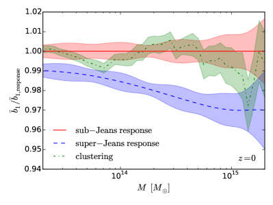
In Fig. 9 we shows our fiducial results of the clustering bias measurement for the quadratic model ($n=1$) with $k_{\rm max}=0.49\,{\rm Mpc}^{-1}$, which gives the smallest statistical errors. We find that the clustering bias is in good agreement with the sub-Jeans response bias across two decades in halo mass, confirming the validity of the SU technique. This agreement is substantially better than the difference between the super-Jeans and sub-Jeans response bias at low- and mid-mass regime, even after including the systematic differences between the fitting techniques.

To further test robustness of the scale-dependent bias result, we also try the halo finding algorithm provided in Ref. Li et al. (2016), another spherical overdensity finder similar to that in Ref. Tinker et al. (2008). We find that the clustering bias is statistically in equally good agreement with the sub-Jeans response as well.

With this verification of the SU calibration of halo bias, our results represent the first simulation confirmation of scale-dependent halo bias from scale-dependent growth. A related effect on the void bias has been measured in the simulations with cold dark matter and massive neutrinos Banerjee and Dalal (2016).

Figure 10: Fractional difference or “step” across the Jeans scale in the matter (red solid, Eq. (32)) versus the halo (blue dashed, Eq. (33)) power spectra. The step in the halo power spectrum is reduced by approximately a factor of 2 compared with the matter power spectrum at high mass where the Lagrangian bias contribution dominates. Bias prescriptions which assume locality at either the observed or initial redshift predict the same step or zero step respectively at high masses.

V.3 Scale-Dependent Bias and Power Spectra

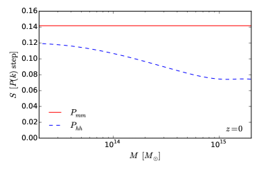
Since the halo bias is smaller above versus below the Jeans scale of quintessence, its scale dependence counters the growth rate effects in the matter power spectrum. This is especially true at high masses where the Lagrangian bias dominates. The change in the linear growth function above $(D^{\uparrow})$ versus below $(D^{\downarrow})$ the Jeans scale leads to a step in the linear matter power spectrum of approximately

$$S_{mm}\equiv 2\frac{D^{\uparrow}-D^{\downarrow}}{D^{\downarrow}}\,,$$ (32)

whereas the step in the cumulative halo power spectrum is

$$S_{hh}\equiv 2\frac{D^{\uparrow}\bar{b}_{1}^{\uparrow}-D^{\downarrow}\bar{b}_{1}^{\downarrow}}{D^{\downarrow}\bar{b}_{1}^{\downarrow}}\,.$$ (33)

In Fig. 10, we show the amplitude of these steps as a function of mass. At the high mass end the halo power spectrum has half the step amplitude of the matter power spectrum.

This result not only confirms that scale-dependent linear growth leads to scale-dependent bias, but it does so in a way that both reduces the observability of features in the halo power spectrum LoVerde (2014a) and violates principles that underlie simple models for bias. It is commonly assumed that the statistics of halos at any observation epoch is determined solely by the statistics of the linear density field at a single epoch, and hence bias is scale-free with respect to the matter power spectrum at that epoch. For models with scale-dependent growth, this epoch is commonly taken to be the initial epoch for models where the growth becomes scale-free during matter domination Parfrey et al. (2011).

For example in the excursion set, Lagrangian bias is given by the conditional probability that the initial density field crosses some barrier at a smoothing scale $R_{S}$ corresponding to the mass $M$ at the background density given that it takes the value $\delta_{m}$ at some larger scale $R_{L}$ via a random walk between the two. For our quintessence case where these scales are arbitrarily well separated by our SU assumption, the lack of correlation in the Gaussian random initial conditions between these scales means that halo bias is local in the initial density field. Specifically, the conditional probability cannot depend on steps in the random walk with $R>R_{L}$, and hence whether $\delta_{m}$ was achieved from super-Jeans or sub-Jeans scale fluctuations. This holds regardless of the shape of the barrier, its dependence on the redshift of observation, or some putative intermediate epoch of halo formation. As a result, Lagrangian halo bias should be scale-free with respect to the matter power spectrum at the initial epoch.

As emphasized in Ref. Parfrey et al. (2011), even if the Lagrangian bias is scale-free with respect to the initial power spectrum, it becomes scale dependent with respect to the matter power spectrum at the observation epoch. This effect is solely due to the scale-dependent growth in the latter, and hence the scale dependence takes a simple and specific form $b_{1}^{L\uparrow}=(D^{\downarrow}/D^{\uparrow})b_{1}^{L\downarrow}$. In Appendix A, we review this construction in more detail. In the quintessence model this means that the step in the halo power spectrum should be absent when the Lagrangian bias dominates $\lim_{M\rightarrow\infty}S_{hh}=0$ (see Eq. (33)). Our results significantly violate this prediction.

Similarly models of halo bias that rely on a universal mass function ansatz, characterize the bias as its derivative with respect to $\delta_{m}$ at the observation epoch. If this derivative depends only on the local density field $\delta_{m}$ at the observation epoch, for example by assuming a change in the spherical collapse threshold $d\delta_{c}/d\delta_{m}=-1$ (see Appendix A), then the Lagrangian bias would be local and hence scale-free with respect to the matter power spectrum at the observation epoch. Our results for scale-dependent bias directly violate this prediction and are essentially half-way between these two extreme models. We find that halo bias is nonlocal in time and cannot be characterized by the statistics of the density field at a single epoch, initial or observed when there is scale-dependent linear growth.

In Appendix A, we show that encapsulating the dependence on the growth history of $\delta_{m}(a)$ through its impact on the spherical collapse threshold at the observation epoch and assuming a universal mass function characterizes the quintessence SU simulation results better than either of these simplistic models. However given the assumptions underlying this type of modeling, its validity in other contexts should be tested directly in simulations.

VI Discussion

Quintessence dark energy provides an arena to explore the response of small-scale observables to the amplitude, scale, and growth history of long-wavelength fluctuations with the separate universe technique. In the presence of quintessence fluctuations, the growth of long-wavelength fluctuations differ above and below its Jeans scale. We verify that even below the Jeans scale, where a naive separate universe picture does not strictly apply because the local curvature evolves due to non-gravitational forces which keep the quintessence smooth, the response of small-scale observables can still be accurately modeled by a modified expansion history alone. One implication of this finding is that halo bias is not directly a response of halo number density to the local curvature, but rather to the local expansion history.

Using this technique, we show that in the presence of the scale-dependent growth, the local power spectrum and halo mass function acquire a dependence on the scale of the long-wavelength mode. Equivalently, the squeezed bispectrum and halo bias become scale dependent. To our knowledge, our results are the first verification of scale-dependent bias from scale-dependent growth using simulations. Moreover they violate predictions of models where bias is effectively local in the density field at a single epoch, initial or observed, and show that halo bias is temporally nonlocal. Likewise the nonlinear matter power spectrum cannot simply be a function of the linear power spectrum at the same epoch.

Specifically, we use the separate universe (SU) technique to perform $N$-body simulations in the sub-Jeans and super-Jeans SUs. By differencing pairs of overdense and underdense SU simulations with the same Gaussian realizations of initial phases, much of the sample variance is canceled, and so we can precisely characterize the responses of the power spectrum (which is equivalent to the squeezed-limit bispectrum) and the halo mass function (which gives the linear halo bias) to the long-wavelength matter fluctuation.

We validate the SU approach by comparing to perturbation theory predictions for the power spectrum response in both the super-Jeans and sub-Jeans limits (see Figs. 4-5). Since it is the sub-Jeans limit where the SU technique might naively fail, we further test it with direct simulations that possess long-wavelength matter modes in big-box simulations with smooth dark energy. We find that the squeezed-limit position-dependent power spectrum measured from the big-box simulations agrees with the power spectrum response to the resolution limit $k\sim 1\,{\rm Mpc}^{-1}$. Similarly, the clustering bias is statistically consistent with the response bias across two decades in halo mass ($\sim\!10^{13}\!-\!10^{15}\,M_{\odot}$). Thus, with the SU technique verified into the nonlinear regime, we can robustly assess the scale-dependence of the power spectrum and halo density responses across the Jeans scale without costly simulations that include quintessence clustering.

We show that for both responses there is a statistically significant distinction between sub-Jeans and super-Jeans SUs at $z=0$. More precisely, the power spectrum response in the super-Jeans SU is roughly 2% smaller than that in the sub-Jeans SU for $k\lesssim 1\,{\rm Mpc}^{-1}$; the halo bias in the super-Jeans SU is roughly 1% and 3% smaller than that in the sub-Jeans SU for halo mass of $2\times 10^{13}$ and $2\times 10^{15}~{}M_{\odot}$ respectively. The fact that the response is smaller in the super-Jeans SU is because quintessence enhances the growth of matter fluctuations there, and so the super-Jeans overdensity was smaller in the past. These key SU results, along with the comparison to the global simulations, are summarized in Fig. 6 and Fig. 9.

More generally, this dependence on the growth history of the long wavelength fluctuation indicates that the response of small scale observables is nonlocal in time. In particular, the statistically significant difference between sub-Jeans and super-Jeans response biases measured in our SU simulations falsifies the standard Lagrangian picture where the statistics of halos at any observation epoch is determined solely by the statistics of the linear density field at a single epoch.

These effects are in principle important for interpreting observational tests of quintessence clustering from galaxy surveys and their cross correlation with the CMB (e.g. Bean and Dore (2004); Hu and Scranton (2004)). In particular, the step feature in the halo power spectrum is smaller by up to a factor of 2 compared with the matter. However these corrections, while significant relative to the clustering effects on the matter power spectrum itself, are small in an absolute sense for observationally viable dark energy equations of state (i.e. $w_{Q}\approx-1$) in the absence of quintessence isocurvature fluctuations Gordon and Hu (2004); Hu et al. (2016).

On the other hand, the same technique which has been validated here using quintessence, can be applied to more observationally viable cosmological models, such as those with massive neutrinos. Massive neutrinos cluster with dark matter on large scales, but their free streaming sets an effective Jeans scale. This would generate not only a feature in the two-point function of the total matter Lesgourgues and Pastor (2006), but also influence the high-order statistics Shoji and Komatsu (2009); Blas et al. (2014); Führer and Wong (2015); Levi and Vlah (2016) as well as the halo bias LoVerde (2014a). We intend to apply the SU technique to study how massive neutrinos affect the small-scale structure formation in a future work.

Appendix A Bias model comparisons

Here we make brief comparisons with formalisms for scale-dependent halo bias in the recent literature. Analytic models for scale-dependent bias arising from scale-dependent growth exist and have been applied to modified gravity Hui and Parfrey (2008); Parfrey et al. (2011) and to massive neutrino cosmologies LoVerde (2014a, 2016). Both formalisms can be applied to the quintessence model studied in this paper.

A.1 PHS11: Excursion set on the initial density field

Parfrey, Hui, and Sheth Parfrey et al. (2011) (hereafter PHS11) develop the theory of excursion sets for a cosmology with a scale-dependent linear growth function $D(z;k)$ caused by modified gravity associated with the late-time accelerated expansion of the universe. We can equally well apply their construction to the quintessence model.

In the PHS11 model, halos are identified by performing a barrier-crossing calculation on the initial density field, $\delta_{i}$ at some redshift in the matter dominated era, $z_{i}$, before the linear growth of the matter field becomes scale dependent. In the PHS11 model the scale-dependent evolution of density perturbations (i) causes the barrier to be scale-dependent (ii) induces scale-dependent Lagrangian bias from the scale-dependent mapping between the statistics of the density field at $z_{i}$ and those at a later redshift $z$.

As discussed in Sec. V.3, for the quintessence model a scale-dependent barrier can change the mass dependence of the bias but cannot introduce a scale dependence. Unlike the modified gravity model of PHS11, we assume in the quintessence model an arbitrarily large separation of scales involved in the barrier crossing and the long-wavelength modes enforced by the SU approximation. In addition PHS11 find that in their model the approximation of a flat barrier (constant with scale) is good. Their model for the Lagrangian bias observed at redshift $z$ is

$$b_{1}^{L}(z;k)=\frac{D(z_{i};k)}{D(z;k)}b_{1}^{L}(z_{i})\,,$$ (34)

where the Lagrangian bias at $z_{i}$ is independent of $k$ and for a flat barrier $\delta_{c}$ is explicitly

$$b_{1}^{L}(z_{i})=\left[\frac{\delta_{c}^{2}}{\sigma^{2}(z_{i})}-1\right]\frac{1}{\delta_{c}}\,.$$ (35)

The barrier height is typically derived from the spherical collapse model with $\delta_{c}(z_{\rm form})$ as the critical value of an initial overdensity that will collapse to “form” a halo by $z_{\rm form}$. The bias in PHS11 is a function of both the observed $z$ and $z_{\rm form}$ and the bias at $z=z_{\rm form}$ can be scale dependent. While these distinctions can change the prediction for the value of the bias as a function of mass, they do not introduce an additional dependence on $k$.

The PHS11 flat-barrier expression for the bias in Eq. (34) has a particularly clean interpretation: halos have scale-independent Lagrangian bias with respect to the initial matter power spectrum

$$P^{L}_{hh}(k;z)\> \equiv\left[b_{1}^{L}(z;k)\right]^{2}P_{mm}(k;z)$$ (36)

$$=[b_{1}^{L}(z_{i})]^{2}P_{mm}(k;z_{i})\,.$$

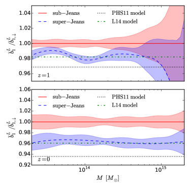
The scale dependence of the Lagrangian halo bias arises entirely from the evolution of the matter power spectrum leaving no scale in the Lagrangian halo power spectrum. We test this concrete and robust prediction in the main text and find that the quintessence model significantly violates this expectation. This point is further illustrated in Fig. 11, which compares the fractional change in the Lagrangian bias measured in our simulations to the prediction in Eq. (34). The flaw in this approach, that bias is local in the initial density field, can be ameliorated by making the barrier explicitly dependent on the random walk on larger scales. This is discussed in the next section.

Figure 11: Ratio of the super-Jeans to sub-Jeans scale Lagrangian bias factors at $z=1$ (top) and $z=0$ (bottom) measured from separate universe simulations in comparison with the two models, PHS11 in Eq. (34) and L14 in Eq. (43), discussed in this Appendix. Oscillations are mainly due to spline smoothing. Increasing the number of knots gives flatter curves with larger errors but consistent averages. Large errors at $z=1$ for $M\gtrsim 10^{15}M_{\odot}$ are due to the lack of high redshift massive halos. The PHS11 model predictions rely on the standard assumption that Lagrangian bias is scale-independent with respect to the initial density field, and our simulations rule this out.

A.2 L14: Peak background split on a universal mass function

A related but conceptually distinct calculation for scale-dependent bias, developed for massive neutrinos, is given in LoVerde LoVerde (2014a) (hereafter “L14”). The L14 model makes the assumption that the halo abundance at $z$ is given by a universal function of $\nu\equiv\delta_{c}(z;k)/\sigma(M,z)$. Here $\delta_{c}(z;k)$ is associated with the spherical collapse threshold at $z$ computed in the presence of the long-wavelength or “background” mode $\delta_{m}(k)$ and $\sigma(M,z)$ is the rms of the linear density field smoothed by a top-hat in $R$ that encloses $M$ at the background density. Specifically, the mass function takes the familiar form

$$n_{\ln M}(M,z)=\frac{\bar{\rho}_{m}}{M}\frac{d\nu}{d\ln M}f(\nu)\,,$$ (37)

and the Lagrangian bias is given by

$$b^{L}_{1}(M,z)\equiv\frac{\partial\ln n_{\ln M}}{\partial\delta_{m}}=\frac{d\ln n_{\ln M}}{d\nu}\frac{1}{\sigma(M,z)}\frac{d\delta_{c}}{d\delta_{m}}\,,$$ (38)

where ${d\delta_{c}}/{d\delta_{m}}$ is the response of the collapse threshold at $z$ to the entire growth history of a long-wavelength mode which reaches $\delta_{m}$ at $z$ in a manner that depends on $k$. The partial derivative denotes the fact that it is at fixed comoving volume and does not account for the dilation induced by $\delta_{m}$. In this way, the model differs fundamentally from ones that assume halo bias is local in the density field at a single epoch. On the other hand the association of the observed redshift $z$ with the collapse or formation redshift of all halos is ad hoc since real halos continually grow in mass and merge with each other. Predictions would differ substantially if for example this redshift were instead associated with the last major merger of a halo.

The collapse threshold $\delta_{c}(z)$ is computed by numerically solving for the evolution of a top-hat density perturbation of size $R$ enclosing mass $M=4\pi R^{3}{\bar{\rho}_{m}}/3$ in the presence of the long-wavelength mode and its whole evolutionary history, $\delta_{m}(z)$. If the components other than CDM (here quintessence) do not cluster on the scale of the top-hat, the evolution of the radius $R$ is given by

$$\ddot{R}=\> -\frac{4\pi G}{3}\sum_{J\neq\rm CDM}\left[\bar{\rho}_{J}(t)+3\bar{p}_{J}(t)+\delta\rho_{J}(t)+3\delta p_{J}(t)\right]R$$

$$-\frac{GM(<R)}{R^{2}}\,,$$ (39)

where $\delta\rho_{J}$ and $\delta p_{J}$ are the long-wavelength perturbations in the non-CDM components that may exist along with $\delta_{m}(z)$. Eq. (39) is solved with the initial conditions

$$R_{i}\> =\frac{3M}{(4\pi{\bar{\rho}_{m}})^{1/3}}\left[1-\frac{\delta_{i}+\delta_{m}(z_{i})}{3}\right]\,,$$

$$\dot{R}_{i}\> =H_{i}R_{i}\left[1-\frac{\dot{\delta}_{i}+\dot{\delta}_{m}(z_{i})}{3H_{i}}\right]\,,$$ (40)

where $\delta_{i}$ is the initial amplitude of the perturbation on scale $R$ and $\delta_{m}(z_{i})$ is the initial amplitude of the long-wavelength mode. The collapse threshold is the critical value of $\delta_{i}$ needed to collapse ($R\rightarrow 0$) at $z$ linearly extrapolated to $z$

$$\delta_{c}(z)=\frac{D^{\downarrow}(z)}{D^{\downarrow}(z_{i})}\delta_{i}\,.$$ (41)

Here we have assumed that the top-hat radius is always below the Jeans scale. The response of the collapse threshold to the long-wavelength mode is

$$\frac{d\delta_{c}}{d\delta_{m}}(z)=\frac{\delta_{c}(z|\delta_{m})-\delta_{c}(z)}{\delta_{m}(z)}\,.$$ (42)

For further details see LoVerde (2014a, b).

Note that for $z_{i}$ deep in the matter dominated era the linear growth rates of $\delta_{i}$ and $\delta_{m}(z_{i})$ are the same both above and below the Jeans scale. Below the Jeans scale, the linear evolution of the long-wavelength mode is entirely the same as the linear evolution of the mode on scale $R$, and we recover the usual result ${d\delta_{c}}/{d\delta_{m}}=-1$ that makes bias scale-free below the Jeans scale at the observation epoch.

Above the Jeans scale, this relation is no longer true since the long-wavelength mode grows faster than the linear evolution of the mode on scale $R$. The prediction for the difference between the Lagrangian bias factors on sub-Jeans ($\downarrow$) and super-Jeans ($\uparrow$) Jeans scales is then

$$\frac{b^{L\uparrow}_{1}-b^{L\downarrow}_{1}}{b^{L\downarrow}_{1}}=-\left(\frac{d\delta_{c}}{d\delta_{\uparrow}}+1\right)\,.$$ (43)

In Fig. 11, we compare this prediction to the separate universe response bias at $z=0$ and $z=1$. These predictions better capture the temporal nonlocality of halo bias than the PHS11 model. Had we assumed, contrary to fact, that the change in the collapse threshold is determined at the initial epoch $\delta_{i}(\delta_{m})=\delta_{i}-\delta_{m}(z_{i})$ then $d\delta_{c}/d\delta_{m}(z)=-D^{\downarrow}(z)/D^{\uparrow}(z)$ and we would recover the PHS11 prediction. Instead the L14 model assumes a universal mass function in the peak height $\nu$ of the spherical collapse threshold at the observation epoch.

References

- Bernardeau et al. (2002) F. Bernardeau, S. Colombi, E. Gaztanaga, and R. Scoccimarro, Phys. Rept. 367, 1 (2002), arXiv:astro-ph/0112551 [astro-ph] .
- Takada and Hu (2013) M. Takada and W. Hu, Phys. Rev. D87, 123504 (2013), arXiv:1302.6994 [astro-ph.CO] .
- Li et al. (2014a) Y. Li, W. Hu, and M. Takada, Phys. Rev. D90, 103530 (2014a), arXiv:1408.1081 [astro-ph.CO] .
- Chiang et al. (2014) C.-T. Chiang, C. Wagner, F. Schmidt, and E. Komatsu, JCAP 1405, 048 (2014), arXiv:1403.3411 [astro-ph.CO] .
- Chiang et al. (2015) C.-T. Chiang, C. Wagner, A. G. Sánchez, F. Schmidt, and E. Komatsu, JCAP 1509, 028 (2015), arXiv:1504.03322 [astro-ph.CO] .
- Mo and White (1996) H. J. Mo and S. D. M. White, Mon. Not. Roy. Astron. Soc. 282, 347 (1996), arXiv:astro-ph/9512127 [astro-ph] .
- Seljak (2012) U. Seljak, JCAP 1203, 004 (2012), arXiv:1201.0594 [astro-ph.CO] .
- Barrow and Saich (1993) J. D. Barrow and P. Saich, Mon. Not. Roy. Astron. Soc. 262, 717 (1993).
- Baldauf et al. (2011) T. Baldauf, U. Seljak, L. Senatore, and M. Zaldarriaga, JCAP 1110, 031 (2011), arXiv:1106.5507 [astro-ph.CO] .
- Sherwin and Zaldarriaga (2012) B. D. Sherwin and M. Zaldarriaga, Phys. Rev. D85, 103523 (2012), arXiv:1202.3998 [astro-ph.CO] .
- Sirko (2005) E. Sirko, Astrophys. J. 634, 728 (2005), arXiv:astro-ph/0503106 [astro-ph] .
- Gnedin et al. (2011) N. Y. Gnedin, A. V. Kravtsov, and D. H. Rudd, Astrophys. J. Suppl. 194, 46 (2011), arXiv:1104.1428 [astro-ph.CO] .
- Li et al. (2014b) Y. Li, W. Hu, and M. Takada, Phys. Rev. D89, 083519 (2014b), arXiv:1401.0385 [astro-ph.CO] .
- Wagner et al. (2015a) C. Wagner, F. Schmidt, C.-T. Chiang, and E. Komatsu, Mon. Not. Roy. Astron. Soc. 448, L11 (2015a), arXiv:1409.6294 [astro-ph.CO] .
- Wagner et al. (2015b) C. Wagner, F. Schmidt, C.-T. Chiang, and E. Komatsu, JCAP 1508, 042 (2015b), arXiv:1503.03487 [astro-ph.CO] .
- Li et al. (2016) Y. Li, W. Hu, and M. Takada, Phys. Rev. D93, 063507 (2016), arXiv:1511.01454 [astro-ph.CO] .
- Lazeyras et al. (2016) T. Lazeyras, C. Wagner, T. Baldauf, and F. Schmidt, JCAP 1602, 018 (2016), arXiv:1511.01096 [astro-ph.CO] .
- Baldauf et al. (2015) T. Baldauf, U. Seljak, L. Senatore, and M. Zaldarriaga, (2015), arXiv:1511.01465 [astro-ph.CO] .
- McDonald (2003) P. McDonald, Astrophys. J. 585, 34 (2003), arXiv:astro-ph/0108064 [astro-ph] .
- Cieplak and Slosar (2016) A. M. Cieplak and A. Slosar, JCAP 1603, 016 (2016), arXiv:1509.07875 [astro-ph.CO] .
- Ma (2007) Z.-M. Ma, Astrophys. J. 665, 887 (2007), arXiv:astro-ph/0610213 [astro-ph] .
- Senatore (2015) L. Senatore, JCAP 1511, 007 (2015), arXiv:1406.7843 [astro-ph.CO] .
- LoVerde (2014a) M. LoVerde, Phys. Rev. D90, 083530 (2014a), arXiv:1405.4855 [astro-ph.CO] .
- Dai et al. (2015) L. Dai, E. Pajer, and F. Schmidt, JCAP 1510, 059 (2015), arXiv:1504.00351 [astro-ph.CO] .
- Hu et al. (2016) W. Hu, C.-T. Chiang, Y. Li, and M. LoVerde, Phys. Rev. D94, 023002 (2016), arXiv:1605.01412 [astro-ph.CO] .
- Lewis et al. (2000) A. Lewis, A. Challinor, and A. Lasenby, Astrophys. J. 538, 473 (2000), arXiv:astro-ph/9911177 [astro-ph] .
- Howlett et al. (2012) C. Howlett, A. Lewis, A. Hall, and A. Challinor, JCAP 1204, 027 (2012), arXiv:1201.3654 [astro-ph.CO] .
- Crocce et al. (2006) M. Crocce, S. Pueblas, and R. Scoccimarro, Mon. Not. Roy. Astron. Soc. 373, 369 (2006), arXiv:astro-ph/0606505 [astro-ph] .
- (29) R. Scoccimarro, “2LPTIC,” http://cosmo.nyu.edu/roman/2LPT.
- Springel (2005) V. Springel, Mon. Not. Roy. Astron. Soc. 364, 1105 (2005), arXiv:astro-ph/0505010 [astro-ph] .
- Knollmann and Knebe (2009) S. R. Knollmann and A. Knebe, Astrophys. J. Suppl. 182, 608 (2009), arXiv:0904.3662 [astro-ph.CO] .
- Gill et al. (2004) S. P. D. Gill, A. Knebe, and B. K. Gibson, Mon. Not. Roy. Astron. Soc. 351, 399 (2004), arXiv:astro-ph/0404258 [astro-ph] .
- (33) “FFTW,” http://www.fftw.org.
- Jeong and Komatsu (2006) D. Jeong and E. Komatsu, Astrophys. J. 651, 619 (2006), arXiv:astro-ph/0604075 [astro-ph] .
- Assassi et al. (2014) V. Assassi, D. Baumann, D. Green, and M. Zaldarriaga, JCAP 1408, 056 (2014), arXiv:1402.5916 [astro-ph.CO] .
- Tinker et al. (2008) J. L. Tinker, A. V. Kravtsov, A. Klypin, K. Abazajian, M. S. Warren, G. Yepes, S. Gottlober, and D. E. Holz, Astrophys. J. 688, 709 (2008), arXiv:0803.2706 [astro-ph] .
- Banerjee and Dalal (2016) A. Banerjee and N. Dalal, (2016), arXiv:1606.06167 [astro-ph.CO] .
- Parfrey et al. (2011) K. Parfrey, L. Hui, and R. K. Sheth, Phys. Rev. D83, 063511 (2011), arXiv:1012.1335 [astro-ph.CO] .
- Bean and Dore (2004) R. Bean and O. Dore, Phys. Rev. D69, 083503 (2004), arXiv:astro-ph/0307100 [astro-ph] .
- Hu and Scranton (2004) W. Hu and R. Scranton, Phys. Rev. D70, 123002 (2004), arXiv:astro-ph/0408456 [astro-ph] .
- Gordon and Hu (2004) C. Gordon and W. Hu, Phys. Rev. D70, 083003 (2004), arXiv:astro-ph/0406496 [astro-ph] .
- Lesgourgues and Pastor (2006) J. Lesgourgues and S. Pastor, Phys. Rept. 429, 307 (2006), arXiv:astro-ph/0603494 [astro-ph] .
- Shoji and Komatsu (2009) M. Shoji and E. Komatsu, Astrophys. J. 700, 705 (2009), arXiv:0903.2669 [astro-ph.CO] .
- Blas et al. (2014) D. Blas, M. Garny, T. Konstandin, and J. Lesgourgues, JCAP 1411, 039 (2014), arXiv:1408.2995 [astro-ph.CO] .
- Führer and Wong (2015) F. Führer and Y. Y. Y. Wong, JCAP 1503, 046 (2015), arXiv:1412.2764 [astro-ph.CO] .
- Levi and Vlah (2016) M. Levi and Z. Vlah, (2016), arXiv:1605.09417 [astro-ph.CO] .
- Hui and Parfrey (2008) L. Hui and K. P. Parfrey, Phys. Rev. D77, 043527 (2008), arXiv:0712.1162 [astro-ph] .
- LoVerde (2016) M. LoVerde, Phys. Rev. D93, 103526 (2016), arXiv:1602.08108 [astro-ph.CO] .
- LoVerde (2014b) M. LoVerde, Phys. Rev. D90, 083518 (2014b), arXiv:1405.4858 [astro-ph.CO] .