Quantum metrology with nonclassical states of atomic ensembles
Abstract
Quantum technologies exploit entanglement to revolutionize computing, measurements, and communications. This has stimulated the research in different areas of physics to engineer and manipulate fragile many-particle entangled states. Progress has been particularly rapid for atoms. Thanks to the large and tunable nonlinearities and the well developed techniques for trapping, controlling and counting, many groundbreaking experiments have demonstrated the generation of entangled states of trapped ions, cold and ultracold gases of neutral atoms. Moreover, atoms can couple strongly to external forces and light fields, which makes them ideal for ultra-precise sensing and time keeping. All these factors call for generating non-classical atomic states designed for phase estimation in atomic clocks and atom interferometers, exploiting many-body entanglement to increase the sensitivity of precision measurements. The goal of this article is to review and illustrate the theory and the experiments with atomic ensembles that have demonstrated many-particle entanglement and quantum-enhanced metrology.
pacs:
03.67.Bg, 03.67.Mn, 03.75.Dg, 03.75.Gg, 06.20.Dk, 42.50.DvI Introduction
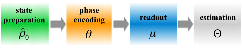
The precise measurement of physical quantities such as the strength of a field, a force, or time, plays a crucial role in the advancement of physics. Precision measurements are very often obtained by mapping the physical quantity to a phase shift that can be determined using interferometric techniques. Phase estimation is thus a unifying framework for precision measurements. It follows the general scheme outlined in Fig. 1: a probe state of particles is prepared, acquires a phase shift , and is finally detected. From the measurement outcome an estimate of the phase shift is obtained. This conceptually simple scheme is common to all interferometric sensors: from gravitational wave detectors to atomic clocks, gyroscopes, and gravimeters, just to name a few. The goal is to estimate with the smallest possible uncertainty given finite resources such as time and number of particles. The noise that determines can be of a technical (classical) or fundamental (quantum) nature Helstrom (1976); Braunstein and Caves (1994); Holevo (1982). Current two-mode atomic sensors are limited by the so-called standard quantum limit, , inherent in probes using a finite number of uncorrelated Giovannetti et al. (2006) or classically-correlated Pezzè and Smerzi (2009) particles. Yet, the standard quantum limit is not fundamental Caves (1981); Yurke et al. (1986); Bondurant and Shapiro (1984). Quantum-enhanced metrology studies how to exploit quantum resources, such as squeezing and entanglement, to overcome this classical bound Giovannetti et al. (2011, 2004); Pezzè and Smerzi (2014); Tóth and Apellaniz (2014). Research on quantum metrology with atomic ensembles also sheds new light on fundamental questions about many-particle entanglement Amico et al. (2008); Gühne and Tóth (2009); Horodecki et al. (2009) and related concepts, such as Einstein-Podolsky-Rosen correlations Reid et al. (2009) and Bell nonlocality Brunner et al. (2014).
Since the systems of interest for quantum metrology often contain thousands or even millions of particles, it is generally not possible to address, detect, and manipulate all particles individually. Moreover, the finite number of measurements limits the possibility to fully reconstruct the generated quantum states. These limitations call for conceptually new approaches to the characterization of entanglement that rely on a finite number of coarse-grained measurements. In fact, many schemes for quantum metrology require only collective manipulations and measurements on the entire atomic ensemble. Still, the results of such measurements allow one to draw many interesting conclusions about the underlying quantum correlations between the particles.
I.1 Entanglement and interferometric sensitivity enhancement: exemplary cases
We illustrate here how the standard quantum limit arises in interferometry and how it can be overcome using entanglement. Consider a Ramsey interferometer sequence Ramsey (1963) between two quantum states and , as used e.g. in an atomic clock, see Sec. II. Let us discuss first the case of a single atom initially prepared in the probe state . The atom is transformed to by a resonant -pulse corresponding to the first beam splitter of the interferometer. During the subsequent interrogation time, and acquire a relative phase , such that the state evolves to . The phase encodes the quantity to be measured, such as frequency in the case of an atomic clock or the strength of an external field in the case of an atom interferometer. To convert it into an observable population difference, a second resonant -pulse (the second beam splitter) is applied so that the final state is . The phase can now be estimated, for instance, by measuring the population difference between the two states. In this simple example the interferometer signal is the expectation value while the noise at the output is quantified by the variance .
If we now repeat the same interferometric procedure with uncorrelated atoms, the signal , where is now the population difference of atoms, will be simply given by times that of a single atom. Because the atoms are uncorrelated, the variance will also be multiplied by a factor and correspondingly the standard deviation will increase by . Overall, this results in a phase uncertainty of . This is precisely the standard quantum limit , which arises from the binomial statistics of the uncorrelated particles.
Overcoming this sensitivity limit requires entanglement between the particles. One possibility, suggested by the above formula, is to engineer quantum correlations that lead to sub-binomial statistics at the point of maximum slope of the signal, while keeping that slope (i.e. the interferometer contrast) of the order of . In this way, a phase uncertainty of can be achieved. States that satisfy these conditions are called spin-squeezed111Indeed we will later see that and can be written in terms of mean and variance of collective spin operators, see Sec. II.1 Wineland et al. (1992, 1994) and are an important class of useful states in quantum metrology. Spin-squeezed states can be created by making the atoms interact with each others for a relatively short time Kitagawa and Ueda (1993) generating entanglement between them Sørensen and Mølmer (2001); Sørensen et al. (2001). For instance, in the case of two atoms, such interactions (known as two-axis counter-twisting) lead to the state that is entangled and spin-squeezed, reaching for .
Spin-squeezed states are only a small subset of the full class of entangled states that are useful for quantum-enhanced metrology. A prominent example is the Greenberger-Horne-Zeilinger (GHZ) state [also indicated as NOON state when considering bosonic particles], which is not spin-squeezed but can nevertheless provide phase sensitivities beyond the standard quantum limit Bollinger et al. (1996); Lee et al. (2002).
I.2 Entanglement useful for quantum-enhanced metrology
In the context of phase estimation, the idea that quantum correlations are necessary to overcome the standard quantum limit emerged already in pioneering works Kitagawa and Ueda (1993); Yurke et al. (1986); Wineland et al. (1992). In recent years, it has been clarified that only a special class of quantum correlations can be exploited to estimate an interferometric phase with sensitivity overcoming . This class of entangled states is fully identified by the quantum Fisher information, . The quantum Fisher information is inversely proportional to the maximum phase sensitivity achievable for a given probe state and interferometric transformation—the so-called quantum Cramér-Rao bound, Helstrom (1967); Braunstein and Caves (1994). It thus represents the figure of merit for the sensitivity of a generic parameter estimation problem involving quantum states and will be largely discussed in this review. The condition Pezzè and Smerzi (2009) is sufficient for entanglement and necessary and sufficient for the entanglement useful for quantum metrology: it identifies the class of states characterized by , i.e., those that can be used to overcome the standard quantum limit in any two-mode interferometer where the phase shift is generated by a local Hamiltonian. Spin-squeezed, GHZ and NOON states fulfill the condition . Phase uncertainties down to can be obtained with metrologically useful -particle entangled states Hyllus et al. (2012a); Tóth (2012). In the absence of noise, the ultimate limit is , the so-called Heisenberg limit Giovannetti et al. (2006); Yurke et al. (1986); Holland and Burnett (1993), which can be reached with metrologically useful genuine -particle entangled states ().
I.3 Generation of metrologically useful entanglement in atomic ensembles
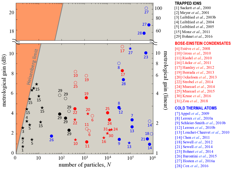
A variety of techniques have been used to generate entangled states useful for quantum metrology with atomic ensembles. The crucial ingredient is interaction between the particles, for instance atom-atom collisions in Bose-Einstein condensates, atom-light interactions in cold thermal ensembles (including experiments performed with warm vapors in glass cells), or combined electrostatic and ion-light interaction in ion chains. Figure 2 summarizes the experimental achievements (gain of phase sensitivity relative to the standard quantum limit) as a function of the number of particles. Stars in Fig. 2 show the measured phase-sensitivity gain obtained after a full interferometer sequence using entangled states as input to the atom interferometer. Filled circles report witnesses of metrologically useful entanglement (i.e., spin squeezing and Fisher information) measured on experimentally generated states, representing potential improvement in sensitivity. Open circles are inferred squeezing, being obtained after subtraction of detection noise. The Heisenberg limit has been reached with up to 10 trapped ions. Attaining this ultimate bound with a much larger number of particles is beyond current technology as it requires the creation and protection of large amounts of entanglement. Nevertheless, metrological gains up to 100 have been reported with large atomic ensembles Hosten et al. (2016a). A glance at Fig. 2 reveals how quantum metrology with atomic ensembles is a very active area of research in physics. Moreover, the reported results prove that the field is now mature enough to take the step from proofs-of-principle to technological applications.
I.4 Outline
This Review presents modern developments of phase-estimation techniques in atomic systems aided by quantum-mechanical entanglement, as well as fundamental studies of the associated entangled states. In Sec. II, we give a theoretical overview of quantum-enhanced metrology. We first discuss the concepts of spin squeezing and Fisher information considering spin-1/2 particles. We then illustrate different atomic systems where quantum-enhanced phase estimation—or, at least, the creation of useful entanglement for quantum metrology—has been demonstrated. Sections III and IV review the generation of entangled states in Bose-Einstein condensates. Section V describes the generation of entangled states of many atoms through the common coupling to an external light field. Section VI describes metrology with ensembles of trapped ions. Finally, Sec. VII gives an overview of the experimentally realized entanglement-enhanced interferometers and the realistic perspective to increase the sensitivity of state-of-the-art atomic clocks and magnetometers. This section also discusses the impact of noise in the different interferometric protocols.
II Fundamentals
In this Review we consider systems and operations involving particles and assume that all of their degrees of freedom are restricted to only two modes (single-particle states) that we identify as and . These can be two hyperfine states of an atom, as in a Ramsey interferometer Ramsey (1963), two energy levels of a trapping potential, or two spatially-separated arms, as in a Mach-Zehnder interferometer Zehnder (1891); Mach (1892), see Fig. 3. The interferometer operations are collective, acting on all particles in an identical way. The idealized formal description of these interferometer models is mathematically equivalent Wineland et al. (1994); Lee et al. (2002): as discussed in Sec. II.1, it corresponds to the rotation of a collective spin.

II.1 Collective spin systems
Single spin.
By identifying mode with spin-up and mode with spin-down, a (two-mode) atom can be described as an effective spin-1/2 particle: a qubit Nielsen and Chuang (2000); Peres (1995). Any pure state of a single qubit can be written as , with and the polar and azimuthal angle, respectively, in the Bloch sphere. Pure states satisfy , where is the Pauli vector and is the mean spin direction. Mixed qubit states can be expressed as , and have an additional degree of freedom given by the length of the spin vector , such that the effective state vector lies inside the Bloch sphere.
Many spins.
To describe an ensemble of distinguishable qubits, we can introduce the collective spin vector , where
| (1) |
and is the Pauli vector of the th particle. In particular, is half the difference in the populations of the two modes. The operators (1) satisfy the angular-momentum commutation relations
| (2) |
and have a linear degenerate spectrum spanning the -dimensional Hilbert space. The well-known set of states forms a basis, where and , and as well as Zare (1988).
Many spins in a symmetrized state.
The Hilbert space spanned by many-qubit states symmetric under particle exchange is that of total spin , which is the maximum allowed spin length for particles. It has dimension , linearly increasing with the number of qubits. Symmetric qubit states are naturally obtained for indistinguishable bosons and are described by the elegant formalism developed by Schwinger in the 1950s Biederharn and Louck (1981). Angular momentum operators are expressed in terms of bosonic creation, and , and annihilation, and , operators for the two modes and :
| (3) |
They satisfy the commutation relations (2) and commute with the total number of particles . The common eigenstates of and are called Dicke states Dicke (1954) or two-mode Fock states,
| (4) | |||||
where is the vacuum. They correspond to the symmetrized combinations of particles in mode and particles in mode , where . The eigenstates along an arbitrary spin direction can be obtained by a proper rotation of : and , for instance. Finally, it is useful to introduce raising and lowering operators, ( and ), transforming the Dicke states as .
Collective rotations.
Any unitary transformation of a single qubit is a rotation on the Bloch sphere, where and are the rotation axis and rotation angle, respectively. With qubits, each locally rotated about the same axis and angle , the transformation is , where is the generation of the collective rotation. This is the idealized model of most of the interferometric transformations discussed in this Review. In the collective-spin language, a balanced beam splitter is described by , and a relative phase shift by . Combining the three transformations, , the whole interferometer sequence (Mach-Zehnder or Ramsey), is equivalent to a collective rotation around the -axis on the generalized Bloch sphere of maximum radius Yurke et al. (1986), see Fig. 3(c).
II.2 Phase estimation
Broadly speaking, an interferometer is any apparatus that transforms a probe state depending on the value of an unknown phase shift , see Fig. 1. The parameter cannot be measured directly and its estimation proceeds from the results of measurements performed on identical copies of the output state . There are good and bad choices for a measurement observable. Good ones (that we will quantify and discuss in more details below) are those characterized by a statistical distribution of measurement results that is maximally sensitive to changes of . We indicate as the probability of a result222 In a simple scenario, is the eigenvalue of an observable. In a more general situation, the measurement is described by a positive-operator-values measure (POVM). A POVM is a set of Hermitian operators parametrized by Nielsen and Chuang (2000) that are positive, , to guarantee non-negative probabilities , and satisfy , to ensure normalization . given that the parameter has the value . The probability of observing the sequence of independent measurements is . An estimator is a generic function associating each set of measurement outcomes with an estimate of . Interference fringes of a Ramsey interferometer are a familiar example of such an estimation (they belong to a more general estimation technique known as the method of moments, discussed in II.2.6). Since the estimator is a function of random outcomes, it is itself a random variable. It is thus characterized by a -dependent statistical mean value and variance
| (5) |
the sum extending over all possible sequences of measurement results. Different estimators can yield very different results when applied to the same measured data. In the following, we will be interested in locally-unbiased estimators, i.e., those for which and , so that the statistical average yields the true parameter value.
II.2.1 Cramér-Rao bound and Fisher information
How precise can a statistical estimation be? Are there any fundamental limits? A first answer came in the 1940s with the works of Cramér (1946), Rao (1945), and Fréchet (1943), who independently found a lower bound to the variance (5) of any arbitrary estimator. The Cramér-Rao bound is one of the most important results in parameter-estimation theory. For an unbiased estimator and independent measurements, the Cramér-Rao bound reads
| (6) |
where
| (7) |
is the Fisher information Fisher (1922, 1925), the sum extending over all possible values of . The factor in Eq. (6) is the statistical improvement when performing independent measurements on identical copies of the probe state. The Cramér-Rao bound assumes mild differentiability properties of the likelihood function and thus holds under very general conditions,333The Cramér-Rao theorem follows from , that implies , and the Cauchy-Schwarz inequality . The equality is obtained if and only if with independent on . Equation (6) is recovered for unbiased estimators, i.e., , using the additivity of the Fisher information, . see for instance Kay (1993). No general unbiased estimator is known for small . In the central limit, , at least one efficient and unbiased estimator exists in general: the maximum of the likelihood, see Sec. II.2.5.
II.2.2 Lower bound to the Fisher information
A lower bound to the Fisher information can be obtained from the rate of change with of specific moments of the probability distribution Pezzè and Smerzi (2009):
| (8) |
where , and . The Fisher information is larger because it depends on the full probability distribution rather than some moments.
Lower bounds to the Fisher information can be also obtained from reduced probability distributions. These are useful, for instance, when estimating the phase shift encoded in a many-body distribution from the reduced one-body density, e.g., from the intensity of a spatial interference pattern Chwedeńczuk et al. (2012). One find
| (9) |
where is the Fisher information corresponding to the one-body density , and the coefficient further depends on the two-body density . Notice that in absence of correlations, namely .
II.2.3 Upper bound to the Fisher information: the quantum Fisher information
An upper bound to the Fisher information is obtained by maximizing Eq. (7) over all possible generalized measurements in quantum mechanics Braunstein and Caves (1994), , called the quantum Fisher information (see footnote 2 for the notion of generalized measurements and their connection to conditional probabilities). We have , and the corresponding bound on the phase sensitivity for unbiased estimators and independent measurements is
| (10) |
called the quantum Cramér-Rao bound Helstrom (1967). The quantum Fisher information and the quantum Cramér-Rao bound are fully determined by the interferometer output state . Hence they allow to calculate the optimal phase sensitivity of any given probe state and interferometer transformation Helstrom (1976); Holevo (1982), for recent reviews see Paris (2009); Giovannetti et al. (2011); Pezzè and Smerzi (2014). In general, the quantum Fisher information can be expressed as the variance of a -dependent Hermitian operator called the symmetric logarithmic derivative and defined as the solution of Helstrom (1967). A general expression of the quantum Fisher information can be found in terms of the spectral decomposition of the output state where both the eigenvalues and the associated eigenvectors depend on Braunstein and Caves (1994):
| (11) |
showing that depends solely on and its first derivative . We can decompose this equation as
| (12) |
The first term quantifies the information about encoded in and corresponds to the Fisher information obtained when projecting over the eigenstates of . The second term accounts for change of eigenstates with (we indicate ). For pure states, , the first term in Eq. (12) vanishes, while the second term simplifies dramatically to .
For unitary transformations generated by some Hermitian operator , we have , and Eq. (12) becomes444We use the notation to indicate the quantum Fisher information for a generic transformation of the probe state, and for unitary transformations. Braunstein and Caves (1994); Braunstein et al. (1996)
| (13) |
For pure states , Eq. (13) reduces to . For mixed states, . It is worth recalling here that , where and are the maximum and minimum eigenvalues of with eigenvectors and , respectively. This bound is saturated by the states , with arbitrary real , which are optimal input states for noiseless quantum metrology. In presence of noise, the search for optimal quantum states is less straightforward, as discussed in Sec. VII.1.
Convexity and additivity.
The quantum Fisher information is convex in the state:
| (14) |
with . This expresses the fact that mixing quantum states cannot increase the achievable estimation sensitivity. The inequality (14) can be proved using the fact that the Fisher information is convex in the state Cohen (1968); Pezzè and Smerzi (2014).
Optimal measurements.
The equality can always be achieved by optimizing over all possible measurements. A possible optimal choice of measurement for both pure and mixed states is given by the set of projectors onto the eigenstates of Braunstein and Caves (1994). This set of observables is necessary and sufficient for the saturation of the quantum Fisher information whenever is invertible, and only sufficient otherwise. In particular, for pure states and unitary transformations, the quantum Cramér-Rao bound can be saturated, in the limit , by a dichotomic measurement given by the projection onto the probe state itself, , and onto the orthogonal subspace, Pezzè and Smerzi (2014). It should be noted that the symmetric logarithmic derivative, and thus also the optimal measurement, generally depends on , even for unitary transformations. Nevertheless, without any prior knowledge of , the quantum Cramér-Rao bound can be saturated in the asymptotic limit of large using adaptive schemes Hayashi (2005); Fujiwara (2006).
Optimal rotation direction.
Given a probe state, and considering a unitary transformation generated by , it is possible to optimize the rotation direction in order to maximize the quantum Fisher information Hyllus et al. (2010). This optimum is given by the maximum eigenvalue of the matrix
| (16) |
with , and the optimal direction by the corresponding eigenvector. For pure states, .

II.2.4 Phase sensitivity and statistical distance
Parameter estimation is naturally related to the problem of distinguishing neighboring quantum states along a path in the parameter space Wootters (1981); Braunstein and Caves (1994). Heuristically, the phase sensitivity of an interferometer can be understood as the smallest phase shift for which the output state of the interferometer can be distinguished from the input . We introduce a statistical distance between probability distributions,
| (17) |
called the Hellinger distance, where is the statistical fidelity, or overlap, between probability distributions, also known as Bhattacharyya coefficient Bhattacharyya (1943). is non-negative, , and its Taylor expansion reads
| (18) |
This equation reveals that the Fisher information is the square of a statistical speed, . It measures the rate at which a probability distribution varies when tuning the phase parameter . Equation (18) has been used to extract the Fisher information experimentally Strobel et al. (2014), see Sec. III.3. As Eq. (17) depends on the specific measurement, it is possible to associate different statistical distances to the same quantum states. This justifies the introduction of a distance between quantum states by maximizing over all possible generalized measurements (i.e., over all POVM sets, see footnote 2), Fuchs and Caves (1995), called the Bures distance Bures (1969). Hübner (1992) showed that
| (19) |
where is the transition probability Uhlmann (1976) or the quantum fidelity between states Jozsa (1994), see Bengtsson and Zyczkowski (2006); Spehner (2014) for reviews. Uhlmann’s theorem Uhlmann (1976) states that , where the maximization runs over all purifications of and of Nielsen and Chuang (2000). In particular, for pure states. A Taylor expansion of Eq. (19) for small gives
| (20) |
The quantum Fisher information is thus the square of a quantum statistical speed, , maximized over all possible generalized measurements. The quantum Fisher information has also been related to the dynamical susceptibility Hauke et al. (2016), while lower bounds have been derived by Apellaniz et al. (2017) and Frérot and Roscilde (2016).
II.2.5 The maximum likelihood estimator
The maximum likelihood estimator is the phase value that maximizes the likelihood of the observed measurement sequence , see Fig. 4(a): . The key role played by in parameter estimation is due to its asymptotic properties for independent measurements. For sufficiently large , the distribution of the maximum likelihood estimator tends to a Gaussian centered at the true value and of variance equal to the inverse Fisher information Lehmann and Casella (2003): . Therefore, the maximum likelihood estimator is asymptotically unbiased and its variance saturates the Cramér-Rao bound: . In the central limit, any estimator is as good as—or worse than—the maximum likelihood estimate.
II.2.6 Method of moments
The method of moments exploits the variation of collective properties of the probability distribution—such as the mean value and variance —with the phase shift . Let us take the average of measurements results . The estimator is the value for which is equal to , see Fig. 4(b). Applying this method requires to be a monotonous function of the parameter , at least in a local region of parameter values determined from prior knowledge. The sensitivity of this estimator can be calculated by error propagation,555A Taylor expansion of around the true value gives . We obtain Eq. (21) by identifying (valid for ) and . giving
| (21) |
As expected on general grounds and proved by Eq. (8), the method of moments is not optimal in general, , with no guarantee of saturation even in the central limit. The equality is obtained when the probability distribution is Gaussian, , and , such that the changes of the complete probability distribution are fully captured by the shift of its mean value Pezzè and Smerzi (2014). Nevertheless, due to its simplicity, Eq. (21) is largely used in the literature to calculate the phase sensitivity of an interferometer for various input states and measurement observables Wineland et al. (1994); Dowling (1998); Yurke et al. (1986). For instance, in the case of unitary rotations generated by (as in Ramsey and Mach-Zehnder interferometers) and taking as measurement observable, Eq. (21) in the limit can be rewritten as
| (22) |
This equation is useful to introduce the concept of metrological spin-squeezing, see Sec. II.3.5. We recall that Eqs. (21) and (22) are valid for a sufficiently large number of measurements.
Finally, there are many examples in the literature where a small is obtained for phase values where , while the ratio remains finite Yurke et al. (1986); Kim et al. (1998). These “sweet spots” are very sensitive to technical noise: an infinitesimal amount of noise may prevent to vanish, while leaving unchanged , such that diverges Lücke et al. (2011).
II.2.7 Bayesian estimation
The cornerstone of Bayesian inference is Bayes’ theorem. Let us consider two random variables and . Their joint probability density can be expressed as in terms of the conditional probability and the marginal probability distribution . Bayes’ theorem
| (23) |
follows from the symmetry of the joint probability .
In the Bayesian subjective interpretation of probabilities, and are both considered as random variables with as the posterior probability distribution given the measurement results . is the prior probability distribution that quantifies our (subjective) ignorance of the true value of the interferometric phase, i.e., before any measurements were done. One often has no prior knowledge on the phase (maximum ignorance), which is expressed by a flat prior distribution . Bayes’ theorem allows to update our knowledge about the interferometric phase by including measurement results, since can be calculated directly (see the introduction of Sec. II.2) and is determined by the normalization . Bayesian probabilities express our (lack of) knowledge of the interferometric phase as a probability distribution . This is radically different from the standard frequentist view where the probability is defined as the infinite-sample limit of the outcome frequency of an observed event. Having the posterior distribution , we can consider any phase as the estimate. In practice, it is convenient to choose the weighted averaged , or the phase corresponding to the maximum of the probability , since the corresponding mean square fluctuations saturate the Cramér-Rao bound (see below). We can further calculate the probability that the chosen estimate falls into a certain interval by integrating . To take into account the periodicity of the probability, quantities like can be calculated. Remarkably, Bayesian estimation is asymptotically consistent: as the number of measurements increases, the posterior probability distribution assigns more weight in the vicinity of the true value. The Laplace-Bernstein-von Mises theorem Lehmann and Casella (2003); Pezzè and Smerzi (2014); Gill (2008) demonstrates that, under quite general conditions, , to leading order in , for . In this limit, the posterior probability becomes normally distributed, centered at the true value of the parameter, and with a variance inversely proportional to the Fisher information. See Van Trees and Bell (2007) for a review of bounds in Bayesian phase estimation.
II.3 Entanglement and phase sensitivity
In this section we show how entanglement can offer a precision enhancement in quantum metrology. We start with the formal definition of multiparticle entanglement and then clarify, via the Fisher information introduced in the previous section, the notion of useful entanglement for quantum metrology.
II.3.1 Multiparticle entanglement
Let us consider a system of particles (labeled as ), each particle realizing a qubit. A pure quantum state is separable in the particles if it can be written as a product
| (24) |
where is the state of the th qubit. A mixed state is separable if it can be written as a mixture of product states Werner (1989),
| (25) |
with and . States that are not separable are called entangled Horodecki et al. (2009); Gühne and Tóth (2009). In the case of particles, any quantum state is either separable or entangled. For , we need further classifications Dür et al. (2000). Multiparticle entanglement is quantified by the number of particles in the largest non-separable subset. In analogy with Eq. (24), a pure state of particles is -separable (also indicated as -producible in the literature) if it can be written as
| (26) |
where is the state of particles and . A mixed state is -separable if it can be written as a mixture of -separable pure states Gühne et al. (2005)
| (27) |
A state that is -separable but not -separable is called -particle entangled: it contains at least one state of particles that does not factorize. Using another terminology Sørensen and Mølmer (2001), it has an entanglement depth larger than . In maximally entangled states () each particle is entangled with all the others. Finally, note that -separable states form a convex set containing the set of -separable states with Gühne and Tóth (2009).
II.3.2 Sensitivity bound for separable states: the standard quantum limit
The quantum Fisher information of any separable state of qubits is upper-bounded Pezzè and Smerzi (2009):
| (28) |
This inequality follows from the convexity and additivity of the quantum Fisher information and uses Pezzè and Smerzi (2014). As a consequence of Eqs. (10) and (28), the maximum phase sensitivity achievable with separable states is Giovannetti et al. (2006)
| (29) |
generally indicated as the shot-noise or standard quantum limit. This bound is independent of the specific measurement and estimator, and refers to unitary collective transformations that are local in the particles. In Eq. (29) and play the same role: repeating the phase estimation times with one particle has the same sensitivity bound as repeating the phase estimation one time with particles in a separable state.
II.3.3 Coherent spin states
The notion of coherent spin states was introduced by Arecchi et al. (1972); Radcliffe (1971) as a generalization of the field coherent states first discussed by Glauber (1963), see Zhang et al. (1990) for a review. Coherent spin states are constructed as the product of qubits (spins-1/2) in pure states all pointing along the same mean-spin direction :
| (30) |
Equation (30) is the eigenstate of with the maximum eigenvalue of . The coherent spin state is a product state and no quantum entanglement is present between the particles. can also be written as a binomial sum of Dicke states with Arecchi et al. (1972). When measuring the spin component of along any direction orthogonal to , each individual atom is projected with equal probability into the up and down eigenstates along this axis, with eigenvalues , respectively: we thus have , and Itano et al. (1993); Yurke et al. (1986).
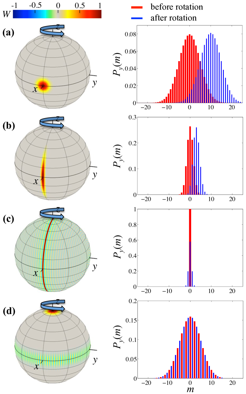
Coherent spin states are optimal separable states for metrology. They saturate the equality sign in Eq. (28) and thus reach the standard quantum limit. Let us consider the rotation of around a direction perpendicular to the mean spin direction (here , and are mutually orthogonal). This rotation displaces the coherent spin state on the surface of the Bloch sphere, see Fig. 5(a). The initial and final states become distinguishable after rotating by an angle heuristically giving the phase sensitivity of the state. This rotation angle can be obtained from a geometric reasoning Yurke et al. (1986): we have , giving for . More rigorously, the squared Bures distance, Eq. (19), between and the rotated is
| (31) |
that is for small values of . According to Eq. (13) we obtain a quantum Fisher information . With the method of moments, Eq. (22), we find a phase sensitivity Itano et al. (1993); Yurke et al. (1986): while reaches its maximum value, it is the quantum projection noise of uncorrelated atoms, , that limits the achievable sensitivity Itano et al. (1993); Wineland et al. (1992, 1994). For any rotation around an axis orthogonal to the mean spin direction, coherent spin states thus satisfy .
II.3.4 Useful entanglement for quantum metrology
The violation of Eq. (28), i.e.,
| (32) |
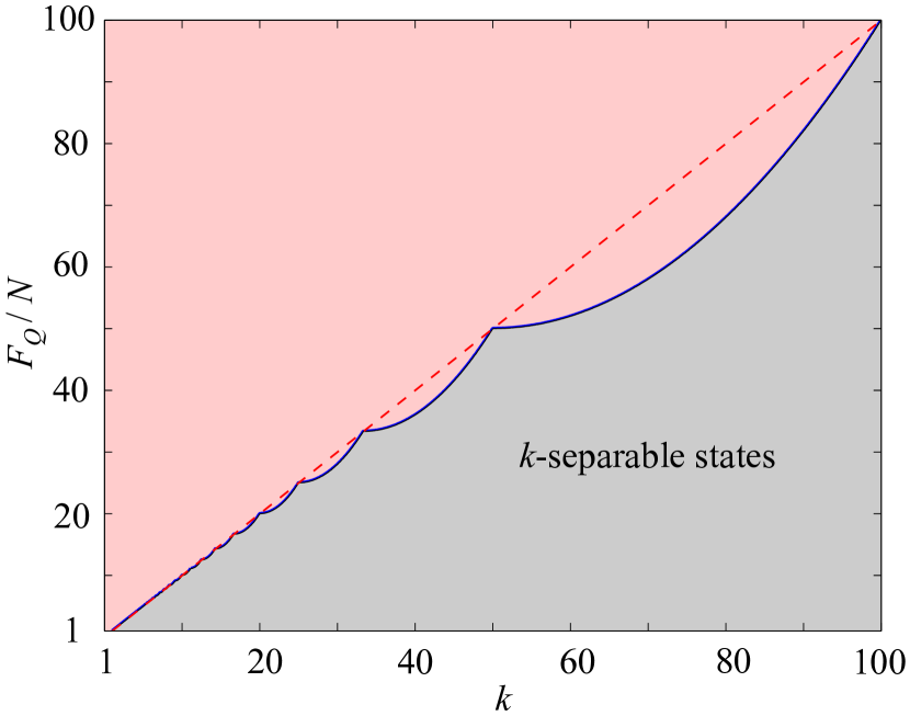
is a sufficient condition for particle-entanglement in the state . To be more precise, the inequality (32) is the condition of useful entanglement for quantum metrology: it is a necessary and sufficient condition for a quantum state to be useful in the estimation of a phase shift —with an interferometer implementing the transformation —with a sensitivity overcoming the standard quantum limit Pezzè and Smerzi (2009). Not all entangled states are useful for quantum metrology. Yet, useless entangled states for quantum metrology might be useful for other quantum technologies. It should also be noted that not all useful entangled states for quantum metrology are equally useful: large quantum Fisher information requires large entanglement depth. For states of type (27), we have Hyllus et al. (2012a); Tóth (2012)
| (33) |
where is the integer part of , and (note that when is divisible by ). If the bound (33) is surpassed, then the probe state contains metrologically useful -particle entanglement: when used as input state of the interferometer defined by the transformation , this state enables a phase sensitivity better than any -separable state. The bound (33) increases monotonically with (see Fig. 6), in particular . The maximum value of the quantum Fisher information is obtained for genuine -particle entangled states, , giving Pezzè and Smerzi (2009)
| (34) |
Equation (34) defines the ultimate Heisenberg limit666The name “Heisenberg limit” was first introduced in Holland and Burnett (1993) referring to the heuristic number-phase Heisenberg uncertainty relation . We refer to the Heisenberg scaling of phase sensitivity when . 777It is possible to maximize the phase sensitivity by optimizing the number of particles entering into the interferometer multiplied by the times that the measurement is performed Lane et al. (1993); Pezzé (2013); Braunstein et al. (1992). This provides a definition of Heisenberg limit , where , and is the optimal number of measurements that maximize the phase sensitivity for a fixed number of particles . Since may depend on , there might be, in principle, states having a Fisher information larger than but a phase variance above the standard quantum limit . of phase sensitivity Giovannetti et al. (2006),
| (35) |
The difference between Eq. (29) and Eq. (35) is a faster scaling of the phase sensitivity with the number of particles, which cannot be obtained by exploiting classical correlations among the qubits. Still the standard quantum limit can be surpassed using separable states at the expense of other resources Giovannetti et al. (2006) such as, for instance, exploiting a multiround protocol Higgins et al. (2007).
We note that the quantum Fisher information is bounded by , where is the spin length. This shows that the most sensitive states lie in a subspace with maximum spin , namely those symmetric under particle exchange (see Sec. II.1).
Equations (29) and (35) can be generalized to transformations , where is an arbitrary local Hamiltonian for the th particles (that can be a generic qudit). Taking for all particles, we have , and Giovannetti et al. (2006), where , and and are the maximum and minimum eigenvalues of , respectively.
We finally note that not all -particle entangled states reach the Heisenberg limit, as exemplified by the generalized state , which corresponds to a Dicke state with one excitation. While the state is -particle entangled Dür et al. (2000), its quantum Fisher information only amounts to .
II.3.5 Metrological spin squeezing
Spin-squeezed states are a class of states having squeezed spin variance along a certain direction, at the cost of anti-squeezed variance along an orthogonal direction. Spin squeezing is one of the most successful approaches to witness large-scale quantum entanglement beating the standard quantum limit in interferometry.
Let us consider the unitary rotation of a state on the Bloch sphere around an axis perpendicular to the mean spin direction , see Fig. 5(b), and calculate the phase sensitivity according to the error propagation formula, Eq. (22). We can write , 888In the literature, it is possible to find different notations for the metrological spin-squeezing parameter (e.g., and are also commonly used). Here we follow the notation first introduced by Wineland et al. (1994) and used in a previous review Ma et al. (2011). In particular, in this review refers to the Kitagawa and Ueda (1993) spin-squeezing parameter, see Eq. 45. where
| (36) |
and is orthogonal to both and . is the spin-squeezing parameter introduced by Wineland et al. (1992, 1994). If holds, the state is said to be (metrologically) spin squeezed along the -axis Wineland et al. (1992, 1994) and it can be used to overcome the standard quantum limit (i.e., reaching ). This requires states having spin fluctuations orthogonal to the rotation axis smaller than the projection noise of uncorrelated atoms, i.e., , and sufficiently large spin length .
He et al. (2012) have generalized this criterion to systems of fluctuating numbers of particles by introducing scaled spin operators in terms of the Moore-Penrose pseudoinverse of the particle number operator.
Optimal spin-squeezed states.
Optimal spin-squeezed states are searched among the so-called minimum uncertainty states Aragone et al. (1974); Rashid (1978); Wòdkiewicz and Eberly (1985). These states saturate the Heisenberg uncertainty relation
| (37) |
since . We thus have and a lower bound to is obtained by maximizing , giving Hillery and Mlodinow (1993); Agarwal and Puri (1994)
| (38) |
This bound can be saturated by the state in the limit Brif and Mann (1996), where are Dicke states defined in Sec. II.1. Notice that spin-squeezed states can achieve a Heisenberg scaling of phase sensitivity, , but not the Heisenberg limit (35) for . Optimal spin-squeezed states for even values of and fixed values of are given by the ground state of the Hamiltonian , where is a Lagrange multiplier Sørensen and Mølmer (2001).

Spin squeezing and bosonic quadrature squeezing.
In the case of probe states having and a strong population imbalance between the two modes, spin squeezing can be well approximated by single-mode quadrature-squeezing. Let be the highly-populated mode (continuous-variable limit, ) and perform the Holstein-Primakoff transformation Wang and Sanders (2003a); Madsen and Mølmer (2004); Duan et al. (2002) , , and , formally equivalent to the mean-field replacement . Within this approximation, the rescaled spin operators and map onto the position and momentum quadrature operators Scully and Zubairy (1997), respectively. We thus find
| (39) |
where and . Equation (39) shows the equivalence between the metrological spin-squeezing parameter and the quadrature variance, within the approximations. In particular, the rotation maps onto a displacement of the state along the direction in the quadrature plane by an amount , described by , see Fig. 7. When squeezing the quadrature variance below the vacuum noise limit, i.e., , it is possible to overcome the standard quantum limit of phase sensitivity, i.e., . The sensitivity of interferometers using a probe state with all atoms in a single mode can be increased by feeding the other mode with a quadrature-squeezed state, as first proposed by Caves (1981) for an optical interferometer.
Spin squeezing, entanglement and Fisher information.
Spin squeezing is a sufficient condition for useful particle entanglement in metrology Sørensen et al. (2001). Furthermore, Sørensen and Mølmer (2001) showed that the degree of spin squeezing is related to metrologically useful -particle entanglement: for a given spin length, smaller and smaller values of can only be obtained by increasing the entanglement depth, see Fig. 8. The quantum Fisher information detects entanglement in a larger number of states than those recognized by metrological spin squeezing Pezzè and Smerzi (2009):
| (40) |
This inequality, which follows from Eq. (8), shows that if a state is spin squeezed, , it also satisfies the condition of metrologically useful entanglement, . The contrary is not true: there are states that are not spin squeezed and yet entangled and useful for quantum metrology. The Dicke and NOON states, discussed below, are important examples.
II.3.6 Dicke states
Dicke states, Eq. (4), have a precise relative number of particles between the two modes and a completely undefined phase. They are not spin squeezed Wang and Mølmer (2002). A direct calculation of the quantum Fisher information gives
| (41) |
for any rotation direction orthogonal to the axis. Dicke states with are coherent spin states; those with are metrologically usefully entangled. From the perspective of quantum metrology, the most interesting Dicke state is the twin-Fock state Holland and Burnett (1993); Sanders and Milburn (1995), , corresponding to particles in each mode. It can be visualized as a ring on the equator of the Bloch sphere, see Fig. 5(c). A rotation around any axis in the - plane converts the well-defined number difference into a well defined relative phase between the two modes. It should be noted that the twin-Fock state has zero mean spin length. Therefore, the metrologically useful entanglement of the twin-Fock state cannot be exploited when measuring the relative number of particles. A possible phase-sensitive signal is the variance of the relative population Kim et al. (1998), see Sec. IV.2.2. The phase sensitivity calculated via the method of moments strongly depends on : for and , we have , which is a factor two above the Heisenberg limit at and remains below the standard quantum limit for . Similar results can be obtained with error propagation when estimating the phase shift from the measurement of the parity operator Campos et al. (2003); Gerry et al. (2004). Parity measures the difference in populations between even and odd eigenstates of and can be difficult to implement for large spins. A -independent phase sensitivity can be reached when measuring the number of particles at the output ports of the interferometer and using a maximum likelihood estimator or a Bayesian method Krischek et al. (2011); Holland and Burnett (1993); Pezzè and Smerzi (2006).
Squeezing the number of particles at both inputs of the interferometer is not necessary to overcome the standard quantum limit Pezzè and Smerzi (2013). Let us consider a probe state , where is an arbitrary state in mode with mean particle number and is a Fock state of particles in mode . We find
| (42) |
Heisenberg scaling is achieved when , without any assumptions on . In particular, existing interferometers that operate with uncorrelated atoms can be improved by simply replacing the vacuum state in one of the two input ports by a Fock state.
II.3.7 NOON states
The Heisenberg limit can be saturated by the state
| (43) |
given by a coherent superposition of all particles in mode and all particles in mode , where is an arbitrary phase. This state is called NOON state Lee et al. (2002) when considering indistinguishable bosonic particles. When considering distinguishable particles, as ions in a Paul trap for instance, see Sec. VI, the state (43) is generally called a “Schrödinger cat” Bollinger et al. (1996); Leibfried et al. (2005) or Greenberger-Horne-Zeilinger state Monz et al. (2011), originally introduced in Greenberger et al. (1990) for three particles. A look at the Wigner distribution of the NOON state, see Fig. 5(d,left), reveals substructures of angular size given by spherical harmonic contributions with the maximum allowed value Schmied and Treutlein (2011). Rotating the NOON state around the -axis, the initial and final states becomes distinguishable after a rotation angle . The squared Bures distance between the probe and the rotated state is
| (44) |
which oscillates in phase time faster than the corresponding overlap for a coherent spin state, Eq. (31), and is for small Pezzè and Smerzi (2007). Note that the relative spin probability distribution of the NOON state, , see Fig. 5(d,right), shows a comb-like structure as a function of . These substructure change quickly with : for only even values of are populated, for only odd values of are populated, with . According to Eq. (13), we obtain , and thus for the NOON state. It is possible to reach this sensitivity via the method of moments by measuring the parity of the relative number of particles among the two modes Bollinger et al. (1996), see also Sec. VI.2.2.
II.3.8 Further notions of spin squeezing and their relation to entanglement
When it is not possible to address individual qubits, or in presence of low counting statistics, entanglement criteria based on the measurement of collective properties—as the condition introduced in Sec. II.3.5—are experimentally important. Moreover, states of a large number of particles cannot be characterized via full state tomography: the reconstruction of the full density matrix is hindered and finally prevented by the exponential increase in the required number of measurements. In the literature, different definitions of spin squeezing for collective angular momentum operators can be found Ma et al. (2011); Tóth and Apellaniz (2014). In the following we review the ones most relevant for the present context.

Squeezing parameter of Kitagawa and Ueda.
A spin-1/2 particle is characterized by isotropic spin fluctuations, equal to 1/4, along any direction orthogonal to the mean spin direction . By adding uncorrelated spins all pointing along (as in a coherent spin state), we have , where is an arbitrary direction orthogonal to . Quantum correlations between spins may result in reduced fluctuations in one direction, , at the expense of enhanced fluctuations along the other direction orthogonal to . This suggests the introduction of the spin-squeezing parameter Kitagawa and Ueda (1993)
| (45) |
being the spin-squeezing condition. Equation (45) is related to metrological spin squeezing via the relation . Since , we obtain
| (46) |
In other words, metrological spin squeezing, , implies spin squeezing according to the definition of Kitagawa and Ueda. The converse is not true: there is no direct relation between and the improvement of metrological sensitivity, as illustrated in Fig. 8. It is worth noting that the minimum in Eq. (45) is given by the smallest eigenvalue of the covariance matrix , where are two mutually orthogonal directions in the plane perpendicular to and . Taking, without loss of generality, , we have Wang and Sanders (2003b)
| (47) |
Entanglement witnessed by mean values and variances of spin operators.
For separable states (25), the inequalities
| (48a) | |||
| (48b) | |||
| (48c) | |||
| (48d) | |||
are all fulfilled, where , and are three mutually orthogonal directions. The violation of at least one of the above inequalities signals that the state is entangled. Equation (48a) is equivalent to , see Sec. II.3.5, and was introduced by Sørensen et al. (2001). The inequalities (48b)-(48d) have been introduced by Tóth et al. (2007, 2009). A violation of the condition (48b) can be used to detect entanglement in singlet states Tóth and Mitchell (2010); Behbood et al. (2014). The third condition, Eq. (48c), can be rewritten as , where
| (49) |
In particular, the condition can be used to detect entanglement close to Dicke states Tóth et al. (2007), see also Raghavan et al. (2001). The detection of multiparticle entanglement close to Dicke states for spin-1/2 particles has been studied by Duan (2011); Lücke et al. (2014) and for spin- particles with by Vitagliano et al. (2017). The inequalities (48b)-(48d) and the further inequality , which is valid for all quantum states (not only for separable states), form a system of conditions that defines a polytope in the three dimensional space with coordinates , , and Tóth et al. (2007, 2009). The polytope encloses all separable states. It has been demonstrated that Eqs. (48) form a complete set Tóth et al. (2007, 2009), meaning that it is not possible to add new entanglement conditions based on mean values and variances of spin moments that detect more entangled states. The inequalities (48) have been generalized to arbitrary spin systems Vitagliano et al. (2011, 2014) and to systems of fluctuating numbers of particles Hyllus et al. (2012b). Furthermore, Korbicz et al. (2005, 2006) have shown that, if the inequality
| (50) |
holds, then the state possesses pairwise entanglement, i.e., entanglement in the two-qubit reduced density matrix obtained by tracing the qubit state over all particles except the th and th.
Spin squeezing and entanglement of symmetric states.
We emphasize that none of the entanglement witnesses above require any assumptions on the symmetry of the state. For states that are symmetric under particle exchange, we have . In this case, Eq. (50) can be rewritten as
| (51) |
where is called the number-squeezing parameter. The inequality (51) is necessary and sufficient for pairwise entanglement Korbicz et al. (2005, 2006). It should be noted that if holds, then the inequality (51) is satisfied as well (taking and ). Hence, symmetric spin-squeezed states possess two-qubit entanglement. The converse is not true: since in Eq. (51) is not necessarily orthogonal to the mean spin direction , number squeezing () does not imply spin squeezing ().
The relationship between Kitagawa-Ueda spin squeezing and pairwise entanglement has also been studied by Ulam-Orgikh and Kitagawa (2001); Wang and Sanders (2003b). For an arbitrary symmetric state of qubits, the spin-squeezing parameter (45) can be written in terms of the two-spin correlation function Ulam-Orgikh and Kitagawa (2001)
| (52) |
This equation shows that spin squeezing is equivalent to negative pairwise spin-spin correlations that, in turn, are sufficient for pairwise entanglement.999The two-qubit reduced density matrix of a separable symmetric state of qubits has positive pairwise correlations: for any Wang and Sanders (2003b). Furthermore, for symmetric pure states of two qubits, there is a direct correspondence between and the concurrence Ulam-Orgikh and Kitagawa (2001); Wang and Sanders (2003b): . We recall that is a necessary and sufficient condition of—and quantifies—entanglement of a pair of qubits Hill and Wootters (1997); Wootters (1998). Symmetric pure states of two qubits are entangled if and only if they satisfy Ulam-Orgikh and Kitagawa (2001). For symmetric states of qubits that fulfill and other conditions,101010Equation (53) has been derived in Wang and Sanders (2003b) for symmetric states having and , , where and are vectors orthogonal to the mean spin direction . the equality
| (53) |
holds Wang and Sanders (2003b), where is calculated from the two-particles reduced density matrix. Equantion (53) tells us that implies and thus pairwise entanglement. When , Eq. (53) breaks down and we cannot draw any conclusion about pairwise entanglement: for example, Dicke states can be pairwise entangled even though they are not spin squeezed Wang and Mølmer (2002).
Planar spin-squeezed states.
While many useful spin-squeezed states have reduced quantum fluctuations along a single spin direction (with a corresponding increase in fluctuations along a perpendicular direction), the spin commutation relations make it possible to reduce the fluctuations along two orthogonal spin directions simultaneously while increasing those along a third direction. Specifically, an initially coherent state along the direction can be squeezed in the perpendicular plane such that simultaneously and Puentes et al. (2013), which does not violate Heisenberg’s uncertainty relation, Eq. (37), if is reduced at the same time. In general, such planar spin-squeezed states reduce the variance sum below the coherent-state value of , ultimately limited by He et al. (2011a)
| (54) |
Planar spin-squeezed states are useful for interferometric phase measurements where the phase fluctuations and the number fluctuations are squeezed simultaneously (see Sec. V.1.1), while the spin length fluctuates significantly. Note that not all planar spin-squeezed states are entangled He et al. (2012); Puentes et al. (2013); Vitagliano et al. (2018); see Eqs. (48b) and (48d) for relevant entanglement criteria.
II.3.9 Einstein-Podolsky-Rosen entanglement and Bell correlations
Continuous variable and Einstein-Podolsky-Rosen entanglement
Let us consider two bosonic modes, and , and introduce the corresponding annihilation and creation operators. Mode-separable quantum states are defined as , where , , and is the state of the mode. Mode entanglement, i.e., , can be revealed by correlations between bosonic position and momentum quadratures Reid et al. (2009). Mode-separable states fulfill Duan et al. (2000a); Simon (2000)
| (55) |
where and are variances. A violation of this condition detects entanglement between the modes. It is also a necessary and sufficient condition for mode entanglement in Gaussian states Duan et al. (2000a); Simon (2000), see also Giovannetti et al. (2003); Walborn et al. (2009); Shchukin and Vogel (2005); Gessner et al. (2016, 2017) for further (and sharper) conditions. Mode entanglement finds several applications in quantum technologies Braunstein and van Loock (2005).
Correlations between quadrature variances are at the heart of the Einstein-Podolsky-Rosen (EPR) paradox Einstein et al. (1935). When the quadratures and are measured in independent realizations of the same state, the correlations allow for a prediction of and with inferred variances violating the Heisenberg uncertainty relation , known as EPR criterion Reid (1989); Reid et al. (2009). This extends the original EPR discussion that was limited to perfect quadrature correlations. Non-steerable states, including separable states, fulfill Reid (1989)
| (56) |
The violation of this condition witnesses a strong form of entanglement (“EPR entanglement”) necessary to fulfill the EPR criterion. With atoms, continuous-variable entanglement has been first proved with room-temperature vapor cells Julsgaard et al. (2001). With spinor Bose-Einstein condensates, mode entanglement Gross et al. (2011) and EPR entanglement Peise et al. (2015a) have been demonstrated, see Sec. IV.3.
Bell correlations.
The strongest form of correlations between particles are those that violate a Bell inequality Bell (1964). The existence of Bell correlations has profound implications for the foundations of physics and underpins quantum technologies such as quantum key distribution and certified randomness generation Brunner et al. (2014). Bell correlations have been observed in systems of at most a few (usually two) particles Freedman and Clauser (1972); Zhao et al. (2003); Eibl et al. (2003); Hofmann et al. (2012); Lanyon et al. (2014); Hensen et al. (2015); Aspect et al. (1982); Giustina et al. (2015); Shalm et al. (2015); Rosenfeld et al. (2017); Matsukevich et al. (2008), but their role in many-body systems is largely unexplored Tura et al. (2014).
Entanglement is necessary but not sufficient for Bell correlations Werner (1989); Brunner et al. (2014). Therefore, entanglement criteria as those discussed above, cannot be used to determine whether a system could violate a Bell inequality. In Schmied et al. (2016) a criterion in the spirit of a spin-squeezing parameter is derived to determine whether Bell correlations are present in an -particle quantum system. For any two axes and , the inequality
| (57) |
is satisfied for all states that are not Bell correlated. States that satisfy can violate the many-particle Bell inequality of Tura et al. (2014), which is a statement about the strength of two-body correlations, but does not imply the violation of a two-particle Bell inequality for every pair of particles. By optimizing Eq. (57) over the angle between the two axes, a criterion follows that facilitates comparison with well-known spin-squeezing criteria: for any two axes and perpendicular to each other,
| (58) |
is satisfied for all states that are not Bell correlated. A similar criterion that is violated more easily was derived by Wagner et al. (2017),
| (59) |
Detecting Bell correlations by violating inequality (57), (58), or (59) requires only collective manipulations and measurements on the entire -particle system. While this does not provide a loophole-free and device-independent Bell test, it is a powerful tool for characterizing correlations in many-body systems state-independently. Bell correlations according to Eqs. (57), (58), and (59) have been observed with Bose-Einstein condensates, see Sec. III.2.3.
II.4 Tomography of spin states
II.4.1 Spin-noise tomography
Spin-noise tomography is a widely-used technique to gain information about spin-squeezed states, whose main characteristics are captured by their second spin moments along the squeezing and anti-squeezing directions. For this tomography, the state is rotated by an angle using resonant Rabi rotations, followed by projective spin measurements along the -axis: defined in Eqs. (3) is measured by counting the numbers of particles in the two modes, see Sec. II.5. The th moment of these spin projections can be fit to a linear combination of and with , which allows interpolating these projective measurements to arbitrary angles . Also, technical noise sources can be characterized and their influence subtracted from the resulting moments; any spin squeezing concluded from these inferred moments will be called inferred spin squeezing. Since this method estimates spin projection moments separately, they do not necessarily fulfill all consistency criteria imposed by the positive-semi-definiteness of the density operator Schmied (2016). In practical situations concerning spin-squeezed states, however, this restriction is often irrelevant. The information captured from low-order spin moments through spin-noise tomography may be insufficient to characterize and visualize general spin states. Different techniques have been developed for full state tomography Blume-Kohout (2010); Paris and Řeháček (2004); Schmied and Treutlein (2011), estimating all spin moments up to order .
II.4.2 Visualizing spin states
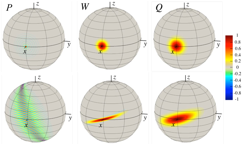
State representations on the Bloch sphere are very useful to gain an intuition about the properties of quantum states. In the following we consider symmetric states of spin-1/2 particles (see Sec. II.1). There are various representations in the form of pseudo-probability densities Schleich (2001). These are based on the decomposition of a general density operator into the ortho-normalized spherical tensor (or multipole) operators defined in terms of Clebsch-Gordan coefficients, with Arecchi et al. (1972); Agarwal (1981); Dowling et al. (1994); Schmied and Treutlein (2011). This decomposition has properties similar to the Fourier transform in Euclidean space: it separates low-frequency components (small ) from high-frequency components (large ), which are affected very differently by experimental noise. Further, it allows us to define the family of spherical functions Agarwal (1981)
| (60) |
in terms of spherical harmonics . All of these functions are linear in the density operator. The following representations (corresponding to different choices for the coefficients ) are often used, with examples given in Table 1 and Fig. 9.
| exact | ||
|---|---|---|
Wigner distribution.
The Wigner quasi-probability distribution Wigner (1932) corresponds to the case in Eq. (60). It is found by replacing the spherical tensor operators in the decomposition of by spherical harmonics of the same order, which obey the same ortho-normalization. Because of this close similarity, the Wigner quasi-probability distribution is equivalent to the density operator. is not a true probability density, as it can take negative values Leibfried et al. (1996); Lvovsky et al. (2001); McConnell et al. (2015). For continuous variables, this is often understood as a sign of nonclassical behavior. Note however that in the present finite-dimensional space, even the Wigner distribution of a coherent spin state has negative parts of amplitude , exponentially decreasing with the number of particles.
Husimi-Kano representation.
The Husimi-Kano Q representation Husimi (1940); Haas et al. (2014); Barontini et al. (2015) corresponds to the case in Eq. (60). It is nonnegative and proportional to the probability of finding the system in the coherent spin state . Since is the convolution of with the Wigner distribution of a coherent spin state Agarwal (1981), in practice the former contains much less information than the latter. Furthermore, recovering the Wigner distribution (and hence the density matrix) from an experimentally determined Q representation is generally not feasible.
Glauber-Sudarshan representation.
The Glauber-Sudarshan P representation Glauber (1963); Sudarshan (1963); Kiesel et al. (2008) is obtained for in Eq. (60). It is the deconvolution of with the Wigner distribution of a coherent spin state Agarwal (1981), and serves to construct the density operator from coherent spin states: . While in infinite-dimensional Hilbert spaces the P representation is often of limited practical use because of its singular behavior Scully and Zubairy (1997), this is not the case for the representation of a spin. Indeed, in this case, partial-wave contributions are limited to angular momenta (spherical harmonics) in Eq. (60) in order to match the number of degrees of freedom of the density operator; the amplitudes of the partial waves with are not determined by the density matrix, and may be set to zero. However, if higher-order partial waves () are added, then the P representation of any symmetric separable state can be chosen nonnegative Korbicz et al. (2005). In this case, the entanglement condition (32) is sufficient for non-classicality Rivas and Luis (2010). In general, the indeterminacy of the P representation does not allow the conclusion that a given P representation with negative regions implies either non-classicality or entanglement: separable states may have a P representation with negative parts, as can be seen in Table 1.
II.5 Detection of atomic states
Quantum metrology requires the detection of large ensembles of atoms with a resolution in atom number that is significantly better than . In particular, reaching the Heisenberg limit requires counting the atoms with single-atom resolution (we note that this requirement can be relaxed by nonlinear detection, see VII.1.6). Traditionally, techniques that provide single-atom detection have only been applied to systems with at most a few atoms: for quantum metrology, single-atom detectivity must be combined with a much larger dynamic range.
II.5.1 Atom counting
For atomic qubits, there are two principal destructive methods using (near-)resonant light for counting the number of atoms in one level:
Resonant absorption imaging.
The absorption of a narrow-linewidth laser beam is measured quantitatively and converted to an absolute atom number Reinaudi et al. (2007). The precision of this technique on mesoscopic ensembles is currenty at the level of four atoms Ockeloen et al. (2010); Muessel et al. (2015); Schmied et al. (2016); Muessel et al. (2013) (standard deviation on the detection of hundreds atoms). However, it is state-selective and can be used to measure both and in a single atomic ensemble, i.e., in a single run of the experiment.
Resonant fluorescence imaging.
The intensity of atomic fluorescence is
converted to an absolute atom number. This method is used especially for ions
Rowe et al. (2001) but also finds application for atomic ensembles.
In free space, single-atom resolution has been achieved in ensembles of up to about
Hume et al. (2013); however, it is challenging to measure and
separately Stroescu et al. (2015).
Very high sensitivity in fluorescence detection of many atoms has been shown by
spatially resolving each atom in an optical lattice Bakr et al. (2009); Sherson et al. (2010); Nelson et al. (2007).
This technique can image and count individual atoms
but does not determine the exact atom number as atom pairs are quickly lost due to
light-assisted collisions.
In order to count the atom numbers and in the two modes separately, different strategies have been employed. If the two modes and are localized at different points in space, then spatially resolved imaging can yield mode-selective atom counts Stroescu et al. (2015). Spatial separation can also be achieved by time-of-flight imaging if two initially overlapping modes are given different momentum kicks, usually by a state-selective force as in a Stern-Gerlach experiment Lücke et al. (2011). This method is often used when the two modes are hyperfine levels with equal total angular momentum but different projections . If the modes are spectrally separated by more than the atomic linewidth, they can be addressed individually with a laser and counted separately by absorption or fluorescence. Particularly for states in different hyperfine levels this option is used frequently Riedel et al. (2010); Gross et al. (2010). The detection of level can occur at a different time than level by the same absorption or fluorescence technique. The population of one level is counted first, followed by a population exchange or transfer between the levels and , after which the same level is counted again but now representing the original population of the other level.
II.5.2 Quantum non-demolition measurements of atom number
Off-resonant light can be used to perform non-destructive measurements of the atom numbers Hammerer et al. (2010); Ritsch et al. (2013). Quantum non-demolition measurement can also be used to entangle the atoms (see Section V.1). Specific techniques are:
Faraday effect:
Dispersion:
Cavity-enhanced detection:
Atoms that are coupled to a high-finesse optical cavity make its transmission depend on the atoms’ internal state Kimble (1998) and allow of the atoms to be measured Hosten et al. (2016a); McConnell et al. (2015); Schleier-Smith et al. (2010b); Zhang et al. (2012). For small atom numbers, this method can resolve single excitations Haas et al. (2014).
II.5.3 Inhomogeneous spin coupling and effective spin
The definition in Eq. (1) assumes that each atom contributes to the collective spin with the same weight. This assumption is not always satisfied: in experiments exploiting atom-light interactions, the coupling is inhomogeneous if the atoms are trapped in a standing wave whose wavelength is incommensurate with that of the probe field Leroux et al. (2010b); McConnell et al. (2015); Tanji-Suzuki et al. (2011), if the atoms are trapped in a large volume that samples the spatial profile of the probe field Appel et al. (2009), or if the atoms move in space Hammerer et al. (2010). In these situations, Eq. (1) is modified so that each atom contributes to the collective spin with a weight given by its coupling to the cavity mode. The internal-state dynamics of the effectively addressed atoms can be described by an effective spin operator
| (61) |
and an effective atom number
| (62) |
where is the effective coupling strength Hu et al. (2015). satisfies the usual angular momentum commutation and uncertainty relations as long as the average total spin remains large () and the detection does not resolve single spins, i.e., in the limit where the Holstein-Primakoff approximation is valid. In this limit, the effective spin can be treated in the same way as a real spin of length , and the metrological methods described above remain valid. Special care is required for conclusions about the correlations between real (not effective) atoms, such as the entanglement depth Hu et al. (2015); McConnell et al. (2015).
III Entanglement via atomic collisions: the Bosonic Josephson Junction
Tunable elastic atom-atom collisions are naturally present in Bose-Einstein condensates and represent a well-established method to generate metrologically useful entanglement in these systems. Furthermore, Bose-Einstein condensates have a weak coupling to the environment and can be restricted to occupy two modes only. These can be two “internal” hyperfine atomic states or two “external” spatial states of a trapping potential, see Fig. 10. Two-mode Bose-Einstein condensates can be described by the bosonic Josephson junction model111111The Hamiltonian (63) belongs to a class of models first introduced by Lipkin, Meshkov and Glick in nuclear physics Lipkin et al. (1965); Meshkov et al. (1965); Glick et al. (1965), see Ulyanov and Zaslavskii (1992) for a review. This corresponds to a fully connected Ising Hamiltonian of spin-1/2 particles where each spin interacts with all the other spins.
| (63) |
Here and describe a linear coupling and an energy imbalance between the two modes, respectively. The term accounts for the interaction of each atom with all the other particles in the system. The parameters and (in the following we assume , without loss of generality) can be precisely and independently tuned and, in particular, switched on and off at will Pethick and Smith (2002). Furthermore, Bose-Einstein condensates offer the possibility to control the trapping geometry and to count atoms using established techniques such as absorption or fluorescence imaging. Useful entanglement for quantum metrology can be found in the ground state of Eq. (63), for (either positive or negative), see Sec. III.1. The ground state can be experimentally addressed by adiabatically tuning interaction and/or coupling parameters. The nonlinear interaction can also be exploited for the dynamical generation of entanglement starting from particles prepared in a separable state, see Secs. III.2 and III.3. In particular, for , Eq. (63) is equivalent to the one-axis twisting Hamiltonian first introduced by Kitagawa and Ueda (1993). A limitation is that the contact interaction, which is the ingredient to entangle the atoms, is also—via particle losses induced by non-elastic scattering—a main source of decoherence in these systems.
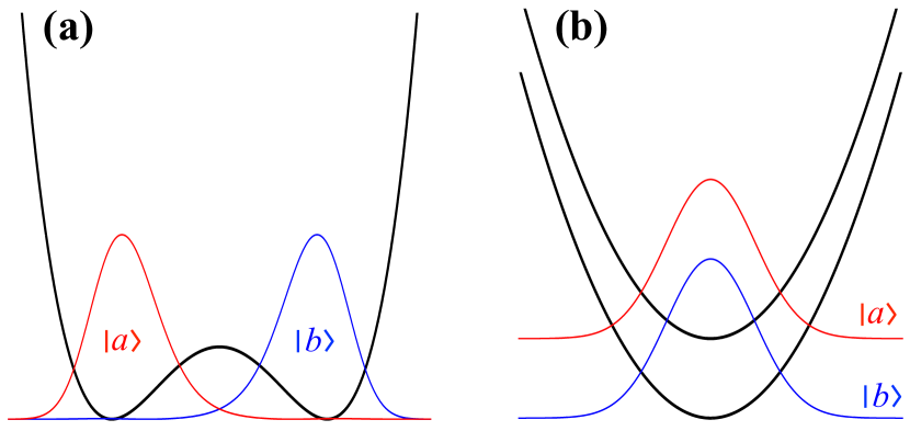
The external bosonic Josephson junction can be realized with a dilute Bose-Einstein condensate confined in a double-well potential Javanainen (1986); Smerzi et al. (1997); Milburn et al. (1997), see Fig. 10(a). For a sufficiently high barrier and weak interaction, we can describe the system in a two-mode approximation. The two modes are given by the first spatially symmetric, , and first antisymmetric, , solutions of the Gross-Pitaevskii equation in the double-well trap Zapata et al. (1998); Raghavan et al. (1999). Spatial modes localized in the left and right well are given by and , respectively, see Fig. 10(a). The parameters in Eq. (63) are then identified as Ananikian and Bergeman (2006)
| (64a) | ||||
| (64b) | ||||
where
| (65) |
is the chemical potential (and analogous definition for ), , is the s-wave scattering length (positive for repulsive interactions and negative for attractive interactions) and is the atomic mass. In the derivation of Eq. (63) we have taken real and normalized to one, and assumed , which is valid for a sufficiently high tunneling barrier.
Experimentally, the external weak link has been realized on atom chips Hall et al. (2007); Schumm et al. (2005); Jo et al. (2007b); LeBlanc et al. (2011); Maussang et al. (2010) as well as in optical traps Shin et al. (2004); Albiez et al. (2005); Hadzibabic et al. (2006). The spatial separation allows for sensing of a variety of fields and forces Cronin et al. (2009); Inguscio and Fallani (2013). The experimental challenges are the required high degree of stability of the external potential, as well as the precise control of the tunneling coupling between the two wells Gati et al. (2006); Levy et al. (2007); Spagnolli et al. (2017).
The internal bosonic Josephson junction is created with a trapped Bose-Einstein condensate in two different hyperfine states Steel and Collett (1998); Cirac et al. (1998), see Fig. 10(b). The Josephson-like coupling is provided by an electromagnetic field that coherently transfers particles between the two states via Rabi rotations Hall et al. (1998a, b); Böhi et al. (2009). Assuming that the external motion of the atoms is not influenced by the internal dynamics, one can apply a single-mode approximation for each atomic species. The many-body Hamiltonian becomes Eq. (63) with coefficients
| (66a) | ||||
| (66b) | ||||
| (66c) | ||||
where is the Rabi frequency, , and are the intra- and inter-species s-wave scattering lengths, and are single-particle mode functions of the two internal states, which can be determined in a mean-field description from the Gross-Pitaevskii equation. A more accurate value for is obtained if one also takes into account the change of the mode functions with particle number, see Li et al. (2008b); Smerzi and Trombettoni (2003). Since the phase and amplitude of the coupling field can be switched on and off on nanosecond time scales, it is possible to implement arbitrary rotations on the Bloch sphere that are helpful to read out and characterize the internal state. Furthermore, during Rabi coupling pulses it is possible to reach the regime , where interaction effects can be neglected.
III.1 Metrologically useful entanglement in the ground state of the bosonic Josephson junction
Several approaches to the bosonic Josephson junction model Hamiltonian (63) have been discussed in the literature. A semiclassical (mean-field) approximation provides useful insights Raghavan et al. (1999); Smerzi et al. (1997). It is obtained by replacing mode operators with complex numbers: and , where and are the numbers of particles and phases of the condensate in the and modes, respectively. The spin operators are replaced by , , and , where is the relative phase between the two condensate modes, and the fractional population difference . The Hamiltonian (63) becomes
| (67) |
where energies are in units of , , and . In the following we mainly focus on the case , unless explicitly stated.
A common method to extend the analysis beyond the mean-field approximation consists of quantizing the conjugate number and phase semiclassical variables Leggett and Sols (1991), i.e., replacing and with operators and obeying the commutation relation , where plays the role of a Planck constant. We can thus write and by canonical quantization. Note that a rigorous phase operator is lacking Carruthers and Nieto (1968); Lynch (1995), and the above phase quantization may break down for large phase fluctuations. Series-expanding Eq. (67) to second order in and we have . By quantizing the conjugate variables we obtain
| (68) |
in number representation, and
| (69) |
in phase representation. Equations (68) and (69) predict Gaussian number and phase ground state wave functions with variances
| (70) |
respectively Paraoanu et al. (2001); Smerzi and Raghavan (2000). Improvements over Eqs. (68) and (69) have been discussed in the literature. Considering a second-order expansion in phase around of Eq. (67) one obtains the Hermitian Hamiltonian
| (71) |
describing a fictitious quantum particle with -dependent effective mass moving in an anharmonic one-dimensional potential
| (72) |
Shchesnovich and Trippenbach (2008) have derived the above Hamiltonian using a continuous approximation of the relative population difference, and avoiding phase-number commutation relations, see also Javanainen and Ivanov (1999); Spekkens and Sipe (1999). For , the effective potential (72) changes from harmonic for , to quartic at , to a double-well shape with wells centered at for . The fictitious quantum particle description is expected to give accurate results for large numbers of particles, provided that the wavefunction is sufficiently smooth and vanishes at the boundaries of Juliá-Díaz et al. (2012), and phase fluctuations remain small. Anglin et al. (2001) proposed a complementary approach consisting of a projection of the bosonic Josephson junction Hamiltonian (63) over the overcomplete Bargmann basis . This leads to an exact quantum phase model , where is an arbitrary two-mode state, is an effective phase wavefunction, and
| (73) |
The first two terms in Eq. (73) give the quantum phase model Hamiltonian that is widely used to study superconducting Josephson junctions Barone and Paternò (1982). The quantum phase model is relevant in the Josephson and Fock regimes, see below. The additional term proportional to is important for weak interactions, in the Rabi regime. Equation (73) is exact in the sense that the lowest frequencies in its eigenspectrum are exactly the spectrum of Eq. (63) Anglin et al. (2001).
Finally, it is worth pointing out that the spectrum of Eq. (63)—and of the more general Lipkin-Meshkov-Glick model—is analytically known in the thermodynamic limit Ribeiro et al. (2007, 2008).
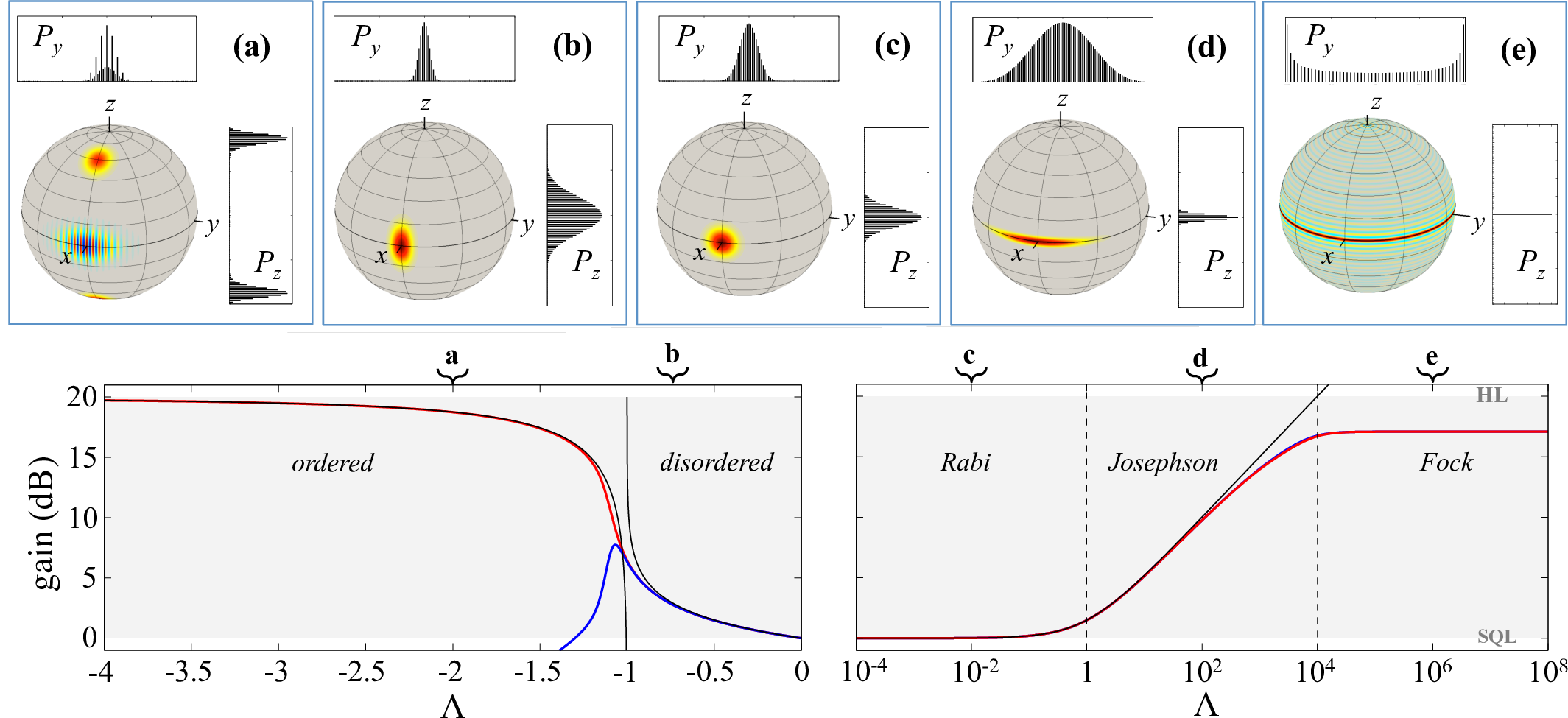
III.1.1 Ground state for positive nonlinearities
A positive effective nonlinearity () makes number fluctuations between the two modes energetically unfavorable. The ground state of Eq. (63) with is thus characterized by a squeezed atom-number distribution at the expense of increased phase fluctuations Leggett and Sols (1998); Javanainen and Ivanov (1999); Spekkens and Sipe (1999); Steel and Collett (1998). Following Leggett (2001), we distinguish three regimes, see Fig. 11.
Rabi regime, .
At the ground state is given by the coherent spin state pointing in the positive- direction (for ), , with binomial occupation of each mode, where is the vacuum. In the Rabi regime, the Josephson junction is dominated by tunneling, which keeps a well-defined relative phase between the two modes. The coherence is high, , and number (phase) fluctuations slightly decrease (increase) with respect to the noninteracting case. Using , and Eq. (70), we find
| (74) |
In particular, in this regime.121212In Eqs. (74)-(77), i.e., for positive nonlinearities, the spin squeezing is calculated as . For negative nonlinearities, Eq. (78), as . The ground state of Eq. (63) is spin-squeezed along the axis, and useful for sensing rotations around the axis.
Josephson regime, .
In the Josephson regime number (phase) fluctuations are further reduced (increased) while the coherence remains high. The approximations leading to Eq. (70) are still very good. We thus expect Gaussian number and phase distributions with width and , respectively, giving Pezzè et al. (2005)
| (75) |
For a fixed ratio , we have , predicting a scaling of phase sensitivity , intermediate between the standard quantum limit and the Heisenberg limit.
Fock regime, .
In the Fock regime interaction dominates over tunneling, giving rise to a fragmented Bose-Einstein condensate Spekkens and Sipe (1999); Jääskeläinen et al. (2004). The phase becomes of the order of and the approach leading to Eq. (70) breaks down. The ground state is approximatively obtained by putting an equal number of particles in both modes, with vanishing number fluctuations. For and even values of , we have . In the limit of large but finite , we find
| (76) |
where is any axis on the equatorial plane of the Bloch sphere. In this limit, both and vanish, such the ratio is finite but very sensitive to experimental noise. For odd values of , we have which is spin-squeezed with
| (77) |
III.1.2 Ground state for negative nonlinearities
A negative effective nonlinearity () favors localization of particles in one mode and, in a symmetric Josephson junction (), enhances number fluctuations. The interplay of linear coupling and nonlinear interaction in the Hamiltonian (63) gives rise to a second-order quantum phase transition with discrete symmetry breaking and mean-field critical exponents. This quantum phase transition is due to the competition between interaction and coupling Ulyanov and Zaslavskii (1992); Botet et al. (1982); Gilmore and Feng (1978), and occurs in the thermodynamic limit, and such that . The order parameter is given by the absolute value of the population imbalance, , with in Eq. (72) playing the role of an effective Ginzburg-Landau potential. Entanglement Buonsante et al. (2012); Ma and Wang (2009); Vidal et al. (2004); Orús et al. (2008); Mazzarella et al. (2011) and fluctuations of the order parameter Ziń et al. (2008) approaching the transition point have been extensively studied. This quantum phase transition has been experimentally investigated by Trenkwalder et al. (2016) in a double-well potential. The dynamics following the sudden quench into the vicinity of the quantum critical point (in a two-component Bose gas) has been studied by Nicklas et al. (2015).
Disordered phase, .
The approximations leading to Eq. (70) remain valid also for weak attractive interactions. We thus find phase squeezing and number anti-squeezing Steel and Collett (1998):
| (78) |
The ground state is entangled and useful for sensing rotations around the -axis, see Fig. 11. At the harmonic-oscillator approximation breaks down and Eq. (70) predicts a divergence of number fluctuations. At the transition point one finds .
Ordered phase, .
This phase is characterized by the presence of macroscopic-superposition state Cirac et al. (1998); Ho and Ciobanu (2004); Huang and Moore (2006); Lee (2006). The mean spin length vanishes and spin squeezing is lost, see Fig. 11. For strong nonlinearities, , the ground state is given by the symmetric superposition (i.e., a Schrödinger cat-like state) of states localized on the right and the left wells of the effective double-well Ginzburg-Landau potential for in Eq. (72) Shchesnovich and Trippenbach (2008), giving
| (79) |
For , the ground state is approximatively given by a NOON state and the quantum Fisher information tends toward the ultimate bound . The macroscopic superposition is lost for and infinitesimally-small energy imbalance , breaking the symmetry of .
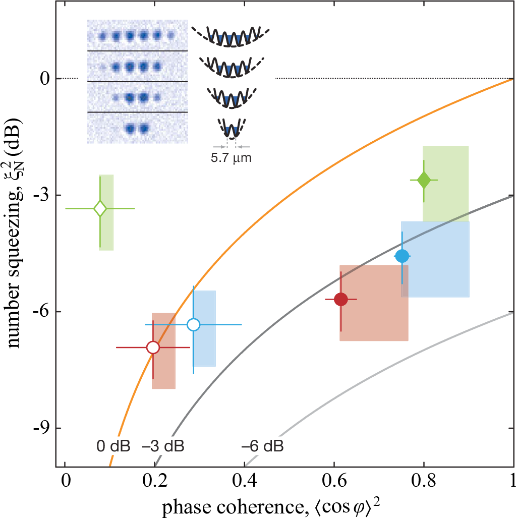

III.1.3 Adiabatic splitting
Experimentally, the Rabi and Josephson regimes for repulsive interactions and the disordered phase for attractive interactions can be reached by adiabatically splitting a Bose-Einstein condensate initially prepared in the ground state of the strong-tunneling (Rabi) regime Javanainen and Ivanov (1999); Menotti et al. (2001); Streltsov et al. (2007); Pezzè et al. (2005); Isella and Ruostekoski (2005); Bodet et al. (2010). By varying the plasma frequency adiabatically in time, the system follows its ground state if Javanainen and Ivanov (1999); Schaff et al. (2014)
| (80) |
Increasing the height of the potential barrier in order to reach the Fock regime, the required timescale for adiabaticity eventually diverges, setting a limit to the attainable entanglement. Shortcut to adiabaticity Lapert et al. (2012); Yuste et al. (2013); Juliá-Díaz et al. (2012) and optimal control techniques Grond et al. (2009); Huang and Moore (2008); Pichler et al. (2016) for the fast production of highly-entangled states have been also studied. It should be noted that Eq. (80) assumes that the gas is prepared in the ground states configuration. Experimentally, the finite temperature of the gas is the main factor limiting the squeezing via the adiabatic-splitting technique Estève et al. (2008).
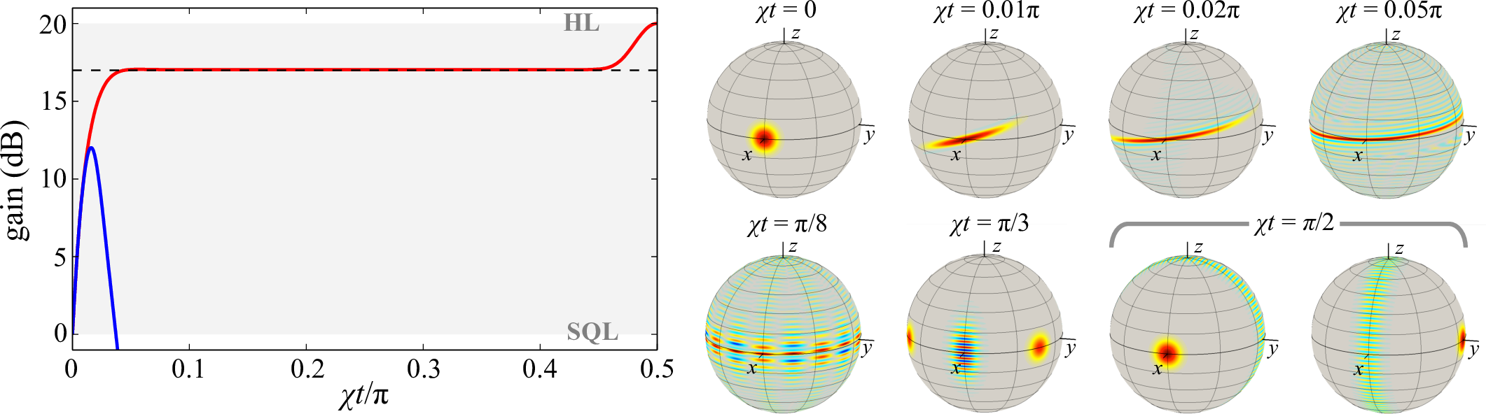
III.1.4 Experimental spin squeezing in the ground state of the BJJ
Estève et al. (2008) reported the first direct experimental demonstration of spin squeezing and entanglement in the ground state of the bosonic Josephson junction. A 87Rb Bose-Einstein condensate confined in a shallow harmonic trap is split adiabatically by ramping up a one-dimensional optical lattice. The particles are distributed over two and six lattice sites, see inset of Fig. 12. Direct atom detection better than atomic shot noise is implemented by absorption imaging of the atomic density, with a spatial resolution well below the lattice spacing. This gives direct access to the number-squeezing parameter . Additionally, the phase coherence is directly obtained from the interference pattern observed after releasing the atomic cloud from the trap. Noticing that (valid for , and ), metrological spin squeezing is given by . The simultaneous presence of number squeezing and high phase coherence allowed to reach an inferred spin squeezing of dB for the two main well pairs of a six-well lattice, and dB for the double-well configuration. The results are summarized in Fig. 12.
More recent experiments have studied number squeezing Maussang et al. (2010) and spin squeezing Berrada et al. (2013) when splitting a Bose-Einstein condensate in a double-well trap on an atom chip. Maussang et al. (2010) realized purely magnetic double-well potential. This experiment reports a detailed investigation of the optimal splitting time, given by the interplay of the barrier raising rate (which must be slow in order to avoid excitations to higher modes), heating effects and atom loss. In Berrada et al. (2013) the splitting is based on radio-frequency dressing Hofferberth et al. (2006) that dynamically deforms the static magnetic trap into a double-well potential Schumm et al. (2005). A split Bose-Einstein condensate of 87Rb atoms is characterized via the measurement of the number of particles in each well and the relative phase, see Fig. 13, showing number squeezing and phase anti-squeezing. From these results, using , it is possible to obtain dB ( dB inferred). This corresponds to a useful (for metrology) entanglement depth of 150 atoms, excluding useful entanglement of less than 67 particles with 90% probability. Berrada et al. (2013) have also investigated the reduced phase diffusion associated to number squeezing Lewenstein and You (1996); Castin and Dalibard (1997); Javanainen and Wilkens (1997) and the fast recombination Jo et al. (2007a); Negretti and Henkel (2004); Negretti et al. (2008); Scott et al. (2008); Berrada et al. (2016) of the condensates in the two wells.
III.2 One-axis twisting dynamics
One-axis twisting is a benchmark model for studying the generation of spin-squeezed states Kitagawa and Ueda (1993), Schrödinger cats Mølmer and Sørensen (1999) and useful entanglement for quantum metrology Pezzè and Smerzi (2009). The one-axis twisting Hamiltonian (here, along the -axis) is
| (81) |
This model can be realized via atom-atom elastic collisions in a Bose-Einstein condensate Sørensen et al. (2001), see Eq. (63), trapped ions, see Sec. VI.2, and cold atoms in an optical cavity, see Sec. V.2.
The quantum dynamics of a localized spin wavepacket can be roughly viewed as a rotation around the axis. The -dependent angular velocity (whose sign differs on the two hemispheres of the Bloch sphere) leads to a twisting of the state on the Bloch sphere. To analyze this effect quantitatively, let us consider the dynamical evolution of an initial coherent spin state pointing along the positive -axis, , see Fig. 14. The coherent spin state initially stretches in the plane tangental to the Bloch sphere. Kitagawa and Ueda (1993) identified the squeezing angle in terms of and , as well as the squeezed and anti-squeezed spin components and , respectively. Squeezing is accompanied by loss of contrast, , as the state spreads on the Bloch sphere. The spin squeezing and the quantum Fisher information are readily calculated, giving Sørensen et al. (2001); Kitagawa and Ueda (1993)
| (82) |
and Pezzè and Smerzi (2009)
| (83) |
respectively.131313The quantum Fisher information optimized over rotation directions in the Bloch sphere is given by the maximum between , Eq. (83), and . For the state is spin squeezed, , reaching at an optimal time . For the states wraps around the Bloch sphere and spin squeezing is lost, . Yet, the state is still entangled. The quantum Fisher information reaches a plateau for signaling entanglement, according to Eq. (32), in the over-squeezed state. The state evolves, at time , into a coherent superposition of coherent spin states distributed evenly on the equator of the Bloch sphere Agarwal et al. (1997), see Fig. 14. At we observe the dynamical creation of a NOON state along the axis, , if is even, and along the axis, , if is odd Agarwal et al. (1997); Mølmer and Sørensen (1999). For the NOON state, the quantum Fisher information, optimized over the spin direction, reaches its maximum value , see Sec. II.3.7. For even (odd) values of , the dynamics is reversed for () and we have a complete revival of the initial condition at (). The one-axis twisting dynamics is modified by particle loss Li et al. (2008a); Sinatra et al. (2011, 2013, 2012); Spehner et al. (2014) and other imperfections such as phase noise Ferrini et al. (2008, 2011) and finite temperature of the Bose gas Sinatra et al. (2011), limiting the achievable squeezing. We will further comment on these works in Sec. VII.


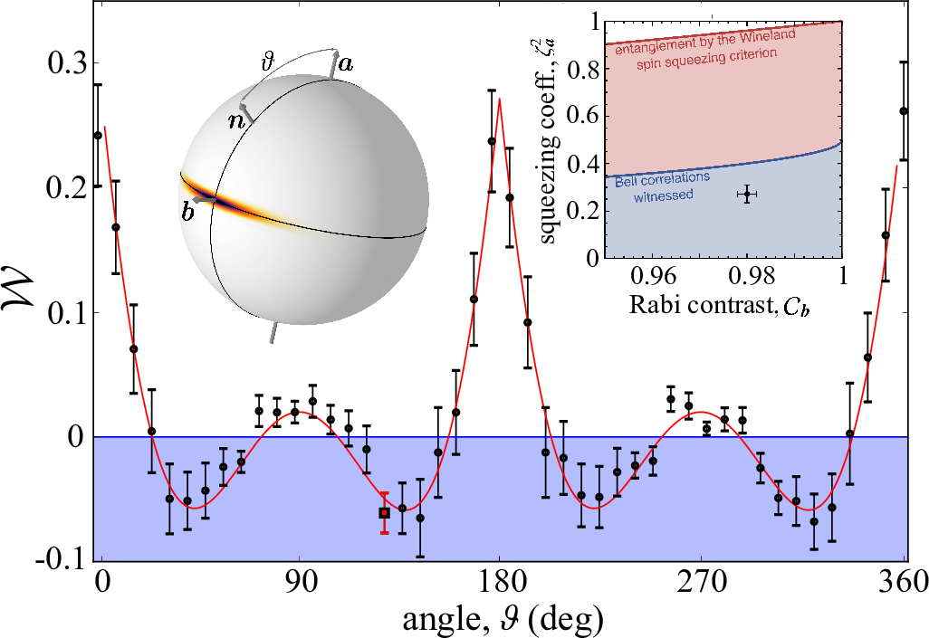
III.2.1 Spin squeezing and particle entanglement
Spin squeezing obtained via one-axis twisting dynamics in a Bose-Einstein condensate has been first experimentally demonstrated by Riedel et al. (2010); Gross et al. (2010). These experiments used a 87Rb condensate prepared in a coherent spin state with equal mean populations in two hyperfine states. With 87Rb atoms, the interaction parameter , see Eq. 66b, is small due to an almost perfect compensation of inter- and intra-species collisional interactions, i.e., . Different approaches have been used to increase artificially: Riedel et al. (2010) used a state-dependent trapping potential to change the wave function overlap between the two internal states and thus reduce Böhi et al. (2009); Li et al. (2008b), while Gross et al. (2010) exploited a Feshbach resonance Chin et al. (2010) to change the scattering length .
Riedel et al. (2010) used a spatially-inhomogeneous microwave field to manipulate the trapping potentials of the atom cloud in the two hyperfine states and by microwave level shifts Treutlein et al. (2006). The trapping potential for atoms in one state is suddenly shifted by such a state-selective force, and the states coherently demix and begin to oscillate in space. In this way the overlap of the wavefunctions of the two states changes dynamically and modulates collisional effects Li et al. (2008b): according to Eq. (66c), when the two components are spatially separated, the inter-species interaction vanishes. The parameter is then determined solely by intra-species interactions and reaches sufficiently-high values to induce fast spin-squeezing dynamics. After each full oscillation, the two states coherently remix and the collisional squeezing dynamics stops. Spin-noise tomography and the reconstructed Wigner distribution of the squeezed state are shown in Fig. 15. The results demonstrate a squeezing parameter dB ( dB inferred). More recent experiments using this technique achieved up to dB with detection noise subtracted Ockeloen et al. (2013); Schmied et al. (2016).
Gross et al. (2010) used a Bose-Einstein condensate of atoms in the and hyperfine levels of the electronic ground state of Rubidium. A bias magnetic field is used to bring the system near a Feshbach resonance, to reduce the inter-species s-wave scattering length and thus enhance the effective nonlinearity leading to squeezing and entanglement. Spin-noise tomography leads to an inferred dB, predicting an entanglement depth excluding less than 80 particles within three standard deviations (and a mean of 170 entangled atoms).
III.2.2 Quantum interferometry
Gross et al. (2010) have also demonstrated a full Ramsey interferometer sequence with spin-squeezed states, see Fig. 16. Squeezed-state creation is followed by a rotation around the axis to prepare a phase-squeezed state (i.e., squeezed along the axis)—in effect constructing a nonlinear beam-splitter. After a short interrogation time , during which the interaction is still active, a second beam splitter closes the Ramsey sequence. The directly measured phase sensitivity gain is dB, corresponding to a reduction of phase variance 15% below the standard quantum limit. In a more recent experiment, Muessel et al. (2014) have been able to scale the generation of spin-squeezed states up to particles using a chain of trapped independent condensates and exploiting a differential estimation of the phase. They demonstrated a spin squeezing dB and a sensitivity 24% below the standard quantum limit. Ramsey interferometry using spin-squeezed states generated via one-axis twisting in Bose-Einstein condensate has recently found application to sense magnetic fields Ockeloen et al. (2013); Muessel et al. (2014), as discussed in more detail in Sec. VII.
III.2.3 Bell correlations
Schmied et al. (2016) have observed Bell correlations in spin-squeezed Bose-Einstein condensates of about 87Rb atoms trapped on an atom chip. Following the generation of the spin-squeezed state by one-axis twisting, the Bell correlation witness of Eq. (57) is determined by measuring the second spin moment along the squeezed direction and combining it with spin contrast measurements along other projection axes, see Fig. 17. The measured values of violate the inequality (57) and thus also the inequalities (58) and (59). This proves the presence of Bell correlations and implies that the spin-squeezed states can violate the many-particle Bell inequality of Tura et al. (2014). The detection of Bell correlations indicates that spin-squeezed states are useful beyond quantum metrology: they also contain the resource for quantum information tasks such as certified randomness generation or quantum key distribution Brunner et al. (2014).
While Schmied et al. (2016) observed Bell correlations in a spin-squeezed BEC, Engelsen et al. (2017) have confirmed Bell correlations in a spin-squeezed thermal ensemble. The interpretation of these experiments relies on the common assumption that atoms do not communicate through unknown channels. This assumption can be relaxed if the atoms are spatially separated in an optical lattice potential, as proposed in Pelisson et al. (2016). Many-body Bell tests with Bose-Einstein condensates have also been proposed in Mullin and Laloë (2008); Laloë and Mullin (2009). In section III.4 we discuss proposals to create entanglement between spatially separated spinor condensates, which could also be employed for Bell tests.
III.3 Twist-and-turn dynamics
The creation of entanglement in the one-axis twisting model is enriched—and accelerated, to some extent Muessel et al. (2015); Sorelli et al. (2015)—by the dynamical evolution using the turning term simultaneously with the twisting term in the Hamiltonian (63). The resulting twist-and-turn dynamics is experimentally studied from the starting point of a coherent spin state pointing in the or direction. The interaction is suddenly switched to a finite value of in presence of linear coupling.
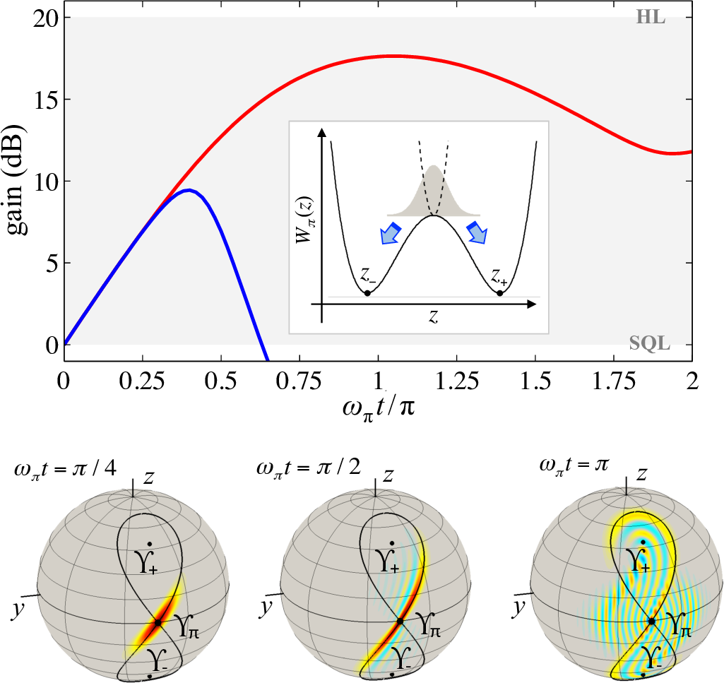
The twist-and-turn can be described as the dynamics of an effective relative-number wavepacket Juliá-Díaz et al. (2012). For an initial coherent spin state polarized along the positive -axis, the effective Hamiltonian is given by Eq. (71). can be well approximated as a harmonic potential of frequency . Suddenly switching the interaction from to a positive value (corresponding a tighter the harmonic oscillator potential, i.e., ) gives rise to a breathing mode of the effective wavepacket with periodic squeezing of the relative population. For a coherent spin state polarized along the negative -axis, the effective Hamiltonian is with . For , is harmonic with frequency . Since , a sudden switch of the interaction leads to a breathing motion predicting number anti-squeezing (and phase squeezing). Damping of the oscillations is observed for increasing values of Choi and Bigelow (2005); Gordon and Savage (1999) corresponding to the wavepacket feeling the anharmonicity of the effective potential.
These predictions are recovered, for , by a frozen-spin approximation Law et al. (2001) that consists of neglecting fluctuations of the mean spin, being replaced by . The variances
| (84a) | ||||
| (84b) | ||||
show periodic oscillations and the spin-squeezing parameter reaches () for the coherent spin state pointing along the positive (negative) axis.
The situation changes completely if Micheli et al. (2003); Gordon and Savage (1999). The potential turns from a single-well to a double-well shape, with minima at . The initial coherent spin state corresponds to a Gaussian wavepacket that sits at the top of the double-well barrier, see Fig. 18. The repulsive potential tends to split the state giving rise to a macroscopic superposition corresponding to the wavepacket localized in the left and right well of . The semiclassical equations of motion and , where is given by Eq. (67), offer an alternative view Smerzi et al. (1997); Raghavan et al. (1999). The fixed point becomes unstable for and two new stable fixed points appear. The exact quantum dynamics shows that, at short times, the state stretches along the semiclassical separatrix passing through , see Fig. 18. At longer times the quantum state wraps around . In this regime, spin squeezing is lost, while the quantum Fisher information—sensitive to the creation of macroscopic superposition of states—continues increasing. For the semiclassical separatrix reaches the poles of the Bloch sphere: the dynamics creates NOON-like states on a time scale Micheli et al. (2003). For the separatrix winds around the Bloch sphere, the maximum distance between the separatrix and the equator decreases, and the dynamics resembles that of the one-axis twisting.

III.3.1 Entanglement beyond spin squeezing
Twist-and-turn dynamics has been investigated by Strobel et al. (2014); Muessel et al. (2015) using two internal hyperfine levels and of 87Rb atoms. A narrow Feshbach resonance is used to reduce the inter-species interaction. Coupling between the internal levels is provided by radiofrequency and microwave drive. The experiments start with atoms in the mode, followed by a Rabi pulse that prepares a coherent spin state aligned with the -axis. Subsequently, the Rabi coupling is decreased to reach , and its phase adjusted to orient it along the negative -axis. Muessel et al. (2015); Strobel et al. (2014) have investigated the short-time spin-squeezing dynamics. For an evolution of 15 ms, Strobel et al. (2014) demonstrated dB [and inferred dB Muessel et al. (2015)]. Muessel et al. (2015) also demonstrated a spin squeezing dB using 30 independent condensates in parallel (each condensate experiencing independently a twist-and-turn dynamics), with a total of particles. For longer times, spin squeezing is quickly lost and the experimental Husimi distribution of the reconstructed state shows the characteristic S-shape, see Fig. 19. Strobel et al. (2014) extracted the Fisher information using a “Hellinger method”, reaching values and thus demonstrating that the state is entangled. The experimental extraction of the Fisher information requires to rotate the state around the -axis, and to collect the probability distributions of the relative particle number in and at different rotation angles. The Fisher information is obtained from a quadratic fit of the Hellinger distance (17), according to Eq. (18), between a reference distribution (at ) and the distribution obtained at a finite . Experimental results are shown in Fig. 19.
III.4 Entanglement of two spatially-separated spinor Bose-Einstein condensates
Creating entanglement between two spatially separated—individually addressable—spinor Bose-Einstein condensates offers interesting possibilities: in such a system, local manipulations and measurements can be performed on the spin state of each condensate separately and nonlocal quantum correlations between the measurement results can be directly observed. This is particularly relevant for experiments on EPR entanglement and Bell tests, where the spatial separation can be used to rule out unknown causal influences between the clouds.
He et al. (2011b); Bar-Gill et al. (2011); Kurkjian et al. (2013) have proposed schemes to generate EPR entanglement between two spatially separated Bose-Einstein condensates using elastic collisions. The condensates represent collective spins and , respectively, which can be individually addressed and prepared in a coherent spin state. He et al. (2011b); Bar-Gill et al. (2011) have considered schemes where EPR entanglement is generated by first spin-squeezing each condensate and then interfering the squeezed states on a beam splitter. In the scheme of Kurkjian et al. (2013), on the other hand, a state-dependent potential is turned on such that the wave function of state of the first condensate overlaps with the wave function of state of the second condensate, picking up a collisional phase shift. Dropping constant and linear terms in , this realizes the Hamiltonian , which generates entanglement between the two condensates in addition to spin-squeezing in each condensate. After an interaction time, the state-dependent potential is turned off and the condensates are spatially separated again for detection, revealing EPR entanglement between them Kurkjian et al. (2013). For long interaction times, macroscopic entangled states can be created, as also analyzed by Byrnes (2013), who investigated applications of entangled Bose-Einstein condensates in quantum information processing Byrnes et al. (2012). While such experiments have not yet been reported, we note that continuous-variable entanglement has been created between spatially separated atomic vapor cells using a measurement-based scheme Julsgaard et al. (2001).
IV Entanglement via atomic collisions: spin-mixing dynamics
The generation of correlated photon pairs via spontaneous parametric down-conversion in nonlinear crystals Kwiat et al. (1995) is one of the most widely used sources of entangled quantum states in optics O’Brien et al. (2009). When post-selecting photons in the pair distribution (let us indicate with the signal and idler modes), the corresponding state is a twin-Fock, . The twin-Fock state has been used to overcome the standard quantum limit in an optical interferometer using up to photons per pair Krischek et al. (2011); Nagata et al. (2007); Xiang et al. (2011). Without post-selection, parametric down-conversion creates quadrature-squeezed light Walls (1983); Wu et al. (1986); Slusher et al. (1985); Breitenbach et al. (1997); Ou et al. (1992). Following the proposal of Caves (1981), squeezed light has been successfully used for optical interferometry beyond the standard quantum limit Vahlbruch et al. (2005, 2016), with direct application to gravitational wave detectors Aasi et al. (2013); Schnabel et al. (2010). In the same spirit, the generation of correlated pairs of atoms has thus attracted large interest: many experiments have been proposed and performed. In the following, we review the most successful of these techniques, namely, spin-mixing dynamics in a spinor Bose-Einstein condensate Stamper-Kurn and Ueda (2013); Kawaguchi and Ueda (2012), see Sec. IV.1. We discuss the creation of twin-Fock states in Sec. IV.2, and quadrature squeezing in Sec. IV.3. Finally, in Sec. IV.4 we review alternative protocols for the creation of atom pairs.
IV.1 Spinor Bose-Einstein condensates
IV.1.1 Spin-changing collisions
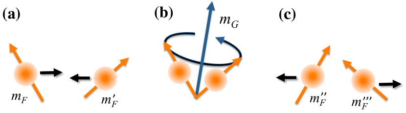
When a Bose-Einstein condensate is confined in a far-off resonant optical dipole trap, the spin degree of freedom of the atoms evolves freely: spin-changing s-wave collisions, see Fig. 20, give rise to a coherent redistribution of atomic populations among Zeeman sub-levels while preserving the total magnetization Ho (1998); Ohmi and Machida (1998). The quantum description of an ultracold gas of spin- bosons requires introducing a vector order parameter with components, Stamper-Kurn and Ueda (2013); Kawaguchi and Ueda (2012). Here is the atomic field annihilation operator associated with the hyperfine spin state . The single-mode approximation Law et al. (1998) assumes that the spatial atomic density distribution of all spin components is approximately equal, and not affected by the spin dynamics. The common scalar wavefunction defining the spatial mode of the condensate is determined as the solution of the Gross-Pitaevskii equation, neglecting contributions from the spin-dependent interactions. In this approximation, the field operators are , where are annihilation operators that obey the usual bosonic commutation relations. We define as the number of particles in the mode , and the total number of particles. The many-body Hamiltonian for a Bose-Einstein condensate is Law et al. (1998); Pu et al. (1999)
| (85) |
where we have neglected terms proportional to the conserved magnetization (we assume in the following) and total number of atoms. Here, is an effective quadratic Zeeman shift, where is the relative energy shift of the mode, which can be tuned by a magnetic field ( being proportional to the square of the magnetic field) and/or near-resonant microwave dressing. The interaction parameter is , with , and the scattering lengths for s-wave collisions in the allowed channels. The single-mode approximation is valid if the system size is much smaller than the spin healing length, , where is the density of the component, giving the minimum size of a spin-domain Stamper-Kurn and Ueda (2013). The last term in Eq. (85) describes the coherent and reversible creation of a pair of atoms in the magnetic sublevels from the scattering of two atoms in .
It is useful to rewrite the Hamiltonian (85) in terms of the spin operators
| (86) |
where and are symmetric and antisymmetric combinations of and . The spin operators and do not commute with each other, and define two SU(2) subspaces. With these operators, the Hamiltonian (85) takes the compact form Duan et al. (2002)
| (87) |
which highlights the presence of nonlinear spin terms. It should be noticed that a symmetric radio-frequency coupling between the modes with Rabi frequency corresponds to a rotation of the vector around the axis, . A relative phase shift between the and modes corresponds to a rotation of both and around the axis, .
Another popular expression of Eq. (85) is Law et al. (1998); Zhang and Duan (2013)
| (88) |
where , , and obey angular momentum commutation relations.141414Some authors have also studied spin-1 condensates using the a quadrupole tensor operator Hamley et al. (2012); Sau et al. (2010); Müstecaplıoğlu et al. (2002) with components related to Eq. (IV.1.1) as , , , and .
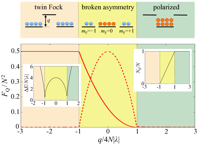
IV.1.2 Ground state of the spin-mixing Hamiltonian
The ground state of the Hamiltonian (85) is characterized by the competition between the energy shift, proportional to , and the spin-dependent collisional interaction, proportional to Lamacraft (2007); Murata et al. (2007); Sadler et al. (2006). The mean-field limit of Eq. (85), obtained by replacing and assuming , gives , where Zhang et al. (2005); Stamper-Kurn and Ueda (2013). In a full quantum treatment, the system is conveniently studied in the Fock basis , where indicates a state of particles in the mode , or in terms of the eigenstates (here ) of and Law et al. (1998).
For a ferromagnetic condensate, (e.g., 87Rb) there are two quantum phase transitions with order parameter given by the mean population of the mode. For , the ground state is , corresponding to a polar phase with all particles in (). For , the minimization leads to and , corresponding to the co-called broken asymmetry phase. The population of decreases linearly with and are (equally) populated. For , we have a twin-Fock phase with and the ground state given by the twin-Fock state . Entanglement in the ground state for the spin-1 system has been studied by Zhang and Duan (2013). Feldmann et al. (2018) have studied the quantum Fisher information of the ground state of the Hamiltonian (85) for different operators. In particular, at Zou et al. (2018), associated to the presence of macroscopic superposition states Pezzè et al. (2017), and in the twin-Fock phase, see Fig. 21, where and .
For an anti-ferromagnetic condensate, (e.g., 23Na)., the mean field energy is minimized by taking and for , and for . There is a quantum phase transition at . In the limit , for the ground state is given by the fully polarized state , while for by the twin-Fock state . See Wu and You (2016) for a calculation of the quantum Fisher information of the ground state for and nonzero magnetization.
IV.1.3 Quantum spin-mixing dynamics in the low-depletion limit
The spin dynamics of an initial condensate in is formally analogous to optical spontaneous four-wave mixing Goldstein and Meystre (1999): atom-atom interaction plays the role of the nonlinear Kerr medium, the condensate is equivalent to a coherent pump field with the external trapping potential corresponding to a high-finesse cavity, and the condensates in can be identified as signal and idler. Remarkably, spin changing collisions are unaffected by the linear Zeeman shift from a homogeneous magnetic field. Only higher-order effects, such as a quadratic Zeeman shift or a linear Zeeman shift from an inhomogeneous magnetic field, affect it.
The low-depletion limit, i.e., , is analyzed by replacing the mode operator in Eq. (85) with . In this approximation, the condensate serves as an unlimited particle resource for the parametric amplification of the modes. We obtain the quadratic Hamiltonian , where and , that can be diagonalized by a Bogoliubov transformation Duan et al. (2000b); Pu and Meystre (2000), see also Truax (1985). The unitary evolution can be calculated exactly, giving
| (89) |
where , and indicates empty modes. This state has a vanishing population difference , while the modes are nonempty, , and characterized by large (super-Poissonian) population fluctuations, . It is also interesting to consider the quadratures
| (90a) | ||||
| (90b) | ||||
where , , , and an analogous definitions of in terms of the operators and introduced above. The time-dependent coefficients are and .
For , is imaginary and the condensate is dynamically unstable. The instability is characterized by the exponential increase of population in the modes, . On resonance () the spin-mixing Hamiltonian becomes , which generates the familiar two-mode squeezed-vacuum state Walls and Milburn (1994),
| (91) |
where and . The Hamiltonian (for ) can be rewritten using the operators and as , which generates a single-mode squeezed-vacuum Walls and Milburn (1994) in each mode. It can also be rewritten as , corresponding to two-axis counter-twisting Kitagawa and Ueda (1993); Duan et al. (2002); Anders et al. (2018) for the and spins. Note that and commute in the low-depletion limit. For , Eq. (90a) reduces to , and Eq. (90b) to . The quadrature [] is squeezed by a factor below the vacuum level at an optimal angle [], and anti-squeezed by a factor at []. For a sufficiently long evolution time, spin dynamics is modified by the depletion of the condensate. The initially exponential growth of population in slows down and finally stops Law et al. (1998); Mias et al. (2008)
For the spin-mixing dynamics is stable and the population of oscillates in time, . For the amplitude of this oscillation becomes negligible and the system remains stable in .
Typical experiments exploring the quantum spin-mixing dynamics Leslie et al. (2009); Liu et al. (2009); Klempt et al. (2010); Chang et al. (2005); Schmaljohann et al. (2004); Peise et al. (2015b) start with a condensate in the stable configuration. A sudden quench brings the condensate in the dynamical unstable configuration. After spin-mixing dynamics, the trap is turned off and a Stern-Gerlach field is used to separate the components during a time-of-flight expansion.
IV.2 Population correlations and twin-Fock state
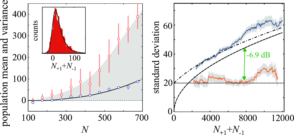

Several experiments have explored the creation of the twin-Fock state in the Zeeman modes. This can be accessed either by quantum spin-mixing dynamics (which can turn a large fraction of an atomic Bose-Einstein condensate into a mixture of perfectly correlated pairs of atom, with large fluctuations of ) or by adiabatic preparation. The twin-Fock state is particle entangled and useful in a Ramsey interferometer to reach sensitivities beyond the standard quantum limit, see Sec. II.3.6.
IV.2.1 Number squeezing
The presence of correlations in the populations of states after spin dynamics has been first demonstrated by Bookjans et al. (2011); Lücke et al. (2011); Gross et al. (2011). Number squeezing up to dB [ dB has been reported more recently by Lücke et al. (2014)] below the projection noise level has been reported, see Figs. 22. The main limitation is given by detection noise for short-time evolutions, and particles losses for long time.
IV.2.2 Quantum interferometry with twin-Fock states
Lücke et al. (2011) have investigated the phase sensitivity of the paired atoms. The experimental sequence starts with the spin-mixing dynamics of a 87Rb condensate prepared in . The generated atom pairs in (due to the short evolution time, the populations in can be neglected due to the quadratic Zeeman shift detuning) are coupled via a series of microwave pulses of variable duration, see Fig. 23. This forms an internal-state beam splitter , where the rotation angle is estimated via the measurement of . The output state is post-selected to a total number . Ideally, this post-selection would correspond to a twin-Fock state as input of the beam splitter operation. Applying error propagation , it was possible to demonstrate a sensitivity 1.61 dB below the standard quantum limit at an optimal rotation angle, see Fig. 23.
IV.2.3 Particle entanglement
Lücke et al. (2014) have investigated particle entanglement in the atomic twin-Fock state. After spin-mixing dynamics of a 87Rb condensate, the number of particles in is post-selected for a total number of . Entanglement is witnessed by the inequality , Eq. (49), further extended to detect an arbitrary -particle entanglement Lücke et al. (2014). Experimental data exclude an entanglement depth of less than 28 atoms with two standard deviations of confidence, and show an average entanglement depth of 68 atoms. It should be noted that signals entanglement independently from its metrological usefulness. Useful -particle entanglement is a more demanding resource than algebraic -particle entanglement: in Apellaniz et al. (2015), similar experimental data as those reported by Lücke et al. (2014) show a useful entanglement depth of about 3 atoms.
IV.2.4 Adiabatic state preparation
Twin-Fock states can be accessed, for an initial condensate prepared in at high values, via an adiabatic passage through the quantum phase transition(s) Zhang and Duan (2013); Luo et al. (2017) discussed in Sec. IV.1.2. The ferromagnetic condensate is favorable since the energy gap closes as , while the energy gap for the anti-ferromagnetic condensate closes as . The condensate is initially prepared via optical pumping with all atoms in and, ideally, an adiabatic ramp of would transform the polarized state to a twin-Fock state with atoms in Zhang and Duan (2013). Hoang et al. (2016) have characterized the amplitude excitations and measured the energy gap of the quantum phase transition in a 87Rb condensate. The entangled state preparation has been experimentally investigated by Luo et al. (2017) for a 87Rb condensate of atoms. This experiment demonstrates—despite the diabatic ramp of the parameter and the finite loss rate—a deterministic and almost perfect conversion to the modes [ at the end of the ramp], high squeezing [ dB] and high coherence. The measurements demonstrate an average entanglement depth of atoms, with more than atoms at the confidence level of one standard deviation. In a successive experiment, Zou et al. (2018) have investigated the adiabatic preparation of the ground state at , corresponding to a spin-1 Dicke state of the manifold. The prepared state has been used to estimate the angle of a Rabi rotation with a sensitivity 2.42 dB beyond the standard quantum limit.
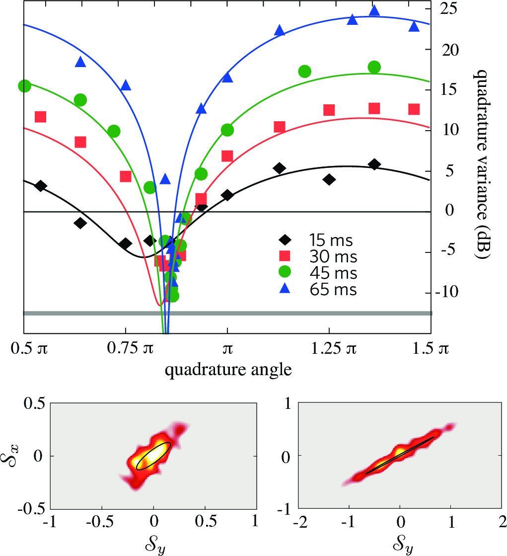
IV.3 Quadrature squeezing and squeezed-vacuum state
IV.3.1 Quadrature squeezing
The experiments of Hamley et al. (2012); Gross et al. (2011); Peise et al. (2015a) have investigated quadrature squeezing in the state generated via spin-mixing dynamics in the low-depletion limit. In this regime, the quadrature variance Eq. (90a) can be rewritten as and [and analogous relation between Eq. (90b) and the spin]: quadrature squeezing thus corresponds to spin squeezing. Experimentally, the quadrature modes are accessed via atomic homodyne detection first realized by Gross et al. (2011), see also Peise et al. (2015a). In analogy to standard techniques in quantum optics Scully and Zubairy (1997); Ou et al. (1992), it consists of a symmetric radiofrequency coupling between the modes. In the limit of low transfer and , this corresponds to a displacement operation, where the condensate in is used as local oscillator. Hamley et al. (2012) have used 87Rb atoms and characterized the spin-squeezed states via noise tomography, see Fig. 24. Values up to dB ( dB inferred) below the SQL are reported.
IV.3.2 Continuous variable and EPR entanglement

The two-mode squeezed-vacuum state (91) realizes—in field modes—the position-momentum correlations that are at the heart of the Einstein-Podolsky-Rosen (EPR) criterion Reid (1989), see Sec. II.3.9. We recall that151515Notice the relations and , where . In particular and . . As the angle is varied, these quadrature variances oscillate between a maximum value and a minimum value , which is below the value of 1 of the unsqueezed vacuum state. In the limit , at (), we have perfect correlations between and ( and ), as well as between and ( and ), where . According to the criteria (55) and (56) discussed in Sec. II.3.9, the two-mode squeezed-vacuum state produced via spin-mixing dynamics in spinor condensates Duan et al. (2000b); Pu and Meystre (2000) is mode entangled for and fulfills the EPR criterion for Reid et al. (2009). 161616In the case of a finite number of particles in the mode Ferris et al. (2008); Raymer et al. (2003), the inequalities (55) and (56) generalize to , and , respectively. The quadratures are proportional to the number of particles measured after a radiofrequency pulse coupling with Gross et al. (2011). With spinor condensates Duan et al. (2002), continuos variable entanglement, e.g., the violation of Eq. (55), was first demonstrated by Gross et al. (2011), while EPR entanglement, e.g., the violation of Eq. (56) was observed by Peise et al. (2015a), see Fig. 25. The experimental violation of Eq. (56) demonstrates a form of entanglement intrinsically connected with local realism. The demonstration of the continuous-variable EPR paradox with massive particles would additionally require space-like separation of measurements to rule out causal influences, which has not yet been experimentally achieved.
IV.3.3 Interferometry with squeezed vacuum
Quadrature squeezing is a resource for quantum interferometry, see Sec. II.3.5. Within spin-mixing dynamics, squeezing occurs in the quadratures corresponding to the symmetric and the anti-symmetric combinations of the modes. Kruse et al. (2016) have realized an atomic clock that exploits the squeezed-vacuum states created in the mode. An initial condensate of atoms undergoes spin-mixing dynamics in the manifold of 87Rb, in the low-depletion regime ( after spin dynamics). The interferometer consists of a rf coupling (corresponding to a balanced beam splitter between the condensate in and the squeezed vacuum in , ), a relative phase shift implemented by a detuned pulse between and , and a second balanced beam splitter between and . The anti-symmetric mode is left unchanged by the interferometer transformation (up to an overall phase), while the is rotated in the Bloch sphere identified by the manifold. The experiment of Kruse et al. (2016) reports Ramsey fringes as a function of reaching a clock sensitivity 2.05 dB below . In the absence of noise, the expected sensitivity is Caves (1981) in the low squeezing regime, and can reach the Heisenberg limit when the input states have the same population on average Pezzè and Smerzi (2008).
IV.3.4 Nonlinear SU(1,1) interferometry
Spin-mixing dynamics can be also used to realize a SU(1,1) interferometer, as first proposed by Yurke et al. (1986) in optics [recently realized with a bright laser source by Hudelist et al. (2014) and with a hybrid atom-light system by Chen et al. (2015a)] and further analyzed by Marino et al. (2012); Gabbrielli et al. (2015) for spinor condensates. The basic idea of this interferometric scheme is to replace the linear beam splitters of a standard Mach-Zehnder scheme with nonlinear beam splitters that create/annihilate pairs of particles, as implemented via spin-mixing dynamics. Let us indicate with the total average number of atoms transferred in pairs from a condensate prepared in to the initially empty modes. After spin mixing, the system acquires a relative phase between and modes. A second spin-mixing dynamics closes the interferometer. The final populations in depend on . When treating the condensate in as an undepletable source of atomic pairs, the predicted phase sensitivity is Yurke et al. (1986)
| (92) |
Equation (92) reaches at the optimal working point (a dark fringe, where no particle is found in the output states) and shows that only the particles outcoupled from the mode contribute to the phase sensitivity.
An analysis beyond the low-depletion limit shows that the SU(1,1) interferometer scheme can overcome the standard quantum limit with respect to the total number of particles in the initial condensate Gabbrielli et al. (2015) and reach . The sensitivity can be further enhanced by an additional linear coupling of the three modes before and after phase imprinting, a scheme called “pumped-up” SU(1,1) interferometer Szigeti et al. (2017).
Linnemann et al. (2016) have experimentally realized a nonlinear SU(1,1) interferometer within the manifold of 87Rb. The experiment is performed in the low-depletion regime, , using atoms. The interferometer is probed by tuning the relative phase between the condensate and the modes to the dark fringe. The phase is imprinted via a second-order Zeeman shift by applying a magnetic field for varying times, and is read out from the mean total number of atoms in the modes. Results demonstrate a sensitivity close to the theoretical prediction of Eq. (92).
IV.4 Other protocols to create correlated atomic pairs
Spin-mixing dynamics is not the only possibility to create correlated atom pairs. Alternative methods have been studied and implemented experimentally. Relative number squeezing between two outgoing Bose-Einstein condensates with opposite momenta was obtained in the collisional de-excitation of a one-dimensional quasi-condensate, where the reduced dimensionality restricted the number of available modes Bücker et al. (2011). The atoms are initially prepared in a highly non-equilibrium state such that the only allowed de-excitation channel is a two-particle collision process, emitting atom pairs. Bücker et al. (2011) observed a number squeezing of up to dB. Jaskula et al. (2010) observed sub-Poissonian atom number fluctuations, with 0.5 dB of number squeezing, between outgoing modes of opposing momenta in the halo produced by the s-wave scattering of two Bose-Einstein condensates of metastable 4He. The amount of detected squeezing was limited by the large number of outgoing collisional modes (isotropically distributed over the scattering sphere) and the correspondingly small number of atoms per mode. With the same scheme Lewis-Swan and Kheruntsyan (2014) it was possible to demonstrate Hong-Ou-Mandel interference Hong et al. (1987). Each atom of the pair is in the motional degree of freedom is sent to the input channel of a beam splitter realized using Bragg scattering on an optical lattice Bonneau et al. (2013). When two inputs are indistinguishable, they emerge together in one of the output channels, demonstrating two-particle interference Lopes et al. (2015).
V Entanglement creation via atom-light interaction
The light-matter quantum interface finds important applications in several areas of quantum information processing Hammerer et al. (2010); Kimble (2008). Here we review the many successful experiments and proposals that exploit the coupling between atoms and light for the creation of useful entangled states for quantum metrology. This quest started in the late 1990s with pioneering experiments using room-temperature vapor cells Kuzmich et al. (1999, 2000) and laser-cooled atomic gases Hald et al. (1999), which demonstrated the reduction of atomic spin (or pseudospin) fluctuations. In these experiments, the atom-light interface was implemented in free space using optically-thick atomic ensembles Kuzmich and Polzik (2003). Optical cavities can be used to effectively increase the optical depth of the atomic sample and represent a versatile system with rich possibilities for creating entanglement between atoms Miller et al. (2005); Tanji-Suzuki et al. (2011); Ritsch et al. (2013). These techniques have allowed the demonstration of metrological spin-squeezing, squeezed-state atomic clocks and the creation of highly non-classical states.
Key theoretical proposals and experiments on atom-light interfaces for quantum metrology can be classified in three broad categories: (a) nondestructive measurements, including quantum nondemolition measurements and Zeno dynamics, Sec. V.1; (b) light-mediated coherent interaction between distant atoms, Sec. V.2; and (c) transfer of squeezing to atoms via absorption of non-classical light, Sec. V.3. Atom-light interaction currently represents the most successful method for producing large amounts of squeezing and entanglement in atomic ensembles.
V.1 Quantum state preparation using nondestructive measurements
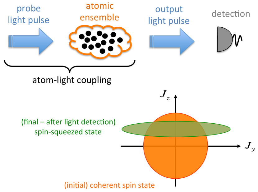
V.1.1 Quantum nondemolition measurements in free space
In a quantum nondemolition (QND) measurement, a system (e.g., an atomic cloud) and meter (a measurement degree of freedom, e.g., a light beam) are coupled, such that a direct measurement of the meter provides indirect information about an observable of the system Braginsky et al. (1980); Braginsky and Khalili (1992); Grangier et al. (1998). The measurement is called QND if the system and the measured value of the observable are conserved after the measurement. QND measurements are a resource for quantum metrology as they allow the preparation of entangled and spin-squeezed states of many atoms. This is well illustrated by a model Hamiltonian describing a far-off resonant dispersive interaction between the collective spin of an ensemble of atoms and a two-mode light beam in free space Kuzmich et al. (1998); Takahashi et al. (1999):
| (93) |
Here, is the light pulse duration, is the atomic collective spin, and is the Stokes vector operator of the light, with components , , and . can be two polarization modes Takahashi et al. (1999); Hammerer et al. (2004), in which case Eq. (93) describes the paramagnetic Faraday rotation of light; they can also be two spatial modes of an optical Mach-Zehnder interferometer where atoms are placed in one arm and phase-shift the light Oblak et al. (2005); Chaudhury et al. (2006); Windpassinger et al. (2008). The dimensionless interaction strength in Eq. (93) is , where is the resonant photon scattering cross section of the probe transition, is the spontaneous emission rate, is the spatial cross section of the atomic ensemble illuminated by the pulse, and the detuning of the light from resonance Hammerer et al. (2010). The Hamiltonian (93) satisfies the back-action evasion condition such that is a constant of motion. During the interaction, precesses around the -axis by an angle . To lowest order in this angle, we have
| (94a) | |||
| (94b) | |||
| (94c) | |||
A measurement of or thus realizes a QND measurement of while preserving the system’s quantum coherence. As an illustration, we take atomic and optical systems both initially prepared in coherent spin states polarized along the -axis. Assuming and , the average phase precession is zero, , while the variance increases with , where is the number of atoms, and the number of photons in the pulse. The mean value and variance of after the measurement of the light spin (with result ) are
| (95a) | ||||
| (95b) | ||||
respectively, see Fig. 26. Although the final atomic state depends on the result of the measurement of the light beam (and it is thus termed conditional), the reduction in spin noise according to Eq. (95b) is completely deterministic, with no post-selection necessary. Unconditional spin squeezing can be achieved via quantum feedback that compensates, via a spin rotation, the stochastic shift of in Eq. (95a) due to the random measurement outcome Thomsen et al. (2002); Berry and Sanders (2002). Inoue et al. (2013); Cox et al. (2016) have experimentally demonstrated such unconditional spin squeezing via feedback control, see also Vanderbruggen et al. (2013). In the QND scheme, the squeezing is due to the projective measurement of the atomic state upon detection of the light, and its efficacy is determined by the performance of the detector. Yet, the above discussion is highly idealized: far-off resonant dispersive probing is unavoidably accompanied by decoherence due to Raman spin flips.171717In the literature, non-ideal measurements are still termed QND provided that the loss of coherence in the atomic ensemble remains small. Notice that , where is the resonant optical depth and is the average photon scattering rate per atom during the probe pulse. Scattered photons carry information about the spin state of the atoms: these photons reduce the spin length as for Hammerer et al. (2004)] and add noise that counteracts the reduction of spin variance Hammerer et al. (2004); Madsen and Mølmer (2004); de Echaniz et al. (2005)—unless a suitable choice of atomic levels is used to avoid this effect Chen et al. (2014); Saffman et al. (2009). The successful implementation of QND measurements is thus based on a proper choice of light power (increasing reduces the photon shot noise of light detection but increases Raman scattering) and detuning [exploiting the favorable scaling of over ]. The most important figure of merit of an atom-light interface is the resonant optical depth , which should be much larger than unity.
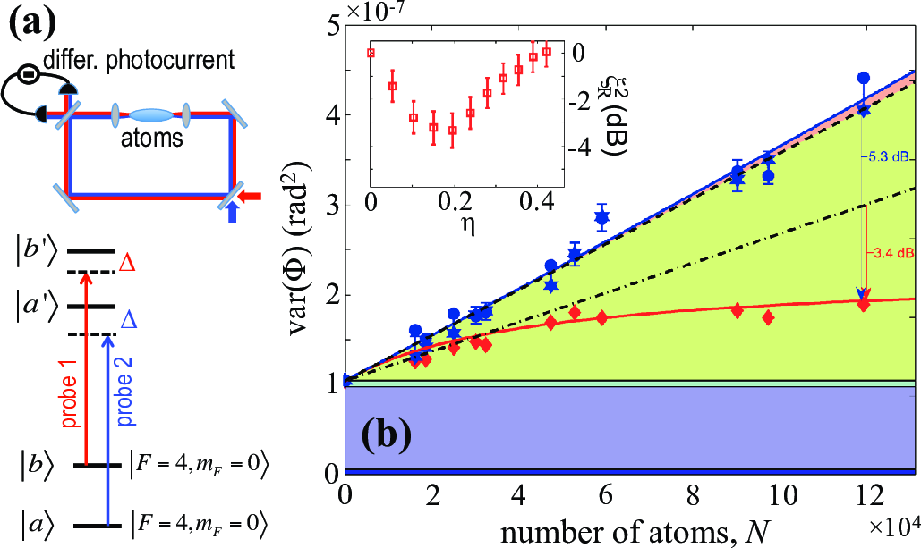
Appel et al. (2009) reported the first experimental demonstration of metrological spin squeezing (reaching ) via QND measurements in free space. This experiment used Cs atoms (with measured and optical depth ). Two equally intense and linearly polarized laser beams of different frequencies enter the arms of an optical Mach-Zehnder interferometer, see Fig. 27(a). The beams off-resonantly probe different atomic transitions and experience phase shifts proportional to the number of atoms in the probed levels Saffman et al. (2009). The detection of the relative phase shift accumulated in the optical path performs a QND measurement of the relative population in the two atomic levels Kuzmich et al. (1998); Saffman et al. (2009). Spin squeezing is quantified by correlations between two consecutive QND measurements. One finds , where and refer to the first and second phase shift detection, respectively, and the covariance expresses the correlations between the two measurements. The results reveal a spin squeezing dB, see Fig. 27(b). Furthermore, Louchet-Chauvet et al. (2010) have used a similar apparatus to perform a Ramsey sequence (between the two QND measurements) and demonstrated an atomic clock with a measured phase sensitivity 1.1 dB below the standard quantum limit.
Spin squeezing has also been experimentally performed by measuring the polarization rotation of probe light passing through a cloud of atoms. This technique was pioneered by Kuzmich et al. (1999, 2000), and more recently investigated in ensembles of spin-1/2 171Yb Takano et al. (2009, 2010); Inoue et al. (2013) and spin-1 87Rb atoms Sewell et al. (2012, 2013, 2014). In Sewell et al. (2012, 2014) spin squeezing was achieved using a two-polarization probing technique Koschorreck et al. (2010a, b). These experiments demonstrated dB Sewell et al. (2014) [ dB inferred Sewell et al. (2012)] using atoms, mainly limited by the photon shot noise of the readout light. Polarization-based QND measurements find direct application in entanglement-assisted optical magnetometry, see Sec. VII.3.
Puentes et al. (2013) have proposed to generate planar spin squeezing (see II.3.8) in spin-1 atomic ensembles via sequential QND measurements of two orthogonal spin components. Measurements by Colangelo et al. (2017b, a) in cold 87Rb atoms show phase and amplitude squeezing simultaneously, as well as entanglement between the atoms’ spins Vitagliano et al. (2018).
V.1.2 Cavity-based quantum nondemolition measurements in the dispersive regime
The strength of the interaction between the light and the individual atoms is usually weak, but can be enhanced by placing the atoms inside an optical cavity. This method is very promising as the squeezing factor increases with the cavity finesse, which can be pushed to large values. Moreover, a small single-pass optical depth is advantageous for applications in atomic clocks, since it allows to reduce atomic-density-dependent atom losses, dephasing, and systematic errors.
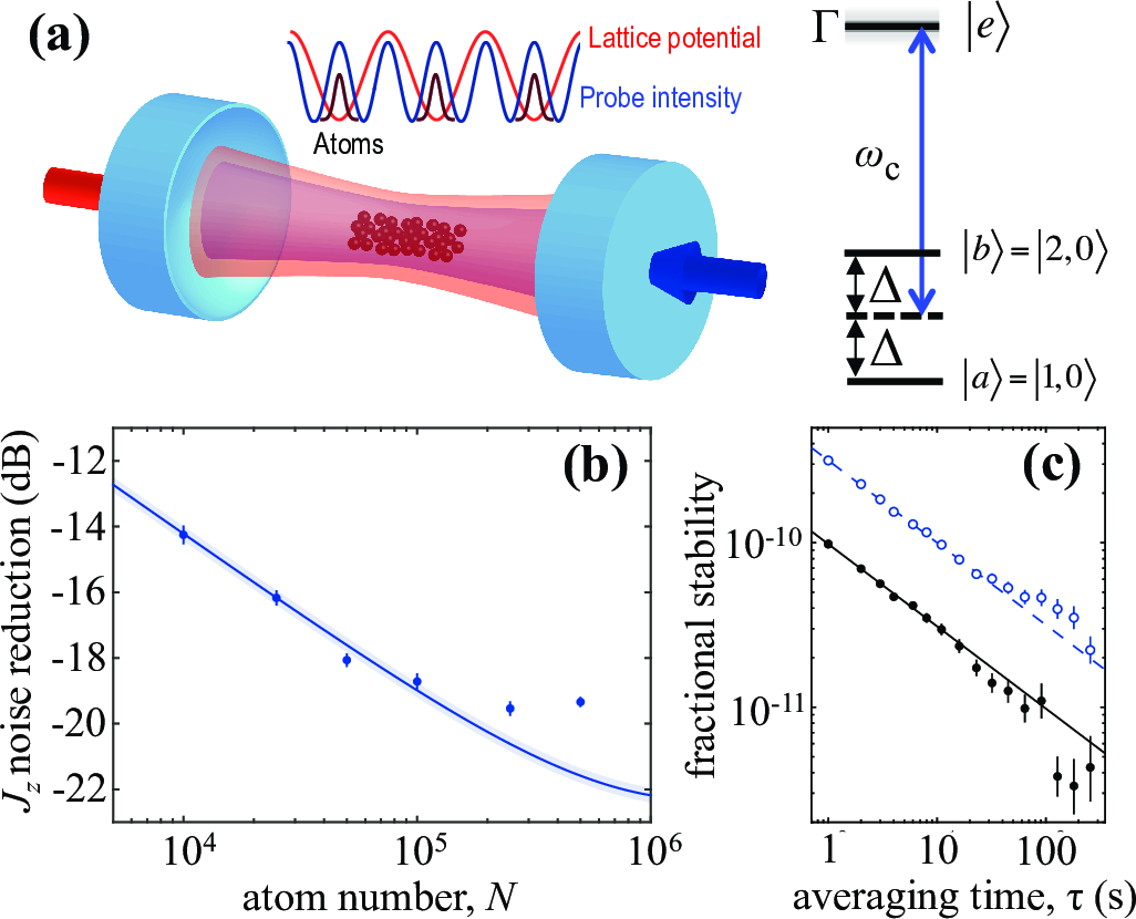
The essential features of dispersive atom-light interaction in a cavity Vernac et al. (2000); Nielsen and Mølmer (2008); Bouchoule and Mølmer (2002a); Madsen and Mølmer (2004) are captured by a simplified model comprising three-levels atoms, see Fig. 28(a). Each atom has two hyperfine levels and of energy difference , and an excited state with linewidth (spontaneous decay rate into free space). The atoms are placed in an optical cavity with resonance frequency and linewidth , driven resonantly with a single-atom-single-photon effective intra-cavity Rabi frequency . The detuning of the cavity from the and transitions is chosen of equal magnitude . Assuming homogeneous interaction (see Sec. II.5.3), low intra-cavity photon number (), and large detuning (), the coupling Hamiltonian is Schleier-Smith et al. (2010a)
| (96) |
where and are cavity mode operators. The effect of the light on the atoms is an ac Stark shift of the transition frequency between and . Atoms in () increase (decrease) the index of refraction seen by the probe light, so that the net effect is a shift of the cavity resonance by , where and are the numbers of atoms in and , respectively. This shift can be probed by injecting a laser into the cavity, providing a QND measurement of . A detailed analysis including decoherence associated with free-space scattering of the probe light shows the possibility to achieve Chen et al. (2014); Hosten et al. (2016a)
| (97) |
where is the single-atom cavity cooperativity. is the ratio between the number of photons scattered into the cavity mode and those scattered into free space, and quantifies the optical depth of an atom with respect to the cavity mode Tanji-Suzuki et al. (2011). Note that depends on the cavity geometry and is proportional to the cavity finesse Tanji-Suzuki et al. (2011).
Spin squeezing via cavity-based QND measurement has been first demonstrated by Schleier-Smith et al. (2010b) using magnetically-insensitive clock states of 87Rb atoms. This experiment reached a spin squeezing dB with respect to , referring to uncorrelated atoms ( accounts for spatial variation in the atom-light coupling due to the trapping lattice being incommensurate with the cavity mode used for probing, and ). This result is mainly limited by inhomogeneous dephasing due to the cavity locking light. Hosten et al. (2016a) have used a cavity of higher cooperativity and exploited probing and trapping beams of commensurate frequencies, achieving a uniform atom-light coupling, see Fig. 28(a). This avoids the need for spin-echo techniques required for non-uniformly coupled systems. This experiment demonstrated dB of improved phase sensitivity with respect to , with 87Rb atoms, and a spin squeezing dB, see Fig. 28(b). This represents the highest value in expected metrological spin squeezing and measured phase sensitivity gain to date.
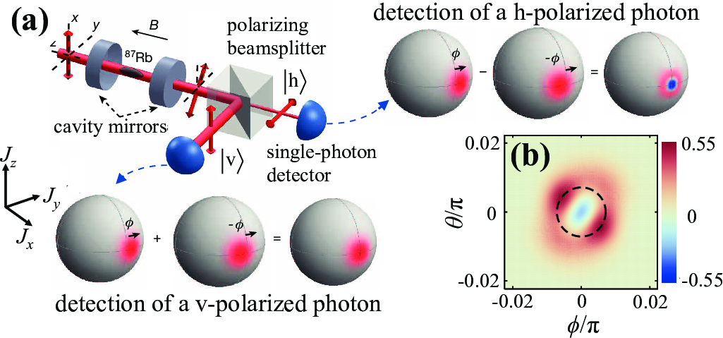
V.1.3 Heralded atomic entanglement created by single photon detection
In the preceding sections we have discussed the interaction of an atomic ensemble with an intense laser pulse ( photons in typical experiments), which is subsequently detected by a standard linear photodetector that does not resolve individual photons. The light in these experiments is effectively a continuous-variable quantum system. A different approach uses weak laser pulses in combination with single-photon counting, in close analogy to the techniques developed for atomic ensemble-based quantum repeaters Duan et al. (2001); Sangouard et al. (2011). These techniques allow to create a range of highly nonclassical states of a large number of atoms in a heralded way, i.e., conditioned on the detection of a single photon. The interaction of a linearly polarized photon with the atoms according to Eq. (93) produces a weak Faraday rotation of the photon polarization. Denoting and the vertical and horizontal polarizations, respectively, an atom-light system initialized in [where is a coherent spin state, see Sec. II.3] evolves by the QND interaction (93) to the state McConnell et al. (2013)
| (98) |
where and is the phase accumulated during the interaction. The detection of a vertically polarized photon projects the atomic ensemble to , whereas the detection of a horizontally polarized photon prepares . The entanglement properties strongly depend on the phase , and the quantum Fisher information is (without loss of generality we assume here that and )
| (99) |
where the plus (minus) sign holds for the detection of a vertically (horizontally) polarized photon. To leading order in , we have and : for , the state is metrologically more useful than . In particular, for , the (rare) detection of a horizontally polarized photon heralds the generation of , which is the one-excitation Dicke state. For , we have in Eq. (99) and the two states give approximatively the same quantum Fisher information. At , we get the NOON state . In the realistic scenario , the detection of a sequence of photons conditionally prepares more and more entanglement. For instance, disregarding losses and decoherence, the detection of h-polarized photons prepares the NOON state when . Finally, Chen et al. (2015b) have generalized the above method showing the possibility to generate a broad class of entangled states of many atoms using single photons having a tailored frequency spectrum and time-resolved detection.
Experimentally, the use of single-photon counting for preparing entangled states of an atomic ensemble has been pioneered by Christensen et al. (2013, 2014). These experiments have shown the expected increase of spin fluctuations due to the single-photon detection. McConnell et al. (2015) have demonstrated the generation of entanglement in an atomic ensemble of laser-cooled 87Rb atoms prepared in an optical cavity and probed with an off-resonant weak pulse (of about 200 photons) of vertically polarized light, see Fig. 29. The accumulated phase is , where is the characteristic atom-photon interaction time. For the experiment of McConnell et al. (2015) we have . This experiment has investigated the entangled state produced by the detection of a horizontally polarized photon, while the detection of vertically polarized photons gives, for these experimental parameters, only a slight spin squeezing. From the tomographic reconstructed density matrix it is possible to obtain a Wigner distribution with negative areas, see Fig. 29, and an entanglement depth (not related to metrological usefulness) of 2900 atoms. This work demonstrates how the information carried by a single (or a few) photon(s) can create entanglement in a large atomic ensemble. In Hu et al. (2017) the same authors have re-analyzed these data to show that the generated atomic state violates classical physics even if no assumptions related to quantum mechanics are made. This conclusion Kot et al. (2012), similarly to Bell inequalities Brunner et al. (2014), observes that marginal probability distributions measured for non-commuting observables do not always come from a joint probability distribution identified with a classical state. As in Schmied et al. (2016) (see Fig. 17), Hu et al. (2017) show that classical physics is insufficient for describing mesoscopic entangled states of atoms.
V.1.4 Cavity-based quantum nondemolition measurements in the normal mode splitting regime
The experiments discussed in the previous sections operate in the dispersive regime, where the cavity is far detuned from atomic resonance. In this section, we discuss quantum state preparation schemes where the cavity is tuned near an atomic resonance with respect to the atomic transition , see Fig. 30(a). Let us assume that atoms in do not to interact with the cavity mode, the number of atoms in is , and the system is driven weakly so that the mean number of atoms in is small with respect to . We have that atoms in cause a splitting of the cavity resonance frequency Chen et al. (2014) that depends on :
| (100) |
where is the cavity detuning from the atomic transition , is the bare cavity frequency, and is the single-atom-single-photon coupling rate (uniform coupling is assumed). At , the appearance of two well-resolved resonances separated by is referred to as collective vacuum Rabi splitting. In the limit of collective strong coupling the normal modes of the coupled system are well resolved: a measurement of thus allows to determine .
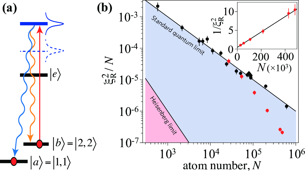
In the experiments of Bohnet et al. (2014); Chen et al. (2011); Cox et al. (2016), the atom number is measured non-destructively by probing the cavity resonant frequency with an additional probe laser injected into the cavity. The number of particles in level can be probed by first applying a resonant pulse between and and then repeating the QND measurement. A detailed analysis of the impact of decoherence in this system (mainly due to scattering of cavity photons into free space) can be found in Chen et al. (2014). In Chen et al. (2011) the optical cavity is tuned to resonance, , with . Chen et al. (2011) reported a spin squeezing dB ( dB inferred) relative to the standard quantum limit using 87Rb atoms ( is an effective atom number taking into account inhomogeneous coupling in the cavity, see Sec. II.5.3). In Bohnet et al. (2014); Cox et al. (2016) noise effects were considerably reduced taking advantage of a cycling transition Chen et al. (2014); Saffman et al. (2009), and higher collective cooperativity was reached. Experimental results demonstrate dB Bohnet et al. (2014), see Fig. 30, and dB Cox et al. (2016), using 87Rb atoms. The achieved spin squeezing witnesses the presence of useful particle entanglement Cox et al. (2016). This squeezing technique has been further combined with quantum feedback, reaching dB of deterministic spin squeezing Cox et al. (2016).
Resonant atom-light coupling in an optical cavity also offers the possibility to create entangled states beyond spin squeezing. Haas et al. (2014) have used an atom chip integrated with a high-finesse fiber-optical cavity in the strong-coupling regime Volz et al. (2011) to prepare a generalized state Dür et al. (2000) of cold 87Rb atoms. In this experiment the cavity and probe laser tuned on resonance with the transition. The single-atom strong coupling guarantees that the cavity only transmits light if all atoms are in level : a single atom in is sufficient to block the cavity transmission. The experiment of Haas et al. (2014) starts with all atoms in level , and a weak microwave pulse coupling and prepares the state , where to avoid multi-particle excitations. The cavity transmission is then measured with a probe-light beam. A low transmission heralds the QND preparation of the W state . The resulting state is characterized by state tomography, from which it is possible to extract a lower bound on the entanglement depth of atoms, at least.

V.1.5 Quantum state preparation via quantum Zeno dynamics
Quantum Zeno dynamics combines the coherent evolution of a system with the measurement of an initially unoccupied quantum state Facchi and Pascazio (2008): if the measurement is performed with high enough frequency, the measured state remains unoccupied. This profoundly modifies the system dynamics and allows engineering specific entangled states. In Barontini et al. (2015) a cavity-based measurement in the regime Volz et al. (2011) is used to prepare a generalized state of 36 87Rb atoms via quantum Zeno dynamics. The atoms are all initialized in level and coupled to the level by a microwave drive at Rabi frequency . The cavity is in resonance with the transition and transmits only if there are no atoms in level . The cavity transmission is probed at a rate much larger than . When no measurement is performed, the microwave Rabi coupling prepares the state after a time . In presence of the cavity measurement, the quantum Zeno effect forbids the preparation of and deterministically prepares the W state , see Fig. 31. From the density matrix extracted via state tomography, it is possible to obtain the quantum Fisher information. Values up to are reported by Barontini et al. (2015).
V.2 Light-mediated coherent interaction between distant atoms
In contrast to the measurement-based scheme of Sec. V.1, off-resonant atom-light coupling can also be used to realize a light-mediated coherent interaction between distant atoms. When the Stokes operator in Eq. (93) is proportional to , the Hamiltonian reduces to Agarwal et al. (1997); Zhang et al. (2003), corresponding to an effective one-axis twisting nonlinearity that generates unconditional spin squeezing Kitagawa and Ueda (1993). The condition can be realized in an optical cavity, see below. As a main difference with respect to contact interaction discussed in Sec. III.2, this light-mediated interaction can be applied to a dilute atomic sample, which is preferred for minimizing systematic errors in precision measurements. Moreover, in contrast to spin squeezing obtained from QND measurements, it deterministically produces known entangled states, independently from the detector performance. Furthermore, atom-cavity coupling can be easily switched on and off.

There are different proposals for the realization of an effective interaction between distant atoms. Takeuchi et al. (2005) have studied a double-pass Faraday interaction in free space where a polarized light beam passes twice through an atomic ensemble (after the first passage the polarization is properly rotated such that at the second passage). An improved version of this proposal has been discussed by Trail et al. (2010) using a quantum eraser to remove residual spin-probe entanglement. Schleier-Smith et al. (2010a); Zhang et al. (2015) have proposed the realization of light-induced atom-atom interaction in an optical cavity (also called cavity squeezing or cavity feedback). This relies on the dispersive interaction between one mode of the cavity and an ensemble of three-level atoms. As shown by Eq. (96) the atoms modify the cavity resonance frequency by an amount proportional to . When the cavity is driven by a probe laser of frequency tuned to the slope of the cavity resonance (), the intracavity photon number in Eq. (96), being detuning-dependent, changes linearly with the index of refraction of the atomic cloud (which, in turn, is proportional to ), see Fig. 32(b). Notice that tracing out the light field (which carries information about the atomic spin) yields a dissipative dynamics that limits the attainable squeezing Leroux et al. (2012). Pawłowski et al. (2016) analyzed the spin squeezing attainable with the cavity feedback method in presence of cavity losses and spontaneous emission, finding that in the limit . Finally, an alternative proposal to realize an effective one-axis twisting atomic Hamiltonian uses a four-wave Raman scheme to directly drive the atomic ensemble, where atoms communicate with one another by exchanging photons via a weakly-occupied cavity mode Sørensen (2002).
One axis twisting by light-mediated coherent interaction has been experimentally implemented in an optical cavity Leroux et al. (2010a, b), using an effective number of 87Rb atoms. The experiment implements the scheme of Schleier-Smith et al. (2010a). The squeezed state is characterized via spin-noise tomography and the contrast of Rabi oscillations. The results of Leroux et al. (2010a) are summarized in Fig. 32(c) and demonstrate a gain dB over ( dB over the sensitivity experimentally reached in absence of entanglement). Leroux et al. (2010b) have used the squeezed states generated with this method to realize an atomic clock with sensitivity dB below the standard quantum limit, see Sec. VII.
V.3 Quantum state transfer from non-classical light to atoms
Spin-squeezed states can be created via atom-light interaction by transferring quadrature squeezing of light to atomic spin squeezing Agarwal and Puri (1990); Kuzmich et al. (1997); Hammerer et al. (2010). This effect can be understood from the Jaynes-Cummings model Hamiltonian
| (101) |
describing the interaction of nondecaying two-level atoms with a light mode. Here and are the light creation and annihilation operators, respectively, are spin rising and lowering operators, see Sec. II.1, and is a coupling constant. The Heisenberg equations of motion for and can be found analytically within a frozen-spin approximation, assuming constant and equal to . We obtain Wineland et al. (1992, 1994)
| (102a) | ||||
| (102b) | ||||
where , , , and . Similar expressions can be obtained relating with , where . These equations predict that atomic spin squeezing can be achieved by first squeezing the light field, , and then transferring this quadrature squeezing onto the spins. Optimal spin squeezing is reached at . For strong squeezing the contrast decreases, and the frozen-spin approximation breaks down. Since the squeezed light is the source of spin squeezing in this method, the degree of squeezing is determined by the quality of the quadrature squeezed light.
Quantum state transfer from light to atoms has been first experimentally demonstrated by Hald et al. (1999) using a cloud of cold Cs atoms, following the theoretical proposal of Kuzmich et al. (1997). This experiment used a V-level scheme consisting of three atomic hyperfine levels Hald et al. (1999, 2000). The reduction of atomic spin noise below the projection noise of uncorrelated atoms is generated by the absorption of polarized coherent and squeezed vacuum light with opposite circular polarizations. The atomic fluctuations are read out by the differential photocurrent of a probe beam at the output ports of a polarizing beam splitter.
An alternative approach, mapping a quantum state of light onto an atomic state via electromagnetically induced transparency has been proposed by Fleischhauer and Lukin (2000), see also Phillips et al. (2001); Liu et al. (2001). Further studies include the mapping quantum states of light into a Bose-Einstein condensate with application to atom interferometers Szigeti et al. (2014) and atom lasers Fleischhauer and Gong (2002); Haine and Hope (2005).
VI Entangled states of trapped ions
Ensembles of trapped ions confined in electromagnetic traps and manipulated with laser beams are one of the most successful systems to generate and exploit entanglement Blatt and Wineland (2008); Wineland (2013). Direct applications include quantum information and computation Häffner et al. (2008); Roos (2014), quantum networks Duan and Monroe (2010), quantum simulations Blatt and Roos (2012); Schneider et al. (2012); Martinez et al. (2016) and, as reviewed here, quantum metrology. Trapped ions are well isolated from the environment, can be coherently manipulated, individually addressed and detected with almost unit efficiency Leibfried et al. (2003a).
Typical experiments Leibfried et al. (2003a) confine ions in a linear Paul trap [Fig. 33(a)], surface-electrode Paul trap Sterling et al. (2014); Mielenz et al. (2016), or Penning trap [Fig. 33(b)], followed by ground-state cooling. So far, up to 20 ions have been entangled in a Paul trap Monz et al. (2011) and up to about 200 ions in a Penning trap Britton et al. (2012); Bohnet et al. (2016). One- and two-dimensional ion arrangements are well suited for individually controlling and reading out internal states of the ions. We note that individual particle manipulation and detection are crucial for many quantum-computation and quantum-information tasks, but they are not necessary for quantum-enhanced metrology. Interesting metrological experiments can thus be also performed in Penning traps (where local manipulation is currently not available), which are well suited to store, manipulate, and entangle large numbers of ions.
In trapped-ion experiments, the qubit is formed by two internal (usually hyperfine) states and of each ion. This internal qubit can be coupled by an electromagnetic field to external (motional, vibrational) degrees of freedom, see Fig. 33(c). A key aspect is the local detection of the internal ion’s state with extremely high efficiency. This is usually achieved by resonant fluorescence. Detection errors arise if the qubit changes its state during the detection interval or if photons scattered off trap electrodes are mistaken for fluorescence photons. In Myerson et al. (2008); Harty et al. (2014) qubit detection errors smaller than are reported.
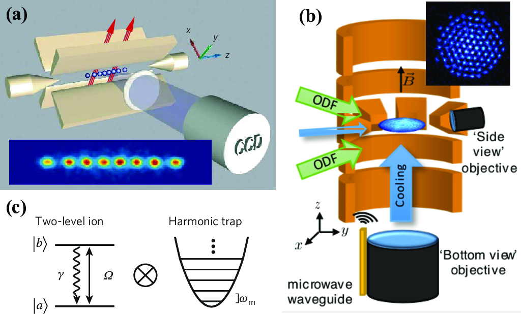
VI.1 Generation of metrologically useful entangled states of many ions
The generation of entanglement between different qubits is one major challenge in quantum information processing with trapped ions Wineland et al. (1998). The Coulomb force pushes the ions apart to a distance much larger than the Bohr radius and thus prevents state-dependent ion-ion interactions in absence of external electromagnetic fields. However, as a consequence of the Coulomb force, the normal modes of motion in the trap are shared among all ions and can provide a means for entangling the qubits. Most of the schemes for entangling trapped ion qubits are based on internal-state-dependent forces acting on the ions, generated by external electromagnetic fields. These forces can be arranged in time and frequency in such a way that an effective entangling operation is carried out between two or more qubits and no entanglement persists between the qubits and the vibrational degrees of freedom.
The entangling gates can be broadly classified in three categories, according to the way the electromagnetic fields interact with the ions: i) Quantum gates induced by a laser beam that interacts with a single ion at a time as originally proposed by Cirac and Zoller (1995). The ion is entangled with a vibrational mode of the ion string and the entanglement is subsequently transferred from the vibrational mode to the internal state of a second ion. ii) Quantum gates induced by an electromagnetic field that simultaneously addresses two or more ions, either through optical ac Stark shifts Leibfried et al. (2003b); García-Ripoll et al. (2005); Kim et al. (2010); Sørensen and Mølmer (2000); Milburn et al. (2000); Lee et al. (2005); Kim et al. (2009); Mølmer and Sørensen (1999); Solano et al. (1999); Sørensen and Mølmer (1999), through static magnetic-field gradients in combination with homogeneous radio-frequency fields Mintert and Wunderlich (2001); Welzel et al. (2011); Johanning et al. (2009b, a), or with radio-frequency field gradients Ospelkaus et al. (2008, 2011). As an important advantage, these gates do not require to cool all ion normal modes to their ground states, but only the ion motion to be well within the Lamb-Dicke regime , where is the displacement of an ion along the laser propagation direction and the laser wavelength. The basic idea is to drive a phonon (normal) mode of frequency by a periodic state-dependent force with frequency . In the rotating-wave approximation, the Hamiltonian describing this conditional interaction is Roos (2014)
| (103) |
where is an operator acting on the (internal) qubit states, and are the harmonic oscillator creation and annihilation operators of the addressed normal mode, respectively, is a coupling strength, and . The propagator corresponding to this (time-dependent) Hamiltonian is
| (104) |
where and . If the interaction time is chosen such that , then the propagator reduces to . A vibrational mode becomes transiently entangled with the qubits before getting disentangled at the end of the gate operation, resulting in an effective nonlocal operation capable of entangling the ions. The conditional phase gate Leibfried et al. (2003b) is obtained by setting in Eq. (104), and is realized by placing the ions in a qubit-state-dependent potential created by two counter-propagating laser beams. The Mølmer-Sørensen gate Mølmer and Sørensen (1999); Sørensen and Mølmer (2000) is obtained setting (or ). This gate is realized by a bichromatic laser field tuned close to the upper and lower motional sideband of the qubit transition Benhelm et al. (2008); Sackett et al. (2000). In both gates, the propagator is of the kind , formally equivalent to Kitagawa-Ueda one-axis twisting, see Sec. III.2. Spin-dependent optical dipole forces generated by a pair of off-resonance laser beams with different frequencies, addressing many normal modes simultaneously, have been recently used to engineer tunable Ising spin-spin coupling Kim et al. (2009); Porras and Cirac (2006); Lee et al. (2005). The resulting propagator is Porras and Cirac (2006)
| (105) |
where , is the distance between the th and th ions and can be tuned by adjusting the laser frequencies in the range Britton et al. (2012); Schmied et al. (2011). Ising spin-spin couplings have been implemented in a linear Paul trap with up to 20 ions Islam et al. (2013); Jurcevic et al. (2014); Richerme et al. (2014) and in a Penning trap forming a 2D Coulomb crystal of 200 ions Britton et al. (2012); Bohnet et al. (2016), see Fig. 33(b). iii) A third way to generate ion entanglement is based on performing joint measurements on photons that are first entangled with ion qubits Moehring et al. (2007); Stute et al. (2012); Casabone et al. (2013). This scheme enables the generation of entanglement between ions separated by large distances and does not require the ions to be in the Lamb-Dicke regime.
VI.2 Quantum metrology with trapped ions
VI.2.1 Quantum metrology with two ions
The first deterministic generation of entanglement of two trapped ions was reported by Turchette et al. (1998). This experiment was readily followed by the demonstration of a phase sensitivity below the standard quantum limit Sackett et al. (2000); Meyer et al. (2001). Meyer et al. (2001) reported the creation of the state
| (106) |
of two 9Be+ ions via a Mølmer-Sørensen gate in a linear Paul trap. Here is a tunable parameter proportional to the laser pulse duration. The state (106) is spin-squeezed, for . It reaches the Heisenberg limit at , corresponding to the creation of a maximally entangled state. However, at , and any technical noise prevents detecting the maximally entangled state as spin squeezed. The experiment of Meyer et al. (2001) reached at the experimentally optimal working point . A phase estimation with sensitivity below with the maximally entangled state () was demonstrated by applying a spin rotation followed by . Measuring the parity led to a sensitivity , where . Many experiments with two ions have have reported parity oscillations from which it is possible to extract the phase sensitivity Leibfried et al. (2003b): in particular, in magnetic-field-insensitive clock states of 111Cd+ Haljan et al. (2005), and using an optical transition in 40Ca+ Home et al. (2006); Noguchi et al. (2012); Monz et al. (2011) and 88Sr+ Navon et al. (2014) ions. A very high visibility of the parity signal has been reported with 40Ca+ Benhelm et al. (2008) and 43Ca+ Ballance et al. (2016) ions, see also Gaebler et al. (2016) for the high-fidelity generation of the two-qubit GHZ states with 9Be+ ions. Finally, Meyer et al. (2001) also reported a full Ramsey sequence, where the maximally entangled state is generated between two Ramsey pulses and the phase is proportional to the interrogation time. In this case, the initial probe state is a symmetric Dicke (or twin-Fock) state. By measuring the parity, it was possible to reach a spectroscopic sensitivity . Noguchi et al. (2012) reported the creation of symmetric Dicke states of two and four 40Ca+ ions.


VI.2.2 Quantum metrology with GHZ states of several ions
The maximally entangled (or “Schrödinger cat”) state
| (107) |
has been created with up to 9Be+ ions Leibfried et al. (2005) and 40Ca+ ions Monz et al. (2011) in a linear Paul trap. This state is formally obtained from , where , see Sec. III.2. When applying a spin rotation , the state (107) transforms as , such that the relative phase between and is . The state can be detected after a Rabi rotation around the -axis. The probability to obtain atoms in level and atoms in level is . These probabilities oscillate with a frequency times faster than that of a single qubit. Therefore, most observable properties of these states, such as the occurrence of atoms in level or , or collective properties such as the parity of the relative number of particles in the output state Bollinger et al. (1996), feature this rapid oscillation. Notably, applying the nonlinear transformation again after phase encoding, one obtains only two detection events ( atoms in level or ) that can be experimentally distinguished with high efficiency Leibfried et al. (2004, 2005). Experiments exploring quantum metrology with states (107) generally report dichotomic events—the parity of the relative atom number, in Leibfried et al. (2004); Monz et al. (2011), or the detection of all atoms in the same level in Leibfried et al. (2004, 2005). Figure 34(a) shows an example of parity oscillations, , where the visibility accounts for experimental noise and imperfect state preparation. The corresponding the Fisher information, , is
| (108) |
It reaches the maximum value when . It is thus possible to detected useful entanglement and obtain sensitivities below the standard quantum limit when (corresponding to ). Metrologically-useful maximally entangled states are detected when [corresponding to , obtained from Eq. (33) with ]. Figure 34(b) gives an overview of the experimental results obtained with cat states of trapped ions. In Monz et al. (2011) the fringe visibility of parity oscillations was sufficiently high that the Fisher information witnesses metrologically useful genuine -particle entanglement up to ions Pezzè et al. (2016).
Note that the fast oscillations of the output probabilities obtained with the state (107) seem to prevent the unambiguous estimate of a phase larger than Berry et al. (2009); Pezzè and Smerzi (2007); Boto et al. (2000); Mitchell (2005). A phase estimation at the Heisenberg limit with no constraint on in can be obtained using states (107) with different numbers of particles. The optimal sequence provides (at ), where is the total number of particles used Pezzè and Smerzi (2007).
VI.2.3 Spin squeezing and useful entanglement of many ions
Recently, entanglement and metrological spin-squeezing of hundreds of trapped 9Be+ ions have been demonstrated in a Penning trap Bohnet et al. (2016). The experiment realized a homogeneous Ising spin-spin interaction Kitagawa and Ueda (1993) (i.e., in Eq. 105) corresponding to the one-axis twisting model, see Sec. III.2. Figure 35 shows , optimized over time, as a function of the number of ions ranging from to . For long interaction times, the state wraps around the Bloch sphere and spin squeezing is lost (see Sec. III.2). In this case, the experimental data of Bohnet et al. (2016) still show signaling useful entanglement, where the Fisher information has been extracted following the Hellinger method of Strobel et al. (2014). For an analysis of decoherence in this system see Foss-Feig et al. (2013).
VII Working entanglement-enhanced interferometers and prospects for applications
Atomic ensembles are routinely used as precision sensors of inertial forces or external fields, or as atomic clocks, which usually operate as Ramsey interferometers Wynands and Weyers (2005); Wynands (2009); Cronin et al. (2009); Kitching et al. (2011); Bordè (2002); Barrett et al. (2016). The accumulated phase is , where is the Ramsey interrogation time (not the overall measurement cycle time) and is the parameter to be estimated. In an atomic sensor, , where is the energy shift between the two interferometer modes, induced by an external field, an acceleration, a rotation, or a force. In an atomic clock, , where is the instantaneous frequency of a local oscillator to be locked to the transition frequency between the two atomic levels that define the clock. The standard quantum limit for the estimation of the frequency is, from Eq. (29),
| (109) |
where we have expressed the number of measurements in terms of the total averaging time and the cycle time of the experiment, with . Using separable states, if quantum noise dominates over technical noise and is optimized, the sensitivity can thus only be increased by increasing the interrogation time , the number of particles, and/or the total averaging time . In realistic setups this is not always possible: every sensor has an optimal working range for and , and drifts always limit the duration over which identical state preparation can be assumed Bak et al. (1987). In general, increasing the atom number leads to systematic errors due to collisions that spoil the sensitivity. Ramsey interrogation times are limited by mechanical restrictions (e.g., the limited ballistic flight time in fountain clocks), by the desired temporal resolution (e.g., when measuring high-frequency magnetic fields in broadband magnetometers), or decoherence (e.g., the phase coherence time of the local oscillator in atomic clocks). Can entangled states improve the performance of atomic sensors and, if so, under what conditions?
Entangled states are typically more susceptible to decoherence than separable states during phase encoding. Thus their gain (i.e., their more favorable scaling of phase sensitivity with ) is often counterbalanced by the requirement of shorter interrogation times Huelga et al. (1997). Whether or not an improvement is possible can only be decided after a detailed analysis of a specific sensor taking its actual limitations into account, and ultimately hinges on an experimental demonstration. As an example we note that squeezing of light has recently been used to improve the performance of a laser-interferometer gravitational wave observatory The LIGO Scientific Collaboration (2011); Aasi et al. (2013). The aim of this section is to review the state of the art of entanglement-enhanced measurements with atomic ensembles beyond proof-of-concept demonstrations, and to discuss prospects for applications.
VII.1 The influence of noise and decoherence
A common and central aspect of quantum-enhanced metrology is the fragility of useful entangled states when coupled to the environment. Noise affects the preparation of the probe state, phase encoding, and detection. The literature has focused mainly on specific noise models and only few general results are available. An important challenge is to devise protocols (e.g., differential schemes, or error correction), special phase sensing situations (e.g., non-Markovian, or transverse noise) and detection schemes that make metrology below the standard quantum limit robust against noise.
VII.1.1 General results
Phase encoding in the presence of noise can be formally described by a -dependent completely-positive trace-preserving map Rivas and Huelga (2012), such that , where and are the probe and output state, respectively. The evolution from to can be conveniently studied by introducing additional degrees of freedom that are not under control and play the role of an “environment”. The action of any quantum channel can be described via its Kraus representation , where are Kraus operators, is an orthonormal and complete set of states ( guarantees ), and is the initial state of the environment (taken pure, without loss of generality). We recall that a Krauss representation is not unique: we can generate a new set by a unitary (eventually -dependent) transformation Nielsen and Chuang (2000).
In the enlarged Hilbert space , given by the product of the Hilbert space of the system and of the environment, phase encoding is modeled by a unitary operation . Decoherence is taken into account by tracing over the environment: , where is a purification of and a purification of the probe state . We recall that two purifications and of the same state are related via unitary operations acting only on the environment space Nielsen and Chuang (2000), . Discarding part of the information regarding the unitary phase encoding in motivates the inequality
| (110) |
valid for all purifications of , where
| (111) |
Equation (110) suggests to search for the minimum of over all purifications of Escher et al. (2011, 2012). Following Uhlmann’s theorem Uhlmann (1976), Escher et al. (2011) have indeed shown that
| (112) |
see also Fujiwara and Imai (2008). In other words, there is always an environment that—when monitored together with the system—does not lead to more information about than monitoring the system alone. In particular, for an initial pure state , Eq. (112) can be rewritten as Escher et al. (2011)
| (113) |
where the mean values are calculated over and the minimization runs over all Kraus representations of the quantum channel. It is worth pointing out that, even if the optimal purification in Eq. (112), or the optimal set of Kraus operators in Eq. (113), are difficult to find, specific choices may yields non-trivial upper bounds to the quantum Fisher information Escher et al. (2011).
A special case of the above formalism is that of a -independent quantum channel where noise acts after phase encoding. In this case the quantum Fisher information never increases Petz (2002); Fujiwara (2001):
| (114) |
For example, the partial trace operation can only decrease the quantum Fisher information, consistent with the intuition that ignoring part of a system can only decrease the information about the estimated parameter. The equality in Eq. (114) is always obtained if is unitary, because unitary -independent transformations can be absorbed into a redefinition of the optimal measurement saturating the quantum Fisher information.
VII.1.2 Uncorrelated decoherence
A typical example of the fragility of frequency estimation with respect to noise has been discussed by Huelga et al. (1997). Let us consider a single atom prepared in the superposition that evolves freely for a time , according to the Hamiltonian , and acquires a phase in the presence of local Markovian dephasing. The probability to find the probe in its initial state is , where is the dephasing rate. If the phase estimation is repeated times in parallel (using a total of particles), a calculation of the Cramér-Rao bound gives at the optimal Ramsey time , with a total measurement time of . If we take a GHZ state in the presence of the same source of (single-particle) dephasing, the probability to find the probe in the initial state is : it oscillates times faster than in the single-particle case (this is typical for GHZ states, see Sec. II.3.7), but the visibility of these oscillations decays times quicker. A calculation of the Cramér-Rao bound gives , reached already at the optimal time . Repeating this experiment times in the same total measurement time (neglecting experimental dead-time, ) allows for a reduction of the measurement uncertainty to . In this example, the ideal sensitivity enhancement offered by GHZ states for disappears in the presence of arbitrarily small uncorrelated dephasing (). Although the overall absolute sensitivity is not improved, the GHZ state reaches the sensitivity limit with times faster with respect to the uncorrelated atoms: this may be of practical interest when experimental constraints require Huelga et al. (1997); Shaji and Caves (2007). An optimization over probe states shows that at most a constant factor of in the absolute frequency error can be gained in the presence of single-particle dephasing Huelga et al. (1997); Escher et al. (2011); Ulam-Orgikh and Kitagawa (2001).
Bounds to the quantum Fisher information in presence of more general uncorrelated decoherence have been discussed in the literature. Let us consider particles prepared in a state and a noisy channel that acts independently on each particle, such that . The maximum of the quantum Fisher information over all possible probe states is bounded as Fujiwara and Imai (2008)
| (115) |
where , , denotes the operator norm, and the minimization runs over all equivalent Kraus representations of the channel . In particular, if there exists a Kraus representation such that , then the second term in Eq. (115) vanishes and has—asymptotically in —a bound that scales linearly with . Relevant single-particle quantum channels fulfill the condition181818A notable class of channels that fulfill is that of quantum simulable channels Kołodyński and Demkowicz-Dobrzański (2013), i.e., those that can be written as , where is a -independent channel Matsumoto (2010). acts on an enlarged space including the auxiliary state that contain all information about the parameter. We have , that follows from Eq. (114) and the additivity of the quantum Fisher information. A quantum simulable channel may admit several decompositions, the optimal one being that giving the smallest value . When has a diagonal form, , where is some basis of the enlarged Hilbert space, the channels is said to be classical simulable Matsumoto (2010). In this case we have Demkowicz-Dobrzański et al. (2012), where can be found from the geometric properties of the convex space of quantum channels Bengtsson and Zyczkowski (2006). In particular, for channels that lie into the set of completely-positive trace-preserving maps away from its boundary, including full-rank channels. Demkowicz-Dobrzański et al. (2012); Kołodyński and Demkowicz-Dobrzański (2013); Escher et al. (2011). This means that, for those channels, the phase sensitivity achievable with an arbitrary probe state is , with . Therefore, asymptotically in the number of particles, the optimal achievable phase sensitivity has a scaling and the possible gain over the standard quantum limit is only limited to a prefactor (when ). We notice however that this is an asymptotic result for : entangled states may still provide a scaling of phase sensitivity better than the standard quantum limit, up to the Heisenberg limit, even for relatively large .
According to Eq. (115) a necessary condition to overcome the asymptotic scaling of precision is to have . It has been shown that this condition can be achieved for relatively short interrogation times in the case of non-Markovian noise Chin et al. (2012); Matsuzaki et al. (2011) and also when considering dephasing noise perpendicular to phase encoding evolution Chaves et al. (2013). In these cases, quantum-enhanced frequency estimation can be found in the limit . In particular, Chin et al. (2012); Matsuzaki et al. (2011) have shown that a frequency variance can be reached for an interrogation time under general models of non-Markovian phase noise; see also Macieszczak (2015); Berrada (2013); Szańkowski et al. (2014); Smirne et al. (2016). Moreover, Chaves et al. (2013) have shown that if Markovian dephasing is acting along a spin direction perpendicular to the phase encoding, in the limit a sensitivity can be obtained for interrogation times . The possibility to reach the Heisenberg limit in this case has been discussed by Kessler et al. (2014b); Dür et al. (2014) when making use of quantum error correction techniques (see below). The orientation-dependent lifetime of spin-squeezed states has been investigated experimentally by Leroux et al. (2010b).
VII.1.3 Correlated phase noise, differential interferometry, and decoherence-free subspaces
In many systems, a significant source of noise is correlated dephasing, where all atoms are subject to the same stochastic fluctuation of the phase shift. For instance, correlated dephasing is relevant in experiments with ions stored in linear Paul traps Monz et al. (2011); Roos et al. (2006): phase fluctuations are caused by noisy stray fields inducing random energy shifts of the atomic levels. Correlated phase noise is modeled as
| (116) |
where describes the phase fluctuations around and is the phase-encoding unitary tramsformation. The probability of a generic detection event is
| (117) |
where . Inserting into Eq. (7) allows to calculate the Cramér-Rao bound in presence of arbitrary phase noise. Taking for , , and considering states symmetric under particle exchange, we obtain
| (118) |
where is an eigenstate of with eigenvalue . As a consequence of correlated phase noise, off-diagonal elements are exponentially suppressed at a rate proportional to . Equation (118) predicts that the coherence of a -qubit GHZ state decays faster than that of a single qubit by a factor . This effect, also known as super-decoherence, has been demonstrated experimentally with maximally entangled states of 40Ca+ ions by adding a variable delay time between creation and coherence investigation Monz et al. (2011). Correlated phase noise is more dramatic than uncorrelated dephasing discussed above. Indeed, taking the sum of (the smallest possible) quantum and phase noise [see also Escher et al. (2012); Genoni et al. (2011)], we have
| (119) |
which does not scale with for , in contrast with uncorrelated dephasing where .
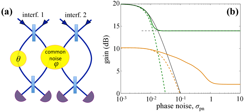
Correlated phase noise can be counteracted by a differential interferometer scheme Landini et al. (2014), see Fig. 36(a), that consists of two interferometers running in parallel. The phase shift in the first interferometer is , while that in the second interferometer is , where is the signal phase to be estimated and are shot-to-shot random phases. Taking a Gaussian as above, and perfectly correlated interferometers with , we have
| (120) |
where and are eigenstates of with eigenvalues . Components with are insensitive to phase noise and define a decoherence-free subspace Zanardi and Rasetti (1997); Lidar et al. (1998). This condition is met by nontrivial states achieving the Heisenberg limit of phase sensitivity Dorner (2012); Landini et al. (2014); Jeske et al. (2014). Figure 36(b) illustrates examples showing the superior performance of a differential scheme (thick solid lines) with respect to a single interferometer (dashed lines) affected by the phase noise with the same amplitude . For a differential scheme where each interferometer is fed with NOON states and relative particle number measurement, the Fisher information saturates to for Landini et al. (2014). Finally, noise correlations between the two interferometers are crucial: achieving the Heisenberg limit in a differential interferometer requires Landini et al. (2014). Roos et al. (2006) demonstrated experimentally the preparation of a designed entangled state of two ion qubits in a decoherence-free subspace and proved its robustness by measuring the electric field quadrupole shift while removing sensitivity to a noisy magnetic field environment. In Monz et al. (2011) decoherence-free states with up to 8 ions were constructed, achieving coherence times of 100, see also Pruttivarasin et al. (2015). In specific cases, entanglement can be preserved in the presence of correlated dephasing even if the state is not in a decoherence-free subspace Carnio et al. (2015).
VII.1.4 Error correction
Quantum error correction techniques are crucial in quantum computing Nielsen and Chuang (2000); Shor (1995); Steane (1996) and can be used to counteract the effect of noise in quantum metrology Kessler et al. (2014b); Dür et al. (2014); Arrad et al. (2014); Ozeri (2013); Plenio and Huelga (2016); Herrera-Martí et al. (2015). These schemes correct the imprinting of phase information in a quantum state against decoherence by employing ancilla qubits that neither interact with the parameter nor are subject to noise. Noise operators map the state to ancilla Hilbert subspaces orthogonal to the phase encoding subspace. Error correction is accomplished by projective measurements into the orthogonal subspaces, and then applying a correction sequence. These techniques can be used to extend the coherence time and/or to achieve the Heisenberg limit for certain noise models Kessler et al. (2014b); Dür et al. (2014); Arrad et al. (2014); Ozeri (2013). Lu et al. (2015) have provided conditions under which the quantum Fisher information, rather than the full quantum state, can be protected under a class of noisy channels.
VII.1.5 Particle losses
The incoherent loss of particles can strongly impact the usefulness of a state for quantum metrology. A paradigmatic example is the NOON state: the loss of a single particle transforms Eq. (43) into the incoherent mixture , which is useless for phase sensing. Losses can be modeled by a beam splitter of transmission coefficient that equally couples each interferometer arms to environment modes. This leads to the bound of sensitivity
| (121) |
that is valid for any probe state Escher et al. (2011): when , is bounded by the Heisenberg limit, while for one obtain . In this case, one recovers the scaling with at best, a prefactor that is for .
For ultracold atoms, collisional losses are especially relevant. One-body losses are due to collisions of trapped atoms with residual hot atoms due to imperfect vacuum, whereas two- and three-body losses are caused by inelastic collisions within the trapped cloud and are relevant in dense samples. In particular, Li et al. (2008a) have studied the impact of atom losses during the preparation of spin-squeezed states via one-axis twisting (see Sec. III.2) and have shown that for one-body losses, assuming and an optimal evolution time. For two-body losses, the optimal does not depend on , while for three-body losses and there is a finite optimal number of particles for squeezing.
VII.1.6 Finite detection efficiency
Low efficiency in the detection of large atom numbers is one of the main limitations in many current quantum-enhanced metrology experiments. Finite detection efficiency blurs the interferometer signal and thus degrades its phase sensitivity. A noisy detector can be modeled as a beam splitter of transmission coefficient followed a perfect detector. In this case (assuming equal efficiency for both detectors), the bound (121) applies. More generally, we can model an imperfect detection by replacing ideal probabilities —here is the result of a measurement (we restrict for simplicity to projective measurements but the discussion can be straightforwardly extended to generalized measurements, see footnote 2)—with
| (122) |
where is a convolution function giving the probability to obtain the result when the “true” value is . In practice, one can use a normalized Gaussian , where accounts for the detection noise (independent on the detection signal, for simplicity) and for the attenuation of the signal. Finite detection efficiency limits the distinguishability of the probability distribution when changing the parameter and thus decreases the Fisher information, see Sec. II.2.4.

An interaction-based readout can make phase estimation robust against detection noise, removing the requirement of single-atom resolution to reach a precision approaching the Heisenberg limit Davis et al. (2016); Fröwis et al. (2016); Nolan et al. (2017); Anders et al. (2018). In an interaction-based readout, some nonlinear unitary evolution (e.g., generated by the interaction between the particles) is applied before the readout measurement, such that the probability of a result is given by . For instance, can be the inverse of the nonlinear transformation that generates the entangled probe state, thus realizing an echo sequence Macrì et al. (2016); Garttner et al. (2017). Notice that SU(1,1) interferometers, see Sec. IV.3.4, take advantage of an interaction-based readout and their robustness to detection noise has been emphasized by Marino et al. (2012); Ou (2012). An example of the advantage offered by the interaction-based readout is illustrated in Fig. 37(a). This effect can be understood as a phase magnification Hosten et al. (2016b): output probability distributions of phase-shifted states become more distinguishable (and thus less prone to detection noise) when applying a nonlinear evolution prior to readout. As a simple example, following Leibfried et al. (2005), let us consider phase estimation using the NOON state (43). Applying a phase encoding followed by a Rabi rotation around the -axis, one can measure the relative number of particles in and . The phase information is included in fine structure of this probability distribution. These structures are washed out by the detection noise of just one atom, see Fig. 37(b). However, applying the transformation after phase encoding (i.e., to ) one obtains . Only two detection events are possible ( atoms in or ) that can be experimentally distinguished even for a large detection noise (e.g., ), see Sec. 37(c).
A nonlinear readout has been exploited by Leibfried et al. (2004, 2005) for quantum-enhanced metrology with GHZ states of trapped ions (see Sec. VI.2), and more recently, by Linnemann et al. (2016) for the realization of a SU(1,1) interferometer with a spinor Bose-Einstein condensate (See Sec. IV.3.4). In the experiment of Hosten et al. (2016b) the collective spin of 87Rb atoms is first squeezed via a light-mediated interaction in an optical cavity (see Sec. V.2), and then rotated by an angle . After a second period of collective spin interactions in the cavity, the state is detected via fluorescence imaging, demonstrating a phase sensitivity 8 dB below the standard quantum limit, using a detection with a technical noise floor 10 dB above the projection noise of uncorrelated atoms.
VII.2 Atomic clocks
Passive atomic clocks operate by locking—via a feedback loop—the frequency of a local oscillator to the transition frequency between two levels and of an atom Wynands and Weyers (2005); Wynands (2009); Ludlow et al. (2015); Kohlhaas et al. (2015). The standard clock configuration is based on Ramsey spectroscopy Ramsey (1963). Atoms are initially prepared in the clock state . A near-resonant pulse from the local oscillator prepares a superposition of and . Finally, after a time of free evolution (Ramsey interrogation time), a second pulse is applied to the atoms. The difference is estimated from a measurement of the atom number in the two levels and used for a feedback loop that steers the toward . Atomic clocks are characterized by their accuracy and stability Vanier and Audoin (1992). Accuracy refers to the frequency offset from the ideal value, whereas stability describes the fluctuations of the instantaneous frequency from . Improving the stability of time-keeping is one of the primary targets of quantum-enhanced metrology. It also allows for faster evaluation of systematic errors, which in turn can improve the accuracy Nicholson et al. (2015).
The standard figure of merit for quantifying the stability of a clock is the Allan standard deviation of the relative frequency fluctuations Vanier and Audoin (1992),
| (123) |
where is the relative change of the clock frequency between two successive averaging bins of duration . The Allan deviation quantifies the discrepancy between two consecutive observations of the clock frequency averaged for a time , including dead times in preparation of the sample and data acquisition. For an atomic clock operating at the standard quantum limit with uncorrelated (shot-to-shot) measurements, we have
| (124) |
where is the clock cycle duration ( being the number of measurements performed in a time ). Currently, the stability of atomic clocks is nearly Nicholson et al. (2012); Hinkley et al. (2013); Bloom et al. (2014) or already—as in the case of ion spectroscopy Itano et al. (1993) and fountain clocks Santarelli et al. (1999)—limited by Eq. (124). In principle, the clock stability is optimized by extending the interrogation time until atomic decoherence dominates in the interferometer output signal. In practice, a main limitations of current clocks—in particular of optical clocks using trapped atoms—are random fluctuations of the local oscillator frequency. These limit the stability of frequency comparisons to interrogation times of the order of a second, well short of the limits imposed by atomic decoherence, such as excited-state decay Wineland et al. (1998).
Theoretical studies of entanglement-enhanced atomic clocks have focused on the impact of collective dephasing caused by fluctuations of the local oscillator frequency, taking into account temporal noise correlations as well as the feedback mechanism that controls the local oscillator frequency. State and measurement optimization Bužek et al. (1999); André et al. (2004); Rosenband (2011) as well as adaptive schemes Kessler et al. (2014a); Borregaard and Sørensen (2013) have been considered. André et al. (2004) have shown the possibility of achieving an entanglement-enhanced stability by optimizing over a family of moderately squeezed states. More recently, Borregaard and Sørensen (2013) have shown that using squeezed states and weak output measurements it is possible to achieve , thus reaching the Heisenberg scaling. The adaptive optimization of probe state and output measurement has been studied for low atom number by Rosenband (2011) and Mullan and Knill (2014). The adaptive use of GHZ states in an atomic clock—in the presence of local oscillator noise only—has been considered in Kessler et al. (2014a), see also Leroux et al. (2017). Overall, these protocols show that entangled states can be can useful to track and stabilize the fluctuations of the local oscillator over long time scales. Finally, quantum bounds of frequency stability have been discussed by Chabuda et al. (2016); Fraas (2016).
VII.2.1 Entanglement-assisted atomic clocks
Atomic clocks with a performance beating the standard quantum limit have been experimentally demonstrated with two trapped ions Meyer et al. (2001), ensembles of cold thermal atoms Louchet-Chauvet et al. (2010); Leroux et al. (2010b); Hosten et al. (2016a) and Bose-Einstein condensates Gross et al. (2010); Kruse et al. (2016); Ockeloen et al. (2013). The neutral atom experiments have realized microwave-frequency clocks on magnetic field-insensitive hyperfine transitions with spin-squeezed states as input.191919Note that, to date, squeezing has not yet been realized on an optical transition. Monz et al. (2011) have created GHZ states on the optical clock transition of 40Ca+ ions. Leroux et al. (2010b) measured an Allan deviation of for their squeezed clock, corresponding to an improvement of 4.5 dB in variance beyond the standard quantum limit, see Fig. 38. More recently, Hosten et al. (2016a) performed a similar measurement, reaching , or 10.5 dB in variance beyond the standard quantum limit. While these experiments are impressive proof-of-principle demonstrations of entanglement-enhanced atomic clocks, they do not yet reach the frequency stability of state-of-the-art fountain clocks. This is mostly due to a much shorter Ramsey interrogation time of s, limited by the noise of the microwave local oscillator. For comparison, current fountain clocks using uncorrelated atoms operate with s and reach Wynands (2009).

VII.2.2 Proposals for entanglement-assisted lattice clocks
Optical atomic clocks that interrogate narrow optical transitions in ensembles of atoms trapped in an optical lattice are currently the most precise and accurate measurement devices Ludlow et al. (2015); Ye et al. (2008), reaching stabilities of , integrating down to the lower level after a few thousand seconds of averaging Nicholson et al. (2015). Their stability is within a factor of two above the quantum projection noise limit Ludlow et al. (2008); Hinkley et al. (2013); Bloom et al. (2014). Since, in these systems, there is a limit to the exploitable number of atoms, using entanglement to increase the sensitivity is of considerable interest. So far, only theoretical studies are available. Meiser et al. (2008) have studied the creation of spin-squeezed states in a neutral-atom optical lattice clock through a cavity-based QND measurement. Weinstein et al. (2010) considered the creation of GHZ states through the on-site interaction of an atom moving across the lattice. A further interesting possibility is to exploit long-range Rydberg-dressing interactions between atoms at different lattice sites induced by laser excitations Bouchoule and Mølmer (2002b); Henkel et al. (2010); Pupillo et al. (2010); Opatrný and Mølmer (2012); Mohammadsadegh et al. (2016) [see Browaeys et al. (2016); Saffman et al. (2010) for reviews] to generate spin-squeezed Gil et al. (2014) and non-Gaussian entangled states Macrì et al. (2016).
VII.3 Optical magnetomenters
Optical magnetometers Budker and Romalis (2007); Budker and Kimball (2013) exploit the interaction of light with a spin-polarized atomic ensemble (either thermal atoms in a vapor cell at room temperature or laser-cooled atom in an optical trap202020Vapor cell magnetometers are currently the most sensitive measuring devices for low-frequency magnetic fields, reaching sensitivity levels below with probe volumes of - and large atom numbers -. Laser-cooled atoms in an optical trap contain a much smaller number of atoms - but are more compact and better suited for field measurements with high spatial resolution.) to measure the strength of a magnetic field Budker et al. (2002). Generally, the device consists of spin- atoms initially optically pumped into a fully polarized state (pointing along the -axis, for instance), such that the collective spin of the ensemble has length . A weak magnetic field along the -axis causes the precession of the collective spin in the plane at a rate , where is the gyromagnetic ratio, the Bohr magneton, and the magnetic field strength. The atomic spin precession is measured by observing the polarization rotation of the probe light transmitted through the atomic sample. The interrogation time is limited by spin-relaxation due to collisions of the atoms with the cell walls that enclose the vapor or, for high density gases, due to spin-exchange collisions Budker and Romalis (2007). The sensitivity of current optical magnetometers is fundamentally limited by quantum noise in the form of atomic projection noise and photon (polarization) shot-noise. The back-action of light onto the atoms is a further limiting factor. Current optical magnetometers are approaching quantum noise limits Kominis et al. (2003); Wasilewski et al. (2010).
Polarization squeezing of the probe light Wolfgramm et al. (2010); Horrom et al. (2012) or spin squeezing of the atomic ensemble Auzinsh et al. (2004); Geremia et al. (2003); Petersen et al. (2005); Sewell et al. (2012) can be used to reduce the quantum noise. Spin-squeezing induced by continuous quantum nondemolition measurements Auzinsh et al. (2004) can enhance the sensitivity, and a scaling is predicted when using shot-noise-limited light. This can be further pushed to the Heisenberg limit if squeezed light is used. However, single-atom spin-relaxation modifies this picture, and a reduction of quantum noise below the standard quantum limit is expected only for interrogation times shorter than the spin coherence time Auzinsh et al. (2004). Spin-squeezed states can thus increase the measurement bandwidth (i.e., they are useful for short interrogation times) without loss of sensitivity, with important applications in biology and medicine. For long interrogation times, entanglement-enhanced sensitivity using spin squeezed states is expected for high-density ensembles due to the suppression of spin-relaxation noise Kominis (2008); Vasilakis et al. (2011).

VII.3.1 Entanglement-assisted optical magnetometers
An improvement in magnetic field sensing via the reduction of the optical polarization noise has been demonstrated by Wolfgramm et al. (2010); Horrom et al. (2012) using squeezed probe light. Atomic projection noise limited and entanglement-assisted magnetometry has been demonstrated in the experiment of Wasilewski et al. (2010), who realized a pulsed RF magnetometer made of two atomic ensembles (two vapor cells with opposite atomic polarizations) with Cs atoms. A first light pulse is used to entangle the two ensembles via a quantum nondemolition measurement, as first demonstrated by Julsgaard et al. (2001). This is a useful resource to improve the sensitivity of the magnetometer for large bandwidths, as shown in Fig. 39(a). The improvement is observed for interrogation times shorter than the entanglement lifetime of 4 ms. The increase of measurement bandwidth in DC magnetometers has been shown by Shah et al. (2010) using continuous quantum nondemolition measurements. Sewell et al. (2012) generated spin-squeezed states in ensembles of cold spin-1 87Rb atoms via quantum nondemolition measurements Koschorreck et al. (2010b, a) and applied them to optical magnetometry. Results corresponding to interrogation pulses of 5 s (giving a measurement bandwidth of 200 kHz) are shown in Fig. 39(b).
VII.4 Scanning-probe magnetometers using Bose-Einstein condensates

Trapped Bose-Einstein condensates are particularly well suited for sensing applications requiring high spatial resolution, taking advantage of their small size, high degree of coherence, and the availability of sophisticated techniques for precise positioning of the atoms. Current Bose-Einstein condensate magnetometers reach sensitivities of the order of with probe volumes of - Eto et al. (2013); Vengalattore et al. (2007); Wildermuth et al. (2006); Aigner et al. (2008). In these systems, the required small probe size gives rise to an upper bound on the atom number due to density-dependent collisional trap losses. It is thus crucial to use entangled states to increase the sensitivity without increasing the atom number.
Ockeloen et al. (2013) have demonstrated a scanning probe atom interferometer operating beyond the standard quantum limit. Bose-Einstein condensates of 87Rb atoms were prepared on an atom chip and spin-squeezed by means of collisions in a spin-dependent trapping potential (see Sec. III.2). Using the spin-squeezed state as input, a Ramsey interferometer sequence was implemented, achieving a performance of 4 dB below the standard quantum limit with atoms for interrogation times up to ms, see Fig. 40. This interferometer is sensitive to microwave magnetic fields, with a sensitivity of 77 pT/ using a small probe volume of . The interferometer was operated as a scanning probe, by translating the Bose-Einstein condensate on the atom chip to measure the spatial dependence of an on-chip microwave near-field.
The magnetometer of Muessel et al. (2014) consists of 30 independent Bose-Einstein condensates in a one-dimensional optical lattice each containing about 87Rb atoms. Spin squeezing is created via one-axis twisting (see Sec. III.2), with interactions tuned by a Feshbach resonance. Subsequently, a microwave -pulse transfers the squeezing to a magnetic-field-sensitive hyperfine transition. This experiment demonstrated sub-SQL magnetometry (3.4 dB below the standard quantum limit) with interrogation times up to s, reaching a sensitivity of 1.9 nT/ for static magnetic fields. The array configuration is particularly well suited for differential measurements and magnetic field gradiometry.
VII.5 Nonlocal phase encoding
Usually, the coupling between an atomic ensemble and an external field is local in the particles. The phase-encoding transformation of standard (or linear) interferometers is thus modeled by , where is a single-particle Pauli operator (see Sec. II). Yet in some cases (see below) the coupling between the atoms and the external field to be measured may be associated with a nonlocal Hamiltonian that involves interactions between the particles. Nonlinear interferometry has been first proposed by Luis (2004) and extensively studied in the literature Luis (2007); Roy and Braunstein (2008); Rivas and Luis (2010); Boixo et al. (2007, 2008); Choi and Sundaram (2008). In this case, the notions of a standard quantum limit (i.e., the highest phase sensitivity achievable by separable states) and a Heisenberg limit (i.e., the ultimate allowed phase sensitivity) discussed in Sec. II.3 still hold. However, the scalings of these bounds with the number of particles in the probe state depend on the specific phase-encoding Hamiltonian. For instance, Boixo et al. (2007); Choi and Sundaram (2008); Boixo et al. (2008) have considered phase encoding of the kind . For , the standard quantum limit and Heisenberg limit become
| (125) |
respectively, where and are constant prefactors. For these bounds have faster scalings of phase sensitivity with the number of particles than and , discussed in Sec. II for linear interferometers. Several systems have been proposed to observe these scalings of phase sensitivity, including Kerr nonlinearities Beltrán and Luis (2005), collisions in Bose-Einstein condensates Choi and Sundaram (2008); Boixo et al. (2008); Rey et al. (2007); Boixo et al. (2009), nonlinearities in nano-mechanical resonators Woolley et al. (2008), double-pass effective nonlinearities with a cold atomic ensemble Chase et al. (2009), topological excitations in nonlinear systems Negretti et al. (2008), and atom-photon interactions in cold atom systems Napolitano and Mitchell (2010). Nonlinear interferometers find applications in optical magnetometry Chase et al. (2009); Sewell et al. (2014) and in the measurement of atomic scattering properties Rey et al. (2007).
Napolitano et al. (2011) have engineered an effective atom-light Hamiltonian using an optical pulse passing through a cold atom ensemble of 87Rb atoms. Here, is collective atomic spin, is the Stokes vector of the light, and is the photon number. describes a paramagnetic (nonlinear) Faraday rotation of the light beam Napolitano and Mitchell (2010) with rotation angle proportional to . The coefficients and strongly depend on the detuning of the light beam, and experimental conditions for which can be achieved Napolitano and Mitchell (2010). The second term in accounts for nonlinear photon-photon interactions. The measurement uncertainty achieved with unentangled photons is where and . A scaling , obtained by varying the photon number between and has been demonstrated by Napolitano et al. (2011). Sewell et al. (2014), using a nonlinear Faraday rotation based on alignment-to-orientation conversion Budker et al. (2000), have demonstrated , surpassing the sensitivity achievable by a linear measurement with the same photon number.
VIII Outlook
The possibility to achieve phase sensitivities beyond the standard quantum limit using atomic ensembles is fueling a vivid and exciting research activity that focuses on the engineering, characterization and manipulation of entangled many-body quantum states. On the theoretical side, a comprehensive and convincing conceptual framework has been developed for quantum metrology with entangled states, centered around key concepts such as spin-squeezing and Fisher information. Connections between the concepts of quantum metrology and other fields of quantum information (such as Bell correlations, quantum Zeno dynamics, and Einstein-Podolsky-Rosen entanglement) can shed new light on quantum technologies. Current active research trends are centered on quantum-enhanced metrology, taking into account relevant experimental imperfections and searching for protocols where the fragile entanglement is protected against noise sources.
On the experimental side, many of the key concepts that were proposed during the past decades, such as spin-squeezing created via particle-particle or atom-light interactions, have recently been implemented in proof-of-principle experiments. The progress—in terms of sensitivity gain with respect to the standard quantum limit—has been extremely fast, in particular when compared to squeezing of light. In atomic ensembles, less than ten years after the first spin-squeezing experiments, impressive gains up to 20 dB have been achieved. The field is now at the verge of moving from proof-of-principle experiments to technological applications in entanglement-enhanced precision measurements of time, external fields, and forces.
Acknowledgments
We are indebted to our colleagues and collaborators with whom we have shared many useful discussions over the past years. In particular, we would like to thank B. Allard, M. Fadel, M. Fattori, C. Klempt, W. Muessel, L. Santos, H. Strobel, G. Tóth, and T. Zibold. R.S. and P.T. acknowledge funding from the Swiss National Science Foundation. All authors acknowledge financial support by EU-STREP Project QIBEC, No. FP7-ICT-2011-C.
References
- Aasi et al. (2013) Aasi, J, J. Abadie, B. P. Abbott, R. Abbott, T. D. Abbott, M. R. Abernathy, C. Adams, T. Adams, P. Addesso, R. X. Adhikari, and et al. (2013), “Enhanced sensitivity of the ligo gravitational wave detector by using squeezed states of light,” Nat. Photon. 7, 613–619.
- Agarwal (1981) Agarwal, G S (1981), “Relation between atomic coherent-state representation, state multipoles, and generalized phase-space distributions,” Phys. Rev. A 24, 2889–2896.
- Agarwal and Puri (1990) Agarwal, G S, and R. R. Puri (1990), “Cooperative behavior of atoms irradiated by broadband squeezed light,” Phys. Rev. A 41, 3782–3791.
- Agarwal and Puri (1994) Agarwal, G S, and R. R. Puri (1994), “Atomic states with spectroscopic squeezing,” Phys. Rev. A 49, 4968–4971.
- Agarwal et al. (1997) Agarwal, G S, R. R. Puri, and R. P. Singh (1997), “Atomic Schrödinger cat states,” Phys. Rev. A 56, 2249–2254.
- Aigner et al. (2008) Aigner, S, L. Della Pietra, Y. Japha, O. Entin-Wohlman, T. David, R. Salem, R. Folman, and J. Schmiedmayer (2008), “Long-range order in electronic transport through disordered metal films,” Science 319 (5867), 1226–1229.
- Albiez et al. (2005) Albiez, M, R. Gati, J. Fölling, S. Hunsmann, M. Cristiani, and M. K. Oberthaler (2005), “Direct observation of tunneling and nonlinear self-trapping in a single bosonic Josephson junction,” Phys. Rev. Lett. 95, 010402.
- Amico et al. (2008) Amico, L, R. Fazio, A. Osterloh, and V. Vedral (2008), “Entanglement in many-body systems,” Rev. Mod. Phys. 80, 517–576.
- Ananikian and Bergeman (2006) Ananikian, D, and T. Bergeman (2006), “Gross-Pitaevskii equation for Bose particles in a double-well potential: Two-mode models and beyond,” Phys. Rev. A 73, 013604.
- Anders et al. (2018) Anders, F, L. Pezzè, A. Smerzi, and C. Klempt (2018), “Phase magnification by two-axis countertwisting for detection-noise robust interferometry,” Phys. Rev. A 97, 043813.
- André et al. (2004) André, A, A. S. Sørensen, and M. D. Lukin (2004), “Stability of atomic clocks based on entangled atoms,” Phys. Rev. Lett. 92, 230801.
- Anglin et al. (2001) Anglin, J R, P. Drummond, and A. Smerzi (2001), “Exact quantum phase model for mesoscopic Josephson junctions,” Phys. Rev. A 64, 063605.
- Apellaniz et al. (2017) Apellaniz, I, M. Kleinmann, O. Gühne, and G. Tóth (2017), “Optimal witnessing of the quantum fisher information with few measurements,” Phys. Rev. A 95, 032330.
- Apellaniz et al. (2015) Apellaniz, I, B. Lücke, J. Peise, C. Klempt, and G. Toth (2015), “Detecting metrologically useful entanglement in the vicinity of Dicke states,” New J. Phys. 17, 083027.
- Appel et al. (2009) Appel, J, P. J. Windpassinger, D. Oblak, N. Hoff, U. B. Kjærgaard, and E. S. Polzik (2009), “Mesoscopic atomic entanglement for precision measurements beyond the standard quantum limit,” PNAS 106, 10960.
- Aragone et al. (1974) Aragone, C, G. Guerri, S. Salamo, and J. L. Tani (1974), “Intelligent spin states,” J. Phys. A: Math., Nucl. Gen. 7, L149.
- Arecchi et al. (1972) Arecchi, F T, E. Courtens, R. Gilmore, and H. Thomas (1972), “Atomic coherent states in quantum optics,” Phys. Rev. A 6, 2211–2237.
- Arrad et al. (2014) Arrad, G, Y. Vinkler, D. Aharonov, and A. Retzker (2014), “Increasing sensing resolution with error correction,” Phys. Rev. Lett. 112, 150801.
- Aspect et al. (1982) Aspect, Alain, Philippe Grangier, and Gérard Roger (1982), “Experimental realization of Einstein-Podolsky-Rosen-Bohm Gedankenexperiment : A new violation of Bell’s inequalities,” Phys. Rev. Lett. 49, 91–94.
- Auzinsh et al. (2004) Auzinsh, M, D. Budker, D. F. Kimball, S. M. Rochester, J. E. Stalnaker, A. O. Sushkov, and V. V. Yashchuk (2004), “Can a quantum nondemolition measurement improve the sensitivity of an atomic magnetometer?” Phys. Rev. Lett. 93, 173002.
- Bak et al. (1987) Bak, P, C. Tang, and K. Wiesenfeld (1987), “Self-organized criticality: An explanation of the noise,” Phys. Rev. Lett. 59, 381–384.
- Bakr et al. (2009) Bakr, W S, J. I. Gillen, A. Peng, S. Fölling, and M. Greiner (2009), “A quantum gas microscope for detecting single atoms in a Hubbard-regime optical lattice,” Nature 462 (7269), 74–77.
- Ballance et al. (2016) Ballance, C J, T. P. Harty, N. M. Linke, M. A. Sepiol, and D. M. Lucas (2016), “High-fidelity quantum logic gates using trapped-ion hyperfine qubits,” Phys. Rev. Lett. 117, 060504.
- Bar-Gill et al. (2011) Bar-Gill, Nir, Christian Gross, Igor Mazets, Markus Oberthaler, and Gershon Kurizki (2011), “Einstein-Podolsky-Rosen correlations of ultracold atomic gases,” Phys. Rev. Lett. 106, 120404.
- Barone and Paternò (1982) Barone, A, and G. Paternò (1982), Physics and Applications of the Josephson Effect (John Wiley & Sons, New York).
- Barontini et al. (2015) Barontini, G, L. Hohmann, F. Haas, J. Estève, and J. Reichel (2015), “Deterministic generation of multiparticle entanglement by quantum Zeno dynamics,” Science 349 (6254), 1317–1321.
- Barrett et al. (2016) Barrett, B, A. Bertoldi, and P. Bouyer (2016), “Inertial quantum sensors using light and matter,” Physica Scripta 91 (5), 053006.
- Behbood et al. (2014) Behbood, N, F. Martin Ciurana, G. Colangelo, M. Napolitano, G. Tóth, R. J. Sewell, and M. W. Mitchell (2014), “Generation of macroscopic singlet states in a cold atomic ensemble,” Phys. Rev. Lett. 113, 093601.
- Bell (1964) Bell, J S (1964), “On the Einstein Podolsky Rosen paradox,” Physics 1, 195–200.
- Beltrán and Luis (2005) Beltrán, J, and A. Luis (2005), “Breaking the Heisenberg limit with inefficient detectors,” Phys. Rev. A 72, 045801.
- Bengtsson and Zyczkowski (2006) Bengtsson, I, and K. Zyczkowski (2006), Geometry of Quantum States: An Introduction to Quantum Entanglement (Cambridge University Press, Cambridge).
- Benhelm et al. (2008) Benhelm, J, G. Kirchmair, C. F. Roos, and R. Blatt (2008), “Towards fault-tolerant quantum computing with trapped ions,” Nat. Phys. 4 (6), 463–466.
- Berrada (2013) Berrada, K (2013), “Non-Markovian effect on the precision of parameter estimation,” Phys. Rev. A 88, 035806.
- Berrada et al. (2013) Berrada, T, S. van Frank, R. Bücker, T. Schumm, J.-F. Schaff, and J. Schmiedmayer (2013), “Integrated Mach-Zehnder interferometer for Bose-Einstein condensates,” Nat. Comm. 4, 2077.
- Berrada et al. (2016) Berrada, T, S. van Frank, R. Bücker, T. Schumm, J.-F. Schaff, J. Schmiedmayer, B. Julía-Díaz, and A. Polls (2016), “Matter-wave recombiners for trapped Bose-Einstein condensates,” Phys. Rev. A 93, 063620.
- Berry et al. (2009) Berry, D W, B. L. Higgins, S. D. Bartlett, M. W. Mitchell, G. J. Pryde, and H. M. Wiseman (2009), “How to perform the most accurate possible phase measurements,” Phys. Rev. A 80, 052114.
- Berry and Sanders (2002) Berry, D W, and B. C. Sanders (2002), “Near-optimal two-mode spin squeezing via feedback,” Phys. Rev. A 66, 012313.
- Bhattacharyya (1943) Bhattacharyya, A (1943), “On a measure of divergence between two statistical populations defined by their probability distributions,” Bull. Calcutta Math. Soc. 35, 99.
- Biederharn and Louck (1981) Biederharn, L G, and J. C. Louck (1981), Angular Momentum in Quantum Physics: Theory and Applications (Addison-Wesley, Reading, MA).
- Blatt and Roos (2012) Blatt, R, and C. F. Roos (2012), “Quantum simulations with trapped ions,” Nat. Phys. 4, 277.
- Blatt and Wineland (2008) Blatt, R, and D. J. Wineland (2008), “Entangled states of trapped atomic ions,” Nature 453, 1008.
- Bloom et al. (2014) Bloom, B J, T. L. Nicholson, J. R. Williams, S. L. Campbell, M. Bishof, X. Zhang, W. Zhang, S. L. Bromley, and J. Ye (2014), “An optical lattice clock with accuracy and stability at the level,” Nature 506, 71–75.
- Blume-Kohout (2010) Blume-Kohout, R (2010), “Optimal, reliable estimation of quantum states,” New J. Phys. 12 (4), 043034.
- Bodet et al. (2010) Bodet, C, J. Estève, M. K. Oberthaler, and T. Gasenzer (2010), “Two-mode Bose gas: Beyond classical squeezing,” Phys. Rev. A 81, 063605.
- Böhi et al. (2009) Böhi, P, M. F. Riedel, J. Hoffrogge, J. Reichel, T. W. Hänsch, and P. Treutlein (2009), “Coherent manipulation of Bose-Einstein condensates with state-dependent microwave potentials on an atom chip,” Nat. Phys. 5 (8), 592–597.
- Bohnet et al. (2014) Bohnet, J G, K. C. Cox, M. A. Norcia, J. M. Weiner, Z. Chen, and J. K. Thompson (2014), “Reduced spin measurement back-action for a phase sensitivity ten times beyond the standard quantum limit,” Nat. Photon. 8 (9), 731–736.
- Bohnet et al. (2016) Bohnet, J G, B. C. Sawyer, J. W. Britton, M. L. Wall, A. M. Rey, M. Foss-Feig, and J. J. Bollinger (2016), “Quantum spin dynamics and entanglement generation with hundreds of trapped ions,” Science 352 (6291), 1297–1301.
- Boixo et al. (2009) Boixo, S, A. Datta, M. J. Davis, A. Shaji, A. B. Tacla, and C. M. Caves (2009), “Quantum-limited metrology and Bose-Einstein condensates,” Phys. Rev. A 80, 032103.
- Boixo et al. (2008) Boixo, S, A. Datta, S. T. Flammia, A. Shaji, E. Bagan, and C. M. Caves (2008), “Quantum-limited metrology with product states,” Phys. Rev. A 77, 012317.
- Boixo et al. (2007) Boixo, S, S. T. Flammia, C. M. Caves, and J. M. Geremia (2007), “Generalized limits for single-parameter quantum estimation,” Phys. Rev. Lett. 98, 090401.
- Bollinger et al. (1996) Bollinger, J J, Wayne M. Itano, D. J. Wineland, and D. J. Heinzen (1996), “Optimal frequency measurements with maximally correlated states,” Phys. Rev. A 54, R4649–R4652.
- Bondurant and Shapiro (1984) Bondurant, R S, and J. H. Shapiro (1984), “Squeezed states in phase-sensing interferometers,” Phys. Rev. D 30, 2548–2556.
- Bonneau et al. (2013) Bonneau, M, J. Ruaudel, R. Lopes, J.-C. Jaskula, A. Aspect, D. Boiron, and C. I. Westbrook (2013), “Tunable source of correlated atom beams,” Phys. Rev. A 87, 061603.
- Bookjans et al. (2011) Bookjans, E M, C. D. Hamley, and M. S. Chapman (2011), “Strong quantum spin correlations observed in atomic spin mixing,” Phys. Rev. Lett. 107, 210406.
- Bordè (2002) Bordè, Ch J (2002), “Atomic clocks and inertial sensors,” Metrologia 39 (5), 435–463.
- Borregaard and Sørensen (2013) Borregaard, J, and A. S. Sørensen (2013), “Near-Heisenberg-limited atomic clocks in the presence of decoherence,” Phys. Rev. Lett. 111, 090801.
- Botet et al. (1982) Botet, R, R. Jullien, and P. Pfeuty (1982), “Size scaling for infinitely coordinated systems,” Phys. Rev. Lett. 49, 478–481.
- Boto et al. (2000) Boto, A N, P. Kok, D. S. Abrams, S. L. Braunstein, C. P. Williams, and J. P. Dowling (2000), “Quantum interferometric optical lithography: Exploiting entanglement to beat the diffraction limit,” Phys. Rev. Lett. 85, 2733–2736.
- Bouchoule and Mølmer (2002a) Bouchoule, I, and K. Mølmer (2002a), “Preparation of spin-squeezed atomic states by optical-phase-shift measurement,” Phys. Rev. A 66, 043811.
- Bouchoule and Mølmer (2002b) Bouchoule, I, and K. Mølmer (2002b), “Spin squeezing of atoms by the dipole interaction in virtually excited Rydberg states,” Phys. Rev. A 65, 041803.
- Braginsky and Khalili (1992) Braginsky, V B, and F. Y. Khalili (1992), Quantum Measurement (Cambridge University Press, Cambridge).
- Braginsky et al. (1980) Braginsky, V B, Y. I. Vorontsov, and K. S. Thorne (1980), “Quantum nondemolition measurements,” Science 209 (4456), 547–557.
- Braunstein and Caves (1994) Braunstein, S L, and C. M. Caves (1994), “Statistical distance and the geometry of quantum states,” Phys. Rev. Lett. 72, 3439–3443.
- Braunstein et al. (1996) Braunstein, S L, C. M. Caves, and G. J. Milburn (1996), “Generalized uncertainty relations: Theory, examples, and Lorentz invariance,” Ann. Phys. 247 (1), 135–173.
- Braunstein et al. (1992) Braunstein, S L, A. S. Lane, and C. M. Caves (1992), “Maximum-likelihood analysis of multiple quantum phase measurements,” Phys. Rev. Lett. 69, 2153–2156.
- Braunstein and van Loock (2005) Braunstein, S L, and P. van Loock (2005), “Quantum information with continuous variables,” Rev. Mod. Phys. 77, 513–577.
- Breitenbach et al. (1997) Breitenbach, G, S. Schiller, and J. Mlynek (1997), “Measurement of the quantum states of squeezed light,” Nature 387 (6632), 471–475.
- Brif and Mann (1996) Brif, C, and A. Mann (1996), “Nonclassical interferometry with intelligent light,” Phys. Rev. A 54, 4505–4518.
- Britton et al. (2012) Britton, J W, B. C. Sawyer, A. C. Keith, C. C. J. Wang, J. K. Freericks, H. Uys, M. J. Biercuk, and J. J. Bollinger (2012), “Engineered two-dimensional Ising interactions in a trapped-ion quantum simulator with hundreds of spins,” Nature 484, 489–492.
- Browaeys et al. (2016) Browaeys, A, D. Barredo, and T. Lahaye (2016), “Experimental investigations of dipole–dipole interactions between a few Rydberg atoms,” J. Phys. B: At. Mol. Opt. Phys. 49 (15), 152001.
- Brunner et al. (2014) Brunner, N, D. Cavalcanti, S. Pironio, V. Scarani, and S. Wehner (2014), “Bell nonlocality,” Rev. Mod. Phys. 86, 419–478.
- Bücker et al. (2011) Bücker, R, J. Grond, S. Manz, T. Berrada, T. Betz, C. Koller, U. Hohenester, T. Schumm, A. Perrin, and J. Schmiedmayer (2011), “Twin-atom beams,” Nat. Phys. 7, 1608–611.
- Budker et al. (2002) Budker, D, W. Gawlik, D. F. Kimball, S. M. Rochester, V. V. Yashchuk, and A. Weis (2002), “Resonant nonlinear magneto-optical effects in atoms,” Rev. Mod. Phys. 74, 1153–1201.
- Budker et al. (2000) Budker, D, D. F. Kimball, S. M. Rochester, and V. V. Yashchuk (2000), “Nonlinear magneto-optical rotation via alignment-to-orientation conversion,” Phys. Rev. Lett. 85, 2088–2091.
- Budker and Kimball (2013) Budker, D, and D. F. J. (eds.) Kimball (2013), Optical Magnetometry (Cambridge Univ. Press).
- Budker and Romalis (2007) Budker, D, and M. V. Romalis (2007), “Optical magnetometry,” Nat. Phys. 3, 227.
- Buonsante et al. (2012) Buonsante, P, R. Burioni, E. Vescovi, and A. Vezzani (2012), “Quantum criticality in a bosonic Josephson junction,” Phys. Rev. A 85, 043625.
- Bures (1969) Bures, D (1969), “An extension of Kakutani’s theorem on infinite product measures to the tensor product of semifinite -algebras,” Trans. Amer. Math. Soc. 135, 199.
- Bužek et al. (1999) Bužek, V, R. Derka, and S. Massar (1999), “Optimal quantum clocks,” Phys. Rev. Lett. 82, 2207–2210.
- Byrnes (2013) Byrnes, T (2013), “Fractality and macroscopic entanglement in two-component Bose-Einstein condensates,” Phys. Rev. A 88, 023609.
- Byrnes et al. (2012) Byrnes, T, K. Wen, and Y. Yamamoto (2012), “Macroscopic quantum computation using Bose-Einstein condensates,” Phys. Rev. A 85, 040306.
- Campos et al. (2003) Campos, R A, Christopher C. Gerry, and A. Benmoussa (2003), “Optical interferometry at the Heisenberg limit with twin Fock states and parity measurements,” Phys. Rev. A 68, 023810.
- Carnio et al. (2015) Carnio, E G, A. Buchleitner, and M. Gessner (2015), “Robust asymptotic entanglement under multipartite collective dephasing,” Phys. Rev. Lett. 115, 010404.
- Carruthers and Nieto (1968) Carruthers, P, and M. M. Nieto (1968), “Phase and angle variables in quantum mechanics,” Rev. Mod. Phys. 40, 411–440.
- Casabone et al. (2013) Casabone, B, A. Stute, K. Friebe, B. Brandstätter, K. Schüppert, R. Blatt, and T. E. Northup (2013), “Heralded entanglement of two ions in an optical cavity,” Phys. Rev. Lett. 111, 100505.
- Castin and Dalibard (1997) Castin, Y, and J. Dalibard (1997), “Relative phase of two Bose-Einstein condensates,” Phys. Rev. A 55, 4330–4337.
- Caves (1981) Caves, C M (1981), “Quantum-mechanical noise in an interferometer,” Phys. Rev. D 23, 1693–1708.
- Chabuda et al. (2016) Chabuda, Krzysztof, Ian D. Leroux, and Rafał Demkowicz-Dobrzański (2016), “The quantum allan variance,” New J. Phys. 18 (8), 083035.
- Chang et al. (2005) Chang, M-S, Q. Qin, W. Zhang, L. You, and M. S. Chapman (2005), “Coherent spinor dynamics in a spin-1 bose condensate,” Nat. Phys. 1 (2), 111–116.
- Chase et al. (2009) Chase, B A, B. Q. Baragiola, H. L. Partner, B. D. Black, and J. M. Geremia (2009), “Magnetometry via a double-pass continuous quantum measurement of atomic spin,” Phys. Rev. A 79, 062107.
- Chaudhury et al. (2006) Chaudhury, S, G. A. Smith, K. Schulz, and P. S. Jessen (2006), “Continuous nondemolition measurement of the Cs clock transition pseudospin,” Phys. Rev. Lett. 96, 043001.
- Chaves et al. (2013) Chaves, R, J. B. Brask, M. Markiewicz, J. Kołodyński, and A. Acín (2013), “Noisy metrology beyond the standard quantum limit,” Phys. Rev. Lett. 111, 120401.
- Chen et al. (2015a) Chen, Bing, Cheng Qiu, Shuying Chen, Jinxian Guo, L. Q. Chen, Z. Y. Ou, and Weiping Zhang (2015a), “Atom-light hybrid interferometer,” Phys. Rev. Lett. 115, 043602.
- Chen et al. (2015b) Chen, W, J. Hu, Y. Duan, B. Braverman, H. Zhang, and V. Vuletić (2015b), “Carving complex many-atom entangled states by single-photon detection,” Phys. Rev. Lett. 115, 250502.
- Chen et al. (2011) Chen, Z, J. G. Bohnet, S. R. Sankar, J. Dai, and J. K. Thompson (2011), “Conditional spin squeezing of a large ensemble via the vacuum Rabi splitting,” Phys. Rev. Lett. 106, 133601.
- Chen et al. (2014) Chen, Z, J. G. Bohnet, J. M. Weiner, K. C. Cox, and J. K. Thompson (2014), “Cavity-aided nondemolition measurements for atom counting and spin squeezing,” Phys. Rev. A 89, 043837.
- Chin et al. (2012) Chin, A W, S. F. Huelga, and M. B. Plenio (2012), “Quantum metrology in non-Markovian environments,” Phys. Rev. Lett. 109, 233601.
- Chin et al. (2010) Chin, C, R. Grimm, P. Julienne, and E. Tiesinga (2010), “Feshbach resonances in ultracold gases,” Rev. Mod. Phys. 82, 1225–1286.
- Choi and Bigelow (2005) Choi, S, and N. P. Bigelow (2005), “Quantum squeezing and entanglement in a two-mode Bose-Einstein condensate with time-dependent Josephson-like coupling,” Phys. Rev. A 72, 033612.
- Choi and Sundaram (2008) Choi, S, and B. Sundaram (2008), “Bose-Einstein condensate as a nonlinear Ramsey interferometer operating beyond the Heisenberg limit,” Phys. Rev. A 77, 053613.
- Christensen et al. (2014) Christensen, S L, J.-B. Béguin, E. Bookjans, H. L. Sørensen, J. H. Müller, J. Appel, and E. S. Polzik (2014), “Quantum interference of a single spin excitation with a macroscopic atomic ensemble,” Phys. Rev. A 89, 033801.
- Christensen et al. (2013) Christensen, S L, J.-B. Béguin, H. L. Sørensen, E. Bookjans, D. Oblak, J. H. Müller, J. Appel, and E. S. Polzik (2013), “Toward quantum state tomography of a single polariton state of an atomic ensemble,” New J. Phys. 15, 015002.
- Chwedeńczuk et al. (2012) Chwedeńczuk, J, P. Hyllus, F. Piazza, and A. Smerzi (2012), “Sub-shot-noise interferometry from measurements of the one-body density,” New J. Phys. 14 (9), 093001.
- Cirac et al. (1998) Cirac, J I, M. Lewenstein, K. Mølmer, and P. Zoller (1998), “Quantum superposition states of Bose-Einstein condensates,” Phys. Rev. A 57, 1208–1218.
- Cirac and Zoller (1995) Cirac, J I, and P. Zoller (1995), “Quantum computations with cold trapped ions,” Phys. Rev. Lett. 74, 4091–4094.
- Cohen (1968) Cohen, M (1968), “The Fisher information and convexity,” IEEE Transact. Inf. Th. 14, 591–592.
- Colangelo et al. (2017a) Colangelo, G, F. Martin Ciurana, G. Puentes, M. W. Mitchell, and R. J. Sewell (2017a), “Entanglement-enhanced phase estimation without prior phase information,” Phys. Rev. Lett. 118, 233603.
- Colangelo et al. (2017b) Colangelo, Giorgio, Ferran Martin Ciurana, Lorena C. Bianchet, Robert J. Sewell, and Morgan W. Mitchell (2017b), “Simultaneous tracking of spin angle and amplitude beyond classical limits,” Nature 543 (7646), 525–528.
- Cox et al. (2016) Cox, K C, G. P. Greve, J. M. Weiner, and J. K. Thompson (2016), “Deterministic squeezed states with collective measurements and feedback,” Phys. Rev. Lett. 116, 093602.
- Cramér (1946) Cramér, H (1946), Mathematical Methods of Statistics (Princeton Univ. Press, Princeton, NJ).
- Cronin et al. (2009) Cronin, A D, J. Schmiedmayer, and D. E. Pritchard (2009), “Optics and interferometry with atoms and molecules,” Rev. Mod. Phys. 81, 1051–1129.
- Davis et al. (2016) Davis, E, G. Bentsen, and M. Schleier-Smith (2016), “Approaching the Heisenberg limit without single-particle detection,” Phys. Rev. Lett. 116, 053601.
- Demkowicz-Dobrzański et al. (2012) Demkowicz-Dobrzański, R, J. Kołodyński, and M. Guţă (2012), “The elusive Heisenberg limit in quantum-enhanced metrology,” Nat. Comm. 3, 1063.
- Demkowicz-Dobrzański and Maccone (2014) Demkowicz-Dobrzański, R, and L. Maccone (2014), “Using entanglement against noise in quantum metrology,” Phys. Rev. Lett. 113, 250801.
- Dicke (1954) Dicke, R H (1954), “Coherence in spontaneous radiation processes,” Phys. Rev. 93, 99–110.
- Dorner (2012) Dorner, U (2012), “Quantum frequency estimation with trapped ions and atoms,” New J. Phys. 14 (4), 043011.
- Dowling (1998) Dowling, J P (1998), “Correlated input-port, matter-wave interferometer: Quantum-noise limits to the atom-laser gyroscope,” Phys. Rev. A 57, 4736–4746.
- Dowling et al. (1994) Dowling, J P, G. S. Agarwal, and W. P. Schleich (1994), “Wigner distribution of a general angular-momentum state: Applications to a collection of two-level atoms,” Phys. Rev. A 49, 4101–4109.
- Duan (2011) Duan, L-M (2011), “Entanglement detection in the vicinity of arbitrary Dicke states,” Phys. Rev. Lett. 107, 180502.
- Duan et al. (2002) Duan, L-M, J. I. Cirac, and P. Zoller (2002), “Quantum entanglement in spinor Bose-Einstein condensates,” Phys. Rev. A 65, 033619.
- Duan et al. (2000a) Duan, L-M, G. Giedke, J. I. Cirac, and P. Zoller (2000a), “Inseparability criterion for continuous variable systems,” Phys. Rev. Lett. 84, 2722–2725.
- Duan et al. (2001) Duan, L-M, M. D. Lukin, J. I. Cirac, and P. Zoller (2001), “Long-distance quantum communication with atomic ensembles and linear optics,” Nature 414, 413.
- Duan and Monroe (2010) Duan, L-M, and C. Monroe (2010), “Colloquium: Quantum networks with trapped ions,” Rev. Mod. Phys. 82, 1209–1224.
- Duan et al. (2000b) Duan, L-M, A. Sørensen, J. I. Cirac, and P. Zoller (2000b), “Squeezing and entanglement of atomic beams,” Phys. Rev. Lett. 85, 3991–3994.
- Dür et al. (2014) Dür, W, M. Skotiniotis, F. Fröwis, and B. Kraus (2014), “Improved quantum metrology using quantum error correction,” Phys. Rev. Lett. 112, 080801.
- Dür et al. (2000) Dür, W, G. Vidal, and J. I. Cirac (2000), “Three qubits can be entangled in two inequivalent ways,” Phys. Rev. A 62, 062314.
- de Echaniz et al. (2005) de Echaniz, S R, M. W. Mitchell, M. Kubasik, M. Koschorreck, H. Crepaz, J. Eschner, and E. S. Polzik (2005), “Conditions for spin squeezing in a cold 87Rb ensemble,” J. Opt. B: Quantum and Semiclassical Optics 7 (12), S548.
- Eibl et al. (2003) Eibl, M, S. Gaertner, M. Bourennane, C. Kurtsiefer, M. Żukowski, and H. Weinfurter (2003), “Experimental observation of four-photon entanglement from parametric down-conversion,” Phys. Rev. Lett. 90, 200403.
- Einstein et al. (1935) Einstein, A, B. Podolsky, and N. Rosen (1935), “Can quantum-mechanical description of physical reality be considered complete?” Phys. Rev. 47, 777–780.
- Engelsen et al. (2017) Engelsen, Nils J, Rajiv Krishnakumar, Onur Hosten, and Mark A. Kasevich (2017), “Bell correlations in spin-squeezed states of 500 000 atoms,” Phys. Rev. Lett. 118, 140401.
- Escher et al. (2012) Escher, B M, L. Davidovich, N. Zagury, and R. L. de Matos Filho (2012), “Quantum metrological limits via a variational approach,” Phys. Rev. Lett. 109, 190404.
- Escher et al. (2011) Escher, B M, R. L. de Matos Filho, and L. Davidovich (2011), “General framework for estimating the ultimate precision limit in noisy quantum-enhanced metrology,” Nat. Phys. 7, 406.
- Estève et al. (2008) Estève, J, C. Gross, A. Weller, S. Giovanazzi, and M. K. Oberthaler (2008), “Squeezing and entanglement in a Bose-Einstein condensate,” Nature 455, 1216–1219.
- Eto et al. (2013) Eto, Y, H. Ikeda, H. Suzuki, S. Hasegawa, Y. Tomiyama, S. Sekine, M. Sadgrove, and T. Hirano (2013), “Spin-echo-based magnetometry with spinor Bose-Einstein condensates,” Phys. Rev. A 88, 031602.
- Facchi and Pascazio (2008) Facchi, P, and S. Pascazio (2008), “Quantum Zeno dynamics: mathematical and physical aspects,” J. Phys. A: Math. Theor. 41 (49), 493001.
- Feldmann et al. (2018) Feldmann, P, M. Gessner, M. Gabbrielli, C. Klempt, L. Santos, L. Pezzè, and A. Smerzi (2018), “Interferometric sensitivity and entanglement by scanning through quantum phase transitions in spinor bose-einstein condensates,” Phys. Rev. A 97, 032339.
- Ferrini et al. (2008) Ferrini, G, A. Minguzzi, and F. W. J. Hekking (2008), “Number squeezing, quantum fluctuations, and oscillations in mesoscopic Bose Josephson junctions,” Phys. Rev. A 78, 023606.
- Ferrini et al. (2011) Ferrini, G, D. Spehner, A. Minguzzi, and F. W. J. Hekking (2011), “Effect of phase noise on quantum correlations in Bose-Josephson junctions,” Phys. Rev. A 84, 043628.
- Ferris et al. (2008) Ferris, A J, M. K. Olsen, E. G. Cavalcanti, and M. J. Davis (2008), “Detection of continuous variable entanglement without coherent local oscillators,” Phys. Rev. A 78, 060104.
- Fisher (1922) Fisher, R A (1922), “On the mathematical foundations of theoretical statistics,” Phil. Trans. R. Soc. Lond. Ser. 222 (602), 309–368.
- Fisher (1925) Fisher, R A (1925), “Theory of statistical estimation,” Math. Proc. Camb. Phil. Soc. 22, 700.
- Fleischhauer and Lukin (2000) Fleischhauer, M, and M. D. Lukin (2000), “Dark-state polaritons in electromagnetically induced transparency,” Phys. Rev. Lett. 84, 5094–5097.
- Fleischhauer and Gong (2002) Fleischhauer, Michael, and Shangqing Gong (2002), “Stationary source of nonclassical or entangled atoms,” Phys. Rev. Lett. 88, 070404.
- Foss-Feig et al. (2013) Foss-Feig, M, K. R. A. Hazzard, J. J. Bollinger, and A. M. Rey (2013), “Nonequilibrium dynamics of arbitrary-range Ising models with decoherence: An exact analytic solution,” Phys. Rev. A 87, 042101.
- Fraas (2016) Fraas, M (2016), “An analysis of the stationary operation of atomic clocks,” Comm. Math. Phys. 348 (2), 363–393.
- Fréchet (1943) Fréchet, M (1943), “Sur l’extension de certaines evaluations statistiques au cas de petits échantillons,” Revue de l’Institut International de Statistique 11 (3/4), 182–205.
- Freedman and Clauser (1972) Freedman, Stuart J, and John F. Clauser (1972), “Experimental test of local hidden-variable theories,” Phys. Rev. Lett. 28, 938–941.
- Frérot and Roscilde (2016) Frérot, I, and T. Roscilde (2016), “Quantum variance: A measure of quantum coherence and quantum correlations for many-body systems,” Phys. Rev. B 94, 075121.
- Fröwis et al. (2016) Fröwis, F, P. Sekatski, and W. Dür (2016), “Detecting large quantum Fisher information with finite measurement precision,” Phys. Rev. Lett. 116, 090801.
- Fuchs and Caves (1995) Fuchs, Christopher A, and Carlton M. Caves (1995), “Mathematical techniques for quantum communication theory,” Open Sys. Inf. Dyn. 3 (3), 345–356.
- Fujiwara (2001) Fujiwara, A (2001), “Quantum channel identification problem,” Phys. Rev. A 63, 042304.
- Fujiwara (2006) Fujiwara, A (2006), “Strong consistency and asymptotic efficiency for adaptive quantum estimation problems,” J. Phys. A: Math. Theor. 39 (40), 12489.
- Fujiwara and Imai (2008) Fujiwara, A, and H. Imai (2008), “A fibre bundle over manifolds of quantum channels and its application to quantum statistics,” J. Phys. A: Math. Theor. 41 (25), 255304.
- Gabbrielli et al. (2015) Gabbrielli, M, L. Pezzè, and A. Smerzi (2015), “Spin-mixing interferometry with Bose-Einstein condensates,” Phys. Rev. Lett. 115, 163002.
- Gaebler et al. (2016) Gaebler, J P, T. R. Tan, Y. Lin, Y. Wan, R. Bowler, A. C. Keith, S. Glancy, K. Coakley, E. Knill, D. Leibfried, and D. J. Wineland (2016), “High-fidelity universal gate set for ion qubits,” Phys. Rev. Lett. 117, 060505.
- García-Ripoll et al. (2005) García-Ripoll, J J, P. Zoller, and J. I. Cirac (2005), “Coherent control of trapped ions using off-resonant lasers,” Phys. Rev. A 71, 062309.
- Garttner et al. (2017) Garttner, Martin, Justin G. Bohnet, Arghavan Safavi-Naini, Michael L. Wall, John J. Bollinger, and Ana Maria Rey (2017), “Measuring out-of-time-order correlations and multiple quantum spectra in a trapped-ion quantum magnet,” Nat. Phys. 13 (8), 781–786.
- Gati et al. (2006) Gati, R, B. Hemmerling, J. Fölling, M. Albiez, and M. K. Oberthaler (2006), “Noise thermometry with two weakly coupled Bose-Einstein condensates,” Phys. Rev. Lett. 96, 130404.
- Genoni et al. (2011) Genoni, M G, S. Olivares, and M. G. A. Paris (2011), “Optical phase estimation in the presence of phase diffusion,” Phys. Rev. Lett. 106, 153603.
- Geremia et al. (2003) Geremia, J M, J. K. Stockton, A. C. Doherty, and H. Mabuchi (2003), “Quantum Kalman filtering and the Heisenberg limit in atomic magnetometry,” Phys. Rev. Lett. 91, 250801.
- Gerry et al. (2004) Gerry, C C, R. A. Campos, and A. Benmoussa (2004), “Comment on “interferometric detection of optical phase shifts at the Heisenberg limit”,” Phys. Rev. Lett. 92, 209301.
- Gessner et al. (2016) Gessner, Manuel, Luca Pezzè, and Augusto Smerzi (2016), “Efficient entanglement criteria for discrete, continuous, and hybrid variables,” Phys. Rev. A 94, 020101.
- Gessner et al. (2017) Gessner, Manuel, Luca Pezzè, and Augusto Smerzi (2017), “Resolution-enhanced entanglement detection,” Phys. Rev. A 95, 032326.
- Gil et al. (2014) Gil, L I R, R. Mukherjee, E. M. Bridge, M. P. A. Jones, and T. Pohl (2014), “Spin squeezing in a Rydberg lattice clock,” Phys. Rev. Lett. 112, 103601.
- Gill (2008) Gill, R D (2008), “Conciliation of Bayes and pointwise quantum state estimation,” in Quantum Stochastics and Information: Statistics, Filtering and Control, edited by V.P. Belavkin & M. Guţă (World Scientific) p. 239.
- Gilmore and Feng (1978) Gilmore, R, and D. H. Feng (1978), “Phase transitions in nuclear matter described by pseudospin Hamiltonians,” Nucl. Phys. A 301, 189.
- Giovannetti et al. (2004) Giovannetti, V, S. Lloyd, and L. Maccone (2004), “Quantum-enhanced measurements: Beating the standard quantum limit,” Science 306, 1330.
- Giovannetti et al. (2006) Giovannetti, V, S. Lloyd, and L. Maccone (2006), “Quantum metrology,” Phys. Rev. Lett. 96, 010401.
- Giovannetti et al. (2011) Giovannetti, V, S. Lloyd, and L. Maccone (2011), “Advances in quantum metrology,” Nat. Photon. 5, 222.
- Giovannetti et al. (2003) Giovannetti, V, S. Mancini, D. Vitali, and P. Tombesi (2003), “Characterizing the entanglement of bipartite quantum systems,” Phys. Rev. A 67, 022320.
- Giustina et al. (2015) Giustina, M, M. A. M. Versteegh, S. Wengerowsky, J. Handsteiner, A. Hochrainer, K. Phelan, F. Steinlechner, J. Kofler, J. Larsson, C. Abellán, W. Amaya, V. Pruneri, M. W. Mitchell, J. Beyer, T. Gerrits, A. E. Lita, L. K. Shalm, S. W. Nam, T. Scheidl, R. Ursin, B. Wittmann, and A. Zeilinger (2015), “Significant-loophole-free test of Bell’s theorem with entangled photons,” Phys. Rev. Lett. 115, 250401.
- Glauber (1963) Glauber, R J (1963), “Coherent and incoherent states of the radiation field,” Phys. Rev. 131, 2766–2788.
- Glick et al. (1965) Glick, A J, H. J. Lipkin, and N. Meshkov (1965), “Validity of many-body approximation methods for a solvable model: (iii). diagram summations,” Nucl. Phys. 62, 211.
- Goldstein and Meystre (1999) Goldstein, E V, and P. Meystre (1999), “Quantum theory of atomic four-wave mixing in Bose-Einstein condensates,” Phys. Rev. A 59, 3896–3901.
- Gordon and Savage (1999) Gordon, D, and C. M. Savage (1999), “Creating macroscopic quantum superpositions with Bose-Einstein condensates,” Phys. Rev. A 59, 4623–4629.
- Grangier et al. (1998) Grangier, P, J. A. Levenson, and J.-P. Poizat (1998), “Quantum non-demolition measurements in optics,” Nature 396, 537.
- Greenberger et al. (1990) Greenberger, D M, M. A. Horne, A. Shimony, and A. Zeilinger (1990), “Bell’s theorem without inequalities,” Am. J. Phys. 58, 1131.
- Grond et al. (2009) Grond, J, J. Schmiedmayer, and U. Hohenester (2009), “Optimizing number squeezing when splitting a mesoscopic condensate,” Phys. Rev. A 79, 021603.
- Gross et al. (2011) Gross, C, H. Strobel, E. Nicklas, T. Zibold, N. Bar-Gill, G. Kurizki, and M. K. Oberthaler (2011), “Atomic homodyne detection of continuous-variable entangled twin-atom states,” Nature 480, 219–223.
- Gross et al. (2010) Gross, C, T Zibold, E Nicklas, J Estève, and M.K. Oberthaler (2010), “Nonlinear atom interferometer surpasses classical precision limit,” Nature 464, 1165–1169.
- Gühne and Tóth (2009) Gühne, O, and G. Tóth (2009), “Entanglement detection,” Phys. Rep. 474, 1.
- Gühne et al. (2005) Gühne, O, G. Tóth, and H.J. Briegel (2005), “Multipartite entanglement in spin chains,” New J. Phys. 7, 1.
- Haas et al. (2014) Haas, F, J. Volz, R. Gehr, J. Reichel, and J. Estève (2014), “Entangled states of more than 40 atoms in an optical fiber cavity,” Science 344, 180.
- Hadzibabic et al. (2006) Hadzibabic, Z, P. Krüger, M. Cheneau, B. Battelier, and J. Dalibard (2006), “Berezinskii-Kosterlitz-Thouless crossover in a trapped atomic gas,” Nature 441 (7097), 1118–1121.
- Häffner et al. (2005) Häffner, H, W. Hänsel, C. F. Roos, J. Benhelm, D. Chek-al kar, M. Chwalla, T. Körber, U. D. Rapol, M. Riebe, P. O. Schmidt, C. Becher, O. Gühne, W. Dür, and R. Blatt (2005), “Scalable multiparticle entanglement of trapped ions,” Nature 438 (7068), 643–646.
- Häffner et al. (2008) Häffner, H, C. F. Roos, and R. Blatt (2008), “Quantum computing with trapped ions,” Phys. Rep. 469 (4), 155–203.
- Haine and Hope (2005) Haine, S A, and J. J. Hope (2005), “Outcoupling from a bose-einstein condensate with squeezed light to produce entangled-atom laser beams,” Phys. Rev. A 72, 033601.
- Haine and Szigeti (2015) Haine, S A, and S. S. Szigeti (2015), “Quantum metrology with mixed states: When recovering lost information is better than never losing it,” Phys. Rev. A 92, 032317.
- Haine et al. (2015) Haine, S A, S. S. Szigeti, M. D. Lang, and C. M. Caves (2015), “Heisenberg-limited metrology with information recycling,” Phys. Rev. A 91, 041802.
- Hald et al. (1999) Hald, J, J. L. Sørensen, C. Schori, and E. S. Polzik (1999), “Spin squeezed atoms: A macroscopic entangled ensemble created by light,” Phys. Rev. Lett. 83, 1319–1322.
- Hald et al. (2000) Hald, J, J. L. Sørensen, C. Schori, and E. S. Polzik (2000), “Entanglement transfer from light to atoms,” J. Mod. Opt. 47, 2599.
- Haljan et al. (2005) Haljan, P C, P. J. Lee, K-A. Brickman, M. Acton, L. Deslauriers, and C. Monroe (2005), “Entanglement of trapped-ion clock states,” Phys. Rev. A 72, 062316.
- Hall et al. (2007) Hall, B V, S. Whitlock, R. Anderson, P. Hannaford, and A. I. Sidorov (2007), “Condensate splitting in an asymmetric double well for atom chip based sensors,” Phys. Rev. Lett. 98, 030402.
- Hall et al. (1998a) Hall, D S, M. R. Matthews, J. R. Ensher, C. E. Wieman, and E. A. Cornell (1998a), “Dynamics of component separation in a binary mixture of Bose-Einstein condensates,” Phys. Rev. Lett. 81, 1539–1542.
- Hall et al. (1998b) Hall, D S, M. R. Matthews, C. E. Wieman, and E. A. Cornell (1998b), “Measurements of relative phase in two-component Bose-Einstein condensates,” Phys. Rev. Lett. 81, 1543–1546.
- Hamley et al. (2012) Hamley, C D, C. S. Gerving, T. M. Hoang, E. M. Bookjans, and M. S. Chapman (2012), “Spin-nematic squeezed vacuum in a quantum gas,” Nat. Phys. 8, 305.
- Hammerer et al. (2004) Hammerer, K, K. Mølmer, E. S. Polzik, and J. I. Cirac (2004), “Light-matter quantum interface,” Phys. Rev. A 70, 044304.
- Hammerer et al. (2010) Hammerer, K, A. S. Sørensen, and E. S. Polzik (2010), “Quantum interface between light and atomic ensembles,” Rev. Mod. Phys. 82, 1041–1093.
- Harty et al. (2014) Harty, T P, D. T. C. Allcock, C. J. Ballance, L. Guidoni, H. A. Janacek, N. M. Linke, D. N. Stacey, and D. M. Lucas (2014), “High-fidelity preparation, gates, memory, and readout of a trapped-ion quantum bit,” Phys. Rev. Lett. 113, 220501.
- Hauke et al. (2016) Hauke, Philipp, Markus Heyl, Luca Tagliacozzo, and Peter Zoller (2016), “Measuring multipartite entanglement through dynamic susceptibilities,” Nat. Phys. 12 (8), 778–782.
- Hayashi (2005) Hayashi, M (Ed) (2005), Asymptotic Theory of Quantum Statistical Inference (World Scientific Singapore).
- He et al. (2011a) He, Q Y, Shi-Guo Peng, P. D. Drummond, and M. D. Reid (2011a), “Planar quantum squeezing and atom interferometry,” Phys. Rev. A 84, 022107.
- He et al. (2011b) He, Q Y, M. D. Reid, T. G. Vaughan, C. Gross, M. Oberthaler, and P. D. Drummond (2011b), “Einstein-Podolsky-Rosen entanglement strategies in two-well Bose-Einstein condensates,” Phys. Rev. Lett. 106, 120405.
- He et al. (2012) He, Q Y, T. G. Vaughan, P. D. Drummond, and M. D. Reid (2012), “Entanglement, number fluctuations and optimized interferometric phase measurement,” New J. Phys. 14 (9), 093012.
- Helstrom (1967) Helstrom, C W (1967), “Minimum mean-squared error of estimates in quantum statistics,” Phys. Lett. A 25 (2), 101.
- Helstrom (1976) Helstrom, C W (1976), Quantum Detection and Estimation Theory (Academic Press, New York).
- Henkel et al. (2010) Henkel, N, R. Nath, and T. Pohl (2010), “Three-dimensional roton excitations and supersolid formation in rydberg-excited bose-einstein condensates,” Phys. Rev. Lett. 104, 195302.
- Hensen et al. (2015) Hensen, B, H. Bernien, A. E. Dreau, A. Reiserer, N. Kalb, M. S. Blok, J. Ruitenberg, R. F. L. Vermeulen, R. N. Schouten, C. Abellan, W. Amaya, V. Pruneri, M. W. Mitchell, M. Markham, D. J. Twitchen, D. Elkouss, S. Wehner, T. H. Taminiau, and R. Hanson (2015), “Loophole-free Bell inequality violation using electron spins separated by 1.3 kilometres,” Nature 526 (7575), 682–686.
- Herrera-Martí et al. (2015) Herrera-Martí, D A, T. Gefen, D. Aharonov, N. Katz, and A. Retzker (2015), “Quantum error-correction-enhanced magnetometer overcoming the limit imposed by relaxation,” Phys. Rev. Lett. 115, 200501.
- Higgins et al. (2007) Higgins, B L, D. W. Berry, S. D. Bartlett, H. M. Wiseman, and G. J. Pryde (2007), “Entanglement-free heisenberg-limited phase estimation,” Nature 450 (7168), 393–396.
- Hill and Wootters (1997) Hill, S, and W. K. Wootters (1997), “Entanglement of a pair of quantum bits,” Phys. Rev. Lett. 78, 5022–5025.
- Hillery and Mlodinow (1993) Hillery, M, and L. Mlodinow (1993), “Interferometers and minimum-uncertainty states,” Phys. Rev. A 48, 1548–1558.
- Hinkley et al. (2013) Hinkley, N, J. A. Sherman, N. B. Phillips, M. Schioppo, N. D. Lemke, K. Beloy, M. Pizzocaro, C. W. Oates, and A. D. Ludlow (2013), “An atomic clock with instability,” Science 341, 1215.
- Ho (1998) Ho, T-L (1998), “Spinor Bose condensates in optical traps,” Phys. Rev. Lett. 81, 742–745.
- Ho and Ciobanu (2004) Ho, T L, and C. V. Ciobanu (2004), “The Schrödinger cat family in attractive Bose gases,” J. Low Temp. Phys. 125, 257.
- Hoang et al. (2016) Hoang, T M, H. M. Bharath, M. J. Boguslawski, M. Anquez, B. A. Robbins, and M. S. Chapman (2016), “Adiabatic quenches and characterization of amplitude excitations in a continuous quantum phase transition,” PNAS 113 (34), 9475–9479, http://www.pnas.org/content/113/34/9475.full.pdf .
- Hofferberth et al. (2006) Hofferberth, S, I. Lesanovsky, B. Fischer, J. Verdu, and J. Schmiedmayer (2006), “Radiofrequency-dressed-state potentials for neutral atoms,” Nat. Phys. 2, 710.
- Hofmann et al. (2012) Hofmann, J, M. Krug, N. Ortegel, L. Gérard, M. Weber, W. Rosenfeld, and H. Weinfurter (2012), “Heralded entanglement between widely separated atoms,” Science 337 (6090), 72–75.
- Holevo (1982) Holevo, A S (1982), Probabilistic and statistical aspects of quantum theory (North-Holland Publishing Company, Amsterdam).
- Holland and Burnett (1993) Holland, M J, and K. Burnett (1993), “Interferometric detection of optical phase shifts at the Heisenberg limit,” Phys. Rev. Lett. 71, 1355–1358.
- Home et al. (2006) Home, J P, M. J. McDonnell, D. L. Lucas, G. Imreh, B. C. Keitch, D. J. Szwer, N. R. Thomas, S. C. Webster, N. D. Stacey, and A. M. Steane (2006), “Deterministic entanglement and tomography of ion-spin qubits,” New J. Phys. 8 (9), 188.
- Hong et al. (1987) Hong, C K, Z. Y. Ou, and L. Mandel (1987), “Measurement of subpicosecond time intervals between two photons by interference,” Phys. Rev. Lett. 59, 2044–2046.
- Horodecki et al. (2009) Horodecki, R, P. Horodecki, M. Horodecki, and K. Horodecki (2009), “Quantum entanglement,” Rev. Mod. Phys. 81, 865–942.
- Horrom et al. (2012) Horrom, Travis, Robinjeet Singh, Jonathan P. Dowling, and Eugeniy E. Mikhailov (2012), “Quantum-enhanced magnetometer with low-frequency squeezing,” Phys. Rev. A 86, 023803.
- Hosten et al. (2016a) Hosten, O, N. J. Engelsen, R. Krishnakumar, and M. A. Kasevich (2016a), “Measurement noise 100 times lower than the quantum-projection limit using entangled atoms,” Nature 529 (7587), 505–508.
- Hosten et al. (2016b) Hosten, O, R. Krishnakumar, N. J. Engelsen, and M. A. Kasevich (2016b), “Quantum phase magnification,” Science 352 (6293), 1552–1555.
- Hu et al. (2015) Hu, Jiazhong, Wenlan Chen, Zachary Vendeiro, Hao Zhang, and Vladan Vuletić (2015), “Entangled collective-spin states of atomic ensembles under nonuniform atom-light interaction,” Phys. Rev. A 92, 063816.
- Hu et al. (2017) Hu, Jiazhong, Zachary Vendeiro, Wenlan Chen, Hao Zhang, Robert McConnell, Anders S. Sørensen, and Vladan Vuletić (2017), “Strictly nonclassical behavior of a mesoscopic system,” Phys. Rev. A 95, 030105.
- Huang and Moore (2006) Huang, Y P, and M. G. Moore (2006), “Creation, detection, and decoherence of macroscopic quantum superposition states in double-well Bose-Einstein condensates,” Phys. Rev. A 73, 023606.
- Huang and Moore (2008) Huang, Y P, and M. G. Moore (2008), “Optimized double-well quantum interferometry with Gaussian squeezed states,” Phys. Rev. Lett. 100, 250406.
- Huang et al. (2016) Huang, Z, C. Macchiavello, and L. Maccone (2016), “Usefulness of entanglement-assisted quantum metrology,” Phys. Rev. A 94, 012101.
- Hübner (1992) Hübner, M (1992), “Explicit computation of the Bures distance for density matrices,” Phys. Lett. A 163 (4), 239.
- Hudelist et al. (2014) Hudelist, F, J. Kong, C. Liu, J. Jing, Z. Y. Ou, and W. Zhang (2014), “Quantum metrology with parametric amplifier-based photon correlation interferometers,” Nat. Comm. 5, 3049.
- Huelga et al. (1997) Huelga, S F, C. Macchiavello, T. Pellizzari, A. K. Ekert, M. B. Plenio, and J. I. Cirac (1997), “Improvement of frequency standards with quantum entanglement,” Phys. Rev. Lett. 79, 3865–3868.
- Hume et al. (2013) Hume, D B, I. Stroescu, M. Joos, W. Muessel, H. Strobel, and M. K. Oberthaler (2013), “Accurate atom counting in mesoscopic ensembles,” Phys. Rev. Lett. 111, 253001.
- Husimi (1940) Husimi, K (1940), “Some formal properties of the density matrix,” Proc. Phys.-Math. Soc. Jap. 22 (4), 264–314.
- Hyllus et al. (2010) Hyllus, P, O. Gühne, and A. Smerzi (2010), “Not all pure entangled states are useful for sub-shot-noise interferometry,” Phys. Rev. A 82, 012337.
- Hyllus et al. (2012a) Hyllus, P, W. Laskowski, R. Krischek, C. Schwemmer, W. Wieczorek, H. Weinfurter, L. Pezzè, and A. Smerzi (2012a), “Fisher information and multiparticle entanglement,” Phys. Rev. A 85, 022321.
- Hyllus et al. (2012b) Hyllus, P, L. Pezzè, A. Smerzi, and G. Tóth (2012b), “Entanglement and extreme spin squeezing for a fluctuating number of indistinguishable particles,” Phys. Rev. A 86, 012337.
- Inguscio and Fallani (2013) Inguscio, M, and L. Fallani (2013), Atomic Physics: Precise Measurements and Ultracold Matter (Oxford University Press).
- Inoue et al. (2013) Inoue, R, S.-I.-R. Tanaka, R. Namiki, T. Sagawa, and Y. Takahashi (2013), “Unconditional quantum-noise suppression via measurement-based quantum feedback,” Phys. Rev. Lett. 110, 163602.
- Isella and Ruostekoski (2005) Isella, L, and J. Ruostekoski (2005), “Nonadiabatic dynamics of a Bose-Einstein condensate in an optical lattice,” Phys. Rev. A 72, 011601.
- Islam et al. (2013) Islam, R, C. Senko, W. C. Campbell, S. Korenblit, J. Smith, A. Lee, E. E. Edwards, C.-C. J. Wang, J. K. Freericks, and C. Monroe (2013), “Emergence and frustration of magnetism with variable-range interactions in a quantum simulator,” Science 340 (6132), 583–587.
- Itano et al. (1993) Itano, W M, J. C. Bergquist, J. J. Bollinger, J. M. Gilligan, D. J. Heinzen, F. L. Moore, M. G. Raizen, and D. J. Wineland (1993), “Quantum projection noise: Population fluctuations in two-level systems,” Phys. Rev. A 47, 3554–3570.
- Jääskeläinen et al. (2004) Jääskeläinen, M, W. Zhang, and P. Meystre (2004), “Limits to phase resolution in matter-wave interferometry,” Phys. Rev. A 70, 063612.
- Jaskula et al. (2010) Jaskula, J-C, M. Bonneau, G. B. Partridge, V. Krachmalnicoff, P. Deuar, K. V. Kheruntsyan, A. Aspect, D. Boiron, and C. I. Westbrook (2010), “Sub-Poissonian number differences in four-wave mixing of matter waves,” Phys. Rev. Lett. 105, 190402.
- Javanainen (1986) Javanainen, J (1986), “Oscillatory exchange of atoms between traps containing Bose condensates,” Phys. Rev. Lett. 57, 3164–3166.
- Javanainen and Ivanov (1999) Javanainen, J, and M. Yu. Ivanov (1999), “Splitting a trap containing a Bose-Einstein condensate: Atom number fluctuations,” Phys. Rev. A 60, 2351–2359.
- Javanainen and Wilkens (1997) Javanainen, J, and M. Wilkens (1997), “Phase and phase diffusion of a split Bose-Einstein condensate,” Phys. Rev. Lett. 78, 4675–4678.
- Jeske et al. (2014) Jeske, J, J. H. Cole, and S. F. Huelga (2014), “Quantum metrology subject to spatially correlated Markovian noise: restoring the Heisenberg limit,” New J. Phys. 16 (7), 073039.
- Jo et al. (2007a) Jo, G-B, J.-H. Choi, C. A. Christensen, T. A. Pasquini, Y.-R. Lee, W. Ketterle, and D. E. Pritchard (2007a), “Phase-sensitive recombination of two Bose-Einstein condensates on an atom chip,” Phys. Rev. Lett. 98, 180401.
- Jo et al. (2007b) Jo, G-B, Y. Shin, S. Will, T. A. Pasquini, M. Saba, W. Ketterle, D. E. Pritchard, M. Vengalattore, and M. Prentiss (2007b), “Long phase coherence time and number squeezing of two Bose-Einstein condensates on an atom chip,” Phys. Rev. Lett. 98, 030407.
- Johanning et al. (2009a) Johanning, M, A. Braun, N. Timoney, V. Elman, W. Neuhauser, and C. Wunderlich (2009a), “Individual addressing of trapped ions and coupling of motional and spin states using rf radiation,” Phys. Rev. Lett. 102, 073004.
- Johanning et al. (2009b) Johanning, M, A. F. Varón, and C. Wunderlich (2009b), “Quantum simulations with cold trapped ions,” J. Phys. B: At. Mol. Opt. Phys. 42 (15), 154009.
- Jozsa (1994) Jozsa, R (1994), “Fidelity for mixed quantum states,” J. Mod. Opt. 41, 2315–2323.
- Juliá-Díaz et al. (2012) Juliá-Díaz, B, E. Torrontegui, J. Martorell, J. G. Muga, and A. Polls (2012), “Fast generation of spin-squeezed states in bosonic Josephson junctions,” Phys. Rev. A 86, 063623.
- Juliá-Díaz et al. (2012) Juliá-Díaz, B, T. Zibold, M. K. Oberthaler, M. Melé-Messeguer, J. Martorell, and A. Polls (2012), “Dynamic generation of spin-squeezed states in bosonic Josephson junctions,” Phys. Rev. A 86, 023615.
- Julsgaard et al. (2001) Julsgaard, B, A. Kozhekin, and E. S. Polzik (2001), “Experimental long-lived entanglement of two macroscopic objects,” Nature 413, 400.
- Jurcevic et al. (2014) Jurcevic, P, B. P. Lanyon, P. Hauke, C. Hempel, P. Zoller, R. Blatt, and C. F. Roos (2014), “Quasiparticle engineering and entanglement propagation in a quantum many-body system,” Nature 511, 202–205.
- Kawaguchi and Ueda (2012) Kawaguchi, Y, and M. Ueda (2012), “Spinor Bose-Einstein condensates,” Phys. Rep. 520, 253–381.
- Kay (1993) Kay, S M (1993), Fundamentals of Statistical Signal Processing, Volume I: Estimation Theory (Prentice Hall, Upper Saddle River, NJ).
- Kessler et al. (2014a) Kessler, E M, P. Kómár, M. Bishof, L. Jiang, A. S. Sørensen, J. Ye, and M. D. Lukin (2014a), “Heisenberg-limited atom clocks based on entangled qubits,” Phys. Rev. Lett. 112, 190403.
- Kessler et al. (2014b) Kessler, E M, I. Lovchinsky, A. O. Sushkov, and M. D. Lukin (2014b), “Quantum error correction for metrology,” Phys. Rev. Lett. 112, 150802.
- Kiesel et al. (2008) Kiesel, T, W. Vogel, V. Parigi, A. Zavatta, and M. Bellini (2008), “Experimental determination of a nonclassical Glauber-Sudarshan function,” Phys. Rev. A 78, 021804.
- Kim et al. (2009) Kim, K, M.-S. Chang, R. Islam, S. Korenblit, L.-M. Duan, and C. Monroe (2009), “Entanglement and tunable spin-spin couplings between trapped ions using multiple transverse modes,” Phys. Rev. Lett. 103, 120502.
- Kim et al. (2010) Kim, K, M. S. Chang, S. Korenblit, R. Islam, E. E. Edwards, J. K. Freericks, G. D. Lin, L. M. Duan, and C. Monroe (2010), “Quantum simulation of frustrated Ising spins with trapped ions,” Nature 465 (7298), 590–593.
- Kim et al. (1998) Kim, T, O. Pfister, M. J. Holland, J. Noh, and J. L. Hall (1998), “Influence of decorrelation on Heisenberg-limited interferometry with quantum correlated photons,” Phys. Rev. A 57, 4004–4013.
- Kimble (1998) Kimble, H J (1998), “Strong interactions of single atoms and photons in cavity QED,” Physica Scripta 1998 (T76), 127.
- Kimble (2008) Kimble, H J (2008), “The quantum internet,” Nature 453, 1023.
- Kitagawa and Ueda (1993) Kitagawa, M, and M. Ueda (1993), “Squeezed spin states,” Phys. Rev. A 47, 5138–5143.
- Kitching et al. (2011) Kitching, J, S. Knappe, and E. A. Donley (2011), “Atomic sensors – a review,” IEEE Sens. J. 11 (9), 1749–1758.
- Klempt et al. (2010) Klempt, C, O. Topic, G. Gebreyesus, M. Scherer, T. Henninger, P. Hyllus, W. Ertmer, L. Santos, and J. J. Arlt (2010), “Parametric amplification of vacuum fluctuations in a spinor condensate,” Phys. Rev. Lett. 104, 195303.
- Kohlhaas et al. (2015) Kohlhaas, R, A. Bertoldi, E. Cantin, A. Aspect, A. Landragin, and P. Bouyer (2015), “Phase locking a clock oscillator to a coherent atomic ensemble,” Phys. Rev. X 5, 021011.
- Kołodyński and Demkowicz-Dobrzański (2013) Kołodyński, J, and R. Demkowicz-Dobrzański (2013), “Efficient tools for quantum metrology with uncorrelated noise,” New J. Phys. 15 (7), 073043.
- Kominis (2008) Kominis, I K (2008), “Sub-shot-noise magnetometry with a correlated spin-relaxation dominated alkali-metal vapor,” Phys. Rev. Lett. 100, 073002.
- Kominis et al. (2003) Kominis, I K, T. W. Kornack, J. C. Allred, and M. V. Romalis (2003), “A subfemtotesla multichannel atomic magnetometer,” Nature 422, 596–599.
- Korbicz et al. (2005) Korbicz, J K, J. I. Cirac, and M. Lewenstein (2005), “Spin squeezing inequalities and entanglement of qubit states,” Phys. Rev. Lett. 95, 120502.
- Korbicz et al. (2006) Korbicz, J K, O. Gühne, M. Lewenstein, H. Häffner, C. F. Roos, and R. Blatt (2006), “Generalized spin-squeezing inequalities in -qubit systems: Theory and experiment,” Phys. Rev. A 74, 052319.
- Koschorreck et al. (2010a) Koschorreck, M, M. Napolitano, B. Dubost, and M. W. Mitchell (2010a), “Quantum nondemolition measurement of large-spin ensembles by dynamical decoupling,” Phys. Rev. Lett. 105, 093602.
- Koschorreck et al. (2010b) Koschorreck, M, M. Napolitano, B. Dubost, and M. W. Mitchell (2010b), “Sub-projection-noise sensitivity in broadband atomic magnetometry,” Phys. Rev. Lett. 104, 093602.
- Kot et al. (2012) Kot, E, N. Grønbech-Jensen, B. M. Nielsen, J. S. Neergaard-Nielsen, E. S. Polzik, and A. S. Sørensen (2012), “Breakdown of the classical description of a local system,” Phys. Rev. Lett. 108, 233601.
- Krischek et al. (2011) Krischek, R, C. Schwemmer, W. Wieczorek, H. Weinfurter, P. Hyllus, L. Pezzè, and A. Smerzi (2011), “Useful multiparticle entanglement and sub-shot-noise sensitivity in experimental phase estimation,” Phys. Rev. Lett. 107, 080504.
- Kruse et al. (2016) Kruse, I, K. Lange, J. Peise, B. Lücke, L. Pezzè, J. Arlt, W. Ertmer, C. Lisdat, L. Santos, A. Smerzi, and C. Klempt (2016), “Improvement of an atomic clock using squeezed vacuum,” Phys. Rev. Lett. 117 (14), 143004.
- Kurkjian et al. (2013) Kurkjian, H, K. Pawłowski, A. Sinatra, and P. Treutlein (2013), “Spin squeezing and Einstein-Podolsky-Rosen entanglement of two bimodal condensates in state-dependent potentials,” Phys. Rev. A 88, 043605.
- Kuzmich et al. (1998) Kuzmich, A, N. P. Bigelow, and L. Mandel (1998), “Atomic quantum non-demolition measurements and squeezing,” Europhys. Lett. 42 (5), 481.
- Kuzmich et al. (2000) Kuzmich, A, L. Mandel, and N. P. Bigelow (2000), “Generation of spin squeezing via continuous quantum nondemolition measurement,” Phys. Rev. Lett. 85, 1594–1597.
- Kuzmich et al. (1999) Kuzmich, A, L. Mandel, J. Janis, Y. E. Young, R. Ejnisman, and N. P. Bigelow (1999), “Quantum nondemolition measurements of collective atomic spin,” Phys. Rev. A 60, 2346–2350.
- Kuzmich et al. (1997) Kuzmich, A, K. Mølmer, and E. S. Polzik (1997), “Spin squeezing in an ensemble of atoms illuminated with squeezed light,” Phys. Rev. Lett. 79, 4782–4785.
- Kuzmich and Polzik (2003) Kuzmich, A, and E. S. Polzik (2003), “Atomic continuous variable processing and light-atoms quantum interface,” in Quantum Information with Continuous Variables, edited by S. L. Braunstein and A. K. Pati, Chap. 18 (Kluwer Academic Publishers) p. 231.
- Kwiat et al. (1995) Kwiat, P G, K. Mattle, H. Weinfurter, A. Zeilinger, A. V. Sergienko, and Y. Shih (1995), “New high-intensity source of polarization-entangled photon pairs,” Phys. Rev. Lett. 75, 4337–4341.
- Laloë and Mullin (2009) Laloë, F, and W. J. Mullin (2009), “Interferometry with independent Bose-Einstein condensates: parity as an EPR/Bell quantum variable,” Eur. Phys. J. B 70 (3), 377–396.
- Lamacraft (2007) Lamacraft, A (2007), “Quantum quenches in a spinor condensate,” Phys. Rev. Lett. 98, 160404.
- Landini et al. (2014) Landini, M, M. Fattori, L. Pezzè, and A. Smerzi (2014), “Phase-noise protection in quantum-enhanced differential interferometry,” New J. Phys. 16 (11), 113074.
- Lane et al. (1993) Lane, Alistair S, Samuel L. Braunstein, and Carlton M. Caves (1993), “Maximum-likelihood statistics of multiple quantum phase measurements,” Phys. Rev. A 47, 1667–1696.
- Lanyon et al. (2014) Lanyon, B P, M. Zwerger, P. Jurcevic, C. Hempel, W. Dür, H. J. Briegel, R. Blatt, and C. F. Roos (2014), “Experimental violation of multipartite Bell inequalities with trapped ions,” Phys. Rev. Lett. 112, 100403.
- Lapert et al. (2012) Lapert, M, G. Ferrini, and D. Sugny (2012), “Optimal control of quantum superpositions in a bosonic Josephson junction,” Phys. Rev. A 85, 023611.
- Law et al. (2001) Law, C K, H. T. Ng, and P. T. Leung (2001), “Coherent control of spin squeezing,” Phys. Rev. A 63, 055601.
- Law et al. (1998) Law, C K, H. Pu, and N. P. Bigelow (1998), “Quantum spins mixing in spinor Bose-Einstein condensates,” Phys. Rev. Lett. 81, 5257–5261.
- LeBlanc et al. (2011) LeBlanc, L J, A. B. Bardon, J. McKeever, M. H. T. Extavour, D. Jervis, J. H. Thywissen, F. Piazza, and A. Smerzi (2011), “Dynamics of a tunable superfluid junction,” Phys. Rev. Lett. 106, 025302.
- Lee (2006) Lee, Chaohong (2006), “Adiabatic Mach-Zehnder interferometry on a quantized Bose-Josephson junction,” Phys. Rev. Lett. 97, 150402.
- Lee et al. (2002) Lee, H, P. Kok, and J. P. Dowling (2002), “A quantum Rosetta stone for interferometry,” J. Mod. Opt. 49, 2325.
- Lee et al. (2005) Lee, P J, K.-A. Brickman, L. Deslauriers, P. C. Haljan, L.-M. Duan, and C. Monroe (2005), “Phase control of trapped ion quantum gates,” J. Opt. B: Quantum and Semiclassical Optics 7 (10), S371.
- Leggett (2001) Leggett, A J (2001), “Bose-Einstein condensation in the alkali gases: Some fundamental concepts,” Rev. Mod. Phys. 73, 307–356.
- Leggett and Sols (1991) Leggett, A J, and F. Sols (1991), “On the concept of spontaneously broken gauge symmetry in condensed matter physics,” Found. Phys. 21, 353.
- Leggett and Sols (1998) Leggett, A J, and F. Sols (1998), “Comment on “phase and phase diffusion of a split Bose-Einstein condensate”,” Phys. Rev. Lett. 81, 1344–1344.
- Lehmann and Casella (2003) Lehmann, E L, and G. Casella (2003), Theory of Point Estimation (Springer Texts in Statistics).
- Leibfried et al. (2004) Leibfried, D, M. D. Barrett, T. Schaetz, J. Britton, J. Chiaverini, W. M. Itano, J. D. Jost, C. Langer, and D. J. Wineland (2004), “Toward Heisenberg-limited spectroscopy with multiparticle entangled states,” Science 304, 1476.
- Leibfried et al. (2003a) Leibfried, D, R. Blatt, C. Monroe, and D. Wineland (2003a), “Quantum dynamics of single trapped ions,” Rev. Mod. Phys. 75, 281–324.
- Leibfried et al. (2003b) Leibfried, D, B. DeMarco, V. Meyer, D. Lucas, M. Barrett, J. Britton, W.M. Itano, B. Jelenković, C. Langer, T. Rosenband, and D. J. Wineland (2003b), “Experimental demonstration of a robust, high-fidelity geometric two ion-qubit phase gate,” Nature 422, 412.
- Leibfried et al. (2005) Leibfried, D, E. Knill, S. Seidelin, J. Britton, R. B. Blakestad, J. Chiaverini, D. B. Hume, W. M. Itano, J. D. Jost, C. Langer, R. Ozeri, R. Reichle, and D. J. Wineland (2005), “Creation of a six-atom ‘Schrödinger cat’ state,” Nature 438, 639.
- Leibfried et al. (1996) Leibfried, D, D. M. Meekhof, B. E. King, C. Monroe, W. M. Itano, and D. J. Wineland (1996), “Experimental determination of the motional quantum state of a trapped atom,” Phys. Rev. Lett. 77, 4281–4285.
- Leroux et al. (2010a) Leroux, I D, M. H. Schleier-Smith, and V. Vuletić (2010a), “Implementation of cavity squeezing of a collective atomic spin,” Phys. Rev. Lett. 104, 073602.
- Leroux et al. (2010b) Leroux, I D, M. H. Schleier-Smith, and V. Vuletić (2010b), “Orientation-dependent entanglement lifetime in a squeezed atomic clock,” Phys. Rev. Lett. 104, 250801.
- Leroux et al. (2012) Leroux, I D, M. H. Schleier-Smith, H. Zhang, and V. Vuletić (2012), “Unitary cavity spin squeezing by quantum erasure,” Phys. Rev. A 85, 013803.
- Leroux et al. (2017) Leroux, Ian D, Nils Scharnhorst, Stephan Hannig, Johannes Kramer, Lennart Pelzer, Mariia Stepanova, and Piet O. Schmidt (2017), “On-line estimation of local oscillator noise and optimisation of servo parameters in atomic clocks,” Metrologia 54 (3), 307.
- Leslie et al. (2009) Leslie, S R, J. Guzman, M. Vengalattore, Jay D. Sau, Marvin L. Cohen, and D. M. Stamper-Kurn (2009), “Amplification of fluctuations in a spinor Bose-Einstein condensate,” Phys. Rev. A 79, 043631.
- Levy et al. (2007) Levy, S, E. Lahoud, I Shomroni, and J. Steinhauer (2007), “The a.c. and d.c. Josephson effects in a Bose-Einstein condensate,” Nature 449, 579.
- Lewenstein and You (1996) Lewenstein, M, and L. You (1996), “Quantum phase diffusion of a Bose-Einstein condensate,” Phys. Rev. Lett. 77, 3489–3493.
- Lewis-Swan and Kheruntsyan (2014) Lewis-Swan, R J, and K. V. Kheruntsyan (2014), “Proposal for demonstrating the Hong–Ou–Mandel effect with matter waves,” Nat. Comm. 5, 3752 EP –.
- Li et al. (2008a) Li, Y, Y. Castin, and A. Sinatra (2008a), “Optimum spin squeezing in Bose-Einstein condensates with particle losses,” Phys. Rev. Lett. 100, 210401.
- Li et al. (2008b) Li, Y, P. Treutlein, J. Reichel, and A. Sinatra (2008b), “Spin squeezing in a bimodal condensate: spatial dynamics and particle losses,” Eur. Phys. J. B 68, 365.
- Lidar et al. (1998) Lidar, D A, I. L. Chuang, and K. B. Whaley (1998), “Decoherence-free subspaces for quantum computation,” Phys. Rev. Lett. 81, 2594–2597.
- Linnemann et al. (2016) Linnemann, D, H. Strobel, W. Muessel, J. Schulz, R. J. Lewis-Swan, K. V. Kheruntsyan, and M. K. Oberthaler (2016), “Quantum-enhanced sensing based on time reversal of nonlinear dynamics,” Phys. Rev. Lett. 117, 013001.
- Lipkin et al. (1965) Lipkin, H J, N. Meshkov, and A. J. Glick (1965), “Validity of many-body approximation methods for a solvable model: (i). exact solutions and perturbation theory,” Nucl. Phys. 62, 188.
- Liu et al. (2001) Liu, C, Z. Dutton, C. H. Behroozi, and L. V. Hau (2001), “Observation of coherent optical information storage in an atomic medium using halted light pulses,” Nature 409 (6819), 490–493.
- Liu et al. (2009) Liu, Y, E. Gomez, S. E. Maxwell, L. D. Turner, E. Tiesinga, and P. D. Lett (2009), “Number fluctuations and energy dissipation in sodium spinor condensates,” Phys. Rev. Lett. 102, 225301.
- Lopes et al. (2015) Lopes, R, A. Imanaliev, A. Aspect, M. Cheneau, D. Boiron, and C. I. Westbrook (2015), “Atomic Hong-Ou-Mandel experiment,” Nature 520, 66.
- Louchet-Chauvet et al. (2010) Louchet-Chauvet, A, J. Appel, J. J. Renema, D. Oblak, N. Kjærgaard, and E. S. Polzik (2010), “Entanglement-assisted atomic clock beyond the projection noise limit,” New J. Phys. 12 (6), 065032.
- Lu et al. (2015) Lu, X-M, S. Yu, and C. H. Oh (2015), “Robust quantum metrological schemes based on protection of quantum Fisher information,” Nat. Comm. 6 (6), 065032.
- Lücke et al. (2014) Lücke, B, J. Peise, G. Vitagliano, J. Arlt, L. Santos, G. Tóth, and C. Klempt (2014), “Detecting multiparticle entanglement of Dicke states,” Phys. Rev. Lett. 112, 155304.
- Lücke et al. (2011) Lücke, B, M. Scherer, J. Kruse, L. Pezzè, F. Deuretzbacher, P. Hyllus, O. Topic, J. Peise, W. Ertmer, J. Arlt, L. Santos, A. Smerzi, and C. Klempt (2011), “Twin matter waves for interferometry beyond the classical limit,” Science 334, 773.
- Ludlow et al. (2008) Ludlow, A D, T. Zelevinsky, G. K. Campbell, S. Blatt, M. M. Boyd, M. H. G. de Miranda, M. J. Martin, J. W. Thomsen, S. M. Foreman, J. Ye, T. M. Fortier, J. E. Stalnaker, S. A. Diddams, Y. Le Coq, Z. W. Barber, N. Poli, N. D. Lemke, K. M. Beck, and C. W. Oates (2008), “Sr lattice clock at fractional uncertainty by remote optical evaluation with a Ca clock,” Science 319, 1805.
- Ludlow et al. (2015) Ludlow, Andrew D, Martin M. Boyd, Jun Ye, E. Peik, and P. O. Schmidt (2015), “Optical atomic clocks,” Rev. Mod. Phys. 87, 637–701.
- Luis (2004) Luis, A (2004), “Nonlinear transformations and the Heisenberg limit,” Phys. Lett. A 329, 8.
- Luis (2007) Luis, A (2007), “Quantum limits, nonseparable transformations, and nonlinear optics,” Phys. Rev. A 76, 035801.
- Luo et al. (2017) Luo, X-Y, Y.-Q. Zou, L.-N. Wu, Q. Liu, M.-F. Han, M. K. Tey, and L. You (2017), “Deterministic entanglement generation from driving through quantum phase transitions,” Science 355 (6325), 620–623.
- Lvovsky et al. (2001) Lvovsky, A I, H. Hansen, T. Aichele, O. Benson, J. Mlynek, and S. Schiller (2001), “Quantum state reconstruction of the single-photon Fock state,” Phys. Rev. Lett. 87, 050402.
- Lynch (1995) Lynch, R (1995), “The quantum phase problem: a critical review,” Phys. Rep. 256, 367.
- Ma and Wang (2009) Ma, J, and X. Wang (2009), “Fisher information and spin squeezing in the Lipkin-Meshkov-Glick model,” Phys. Rev. A 80, 012318.
- Ma et al. (2011) Ma, J, X. Wang, C. P. Sun, and F. Nori (2011), “Quantum spin squeezing,” Phys. Rep. 509, 89.
- Mach (1892) Mach, L (1892), “Ueber einen Interferenzrefraktor,” Z. Instrumentenkunde 12 (3), 89–93.
- Macieszczak (2015) Macieszczak, K (2015), “Zeno limit in frequency estimation with non-Markovian environments,” Phys. Rev. A 92, 010102.
- Macrì et al. (2016) Macrì, T, A. Smerzi, and L. Pezzè (2016), “Loschmidt echo for quantum metrology,” Phys. Rev. A 94, 010102.
- Madsen and Mølmer (2004) Madsen, L B, and K. Mølmer (2004), “Spin squeezing and precision probing with light and samples of atoms in the Gaussian description,” Phys. Rev. A 70, 052324.
- Marino et al. (2012) Marino, A M, N. V. Corzo Trejo, and P. D. Lett (2012), “Effect of losses on the performance of an SU(1,1) interferometer,” Phys. Rev. A 86, 023844.
- Martinez et al. (2016) Martinez, E A, C. A. Muschik, P. Schindler, D. Nigg, A. Erhard, M. Heyl, P. Hauke, M. Dalmonte, T. Monz, P. Zoller, and R. Blatt (2016), “Real-time dynamics of lattice gauge theories with a few-qubit quantum computer,” Nature 534 (7608), 516–519.
- Matsukevich et al. (2008) Matsukevich, D N, P. Maunz, D. L. Moehring, S. Olmschenk, and C. Monroe (2008), “Bell inequality violation with two remote atomic qubits,” Phys. Rev. Lett. 100, 150404.
- Matsumoto (2010) Matsumoto, K (2010), “On metric of quantum channel spaces,” arXiv:1006.0300 [quant-ph] .
- Matsuzaki et al. (2011) Matsuzaki, Y, S. C. Benjamin, and J. Fitzsimons (2011), “Magnetic field sensing beyond the standard quantum limit under the effect of decoherence,” Phys. Rev. A 84, 012103.
- Maussang et al. (2010) Maussang, K, G. E. Marti, T. Schneider, P. Treutlein, Y. Li, A. Sinatra, R. Long, J. Estève, and J. Reichel (2010), “Enhanced and reduced atom number fluctuations in a BEC splitter,” Phys. Rev. Lett. 105, 080403.
- Mazzarella et al. (2011) Mazzarella, G, L. Salasnich, A. Parola, and F. Toigo (2011), “Coherence and entanglement in the ground state of a bosonic Josephson junction: From macroscopic Schrödinger cat states to separable Fock states,” Phys. Rev. A 83, 053607.
- McConnell et al. (2013) McConnell, R, H. Zhang, S. Ćuk, J. Hu, M. H. Schleier-Smith, and V. Vuletić (2013), “Generating entangled spin states for quantum metrology by single-photon detection,” Phys. Rev. A 88, 063802.
- McConnell et al. (2015) McConnell, Robert, Hao Zhang, Jiazhong Hu, Senka Cuk, and Vladan Vuletic (2015), “Entanglement with negative Wigner function of almost 3,000 atoms heralded by one photon,” Nature 519 (7544), 439–442.
- Meiser et al. (2008) Meiser, D, J. Ye, and M. J. Holland (2008), “Spin squeezing in optical lattice clocks via lattice-based QND measurements,” New J. Phys. 10, 073014.
- Menotti et al. (2001) Menotti, C, J. R. Anglin, J. I. Cirac, and P. Zoller (2001), “Dynamic splitting of a Bose-Einstein condensate,” Phys. Rev. A 63, 023601.
- Meshkov et al. (1965) Meshkov, N, A. J. Glick, and H. J. Lipkin (1965), “Validity of many-body approximation methods for a solvable model: (ii). linearization procedures,” Nucl. Phys. 62, 199.
- Meyer et al. (2001) Meyer, V, M. A. Rowe, D. Kielpinski, C. A. Sackett, W. M. Itano, C. Monroe, and D. J. Wineland (2001), “Experimental demonstration of entanglement-enhanced rotation angle estimation using trapped ions,” Phys. Rev. Lett. 86, 5870–5873.
- Mias et al. (2008) Mias, G I, N. R. Cooper, and S. M. Girvin (2008), “Quantum noise, scaling, and domain formation in a spinor Bose-Einstein condensate,” Phys. Rev. A 77, 023616.
- Micheli et al. (2003) Micheli, A, D. Jaksch, J. I. Cirac, and P. Zoller (2003), “Many-particle entanglement in two-component Bose-Einstein condensates,” Phys. Rev. A 67, 013607.
- Mielenz et al. (2016) Mielenz, M, H. Kalis, M. Wittemer, F. Hakelberg, U. Warring, R. Schmied, M. Blain, P. Maunz, D. L. Moehring, D. Leibfried, and T. Schaetz (2016), “Arrays of individually controlled ions suitable for two-dimensional quantum simulations,” Nat. Comm. 7, ncomms11839.
- Milburn et al. (1997) Milburn, G J, J. Corney, E. M. Wright, and D. F. Walls (1997), “Quantum dynamics of an atomic Bose-Einstein condensate in a double-well potential,” Phys. Rev. A 55, 4318–4324.
- Milburn et al. (2000) Milburn, G J, S. Schneider, and D. F. V. James (2000), “Ion trap quantum computing with warm ions,” Fortschr. Phys. 48, 801–810.
- Miller et al. (2005) Miller, R, T. E. Northup, K. M. Birnbaum, A. Boca, A. D. Boozer, and H. J. Kimble (2005), “Trapped atoms in cavity QED: coupling quantized light and matter,” J. Phys. B: At. Mol. Opt. Phys. 38 (9), S551.
- Mintert and Wunderlich (2001) Mintert, F, and C. Wunderlich (2001), “Ion-trap quantum logic using long-wavelength radiation,” Phys. Rev. Lett. 87, 257904.
- Mitchell (2005) Mitchell, M W (2005), “Metrology with entangled states,” Proc. SPIE 5893, 589310.
- Moehring et al. (2007) Moehring, D L, P. Maunz, S. Olmschenk, K. C. Younge, D. N. Matsukevich, L. M. Duan, and C. Monroe (2007), “Entanglement of single-atom quantum bits at a distance,” Nature 449 (7158), 68–71.
- Mohammadsadegh et al. (2016) Mohammadsadegh, K, H.-W. Lau, A. Humeniuk, and C. Simon (2016), “Large energy superpositions via rydberg dressing,” Phys. Rev. A 94, 023408.
- Mølmer and Sørensen (1999) Mølmer, K, and A. Sørensen (1999), “Multiparticle entanglement of hot trapped ions,” Phys. Rev. Lett. 82, 1835–1838.
- Monz et al. (2011) Monz, T, P. Schindler, J. T. Barreiro, M. Chwalla, D. Nigg, W. A. Coish, M. Harlander, W. Hänsel, M. Hennrich, and R. Blatt (2011), “14-qubit entanglement: Creation and coherence,” Phys. Rev. Lett. 106, 130506.
- Muessel et al. (2014) Muessel, W, H. Strobel, D. Linnemann, D. B. Hume, and M. K. Oberthaler (2014), “Scalable spin squeezing for quantum-enhanced magnetometry with Bose-Einstein condensates,” Phys. Rev. Lett. 113, 103004.
- Muessel et al. (2015) Muessel, W, H. Strobel, D. Linnemann, T. Zibold, B. Juliá-Díaz, and M. K. Oberthaler (2015), “Twist-and-turn spin squeezing in Bose-Einstein condensates,” Phys. Rev. A 92, 023603.
- Muessel et al. (2013) Muessel, Wolfgang, Helmut Strobel, Maxime Joos, Eike Nicklas, Ion Stroescu, Jiří Tomkovič, David B. Hume, and Markus K. Oberthaler (2013), “Optimized absorption imaging of mesoscopic atomic clouds,” Appl. Phys. B 113 (1), 69–73.
- Mullan and Knill (2014) Mullan, M, and E. Knill (2014), “Optimizing passive quantum clocks,” Phys. Rev. A 90, 042310.
- Mullin and Laloë (2008) Mullin, W J, and F. Laloë (2008), “Interference of Bose-Einstein condensates: Quantum nonlocal effects,” Phys. Rev. A 78, 061605.
- Murata et al. (2007) Murata, K, H. Saito, and M. Ueda (2007), “Broken-axisymmetry phase of a spin-1 ferromagnetic bose-einstein condensate,” Phys. Rev. A 75, 013607.
- Müstecaplıoğlu et al. (2002) Müstecaplıoğlu, Ö E, M. Zhang, and L. You (2002), “Spin squeezing and entanglement in spinor condensates,” Phys. Rev. A 66, 033611.
- Myerson et al. (2008) Myerson, A H, D. J. Szwer, S. C. Webster, D. T. C. Allcock, M. J. Curtis, G. Imreh, J. A. Sherman, D. N. Stacey, A. M. Steane, and D. M. Lucas (2008), “High-fidelity readout of trapped-ion qubits,” Phys. Rev. Lett. 100, 200502.
- Nagata et al. (2007) Nagata, T, R. Okamoto, J. L. O’Brien, K. Sasaki, and S. Takeuchi (2007), “Beating the standard quantum limit with four-entangled photons,” Science 316 (5825), 726–729.
- Napolitano et al. (2011) Napolitano, M, M. Koschorreck, B. Dubost, N. Behbood, R. J. Sewell, and M. W. Mitchell (2011), “Interaction-based quantum metrology showing scaling beyond the Heisenberg limit,” Nature 471, 486.
- Napolitano and Mitchell (2010) Napolitano, M, and M. W. Mitchell (2010), “Nonlinear metrology with a quantum interface,” New J. Phys. 12 (9), 093016.
- Navon et al. (2014) Navon, Nir, Nitzan Akerman, Shlomi Kotler, Yinnon Glickman, and Roee Ozeri (2014), “Quantum process tomography of a Mølmer-Sørensen interaction,” Phys. Rev. A 90, 010103.
- Negretti and Henkel (2004) Negretti, A, and C. Henkel (2004), “Enhanced phase sensitivity and soliton formation in an integrated BEC interferometer,” J. Phys. B: At. Mol. Opt. Phys. 37, L385.
- Negretti et al. (2008) Negretti, A, C. Henkel, and K. Mølmer (2008), “Quantum-limited position measurements of a dark matter-wave soliton,” Phys. Rev. A 77, 043606.
- Nelson et al. (2007) Nelson, Karl D, Xiao Li, and David S. Weiss (2007), “Imaging single atoms in a three-dimensional array,” Nat. Phys. 3 (8), 556–560.
- Nicholson et al. (2015) Nicholson, T L, S. L. Campbell, R. B. Hutson, G. E. Marti, B. J. Bloom, R. L. McNally, W. Zhang, M. D. Barrett, M. S. Safronova, G. F. Strouse, W. L. Tew, and J. Ye (2015), “Systematic evaluation of an atomic clock at total uncertainty,” Nat. Comm. 6, 6896 EP –.
- Nicholson et al. (2012) Nicholson, T L, M. J. Martin, J. R. Williams, B. J. Bloom, M. Bishof, M. D. Swallows, S. L. Campbell, and J. Ye (2012), “Comparison of two independent Sr optical clocks with stability at s,” Phys. Rev. Lett. 109, 230801.
- Nicklas et al. (2015) Nicklas, E, M. Karl, M. Höfer, A. Johnson, W. Muessel, H. Strobel, J. Tomkovič, T. Gasenzer, and M. K. Oberthaler (2015), “Observation of scaling in the dynamics of a strongly quenched quantum gas,” Phys. Rev. Lett. 115, 245301.
- Nielsen and Mølmer (2008) Nielsen, A E B, and K. Mølmer (2008), “Atomic spin squeezing in an optical cavity,” Phys. Rev. A 77, 063811.
- Nielsen and Chuang (2000) Nielsen, M A, and I. L. Chuang (2000), Quantum Computation and Quantum Information (Cambridge Univ. Press, Cambridge, England).
- Noguchi et al. (2012) Noguchi, A, K. Toyoda, and S. Urabe (2012), “Generation of Dicke states with phonon-mediated multilevel stimulated Raman adiabatic passage,” Phys. Rev. Lett. 109, 260502.
- Nolan et al. (2017) Nolan, Samuel P, Stuart S. Szigeti, and Simon A. Haine (2017), “Optimal and robust quantum metrology using interaction-based readouts,” Phys. Rev. Lett. 119, 193601.
- Oblak et al. (2005) Oblak, D, P. G. Petrov, C. L. Garrido Alzar, W. Tittel, A. K. Vershovski, J. K. Mikkelsen, J. L. Sørensen, and E. S. Polzik (2005), “Quantum-noise-limited interferometric measurement of atomic noise: Towards spin squeezing on the Cs clock transition,” Phys. Rev. A 71, 043807.
- O’Brien et al. (2009) O’Brien, J L, A. Furusawa, and J. Vučović (2009), “Photonic quantum technologies,” Nat. Photon. 3 (12), 687–695.
- Ockeloen et al. (2013) Ockeloen, C F, R. Schmied, M. F. Riedel, and P. Treutlein (2013), “Quantum metrology with a scanning probe atom interferometer,” Phys. Rev. Lett. 111, 143001.
- Ockeloen et al. (2010) Ockeloen, C F, A. F. Tauschinsky, R. J. C. Spreeuw, and S. Whitlock (2010), “Detection of small atom numbers through image processing,” Phys. Rev. A 82, 061606.
- Ohmi and Machida (1998) Ohmi, T, and K. Machida (1998), “Bose-Einstein condensation with internal degrees of freedom in alkali atom gases,” J. Phys. Soc. Jpn. 67 (6), 1822.
- Opatrný and Mølmer (2012) Opatrný, Tomáš, and Klaus Mølmer (2012), “Spin squeezing and Schrödinger-cat-state generation in atomic samples with Rydberg blockade,” Phys. Rev. A 86, 023845.
- Orús et al. (2008) Orús, R, S. Dusuel, and J. Vidal (2008), “Equivalence of critical scaling laws for many-body entanglement in the Lipkin-Meshkov-Glick model,” Phys. Rev. Lett. 101, 025701.
- Ospelkaus et al. (2008) Ospelkaus, C, C. E. Langer, J. M. Amini, K. R. Brown, D. Leibfried, and D. J. Wineland (2008), “Trapped-ion quantum logic gates based on oscillating magnetic fields,” Phys. Rev. Lett. 101, 090502.
- Ospelkaus et al. (2011) Ospelkaus, C, U. Warring, Y. Colombe, K. R. Brown, J. M. Amini, D. Leibfried, and D. J. Wineland (2011), “Microwave quantum logic gates for trapped ions,” Nature 476 (7359), 181–184.
- Ou (2012) Ou, Z Y (2012), “Enhancement of the phase-measurement sensitivity beyond the standard quantum limit by a nonlinear interferometer,” Phys. Rev. A 85, 023815.
- Ou et al. (1992) Ou, Z Y, S. F. Pereira, H. J. Kimble, and K. C. Peng (1992), “Realization of the Einstein-Podolsky-Rosen paradox for continuous variables,” Phys. Rev. Lett. 68, 3663–3666.
- Ozeri (2013) Ozeri, R (2013), “Heisenberg limited metrology using quantum error-correction codes,” arXiv:1310.3432 [quant-ph] .
- Paraoanu et al. (2001) Paraoanu, G S, S. Kohler, F. Sols, and A. J. Leggett (2001), “The Josephson plasmon as a Bogoliubov quasiparticle,” J. Phys. B: At. Mol. Opt. Phys. 34, 4689.
- Paris and Řeháček (2004) Paris, M, and J. Řeháček, Eds. (2004), Quantum State Estimation, Lect. Notes Phys., Vol. 649 (Springer, Berlin Heidelberg).
- Paris (2009) Paris, M G A (2009), “Quantum estimation for quantum technology,” Int. J. Quant. Inf. 07, 125–137.
- Pawłowski et al. (2016) Pawłowski, K, J. Estève, J. Reichel, and A. Sinatra (2016), “Limits of atomic entanglement by cavity feedback: From weak to strong coupling,” Europhys. Lett. 113 (3), 34005.
- Peise et al. (2015a) Peise, J, I. Kruse, K. Lange, B. Lücke, L. Pezzè, J. Arlt, W. Ertmer, K. Hammerer, L. Santos, A. Smerzi, and C. Klempt (2015a), “Satisfying the Einstein-Podolsky-Rosen criterion with massive particles,” Nat. Comm. 6, 1038.
- Peise et al. (2015b) Peise, J, B. Lücke, L. Pezzè, F. Deuretzbacher, W. Ertmer, J. Arlt, A. Smerzi, L. Santos, and C. Klempt (2015b), “Interaction-free measurements by quantum Zeno stabilization of ultracold atoms,” Nat. Comm. 6, 6811.
- Pelisson et al. (2016) Pelisson, Sophie, Luca Pezzè, and Augusto Smerzi (2016), “Nonlocality with ultracold atoms in a lattice,” Phys. Rev. A 93, 022115.
- Peres (1995) Peres, A (1995), Quantum Theory: Concepts and Methods (Springer Netherlands).
- Petersen et al. (2005) Petersen, V, L. B. Madsen, and K. Mølmer (2005), “Magnetometry with entangled atomic samples,” Phys. Rev. A 71, 012312.
- Pethick and Smith (2002) Pethick, C J, and H. Smith (2002), Bose-Einstein Condensation in Dilute Gases (Cambridge Univ. Press, Cambridge, England).
- Petz (2002) Petz, D (2002), “Covariance and Fisher information in quantum mechanics,” J. Phys. A: Math. Gen. 35 (4), 929–939.
- Pezzè et al. (2005) Pezzè, L, L. A. Collins, A. Smerzi, G. P. Berman, and A. R. Bishop (2005), “Sub-shot-noise phase sensitivity with a Bose-Einstein condensate Mach-Zehnder interferometer,” Phys. Rev. A 72, 043612.
- Pezzè et al. (2017) Pezzè, L, M. Gessner, P. Feldmann, C. Klempt, L. Santos, and A. Smerzi (2017), “Heralded generation of macroscopic superposition states in a spinor bose-einstein condensate,” arXiv:1712.03864 .
- Pezzè et al. (2016) Pezzè, L, Y. Li, W. Li, and A. Smerzi (2016), “Witnessing entanglement without entanglement witness operators,” PNAS 113 (41), 11459.
- Pezzè and Smerzi (2006) Pezzè, L, and A. Smerzi (2006), “Phase sensitivity of a Mach-Zehnder interferometer,” Phys. Rev. A 73, 011801.
- Pezzè and Smerzi (2007) Pezzè, L, and A. Smerzi (2007), “Sub shot-noise interferometric phase sensitivity with beryllium ions Schrödinger cat states,” Europhys. Lett. 78, 30004.
- Pezzè and Smerzi (2008) Pezzè, L, and A. Smerzi (2008), “Mach-Zehnder interferometry at the Heisenberg limit with coherent and squeezed-vacuum light,” Phys. Rev. Lett. 100, 073601.
- Pezzè and Smerzi (2009) Pezzè, L, and A. Smerzi (2009), “Entanglement, nonlinear dynamics, and the Heisenberg limit,” Phys. Rev. Lett. 102, 100401.
- Pezzè and Smerzi (2013) Pezzè, L, and A. Smerzi (2013), “Ultrasensitive two-mode interferometry with single-mode number squeezing,” Phys. Rev. Lett. 110, 163604.
- Pezzè and Smerzi (2014) Pezzè, L, and A. Smerzi (2014), “Quantum theory of phase estimation,” in Atom Interferometry, Proceedings of the International School of Physics “Enrico Fermi”, Course 188, Varenna, edited by G. M. Tino and M. A. Kasevich (IOS Press, Amsterdam) p. 691.
- Pezzé (2013) Pezzé, Luca (2013), “Sub-heisenberg phase uncertainties,” Phys. Rev. A 88, 060101.
- Phillips et al. (2001) Phillips, D F, A. Fleischhauer, A. Mair, R. L. Walsworth, and M. D. Lukin (2001), “Storage of light in atomic vapor,” Phys. Rev. Lett. 86, 783–786.
- Pichler et al. (2016) Pichler, T, T. Caneva, S. Montangero, M. D. Lukin, and T. Calarco (2016), “Noise-resistant optimal spin squeezing via quantum control,” Phys. Rev. A 93, 013851.
- Plenio and Huelga (2016) Plenio, M B, and S. F. Huelga (2016), “Sensing in the presence of an observed environment,” Phys. Rev. A 93, 032123.
- Porras and Cirac (2006) Porras, D, and J. I. Cirac (2006), “Quantum manipulation of trapped ions in two dimensional coulomb crystals,” Phys. Rev. Lett. 96, 250501.
- Pruttivarasin et al. (2015) Pruttivarasin, T, M. Ramm, S. G. Porsev, I. I. Tupitsyn, M. S. Safronova, M. A. Hohensee, and H. Häffner (2015), “Michelson-Morley analogue for electrons using trapped ions to test Lorentz symmetry,” Nature 517 (7536), 592–595.
- Pu et al. (1999) Pu, H, C. K. Law, S. Raghavan, J. H. Eberly, and N. P. Bigelow (1999), “Spin-mixing dynamics of a spinor Bose-Einstein condensate,” Phys. Rev. A 60, 1463–1470.
- Pu and Meystre (2000) Pu, H, and P. Meystre (2000), “Creating macroscopic atomic Einstein-Podolsky-Rosen states from Bose-Einstein condensates,” Phys. Rev. Lett. 85, 3987–3990.
- Puentes et al. (2013) Puentes, Graciana, Giorgio Colangelo, Robert J. Sewell, and Morgan W. Mitchell (2013), “Planar squeezing by quantum non-demolition measurement in cold atomic ensembles,” New J. Phys. 15, 103031.
- Pupillo et al. (2010) Pupillo, G, A. Micheli, M. Boninsegni, I. Lesanovsky, and P. Zoller (2010), “Strongly correlated gases of rydberg-dressed atoms: Quantum and classical dynamics,” Phys. Rev. Lett. 104, 223002.
- Radcliffe (1971) Radcliffe, J M (1971), “Some properties of coherent spin states,” J. Phys. A: Gen. Phys. 4 (3), 313.
- Raghavan et al. (2001) Raghavan, S, H. Pu, P. Meystre, and N. P. Bigelow (2001), “Generation of arbitrary Dicke states in spinor Bose-Einstein condensates,” Opt. Comm. 188, 149.
- Raghavan et al. (1999) Raghavan, S, A. Smerzi, S. Fantoni, and S. R. Shenoy (1999), “Coherent oscillations between two weakly coupled Bose-Einstein condensates: Josephson effects, oscillations, and macroscopic quantum self-trapping,” Phys. Rev. A 59, 620–633.
- Ramsey (1963) Ramsey, N F (1963), Molecular Beams (International Series of Monographs on Physics, Oxford University Press, London).
- Rao (1945) Rao, C R (1945), “Information and the accuracy attainable in the estimation of statistical parameters,” Bull. Calcutta Math. Soc. 37, 81–91.
- Rashid (1978) Rashid, M A (1978), “The intelligent states. i. group-theoretic study and the computation of matrix elements,” J. Math. Phys. 19, 1391.
- Raymer et al. (2003) Raymer, M G, A. C. Funk, B. C. Sanders, and H. de Guise (2003), “Separability criterion for separate quantum systems,” Phys. Rev. A 67, 052104.
- Reid (1989) Reid, M D (1989), “Demonstration of the Einstein-Podolsky-Rosen paradox using nondegenerate parametric amplification,” Phys. Rev. A 40, 913–923.
- Reid et al. (2009) Reid, M D, P. D. Drummond, W. P. Bowen, E. G. Cavalcanti, P. K. Lam, H. A. Bachor, U. L. Andersen, and G. Leuchs (2009), “Colloquium: The Einstein-Podolsky-Rosen paradox: From concepts to applications,” Rev. Mod. Phys. 81, 1727–1751.
- Reinaudi et al. (2007) Reinaudi, G, T. Lahaye, Z. Wang, and D. Guéry-Odelin (2007), “Strong saturation absorption imaging of dense clouds of ultracold atoms,” Opt. Lett. 32 (21), 3143–3145.
- Rey et al. (2007) Rey, A M, L. Jiang, and M. D. Lukin (2007), “Quantum-limited measurements of atomic scattering properties,” Phys. Rev. A 76, 053617.
- Ribeiro et al. (2007) Ribeiro, Pedro, Julien Vidal, and Rémy Mosseri (2007), “Thermodynamical limit of the Lipkin-Meshkov-Glick model,” Phys. Rev. Lett. 99, 050402.
- Ribeiro et al. (2008) Ribeiro, Pedro, Julien Vidal, and Rémy Mosseri (2008), “Exact spectrum of the Lipkin-Meshkov-Glick model in the thermodynamic limit and finite-size corrections,” Phys. Rev. E 78, 021106.
- Richerme et al. (2014) Richerme, P, Z.-X. Gong, A. Lee, C. Senko, J. Smith, M. Foss-Feig, S. Michalakis, A. V. Gorshkov, and C. Monroe (2014), “Non-local propagation of correlations in quantum systems with long-range interactions,” Nature 511, 198–201.
- Riedel et al. (2010) Riedel, M F, P. Böhi, Y. Li, T. W. Hänsch, A. Sinatra, and P. Treutlein (2010), “Atom-chip-based generation of entanglement for quantum metrology,” Nature 464, 1170–1173.
- Ritsch et al. (2013) Ritsch, H, P. Domokos, F. Brennecke, and T. Esslinger (2013), “Cold atoms in cavity-generated dynamical optical potentials,” Rev. Mod. Phys. 85, 553–601.
- Rivas and Huelga (2012) Rivas, Á, and S. F. Huelga (2012), Open Quantum Systems (Springer, New York).
- Rivas and Luis (2010) Rivas, Á, and A. Luis (2010), “Precision quantum metrology and nonclassicality in linear and nonlinear detection schemes,” Phys. Rev. Lett. 105, 010403.
- Roos (2014) Roos, C (2014), “Quantum information processing with trapped ions,” in Fundamental Physics in Particle Traps, Springer Tracts in Modern Physics, Vol. 256, edited by Wolfgang Quint and Manuel Vogel (Springer-Verlag) pp. 253–292.
- Roos et al. (2006) Roos, C F, M. Chwalla, K. Kim, M. Riebe, and R. Blatt (2006), “‘Designer atoms’ for quantum metrology,” Nature 443, 316.
- Roos et al. (2004) Roos, C F, M. Riebe, H. Häffner, W. Hänsel, J. Benhelm, G. P. T. Lancaster, C. Becher, F. Schmidt-Kaler, and R. Blatt (2004), “Control and measurement of three-qubit entangled states,” Science 304 (5676), 1478–1480.
- Rosenband (2011) Rosenband, Till, Ed. (2011), Numerical test of few-qubit clock protocols (Proceedings of the 20th International Conference on Laser Spectroscopy).
- Rosenfeld et al. (2017) Rosenfeld, Wenjamin, Daniel Burchardt, Robert Garthoff, Kai Redeker, Norbert Ortegel, Markus Rau, and Harald Weinfurter (2017), “Event-ready Bell test using entangled atoms simultaneously closing detection and locality loopholes,” Phys. Rev. Lett. 119, 010402.
- Rowe et al. (2001) Rowe, M A, D. Kielpinski, V. Meyer, C. A. Sackett, W. M. Itano, C. Monroe, and D. J. Wineland (2001), “Experimental violation of a Bell’s inequality with efficient detection,” Nature 409 (6822), 791–794.
- Roy and Braunstein (2008) Roy, S M, and S. L. Braunstein (2008), “Exponentially enhanced quantum metrology,” Phys. Rev. Lett. 100, 220501.
- Sackett et al. (2000) Sackett, C A, D. Kielpinski, B. E. King, C. Langer, V. Meyer, C. J. Myatt, M. Rowe, Q. A. Turchette, W. M. Itano, D. J. Wineland, and C. Monroe (2000), “Experimental entanglement of four particles,” Nature 404, 256.
- Sadler et al. (2006) Sadler, L E, J. M. Higbie, S. R. Leslie, M. Vengalattore, and D. M. Stamper-Kurn (2006), “Spontaneous symmetry breaking in a quenched ferromagnetic spinor Bose-Einstein condensate,” Nature 443 (7109), 312–315.
- Saffman et al. (2009) Saffman, M, D. Oblak, J. Appel, and E. S. Polzik (2009), “Spin squeezing of atomic ensembles by multicolor quantum nondemolition measurements,” Phys. Rev. A 79, 023831.
- Saffman et al. (2010) Saffman, M, T. G. Walker, and K. Mølmer (2010), “Quantum information with rydberg atoms,” Rev. Mod. Phys. 82, 2313–2363.
- Sanders and Milburn (1995) Sanders, B C, and G. J. Milburn (1995), “Optimal quantum measurements for phase estimation,” Phys. Rev. Lett. 75, 2944–2947.
- Sangouard et al. (2011) Sangouard, Nicolas, Christoph Simon, Hugues de Riedmatten, and Nicolas Gisin (2011), “Quantum repeaters based on atomic ensembles and linear optics,” Rev. Mod. Phys. 83, 33–80.
- Santarelli et al. (1999) Santarelli, G, Ph. Laurent, P. Lemonde, A. Clairon, A. G. Mann, S. Chang, A. N. Luiten, and C. Salomon (1999), “Quantum projection noise in an atomic fountain: A high stability cesium frequency standard,” Phys. Rev. Lett. 82, 4619–4622.
- Sau et al. (2010) Sau, J D, S. R. Leslie, M. L. Cohen, and D. M. Stamper-Kurn (2010), “Spin squeezing of high-spin, spatially extended quantum fields,” New J. Phys. 12, 085011.
- Schaff et al. (2014) Schaff, J-F, T. Langen, and J. Schmiedmayer (2014), “Interferometry with atoms,” in Atom Interferometry, Proceedings of the International School of Physics “Enrico Fermi”, Course 188, Varenna, edited by G. M. Tino and M. A. Kasevich (IOS Press, Amsterdam) p. 1.
- Scherer et al. (2010) Scherer, M, B. Lücke, G. Gebreyesus, O. Topic, F. Deuretzbacher, W. Ertmer, L. Santos, J. J. Arlt, and C. Klempt (2010), “Spontaneous breaking of spatial and spin symmetry in spinor condensates,” Phys. Rev. Lett. 105, 135302.
- Schleich (2001) Schleich, W P (2001), Quantum Optics in Phase Space (Wiley-VCH, Berlin).
- Schleier-Smith et al. (2010a) Schleier-Smith, M H, I. D. Leroux, and V. Vuletić (2010a), “Squeezing the collective spin of a dilute atomic ensemble by cavity feedback,” Phys. Rev. A 81, 021804.
- Schleier-Smith et al. (2010b) Schleier-Smith, M H, I. D. Leroux, and V. Vuletić (2010b), “States of an ensemble of two-level atoms with reduced quantum uncertainty,” Phys. Rev. Lett. 104, 073604.
- Schmaljohann et al. (2004) Schmaljohann, H, M. Erhard, J. Kronjäger, M. Kottke, S. van Staa, L. Cacciapuoti, J. J. Arlt, K. Bongs, and K. Sengstock (2004), “Dynamics of spinor Bose-Einstein condensates,” Phys. Rev. Lett. 92, 040402.
- Schmied et al. (2016) Schmied, R, J.-D. Bancal, B. Allard, M. Fadel, V. Scarani, P. Treutlein, and N. Sangouard (2016), “Bell correlations in a Bose-Einstein condensate,” Science 352 (6284), 441–444.
- Schmied and Treutlein (2011) Schmied, R, and P. Treutlein (2011), “Tomographic reconstruction of the Wigner function on the Bloch sphere,” New J. Phys. 13 (6), 065019.
- Schmied et al. (2011) Schmied, R, J. H. Wesenberg, and D. Leibfried (2011), “Quantum simulation of the hexagonal Kitaev model with trapped ions,” New J. Phys. 13 (11), 115011.
- Schmied (2016) Schmied, Roman (2016), “Quantum state tomography of a single qubit: comparison of methods,” J. Mod. Opt. 63 (18), 1744–1758.
- Schnabel et al. (2010) Schnabel, R, N. Mavalvala, D. E. McClelland, and P. K. Lam (2010), “Quantum metrology for gravitational wave astronomy,” Nat. Comm. 1, 121.
- Schneider et al. (2012) Schneider, C, D. Porras, and T. Schaetz (2012), “Experimental quantum simulations of many-body physics with trapped ions,” Rep. Prog. Phys. 75 (2), 024401.
- Schumm et al. (2005) Schumm, T, S. Hofferberth, L. M. Andersson, S. Wildermuth, S. Groth, I. Bar-Joseph, J. Schmiedmayer, and P. Krüger (2005), “Matter-wave interferometry in a double well on an atom chip,” Nat. Phys. 1, 57–62.
- Scott et al. (2008) Scott, R G, T. E. Judd, and T. M. Fromhold (2008), “Exploiting soliton decay and phase fluctuations in atom chip interferometry of Bose-Einstein condensates,” Phys. Rev. Lett. 100, 100402.
- Scully and Zubairy (1997) Scully, M O, and M. S. Zubairy (1997), Quantum Optics (Cambridge Univ. Press).
- Sewell et al. (2012) Sewell, R J, M. Koschorreck, M. Napolitano, B. Dubost, N. Behbood, and M. W. Mitchell (2012), “Magnetic sensitivity beyond the projection noise limit by spin squeezing,” Phys. Rev. Lett. 109, 253605.
- Sewell et al. (2014) Sewell, R J, M. Napolitano, N. Behbood, G. Colangelo, F. Martin Ciurana, and M. W. Mitchell (2014), “Ultrasensitive atomic spin measurements with a nonlinear interferometer,” Phys. Rev. X 4, 021045.
- Sewell et al. (2013) Sewell, R J, M. Napolitano, N. Behbood, G. Colangelo, and M. W. Mitchell (2013), “Certified quantum non-demolition measurement of a macroscopic material system,” Nat. Photon. 7, 517.
- Shah et al. (2010) Shah, V, G. Vasilakis, and M. V. Romalis (2010), “High bandwidth atomic magnetometery with continuous quantum nondemolition measurements,” Phys. Rev. Lett. 104, 013601.
- Shaji and Caves (2007) Shaji, A, and C. M. Caves (2007), “Qubit metrology and decoherence,” Phys. Rev. A 76, 032111.
- Shalm et al. (2015) Shalm, Lynden K, Evan Meyer-Scott, Bradley G. Christensen, Peter Bierhorst, Michael A. Wayne, Martin J. Stevens, Thomas Gerrits, Scott Glancy, Deny R. Hamel, Michael S. Allman, Kevin J. Coakley, Shellee D. Dyer, Carson Hodge, Adriana E. Lita, Varun B. Verma, Camilla Lambrocco, Edward Tortorici, Alan L. Migdall, Yanbao Zhang, Daniel R. Kumor, William H. Farr, Francesco Marsili, Matthew D. Shaw, Jeffrey A. Stern, Carlos Abellán, Waldimar Amaya, Valerio Pruneri, Thomas Jennewein, Morgan W. Mitchell, Paul G. Kwiat, Joshua C. Bienfang, Richard P. Mirin, Emanuel Knill, and Sae Woo Nam (2015), “Strong loophole-free test of local realism,” Phys. Rev. Lett. 115, 250402.
- Shchesnovich and Trippenbach (2008) Shchesnovich, V S, and M. Trippenbach (2008), “Fock-space WKB method for the boson Josephson model describing a Bose-Einstein condensate trapped in a double-well potential,” Phys. Rev. A 78, 023611.
- Shchukin and Vogel (2005) Shchukin, E, and W. Vogel (2005), “Inseparability criteria for continuous bipartite quantum states,” Phys. Rev. Lett. 95, 230502.
- Sherson et al. (2010) Sherson, J F, C. Weitenberg, M. Endres, M. Cheneau, I. Bloch, and S. Kuhr (2010), “Single-atom-resolved fluorescence imaging of an atomic Mott insulator,” Nature 467 (7311), 68–72.
- Shin et al. (2004) Shin, Y, M. Saba, T. A. Pasquini, W. Ketterle, D. E. Pritchard, and A. E. Leanhardt (2004), “Atom interferometry with Bose-Einstein condensates in a double-well potential,” Phys. Rev. Lett. 92, 050405.
- Shor (1995) Shor, P W (1995), “Scheme for reducing decoherence in quantum computer memory,” Phys. Rev. A 52, R2493–R2496.
- Simon (2000) Simon, R (2000), “Peres-Horodecki separability criterion for continuous variable systems,” Phys. Rev. Lett. 84, 2726–2729.
- Sinatra et al. (2013) Sinatra, A, Y. Castin, and E. Witkowska (2013), “Limit of spin squeezing in trapped Bose-Einstein condensates,” Europhys. Lett. 102 (4), 40001.
- Sinatra et al. (2012) Sinatra, A, E. Witkowska, and Y. Castin (2012), “Spin squeezing in finite temperature Bose-Einstein condensates: Scaling with the system size,” Eur. Phys. J. Special Topics 203, 87.
- Sinatra et al. (2011) Sinatra, A, E. Witkowska, J.-C. Dornstetter, Yun Li, and Y. Castin (2011), “Limit of spin squeezing in finite-temperature Bose-Einstein condensates,” Phys. Rev. Lett. 107, 060404.
- Slusher et al. (1985) Slusher, R E, L. W. Hollberg, B. Yurke, J. C. Mertz, and J. F. Valley (1985), “Observation of squeezed states generated by four-wave mixing in an optical cavity,” Phys. Rev. Lett. 55, 2409–2412.
- Smerzi et al. (1997) Smerzi, A, S. Fantoni, S. Giovanazzi, and S. R. Shenoy (1997), “Quantum coherent atomic tunneling between two trapped Bose-Einstein condensates,” Phys. Rev. Lett. 79, 4950–4953.
- Smerzi and Raghavan (2000) Smerzi, A, and S. Raghavan (2000), “Macroscopic quantum fluctuations in the Josephson dynamics of two weakly linked Bose-Einstein condensates,” Phys. Rev. A 61, 063601.
- Smerzi and Trombettoni (2003) Smerzi, A, and A. Trombettoni (2003), “Nonlinear tight-binding approximation for bose-einstein condensates in a lattice,” Phys. Rev. A 68, 023613.
- Smirne et al. (2016) Smirne, A, J. Kołodyński, S. F. Huelga, and R. Demkowicz-Dobrzański (2016), “Ultimate precision limits for noisy frequency estimation,” Phys. Rev. Lett. 116, 120801.
- Solano et al. (1999) Solano, E, R. L. de Matos Filho, and N. Zagury (1999), “Deterministic Bell states and measurement of the motional state of two trapped ions,” Phys. Rev. A 59, R2539–R2543.
- Sorelli et al. (2015) Sorelli, G, L. Pezzè, and A. Smerzi (2015), “Fast generation of entanglement in bosonic Josephson junctions,” arXiv:1511.01835 [quant-ph] .
- Sørensen (2002) Sørensen, A S (2002), “Bogoliubov theory of entanglement in a Bose-Einstein condensate,” Phys. Rev. A 65, 043610.
- Sørensen et al. (2001) Sørensen, A S, L.-M. Duan, J. I. Cirac, and P. Zoller (2001), “Many-particle entanglement with Bose-Einstein condensates,” Nature 409, 63–66.
- Sørensen and Mølmer (1999) Sørensen, A S, and K. Mølmer (1999), “Quantum computation with ions in thermal motion,” Phys. Rev. Lett. 82, 1971–1974.
- Sørensen and Mølmer (2000) Sørensen, A S, and K. Mølmer (2000), “Entanglement and quantum computation with ions in thermal motion,” Phys. Rev. A 62, 022311.
- Sørensen and Mølmer (2001) Sørensen, AS, and K. Mølmer (2001), “Entanglement and extreme spin squeezing,” Phys. Rev. Lett. 86, 4431–4434.
- Spagnolli et al. (2017) Spagnolli, G, G. Semeghini, L. Masi, G. Ferioli, A. Trenkwalder, S. Coop, M. Landini, L. Pezzè, G. Modugno, M. Inguscio, A. Smerzi, and M. Fattori (2017), “Crossing over from attractive to repulsive interactions in a tunneling bosonic josephson junction,” Phys. Rev. Lett. 118, 230403.
- Spehner et al. (2014) Spehner, D, K. Pawłowski, G. Ferrini, and A. Minguzzi (2014), “Effect of one-, two-, and three-body atom loss processes on superpositions of phase states in Bose-Josephson junctions,” Eur. Phys. J. B 87 (7), 1–22.
- Spehner (2014) Spehner, Dominique (2014), “Quantum correlations and distinguishability of quantum states,” J. Math. Phys. 55 (7), 075211.
- Spekkens and Sipe (1999) Spekkens, R W, and J. E. Sipe (1999), “Spatial fragmentation of a Bose-Einstein condensate in a double-well potential,” Phys. Rev. A 59, 3868–3877.
- Stamper-Kurn and Ueda (2013) Stamper-Kurn, D M, and M. Ueda (2013), “Spinor Bose gases: Symmetries, magnetism, and quantum dynamics,” Rev. Mod. Phys. 85, 1191–1244.
- Steane (1996) Steane, A M (1996), “Error correcting codes in quantum theory,” Phys. Rev. Lett. 77, 793–797.
- Steel and Collett (1998) Steel, M J, and M. J. Collett (1998), “Quantum state of two trapped Bose-Einstein condensates with a Josephson coupling,” Phys. Rev. A 57, 2920–2930.
- Sterling et al. (2014) Sterling, R C, H. Rattanasonti, S. Weidt, K. Lake, P. Srinivasan, S. C. Webster, M. Kraft, and W. K. Hensinger (2014), “Fabrication and operation of a two-dimensional ion-trap lattice on a high-voltage microchip,” Nat. Comm. 5, 3637.
- Streltsov et al. (2007) Streltsov, A I, O. E. Alon, and L. S. Cederbaum (2007), “Role of excited states in the splitting of a trapped interacting Bose-Einstein condensate by a time-dependent barrier,” Phys. Rev. Lett. 99, 030402.
- Strobel et al. (2014) Strobel, H, W. Muessel, D. Linnemann, T. Zibold, D. B. Hume, L. Pezzè, A. Smerzi, and M. K. Oberthaler (2014), “Fisher information and entanglement of non-Gaussian spin states,” Science 345, 424.
- Stroescu et al. (2015) Stroescu, I, D. B. Hume, and M. K. Oberthaler (2015), “Double-well atom trap for fluorescence detection at the Heisenberg limit,” Phys. Rev. A 91, 013412.
- Stute et al. (2012) Stute, A, B. Casabone, P. Schindler, T. Monz, P. O. Schmidt, B. Brandstatter, T. E. Northup, and R. Blatt (2012), “Tunable ion-photon entanglement in an optical cavity,” Nature 485 (7399), 482–485.
- Sudarshan (1963) Sudarshan, E C G (1963), “Equivalence of semiclassical and quantum mechanical descriptions of statistical light beams,” Phys. Rev. Lett. 10, 277–279.
- Szańkowski et al. (2014) Szańkowski, P, M. Trippenbach, and J. Chwedeńczuk (2014), “Parameter estimation in memory-assisted noisy quantum interferometry,” Phys. Rev. A 90, 063619.
- Szigeti et al. (2017) Szigeti, S S, R. J. Lewis-Swan, and S. A. Haine (2017), “Pumped-up su(1,1) interferometry,” Phys. Rev. Lett. 118, 150401.
- Szigeti et al. (2014) Szigeti, Stuart S, Behnam Tonekaboni, Wing Yung S. Lau, Samantha N. Hood, and Simon A. Haine (2014), “Squeezed-light-enhanced atom interferometry below the standard quantum limit,” Phys. Rev. A 90, 063630.
- Takahashi et al. (1999) Takahashi, Y, K. Honda, N. Tanaka, K. Toyoda, K. Ishikawa, and T. Yabuzaki (1999), “Quantum nondemolition measurement of spin via the paramagnetic Faraday rotation,” Phys. Rev. A 60, 4974–4979.
- Takano et al. (2009) Takano, T, M. Fuyama, R. Namiki, and Y. Takahashi (2009), “Spin squeezing of a cold atomic ensemble with the nuclear spin of one-half,” Phys. Rev. Lett. 102, 033601.
- Takano et al. (2010) Takano, T, S.-I.-R. Tanaka, R. Namiki, and Y. Takahashi (2010), “Manipulation of nonclassical atomic spin states,” Phys. Rev. Lett. 104, 013602.
- Takeuchi et al. (2005) Takeuchi, M, S. Ichihara, T. Takano, M. Kumakura, T. Yabuzaki, and Y. Takahashi (2005), “Spin squeezing via one-axis twisting with coherent light,” Phys. Rev. Lett. 94, 023003.
- Tanji-Suzuki et al. (2011) Tanji-Suzuki, H, I. D. Leroux, M. H. Schleier-Smith, M. Cetina, A. Grier, J. Simon, and V. Vuletić (2011), “Interaction between atomic ensembles and optical resonators: Classical description,” in Advances in Atomic, Molecular, and Optical Physics, Vol. 60, edited by E. Arimondo, P.R. Berman, and C.C. Lin, Chap. 4 (Academic Press) pp. 201–237.
- The LIGO Scientific Collaboration (2011) The LIGO Scientific Collaboration, (2011), “A gravitational wave observatory operating beyond the quantum shot-noise limit,” Nat. Phys. 7, 962–965.
- Thomsen et al. (2002) Thomsen, L K, S. Mancini, and H. M. Wiseman (2002), “Spin squeezing via quantum feedback,” Phys. Rev. A 65, 061801.
- Tóth (2012) Tóth, G (2012), “Multipartite entanglement and high-precision metrology,” Phys. Rev. A 85, 022322.
- Tóth and Apellaniz (2014) Tóth, G, and I. Apellaniz (2014), “Quantum metrology from a quantum information science perspective,” J. Phys. A: Math. Theor. 47, 424006.
- Tóth et al. (2007) Tóth, G, C. Knapp, O. Gühne, and H. J. Briegel (2007), “Optimal spin squeezing inequalities detect bound entanglement in spin models,” Phys. Rev. Lett. 99, 250405.
- Tóth et al. (2009) Tóth, G, C. Knapp, O. Gühne, and H. J. Briegel (2009), “Spin squeezing and entanglement,” Phys. Rev. A 79, 042334.
- Tóth and Mitchell (2010) Tóth, G, and M. W. Mitchell (2010), “Generation of macroscopic singlet states in atomic ensembles,” New J. Phys. 12 (5), 053007.
- Trail et al. (2010) Trail, C M, P. S. Jessen, and I. H. Deutsch (2010), “Strongly enhanced spin squeezing via quantum control,” Phys. Rev. Lett. 105, 193602.
- Trenkwalder et al. (2016) Trenkwalder, A, G. Spagnolli, G. Semeghini, S. Coop, M. Landini, P. Castilho, L. Pezzè, G. Modugno, M. Inguscio, A. Smerzi, and M. Fattori (2016), “Quantum phase transitions with parity-symmetry breaking and hysteresis,” Nat. Phys. 12 (9), 826–829.
- Treutlein et al. (2006) Treutlein, P, T. W. Hänsch, J. Reichel, A. Negretti, M. A. Cirone, and T. Calarco (2006), “Microwave potentials and optimal control for robust quantum gates on an atom chip,” Phys. Rev. A 74, 022312.
- Truax (1985) Truax, D R (1985), “Baker-Campbell-Hausdorff relations and unitarity of SU(2) and SU(1,1) squeeze operators,” Phys. Rev. D 31, 1988–1991.
- Tura et al. (2014) Tura, J, R. Augusiak, A. B. Sainz, T. Vértesi, M. Lewenstein, and A. Acín (2014), “Detecting nonlocality in many-body quantum states,” Science 344 (6189), 1256–1258.
- Turchette et al. (1998) Turchette, Q A, C. S. Wood, B. E. King, C. J. Myatt, D. Leibfried, W. M. Itano, C. Monroe, and D. J. Wineland (1998), “Deterministic entanglement of two trapped ions,” Phys. Rev. Lett. 81, 3631–3634.
- Uhlmann (1976) Uhlmann, A (1976), “The “transition probability” in the state space of a ∗-algebra,” Rep. Math. Phys. 9, 273.
- Ulam-Orgikh and Kitagawa (2001) Ulam-Orgikh, D, and M. Kitagawa (2001), “Spin squeezing and decoherence limit in Ramsey spectroscopy,” Phys. Rev. A 64, 052106.
- Ulyanov and Zaslavskii (1992) Ulyanov, V V, and O. B. Zaslavskii (1992), “New methods in the theory of quantum spin systems,” Phys. Rep. 216, 179.
- Vahlbruch et al. (2005) Vahlbruch, H, S. Chelkowski, B. Hage, A. Franzen, K. Danzmann, and R. Schnabel (2005), “Demonstration of a squeezed-light-enhanced power- and signal-recycled Michelson interferometer,” Phys. Rev. Lett. 95, 211102.
- Vahlbruch et al. (2016) Vahlbruch, H, M. Mehmet, K. Danzmann, and R. Schnabel (2016), “Detection of 15 db squeezed states of light and their application for the absolute calibration of photoelectric quantum efficiency,” Phys. Rev. Lett. 117, 110801.
- Van Trees and Bell (2007) Van Trees, H L, and K. L. Bell (2007), Bayesian Bounds for Parameter Estimation and Nonlinear Filtering/Tracking (Wiley-IEEE Press).
- Vanderbruggen et al. (2013) Vanderbruggen, T, R. Kohlhaas, A. Bertoldi, S. Bernon, A. Aspect, A. Landragin, and P. Bouyer (2013), “Feedback control of trapped coherent atomic ensembles,” Phys. Rev. Lett. 110, 210503.
- Vanier and Audoin (1992) Vanier, J, and C. Audoin (1992), The Quantum Physics of Atomic Frequency Standards (Adam Higler, New York).
- Vasilakis et al. (2011) Vasilakis, G, V. Shah, and M. V. Romalis (2011), “Stroboscopic backaction evasion in a dense alkali-metal vapor,” Phys. Rev. Lett. 106, 143601.
- Vengalattore et al. (2007) Vengalattore, M, J. M. Higbie, S. R. Leslie, J. Guzman, L. E. Sadler, and D. M. Stamper-Kurn (2007), “High-resolution magnetometry with a spinor Bose-Einstein condensate,” Phys. Rev. Lett. 98, 200801.
- Vernac et al. (2000) Vernac, L, M. Pinard, and E. Giacobino (2000), “Spin squeezing in two-level systems,” Phys. Rev. A 62, 063812.
- Vidal et al. (2004) Vidal, Julien, Guillaume Palacios, and Rémy Mosseri (2004), “Entanglement in a second-order quantum phase transition,” Phys. Rev. A 69, 022107.
- Vitagliano et al. (2014) Vitagliano, G, I. Apellaniz, I. L. Egusquiza, and G. Tóth (2014), “Spin squeezing and entanglement for an arbitrary spin,” Phys. Rev. A 89, 032307.
- Vitagliano et al. (2018) Vitagliano, G, G. Colangelo, F. Martin Ciurana, M. W. Mitchell, R. J. Sewell, and G. Tóth (2018), “Entanglement and extreme planar spin squeezing,” Phys. Rev. A 97, 020301.
- Vitagliano et al. (2011) Vitagliano, G, P. Hyllus, I. L. Egusquiza, and G. Tóth (2011), “Spin squeezing inequalities for arbitrary spin,” Phys. Rev. Lett. 107, 240502.
- Vitagliano et al. (2017) Vitagliano, Giuseppe, Iagoba Apellaniz, Matthias Kleinmann, Bernd Lücke, Carsten Klempt, and Géza Tóth (2017), “Entanglement and extreme spin squeezing of unpolarized states,” New J. Phys. 19 (1), 013027.
- Volz et al. (2011) Volz, J, R. Gehr, G. Dubois, J. Estève, and J. Reichel (2011), “Measurement of the internal state of a single atom without energy exchange,” Nature 475, 210–213.
- Wagner et al. (2017) Wagner, Sebastian, Roman Schmied, Matteo Fadel, Philipp Treutlein, Nicolas Sangouard, and Jean-Daniel Bancal (2017), “Bell correlations in a many-body system with finite statistics,” Phys. Rev. Lett. 119, 170403.
- Walborn et al. (2009) Walborn, S P, B. G. Taketani, A. Salles, F. Toscano, and R. L. de Matos Filho (2009), “Entropic entanglement criteria for continuous variables,” Phys. Rev. Lett. 103, 160505.
- Walls and Milburn (1994) Walls, D, and G. Milburn (1994), Quantum Optics (Springer, New York).
- Walls (1983) Walls, D F (1983), “Squeezed states of light,” Nature 306 (5939), 141–146.
- Wang and Mølmer (2002) Wang, X, and K. Mølmer (2002), “Pairwise entanglement in symmetric multi-qubit systems,” Eur. Phys. J. D 18, 385.
- Wang and Sanders (2003a) Wang, X, and B. C. Sanders (2003a), “Relations between bosonic quadrature squeezing and atomic spin squeezing,” Phys. Rev. A 68, 033821.
- Wang and Sanders (2003b) Wang, X, and B. C. Sanders (2003b), “Spin squeezing and pairwise entanglement for symmetric multiqubit states,” Phys. Rev. A 68, 012101.
- Wasilewski et al. (2010) Wasilewski, W, K. Jensen, H. Krauter, J. J. Renema, M. V. Balabas, and E. S. Polzik (2010), “Quantum noise limited and entanglement-assisted magnetometry,” Phys. Rev. Lett. 104, 133601.
- Weinstein et al. (2010) Weinstein, J D, K. Beloy, and A. Derevianko (2010), “Entangling the lattice clock: Towards Heisenberg-limited timekeeping,” Phys. Rev. A 81, 030302.
- Welzel et al. (2011) Welzel, J, A. Bautista-Salvador, C. Abarbanel, V. Wineman-Fisher, C. Wunderlich, R. Folman, and F. Schmidt-Kaler (2011), “Designing spin-spin interactions with one and two dimensional ion crystals in planar micro traps,” Eur. Phys. J. D 65 (1), 285–297.
- Werner (1989) Werner, R F (1989), “Quantum states with Einstein-Podolsky-Rosen correlations admitting a hidden-variable model,” Phys. Rev. A 40, 4277–4281.
- Wigner (1932) Wigner, E (1932), “On the quantum correction for thermodynamic equilibrium,” Phys. Rev. 40, 749–759.
- Wildermuth et al. (2006) Wildermuth, S, S. Hofferberth, I. Lesanovsky, S. Groth, P. Krüger, J. Schmiedmayer, and I. Bar-Joseph (2006), “Sensing electric and magnetic fields with Bose-Einstein condensates,” Appl. Phys. Lett. 88 (26), 264103.
- Windpassinger et al. (2008) Windpassinger, P J, D. Oblak, P. G. Petrov, M. Kubasik, M. Saffman, C. L. Garrido Alzar, J. Appel, J. H. Müller, N. Kjærgaard, and E. S. Polzik (2008), “Nondestructive probing of Rabi oscillations on the cesium clock transition near the standard quantum limit,” Phys. Rev. Lett. 100, 103601.
- Wineland (2013) Wineland, D J (2013), “Nobel lecture: Superposition, entanglement, and raising Schrödinger’s cat,” Rev. Mod. Phys. 85, 1103–1114.
- Wineland et al. (1994) Wineland, D J, J. J. Bollinger, W. M. Itano, and D. J. Heinzen (1994), “Squeezed atomic states and projection noise in spectroscopy,” Phys. Rev. A 50, 67–88.
- Wineland et al. (1992) Wineland, D J, J. J. Bollinger, W. M. Itano, F. L. Moore, and D. J. Heinzen (1992), “Spin squeezing and reduced quantum noise in spectroscopy,” Phys. Rev. A 46, R6797–R6800.
- Wineland et al. (1998) Wineland, D J, C. Monroe, W. M. Itano, D. Leibfried, B.E. King, and D.M. Meekhof (1998), “Experimental issues in coherent quantum-state manipulation of trapped atomic ions,” J. Res. Natl. Inst. Stand. Technol. 103, 259.
- Wòdkiewicz and Eberly (1985) Wòdkiewicz, K, and J. Eberly (1985), “Coherent states, squeezed fluctuations, and the SU(2) and SU(1,1) groups in quantum-optics applications,” J. Opt. Soc. Am. B 2, 458.
- Wolfgramm et al. (2010) Wolfgramm, F, A. Cerè, F. A. Beduini, A. Predojević, M. Koschorreck, and M. W. Mitchell (2010), “Squeezed-light optical magnetometry,” Phys. Rev. Lett. 105, 053601.
- Woolley et al. (2008) Woolley, M J, G. J. Milburn, and C. M. Caves (2008), “Nonlinear quantum metrology using coupled nanomechanical resonators,” New J. Phys. 10 (12), 125018.
- Wootters (1981) Wootters, W K (1981), “Statistical distance and Hilbert space,” Phys. Rev. D 23, 357–362.
- Wootters (1998) Wootters, W K (1998), “Entanglement of formation of an arbitrary state of two qubits,” Phys. Rev. Lett. 80, 2245–2248.
- Wu et al. (1986) Wu, L-A, H. J. Kimble, J. L. Hall, and H. Wu (1986), “Generation of squeezed states by parametric down conversion,” Phys. Rev. Lett. 57, 2520–2523.
- Wu and You (2016) Wu, Ling-Na, and L. You (2016), “Using the ground state of an antiferromagnetic spin-1 atomic condensate for heisenberg-limited metrology,” Phys. Rev. A 93, 033608.
- Wynands (2009) Wynands, R (2009), Atomic Clocks, edited by G. Muga, A. Ruschhaupt, and A. Campo, Lecture Notes in Physics, Vol. 789 (Springer Berlin Heidelberg, Berlin, Heidelberg).
- Wynands and Weyers (2005) Wynands, R, and S. Weyers (2005), “Atomic fountain clocks,” Metrologia 42 (3), S64.
- Xiang et al. (2011) Xiang, G Y, B. L. Higgins, D. W. Berry, H. M. Wiseman, and G. J. Pryde (2011), “Entanglement-enhanced measurement of a completely unknown optical phase,” Nat. Photon. 5 (1), 43–47.
- Ye et al. (2008) Ye, J, H. J. Kimble, and H. Katori (2008), “Quantum state engineering and precision metrology using state-insensitive light traps,” Science 320 (5884), 1734–1738.
- Yurke et al. (1986) Yurke, B, S. L. McCall, and J. R. Klauder (1986), “SU(2) and SU(1,1) interferometers,” Phys. Rev. A 33, 4033–4054.
- Yuste et al. (2013) Yuste, A, B. Juliá-Díaz, E. Torrontegui, J. Martorell, J. G. Muga, and A. Polls (2013), “Shortcut to adiabaticity in internal bosonic Josephson junctions,” Phys. Rev. A 88, 043647.
- Zanardi and Rasetti (1997) Zanardi, P, and M. Rasetti (1997), “Noiseless quantum codes,” Phys. Rev. Lett. 79, 3306–3309.
- Zapata et al. (1998) Zapata, I, F. Sols, and A. J. Leggett (1998), “Josephson effect between trapped Bose-Einstein condensates,” Phys. Rev. A 57, R28–R31.
- Zare (1988) Zare, R N (1988), Angular Momentum (Wiley-Interscience).
- Zehnder (1891) Zehnder, L (1891), “Ein neuer Interferenzrefraktor,” Z. Instrumentenkunde 11 (8), 275–285.
- Zhang et al. (2012) Zhang, H, R. McConnell, S. Ćuk, Q. Lin, M. H. Schleier-Smith, I. D. Leroux, and V. Vuletić (2012), “Collective state measurement of mesoscopic ensembles with single-atom resolution,” Phys. Rev. Lett. 109, 133603.
- Zhang et al. (2003) Zhang, J, K. Peng, and S. L. Braunstein (2003), “Backaction-induced spin-squeezed states in a detuned quantum-nondemolition measurement,” Phys. Rev. A 68, 035802.
- Zhang et al. (2005) Zhang, W, D. L. Zhou, M.-S. Chang, M. S. Chapman, and L. You (2005), “Coherent spin mixing dynamics in a spin-1 atomic condensate,” Phys. Rev. A 72, 013602.
- Zhang et al. (1990) Zhang, W-M, Da H. Feng, and R. Gilmore (1990), “Coherent states: Theory and some applications,” Rev. Mod. Phys. 62, 867–927.
- Zhang et al. (2015) Zhang, Y-L, C.-L. Zou, X.-B. Zou, L. Jiang, and G.-C. Guo (2015), “Detuning-enhanced cavity spin squeezing,” Phys. Rev. A 91, 033625.
- Zhang and Duan (2013) Zhang, Z, and L.-M. Duan (2013), “Generation of massive entanglement through an adiabatic quantum phase transition in a spinor condensate,” Phys. Rev. Lett. 111, 180401.
- Zhao et al. (2003) Zhao, Z, T. Yang, Y.-A. Chen, A.-N. Zhang, M. Żukowski, and J.-W. Pan (2003), “Experimental violation of local realism by four-photon Greenberger-Horne-Zeilinger entanglement,” Phys. Rev. Lett. 91, 180401.
- Ziń et al. (2008) Ziń, P, J. Chwedeńczuk, B. Oleś, K. Sacha, and M. Trippenbach (2008), “Critical fluctuations of an attractive Bose gas in a double-well potential,” Europhys. Lett. 83, 64007.
- Zou et al. (2018) Zou, Y-Q, L.-N. Wu, Q. Liu, Guo S.-F., J.-H. Cao, M. K. Tey, and L. You (2018), “Beating the classical precision limit with spin-1 dicke state of more than 10000 atoms,” Unpublished, arXiv:1802.10288 .