On the Existence of Weak One-Way Functions

Abstract

This note is an attempt to unconditionally prove the existence of weak one-way functions. Starting from a provably intractable decision problem $L_{D}$ (whose existence is nonconstructively assured from the well-known discrete Time Hierarchy Theorem from complexity theory), we construct another provably intractable decision problem $L\subseteq\left\{0,1\right\}^{*}$ that has its words scattered across $\left\{0,1\right\}^{\ell}$ at a relative frequency $p(\ell)$, for which upper and lower bounds can be worked out. The value $p(\ell)$ is computed from the density of the language within $\left\{0,1\right\}^{\ell}$ divided by the total word count $2^{\ell}$. It corresponds to the probability of retrieving a yes-instance of a decision problem upon a uniformly random draw from $\left\{0,1\right\}^{\ell}$. The trick to find a language with known bounds on $p(\ell)$ relies on switching from $L_{D}$ to $L_{0}:=L_{D}\cap L^{\prime}$, where $L^{\prime}$ is an easy-to-decide language with a known density across $\left\{0,1\right\}^{*}$. In defining $L^{\prime}$ properly (and upon a suitable Gödel numbering), the hardness of deciding $L_{D}\cap L^{\prime}$ is inherited from $L_{D}$, while its density is controlled by that of $L^{\prime}$. The lower and upper approximation of $p(\ell)$ then let us construct an explicit threshold function (as in random graph theory) that can be used to efficiently and intentionally sample yes- or no-instances of the decision problem (language) $L_{0}$ (however, without any auxiliary information that could ease the decision like a polynomial witness). In turn, this allows to construct a weak OWF that encodes a bit string $w\in\left\{0,1\right\}^{*}$ by efficiently (in polynomial time) emitting a sequence of randomly constructed intractable decision problems, whose answers correspond to the preimage $w$.

1 Preliminaries and Notation

Let $\Sigma=\left\{0,1\right\}$ be the alphabet over which our strings and encodings will be defined using regular expression notation. A subset $L\subseteq\Sigma^{*}$ is called a language. Its complement set (w.r.t. $\Sigma^{*}$) is denoted as $\overline{L}$. The number of bits constituting the word $w\in\Sigma^{*}$ is denoted as $\mathop{\text{len}}\left(w\right)$, and $w\in\Sigma^{*}$ can be explicitly written as a string $w=b_{1}b_{2}\ldots b_{\mathop{\text{len}}\left(w\right)}$ of bits $b_{i}\in\left\{0,1\right\}$ (in regular expression notation). The symbol $(w)_{2}=\sum_{i=0}^{\mathop{\text{len}}\left(w\right)-1}2^{i}\cdot b_{\mathop{\text{len}}\left(w\right)-i}$ is the integer obtained by treating the word $w\in\left\{0,1\right\}^{*}$ as a binary number, with the convention of the least significant bit is located at the right end of $w$.

The symbols $\left|w\right|$ or $\left|W\right|$ will exclusively refer to absolute values if $w$ is a number (always typeset in lower-case) or cardinality if $W$ is a set (always written in upper-case). In the following, we assume the reader to be familiar with Turing machines and circuit models of computation. Our presentation will thus be confined to the minimum of necessary detail, based on the old yet excellent account of [11].

Circuits are here understood as a network of interconnected logical gates, all of which have a constant maximal number of input signals (bounded fan-in). For a circuit $C$, we write $\text{size}(C)$ to mean the number of gates in $C$ (circuit complexity). Formally, the circuit is represented as a directed acyclic graph, whose nodes are annotated with the specific functions that they compute (logical connectives, arithmetic operations, etc.). Both, TMs and circuits will be designed as decision procedures for a language $L$; the output is hence a single 1 or 0 bit interpreted as either “yes” or “no” for the decision problem $w\stackrel{{\scriptstyle?}}{{\in}}L$ upon the input word $w$.

A complexity class is a set of languages that are decidable within the same time-limits. Concretely, for a TM $M$, let $time_{M}(w)$ denote the number of transitions that $M$ takes to halt on input $w$. A language $L$ is said to be in the complexity class $\textsc{Dtime}(t)$, if a deterministic TM exists that outputs “yes” if $w\in L$ or “no” if $w\notin L$, on input $w$ within time $time_{M}(w)\leq t(\mathop{\text{len}}\left(w\right))$. The language $L(M)$ decided by a TM $M$ is defined as the set of all words $w\in\Sigma^{*}$ that $M$ accepts by outputting “yes” (or any equivalent representation thereof). A function $f$ is called fully time-constructible, if a TM $M_{f}$ exists for which $time_{M_{f}}(w)=f(\mathop{\text{len}}\left(w\right))$ for all words $w\in\Sigma^{*}$.

Finally, we assume $0\notin\mathds{N}$ and let all logarithms have base 2.

2 One-Way Functions

Our preparatory exposition of OWF is based on the account of [18, Chp.5]. Throughout this work, the symbol $\text{poly}(\ell)$ will denote different (and not further named) univariate polynomials evaluated at $\ell$. Throughout this work, and not explicitly mentioned hereafter, we will assume a polynomial $p$ to always satisfy $\lim_{\ell\to\infty}p(\ell)=\infty$. As a reminder, we will write $p\geq_{\text{asymp}}0$ to mean that the polynomial $p$ is “asymptotically larger than” $0$. We call a function $f:\Sigma^{*}\to\Sigma^{*}$ length regular, if $\mathop{\text{len}}\left(w_{1}\right)=\mathop{\text{len}}\left(w_{2}\right)$ implies $\mathop{\text{len}}\left(f(w_{1})\right)=\mathop{\text{len}}\left(f(w_{2})\right)$. The function $f_{\ell}$ is defined by restricting $f$ to inputs of length $\ell$, i.e., $f_{\ell}:=f|_{\Sigma^{\ell}}$. If $f$ is length regular, then for any $\ell\in\mathds{N}$, there is an integer $\ell^{\prime}\leq\text{poly}(\ell)$ so that $f_{\ell}:\Sigma^{\ell}\to\Sigma^{\ell^{\prime}}$. If the converse relation $\ell\leq\text{poly}(\ell^{\prime})$ is also satisfied, then we say that $f$ has polynomially related input and output lengths. This technical assumption is occasionally also stated as the existence of an integer $k$ for which $(\mathop{\text{len}}\left(w\right))^{1/k}\leq\mathop{\text{len}}\left(f(w)\right)\leq(\mathop{\text{len}}\left(w\right))^{k}$. It is required to preclude trivial and uninteresting cases of one-way functions that would shrink their input down to exponentially shorter length, so that any inversion algorithm would not have enough time to expand its input up to the original size. Polynomially related input and output lengths avoid this construction, which is neither useful in cryptography nor in complexity theory [18].

With this preparation, we can state the general definition of one-way functions, for which we prove non-emptiness in a particular special case (Definition 2.3):

Definition 2.1 (one-way function; cf. [18]).

Let $\varepsilon:\mathds{N}\to[0,1]$ and $S:\mathds{N}\to\mathds{N}$ be two functions that are considered as parameters. A length regular function $f:\Sigma^{*}\to\Sigma^{*}$ with polynomially related input and output lengths is a $(\varepsilon,S)$-one-way function, if both of the following conditions are met:

1. There is a deterministic polynomial-time algorithm $M$ such that, for all $w\in\Sigma^{*}$, $M(w)=f(w)$

2. For all sufficiently large $\ell$ and for any circuit $C$ with $\text{size}(C)\leq S(\ell)$,

   $$\Pr_{w\in\Sigma^{\ell}}\left[C(f_{\ell}(w))\in f_{\ell}^{-1}(f_{\ell}(w))\right]<\varepsilon(\ell)$$ (1)

Observe that Definition 2.1 does not require $f$ to be a bijection (we will exploit this degree of freedom later).

In Definition 2.1, we can w.l.o.g. replace the deterministic algorithm to evaluate an OWF by a probabilistic such algorithm, upon the understanding of a probabilistic TM as a particular type of nondeterministic TM that admits at most two choices per transition [16]. This creates a total of $\leq 2^{k}$ execution branches over $k$ steps in time. Assuming a uniformly random bit $b\in\left\{0,1\right\}$ to determine the next configuration (where the transition is ambiguous), we can equivalently think of the probabilistic TM using a total of $k$ stochastically independent bits (denoted by $\omega$) to define one particular execution branch $B$, with likelihood $\Pr_{\omega}[B]=2^{-k}$. In this notation, $\omega\in\left\{0,1\right\}^{k}$ is an auxiliary string that, for each ambiguous transition, pins down the next configuration to be taken. So we can think as a probabilistic TM to act deterministically on its input word $w$ and an auxiliary input $\omega\in\left\{0,1\right\}^{k}$, whose bits are chosen uniformly and stochastically independent. This view of probabilistic TM as deterministic TM with auxiliary input will become important in later stages of the proof.

For cryptographic purposes, we are specifically interested in strong one-way functions, which are defined as follows:

Definition 2.2 (strong one-way function; cf. [18]).

A length-regular function $f:\Sigma^{*}\to\Sigma^{*}$ with polynomially related input and output lengths is a strong one-way function if for every polynomial $p\geq_{\text{asymp}}0$, $f$ is $(\frac{1}{p(\ell)},p(\ell))$-one-way.

Actually, a much weaker requirement can be imposed, as strong one-way functions can efficiently be constructed from weak one-way functions (see [18, Thm.5.2.1] for a proof), defined as:

Definition 2.3 (weak one-way function; cf. [18]).

A length-regular function $f:\Sigma^{*}\to\Sigma^{*}$ with polynomially related input and output lengths is a weak one-way function if there is a polynomial $q\geq_{\text{asymp}}0$ such that for any polynomial $p$, $f$ is $(1-\frac{1}{q(\ell)},p(\ell))$-one-way.

Our main result is the following, here stated in its short version:

Theorem 2.4.

Weak one-way functions exist (unconditionally).

The rest of the paper is devoted to proving this claim.

3 Proof Outline and Preparation

Given a word $w=b_{1}b_{2}\ldots b_{n}\in\left\{0,1\right\}^{*}$, the idea is to map each 1-bit into a yes-instance and each 0-bit into a no-instance of some intractable decision problem $L_{D}$. The existence of a suitable language $L_{D}$ is assured by the deterministic Time Hierarchy Theorem (Theorem 4.6). If the intended sampling of random yes- and no-instances can be done in polynomial time, preserving that the decision problem takes more than polynomial effort (on average), then we would have a one-way function, illustrated in Figure 1.

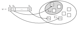
(a) Mapping of $w$ under the OWF $f$

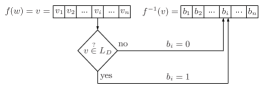
(b) Inversion of the mapping

Figure 1: OWF construction idea

The tricky part is of course the sampling, since we cannot plainly draw random elements and test membership in $L_{D}$, since this would take more than polynomial time (by construction of $L_{D}$). To mitigate this, we change $L_{D}$ into a language $\mathcal{L}_{N}$ of $N$-element sets of words, redefining the decision problem as $W\in\mathcal{L}_{N}\iff W\cap L_{D}\neq\emptyset$. That is, an element $W$ as being a set of words, is in $\mathcal{L}_{N}$ if and only if at least one of its members is from $L_{D}$, but we do not demand any knowledge about which element that is.

The so-constructed language $\mathcal{L}_{N}$ has the following properties (proven as Lemma 4.11):

1. It is at least as difficult to decide as $L_{D}$, since to decide $W\stackrel{{\scriptstyle?}}{{\in}}\mathcal{L}_{N}$, we either have to classify one entry in $W$ as being from $L_{D}$, or otherwise certify that all elements in $W$ are outside $L_{D}$ (equally difficult as deciding $L_{D}$, since deterministic complexity classes are closed under complement).

2. The property $W\in\mathcal{L}_{N}$ is monotone, in the sense that $W\in\mathcal{L}_{N}$ implies $V\in\mathcal{L}_{N}$ for all $V\supseteq W$.

The monotony admits the application of a fact that originally rooted in random graph theory (Theorem 4.12), which informally says that “every monotonous property has a threshold”. Intuitively (with a formal definition of the threshold function being part of the full statement of Theorem 4.12), a threshold is a function $m$, whose purpose is most easily explained by resorting to an urn experiment: consider an urn of $N$ balls in total, $n$ among them being white and $N-n$ balls being black. The threshold depends on $N$ and $p=n/N$, and relates to drawing from the urn without replacement as follows:

• If we draw (asymptotically) less than $m(N,p)$ balls from the urn, then the chance to get a white ball asymptotically vanishes as $N\to\infty$.

• If we draw (asymptotically) more than $m(N,p)$ balls from the urn, then the probability to get at least one white ball goes to 1 as $N\to\infty$.

Now, let us apply this idea to our sampling problem above:

• White balls represent yes-instances, i.e., word from $L_{D}$, and black balls represent no-instances, i.e., words from $\overline{L_{D}}$.

• The urn is a subset of $\Sigma^{*}$ of size $N$. To meaningfully define such sets with given size, we use a Gödel numbering of words and define our urn to contain $N$ words corresponding to the Gödel numbers $1,2,\ldots,N$. When $m$ denotes the threshold, we can get good chances to draw:

  • a yes-instance $W$ (with at least one word from $L_{D}$ in it), by taking more than $m$ words,

  • a no-instance $W$ (having $W\cap L_{D}=\emptyset$), by taking less than $m$ words.

The important observation here is that the assurance of having a yes- or no-instance is given without any explicit testing, yet at the cost of being only probabilistic. As a technical detail, we need to assure that whether we have a yes- or no-instance must not become visible by the size of $W$. This is easily assured by exploiting some sort of relativity: since the threshold depends on the size of the urn, we can under- or overshoot it by varying the size of the urn, while leaving the number $\left|W\right|$ of elements constant. This creates equally sized instances $W$ in both cases, with their answer only determined by the size of the urn; an information that does not show up in the output of our OWF.

Asymptotically, we are almost there, since we already have some useful properties:

• We can sample yes- and no-instances with probability 1 (asymptotically),

• without having to decide $L_{D}$ or $\mathcal{L}_{N}$ explicitly, and

• the sampling could (yet to be verified) run in polynomial time, provided that the threshold function behaves properly.

So, our next task is working out the threshold function, which depends on the frequency of words from $L_{D}$ occurring along the (canonic) enumeration of $\Sigma^{*}$ induced by the Gödel numbering. Alas, the diagonalization argument that gives us the (initial) language $L_{D}$ is non-constructive and in particular gives no clue on how often words from $L_{D}$ appear in $\Sigma^{*}$.

Remark 3.1.

Here, in throughout the rest of this work, when we talk about the “scattering” of a language $L$, we mean the exact locations of its words on the line $\mathds{N}$ of integers. Likewise, the “density” of $L$ merely counts the absolute frequency of words in $L$ up to a certain limit.

Towards getting an approximate count of words in $L_{D}$ inside the set of $N$ words with Gödel numbers $1,2,\ldots,N$, we use a trick: we intersect $L_{D}$ with a language of known density (formally defined in Section 3.2) that is reducible to $L_{D}$. Our language of choice contains all square integers, and defines a new base language $L_{0}=L_{D}\cap SQ$ for $\mathcal{L}_{N}$. This language is at least as hard to decide as $L_{D}$ (Lemma 4.10) and will replace $L_{D}$ in the above construction. It has some important new features:

• It gives upper bounds (Lemma 4.7) on the number of words up to Gödel number $N$ (trivially, since there cannot be more words in $L_{D}\cap SQ$ than in $SQ$, and the latter count is simple).

• It also gives lower bounds on the word count, based on a polynomial reduction of $SQ$ to $L_{D}$, illustrated in Figure 4.

With this, we can complete the sampling procedure along the following steps (expanded in Section 4.5):

1. Work out the threshold function explicitly (in fact, we will derive upper and lower bounds for it in expression (21))

2. Analyze the growth of the threshold function to assure that the number of words predicted for the sampling is meaningful (assured by (25) from below, and by (21) from above). Our use of the Gödel number in connection with the threshold bounds lets us choose the urn size polynomial in the length of the input word, so that the overall sampling algorithm (sketched next) runs in polynomial time (Lemma 4.14).

3. Define the sampling algorithm based on the aforementioned urn experiment as follows:

   • For a no-instance, make the urn “large”, such that a selection of $\left|W\right|=k$ elements will (with probability $\to 1$) not contain any word from $L_{0}$ (“white ball”).

   • For a yes-instance, make the urn “small” (relative to $k$), such that among $\left|W\right|=k$ elements, we have a high probability $(\to 1)$ of getting a word from $L_{0}$.

We call this procedure threshold sampling. It allows to realize the mapping depicted in Figure 1, and leaves the mere task of verifying the properties of an OWF according to Definition 2.3. The evaluation of the function in polynomial time means to repeatedly sample, each run taking polynomial time (in the number of bits). This will directly become visible in the construction and from the properties of the threshold.

Showing the intractability of inversion is trickier, but here we can make use of the fact that Definition 2.1 does not require the function to be bijective. In fact, the use of randomness in the sampling necessarily renders our constructed mapping not bijective, but any inversion algorithm working on the image $y=f(b_{1}b_{2}\ldots b_{n})$ would necessarily also return a correct first bit $b_{1}$. Taking a contraposition, this means that the chances for the inversion to fail are at least those to screw up the computation of $b_{1}$ (the argument is expanded in full detail in Section 4.8). But this is exactly how the diagonal language $L_{D}$ was constructed for, in the worst case. So our last challenge is making the worst-case appear with the desired frequency of $1-1/\text{poly}(n)$, as required for a weak OWF. This is done by modifying the encoding of Turing machines to use only a logarithmically small fraction of its input, so as to consider a large number of inputs of the same length as equivalent (in Section 5, we will relate this to the notion of local checkability [3]). This (wasteful) encoding is consistent with all relevant definitions (especially Definition 2.1), but makes the worst-case occur with a non-negligible frequency (as we require).

Having outlined all ingredients, let us now turn to the formal details, starting with some preparation.

3.1 Gödel Numbering

To meaningfully associate subsets $\left\{1,2,\ldots,N\right\}\subset\mathds{N}$ with subsets of $\Sigma^{*}$, let us briefly recall the concept of a Gödel numbering. This is a mapping $gn:\Sigma^{*}\to\mathds{N}$ that is computable, injective, and such that $gn(\Sigma^{*})$ is decidable and $gn^{-1}(n)$ is computable for all $n\in\mathds{N}$ [10]. The simple choice of $gn(w)=(w)_{2}$ is obviously not injective (since $(0^{n}w)_{2}=(w)_{2}$ for all $n\in\mathds{N}$ and all $w\in\Sigma^{*}$), but this can be fixed conditional on $0\notin\mathds{N}$ by setting

$$gn(w):=(1w)_{2}.$$ (2)

This is the Gödel numbering that we will use throughout the rest of this work, and it is not difficult to verify the desired properties as stated above. Most importantly, (2) is a computable bijection between $\mathds{N}$ and $\Sigma^{*}$.

For the Gödelization of TMs, let $\rho(M)\in\Sigma^{*}$ denote a complete description of a TM $M$ in string form (using some prefix-free encoding to denote the alphabet, state transitions, etc.). The encoding that we will use (and define in Section 4.2) will have the following properties (as are commonly required; cf. [2, 11]):

1. every string over $\left\{0,1\right\}^{*}$ represents some TM (easy to assure by executing an invalid code as a canonic TM that instantly halts and rejects its input),

2. every TM is represented by infinitely many strings. This is easy by introducing the convention to ignore a prefix of the form $1^{*}0$ then the string representation is being executed.

The Gödelization of a TM $M$, represented as $\rho(M)\in\Sigma^{*}$, is then the integer $gn(\rho(M))$.

3.2 Density Functions

For a language $L$, we define its density function, w.r.t. a Gödel numbering $gn$, as the mapping

$$\text{dens}_{L}:\mathds{N}\to\mathds{N},\quad x\mapsto\left|\left\{w\in L:gn(w)\leq x\right\}\right|,$$

i.e., $\text{dens}_{L}(x)$ is the number of words whose Gödel number as defined by (2) is bounded by $x$. The dependence of $\text{dens}_{L}$ on the Gödel numbering $gn$ can be omitted hereafter, since there will be no second such numbering and hence no ambiguity by this simplification of the notation.

Occasionally, it will be convenient to let $\text{dens}_{L}$ send a word $v\in\Sigma^{*}$ to an integer $\mathds{N}$, in which case we put $x:=gn(v)=(1v)_{2}$ in the definition of $\text{dens}_{L}$ upon an input word $v$. The density of the language $L$ will be our technical vehicle to quantify (bound) the likelihood of drawing an element from $L$ within a bounded set of integers $\left\{1,2,\ldots,n\right\}$ (see Lemma 4.1 below), where the bound $n$ will be an integer or a binary number coming as a string (whichever is the case will be clear from the context).

4 Proof of Theorem 2.4

The proof will cook up a weak OWF from the ingredients outlined in Section 3, in almost bottom up order.

4.1 Properties of Density Functions

Our first subgoal is the ability to construct random yes- and no-instances of a difficult decision problem. So, we first need to relate the density function for a language $L$ to the likelihood of retrieving elements from it upon uniformly random draws.

Lemma 4.1.

For every language $L$, the density function satisfies $\text{dens}_{L}(x)\leq x$ for all $x\in\mathds{N}$.

Proof.

Assume the opposite, i.e., the existence of some $x_{0}$ for which $\text{dens}_{L}(x_{0})>x_{0}$. In that case, there must be at least $x_{0}+1$ words $w_{1},w_{2},\ldots,w_{x_{0}+1}$ in $L$ for which $gn(w_{i})\leq x_{0}$ for all $i=1,2,\ldots,x_{0}+1$. W.l.o.g., let $w_{1}$ be the word whose Gödel number $gn(w_{1})$ is maximal. Since $gn$ is injective, all other $x_{0}$ words map to distinct smaller integers, thus making $gn(w_{1})\geq x_{0}+1$ at least. This clearly contradicts our assumption that $gn(w_{1})\leq x_{0}$. ∎

Lemma 4.1 permits the use of the density function to define an urn experiment as follows: let the urn be $U=\left\{1,2,\ldots,n\right\}\subset\mathds{N}$, and let each element in it correspond to a word $w\in\Sigma^{*}$ by virtue of $gn^{-1}$. Then the likelihood to draw an element from $L$ addressed by a random index in $U$ is $\text{dens}_{L}(n)/n$, by counting the number of positive cases relative to all cases.

To illustrate the practical use of a density function, let us consider the following example of a language that we will heavily use throughout this work. The language of integer squares is defined as $SQ=\{y:\exists x\in\mathds{N}$ such that $y=x^{2}\}$. Each element $y\in SQ$ can be identified with a string (in regular expression notation) $w_{y}\in 1(0\cup 1)^{*}\subset\Sigma^{*}$, for which $y=(w_{y})_{2}$. The Gödel number of $w_{y}$ can be computed from $y$ by $gn(w_{y})=2^{\left\lceil\log y\right\rceil+c(y)}+y$, with the padding function

$$c(y)=\left\{\begin{array}[]{ll}0,&\hbox{if }\log y<\left\lceil\log y\right\rceil;\\ 1,&\hbox{if }\log y=\left\lceil\log y\right\rceil.\end{array}\right.$$

Let us extend our definition of $gn$ to a mapping from $\mathds{N}\to\mathds{N}$, where $gn(y)$ for $y\in\mathds{N}$ is defined as $gn(y):=gn(w_{y})$ with $y=(w_{y})_{2}$. Using the previous formula to compute $gn(y)$, note that the expression

$$\frac{gn(y)}{y}=\frac{2^{\left\lceil\log y\right\rceil+c(y)}+y}{y}=1+\frac{2^{\left\lceil\log y\right\rceil+c(y)}}{y},$$

ultimately becomes numerically trapped within the interval $[1,5]$ for $y\to\infty$ (the lower bound is immediate; the upper bound follows from $2^{\left\lceil\log y\right\rceil+c(y)}\leq 2^{1+(\log y)+1}=4y$). Thus,

$$y\leq gn(y)\leq 5\cdot y\quad\text{for sufficiently large}~{}y.$$ (3)

Moreover, it is easy to see that for $z,x\in\mathds{N}$,

$$\left|\left\{z^{2}:z^{2}\leq x\right\}\right|=\left\lfloor\sqrt{x}\right\rfloor.$$ (4)

Using both facts, we discover that for any two $x,z\in\mathds{N}$ that satisfy $gn(z^{2})\leq x$, also $z^{2}\leq gn(z^{2})\leq x$ holds by (3). Thus, $[gn(z^{2})\leq x]\Rightarrow[z^{2}\leq x]$ and hence $\left\{z^{2}:gn(z^{2})\leq x\right\}\subseteq\left\{z^{2}:z^{2}\leq x\right\}$. The cardinalities of these sets satisfy the respective inequality, and (4) gives

$$\text{dens}_{SQ}(x)\leq\left\lfloor\sqrt{x}\right\rfloor\leq\sqrt{x}.$$ (5)

Conversely, $gn(z^{2})\leq 5z^{2}$ asymptotically by (3) means that for sufficiently large $z$, $gn(z^{2})\leq 5\cdot z^{2}\iff\frac{1}{5}\cdot gn(z^{2})\leq z^{2}$. Thus, $[z^{2}\leq x]\Rightarrow[\frac{1}{5}\cdot gn(z^{2})\leq x]$, and the last condition is equivalent to $gn(z^{2})\leq 5\cdot x$. Therefore, $\left\{z^{2}:z^{2}\leq x\right\}\subseteq\left\{z^{2}:gn(z^{2})\leq 5\cdot x\right\}$, and the cardinalities satisfy the respective inequality. It follows that $\text{dens}_{SQ}(5\cdot x)\in\Omega(\sqrt{x})$, or after substituting and renaming the variables, $\text{dens}_{SQ}(x)\in\Omega(\sqrt{x})$.

Summarizing our findings, we have proven:

Lemma 4.2.

The language of squares $SQ=\left\{y:y=x^{2},x\in\mathds{N}\right\}$ has a density function $\text{dens}_{SQ}(x)\in\Theta(\sqrt{x})$.

As announced in Section 3, we will later look at the density of the intersection of two languages (namely $L_{D}\cap SQ$, where $L_{D}$ has not been constructed explicitly yet). The definition of density functions immediately delivers a useful inequality for such intersection sets: for every two languages $L_{1},L_{2}$, we have

$$\text{dens}_{L_{1}\cap L_{2}}\leq\text{dens}_{L_{1}},$$ (6)

since there cannot be more words in $L_{1}\cap L_{2}$ than words in $L_{1}$ (or $L_{2}$, respectively). This will enable us to bound the density of the (more complex) intersection language in terms of the simpler (and known) density of $SQ$. Details will be postponed until a little later.

4.2 Encoding of Turing Machines

As a purely technical matter, we will adopt a specific encoding convention for TMs. While the following facts are almost trivial, it is important to establish them a-priori (and thus independently) of our upcoming arguments, since the scattering and density of the languages that we construct will depend on the chosen encoding scheme of TMs. Specifically, we will encode a TM $M$ into a string $\rho(M)$ as outlined in Section 3.1, with a few adaptations when it comes to executing a code for a TM:

• When a TM as specified by an input $w\in\Sigma^{*}$ is to be executed by a universal TM $M_{U}$, then the code $\rho(M)$ that defines $M$’s actions is obtained by $M_{U}$ as follows:

  • the input $w$ is treated as an integer $x=(w)_{2}$ in binary and all but the most significant $\left\lceil\log(\mathop{\text{len}}\left(w\right))\right\rceil$ bits are ignored. Call the resulting word $w^{\prime}$.

  • from $w^{\prime}$, we drop all preceding $1$-bits and the first 0-bit, i.e., if $w^{\prime}=1^{k}0v$, then $\rho(M)=v$ after discarding the prefix padding $1\ldots 10$.

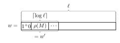
Figure 2: Encoding of Turing machines with padding

Although this encoding – depicted in Figure 2 – is incredibly wasteful (as the code for a TM is taken as padded with an exponential lot of bits), it assures several properties that will become useful at the beginning and near the end of this work:

1. The aforementioned mapping $w\mapsto w^{\prime}$ shrinks the entirety of $2^{\ell}$ words in $\left\{0,1\right\}^{\ell}$ down to only $2^{\left\lceil\log\ell\right\rceil}\geq\ell$ distinct prefixes. Each of these admits a lot of $2^{\ell-\left\lceil\log\ell\right\rceil}$ suffixes that are irrelevant for the encoding of the TM. Thus, an arbitrary word $w^{\prime}$ encoding a TM has at least

   $$2^{\ell-\left\lceil\log\ell\right\rceil}\geq 2^{\ell-\log\ell-1}$$ (7)

   equivalents $w$ in the set $\left\{0,1\right\}^{\ell}$ that map to $w^{\prime}$. Thus, if a TM $M$ is encoded within $\ell$ bits, then (7) counts how many equivalent codes for $M$ are found at least in $\left\{0,1\right\}^{\ell}$. This will be used in the concluding Section 4.8, when we establish failure of any inversion circuit in a polynomial number of cases (second part of Definition 2.1).

2. The retraction of preceding $1$-bits creates the needed infinitude of equivalent encodings of every possible TM $M$, as we can embed any code $\rho(M)$ in a word of length $\ell$ for which $\log(\ell)>\mathop{\text{len}}\left(\rho(M)\right)$. We will need this to prove the hierarchy theorem in Section 4.3.

Remark 4.3.

Note that exponential difference in the size of $\rho(M)$ and its representation $w$ in fact does not preclude the efficient execution of $w$ as input code and data to the universal TM, because it only executes a logarithmically small fraction of its input code. Conversely, the redundancy of our encoding only means that we have to reach out exponentially far on $\mathds{N}$ to see the first occurrence of a TM with a code of given size; this is, however, not forbidden by any of the relevant definitions.

Let $\mathcal{TM}=\left\{M_{1},M_{2},M_{3},\ldots\right\}$ be an enumeration of all TMs under the encoding just described; that is, $\mathcal{TM}$ is the set of all $w\in\Sigma^{*}$ for which a TM $M$ with encoding $\rho(M)$ exists that is embedded inside $w$ as shown in Figure 2. Observe that the first $1$-bit (mandatory in our encoding) when being stripped from a word $w$ by $gn^{-1}$ leaves the inner representation of $M$ intact (since the $1^{+}0$-prefix is ignored for the “execution” of $w$ anyway). We write $M_{w}$ to mean the TM encoded by $w$.

A simulation by the universal TM $M_{U}$ thus takes the program $w$ and input $x$ to act on the initial tape configuration $\#w\#x\underline{\#}$, or in expanded form (cf. Figure 2),

$$\#\underbrace{1^{+}0}_{\begin{subarray}{c}\text{padding}\\ \text{(ignored)}\end{subarray}}\overbrace{\rho(M)}^{\text{code}}\underbrace{(0\cup 1)^{*}}_{\begin{subarray}{c}\text{padding}\\ \text{(ignored)}\end{subarray}}\#x\underline{\#}$$ (8)

where $\#$ marks spaces on the tape, and the head position is marked by the underlining.

4.3 A Review of the Time Hierarchy Theorem

Returning to the proof outline, our next goal is to find a proper difficult language $L_{D}$ that we can use for the encoding of input bits into yes/no instances of a decision problem. To this end, it is useful to take a close look at the proof of the deterministic time hierarchy theorem known from complexity theory. The theorem’s hypothesis is summarized as follows:

Assumption 4.4.

Let $T:\mathds{N}\to\mathds{N}$ be a fully time-constructible function, and let $t:\mathds{N}\to\mathds{N}$ with $t(n)\geq n$ be a monotonously increasing function for which

$$\lim_{\ell\to\infty}\frac{t(\ell)\cdot\log t(\ell)}{T(\ell)}=0.$$

Theorem 4.6 is obtained by diagonalization [11, Thm.12.9]: we construct a TM $M$ that halts within no more than $T(\mathop{\text{len}}\left(w\right))$ steps upon input of a word $w$ of length $\ell$, and differs in its output from every other TM $M^{\prime}$ that is $t(\ell)$-time-limited.

On input of a word $w$ of length $\ell=\mathop{\text{len}}\left(w\right)$, the sought TM $M$ will employ a universal TM $M_{U}$ to simulate an execution of $M_{w}$ on input $w$. The simulation of $t(\ell)$ steps of $M_{w}$ can be done by $M$ taking no more than $c_{M_{w}}\cdot t(\ell)\log t(\ell)$ steps [11, Thm.12.6], where $c_{M_{w}}$ is a constant that depends only on the number of states, tapes, and tape-symbols that $M_{w}$ uses, but not the length of the input to ($M_{U}$’s simulation of) $M_{w}$.

To assure that $M$ always halts within the limit $T(\ell)$, it simultaneously executes a “stopwatch” TM $M_{T}$ on the input $w$, which exists since $T$ is fully time-constructible. Once $M_{T}$ has finished, $M$ terminates the simulation of $M_{w}$ too, and outputs “accept” if and only if two conditions are met:

1. $M_{w}$ halted (by itself) during the simulation (i.e., it was not interrupted by the termination of $M_{T}$), and,

2. $M_{w}$ rejected $w$.

The “diagonal-language” $L_{D}$ is thus defined over the alphabet $\Sigma=\left\{0,1\right\}$ as

$$L_{D}:=\left\{w\in\Sigma^{*}:M_{w}\text{ halts and rejects }\rho(M_{w})\text{ within}\leq T(\mathop{\text{len}}\left(\rho(M_{w})\right))\text{ steps}\right\}.$$ (9)

Remark 4.5.

Textbook proofs of the time hierarchy theorem, e.g., [11], adopt a slightly simpler version of $L_{D}$, usually a word $w$ entirely be interpreted as some code for a TM $M_{w}$, and having this TM process $w$ within time $T(\mathop{\text{len}}\left(w\right))$. In foresight of our intention to “pad” words into becoming perfect squares (to lie in a (modified version of) $SQ$), this padding would change $w$ into some different word $w^{\prime}$, but leave the “functional prefix” $\rho(M)$ (see Fig. 2) inside $w$ unchanged. Hence, $M_{w}$ would not simulate its own code, but a modified version thereof. To recover the arguments for the textbook proof of the hierarchy theorem, we restrict the decision to processing only that part of $w$ that contains the TM encoding, i.e., $w^{\prime}$ in Fig. 2. Since we still retain the infinitude of equivalent encodings by the prefix $1^{+}0$ in Fig. 2, the proof arguments from the textbook [11] remain intact.

The hierarchy theorem is then found by observing that $L_{D}$ cannot be accepted by any $t$-time-limited TM $M$: If $M$ were $t$-time-limited with encoding $\rho(M)=w^{\prime}$, then the list $\mathcal{TM}$ contains another (equivalent) encoding $w$ of length $\ell=\mathop{\text{len}}\left(w\right)$ so that $M=M_{w^{\prime}}$ and $M_{w}$ compute identical functions, and for sufficiently large $\ell$,

$$c_{M_{w}}\cdot t(\ell)\cdot\log t(\ell)\leq T(\ell),$$ (10)

so that $M_{w}$ can carry to completion within the time limit $T(\ell)$. Now, $w\in L(M_{w})$ if and only if $w\notin L_{D}$, so that $L_{D}\neq L(M_{w})$. Since $M$ was $t$-time-limited and arbitrary, and $M_{w}$ decides the same language as $M$, we have $L_{D}\neq L(M)$ for all $M$ that are $t$-time-limited, and therefore $\textsc{Dtime}(t)\subsetneq\textsc{Dtime}(T)$ if also $t\leq T$.

At this point, we just re-proved the following well-known result:

Theorem 4.6 (deterministic time hierarchy theorem).

Let $t,T$ be as in Assumption 4.4 and $t\leq T$, then $\textsc{Dtime}(t)\subsetneq\textsc{Dtime}(T)$.

4.4 A Hard Language with a Known Density Bound

The existence of a language $L_{D}$ that is hard to decide allows the construction of another language whose scattering over $\Sigma^{*}$ can be quantified explicitly. We will intersect $L_{D}$ with another language with known density estimates, and show that the hardness of the implied decision problem is retained. Our language of choice will be already known set of integer squares that we will (equivalently) redefine for that purpose to be $SQ:=\{w\in\Sigma^{*}:\exists x\in\mathds{N}$ such that $gn(w)=x^{2}\}$. This language has a density $\text{dens}_{SQ}(x)\in\Theta(\sqrt{x})$ by Lemma 4.2.

We claim that the language

$$L_{0}:=L_{D}\cap SQ$$

is at least as difficult to decide as $L_{D}$. Assume the opposite $L_{0}\in\textsc{Dtime}(t)$ towards a contradiction, and let a word $w\in\Sigma^{\ell}$ be given. Without loss of generality, let us assume that the lower order bits in $w$ are all zero, since the relevant “functional” part is the header $1^{+}\rho(M)$ (cf. (8)).

We look for the smallest $w^{\prime}\geq w$ that approximates $w$ from above and represents a square number in binary, which is $(w^{\prime})_{2}=\left\lceil\sqrt{(w)_{2}}\right\rceil^{2}\geq(w)_{2}$. Observe that two adjacent integer squares $x^{2}$ and $(x+1)^{2}$ are separated by no more than $(x+1)^{2}-x^{2}=2x+1$. Therefore, putting $x=\left\lceil\sqrt{(w)_{2}}\right\rceil$, we find that the difference $\Delta$ between $w$ and its upper square approximation $w^{\prime}$ satisfies $(w^{\prime})_{2}-(w)_{2}=\Delta\leq 2\left\lceil\sqrt{(w)_{2}}\right\rceil+1$. Taking logarithms to get the bitlength, we find that $\Delta$ takes no more than $\left\lceil\log(2\left\lceil\sqrt{(w)_{2}}\right\rceil+1)\right\rceil\leq 3+\frac{1}{2}\left\lceil\log(w)_{2}\right\rceil=3+\frac{\mathop{\text{len}}\left(w\right)}{2}$ bits, assuming that $w$ has no leading zeroes (which our Gödel numbering precludes).

By adding $\Delta$ to $(w)_{2}$ to get the sought square $(w^{\prime})_{2}=(w)_{2}+\Delta$, note that the shorter bitlength of $\Delta$ relative to the bitlength of $w$ makes $w$ and $w^{\prime}$ different in the lower half + 4 bits (including the carry from the addition of $\Delta$). Equivalently, $w$ and $w^{\prime}$ have a Hamming distance $\leq\frac{1}{2}\mathop{\text{len}}\left(w\right)+4$.

Since $\ell-\log(\ell)>4+\frac{1}{2}\ell$ for sufficiently large $\ell$, we conclude that $w$ and its “square approximation” $w^{\prime}$ will eventually have an identical lot of $\left\lceil\log\ell\right\rceil$ most significant bits (cf. Figure 2). That is, the header of the word that is relevant for $L_{D}$ is not touched when $w$ is converted into a square $w^{\prime}$. This means that $w\in L_{D}\iff w^{\prime}\in L_{D}$, so that the decision remains unchanged upon the switch from $w$ to $w^{\prime}$. Since $w^{\prime}\in SQ$ holds by construction, we could decide $w\in L_{D}$ by deciding whether $w^{\prime}\in L_{D}\iff w^{\prime}\in L_{D}\cap SQ$, so that $L_{D}\in\textsc{Dtime}(t)$ by our initial hypothesis on $L_{0}$ and the additional assumption that $t(n)\geq n^{3}$. This contradiction puts $L_{0}\notin\textsc{Dtime}(t)$, as claimed. To retain $L_{D}\cap SQ\in\textsc{Dtime}(T)$, we must choose $T$ so large that the decision $w\in SQ$ is possible within the time limit incurred by $T$, so we add $T(n)\geq n^{3}$ to our hypothesis besides Assumption 4.4 (note that we do not need an optimal complexity bound here).

Using (6) with $L_{1}=L_{D}$ and $L_{2}=SQ$, we see that for sufficiently large $x$,

$$\text{dens}_{L_{0}}(x)=\text{dens}_{L_{D}\cap SQ}(x)\leq\text{dens}_{SQ}(x)\leq\sqrt{x},$$

by (5). This proves half of what we need, so let us capture this intermediate finding in a rememberable form:

Lemma 4.7.

Let $t,T$ be as in Assumption 4.4 and assume $T(n)\geq t(n)\geq n^{3}$. Then, there exists a language $L_{0}\in\textsc{Dtime}(T)\setminus\textsc{Dtime}(t)$ for which

$$\text{dens}_{L_{0}}(x)\leq\sqrt{x}.$$

Towards a lower bound for the density, the following observation will turn out as a key tool:

Lemma 4.8.

The language $L_{0}$ described in Lemma 4.7 is $\textsc{Dtime}(t)$-hard (via polynomial reduction).

Proof.

We need to show that for every $L\in\textsc{Dtime}(t)$, there exists a poly-time reduction $\varphi$ to the language $L_{0}$. Remember that by definition (9), $L_{D}$ is the set of all words $w$ that when being interpreted as an encoding of a Turing machine $M_{w}$, this machine would reject “itself” as input within time $T(\mathop{\text{len}}\left(w\right))$.

Take any $L\in\textsc{Dtime}(t)$, then there is a TM $M_{L}$ that decides $w\stackrel{{\scriptstyle?}}{{\in}}L$ in time $t(\mathop{\text{len}}\left(w\right))$. Let $M_{\overline{L}}$ be the TM that decides $\overline{L}$ (i.e., by simply inverting the answer of $M_{L}$). To construct a proper member of $L_{D}\cap SQ$ that equivalently delivers this answer, we define the reduction $\varphi(w)=w^{\prime}=\rho(M_{\overline{L}})\$w\$0^{\nu}$ for an integer $\nu$ that is specified later. That is, the word $w^{\prime}$ contains a description of $M_{\overline{L}}$, followed by the original input $w$ and a number $\nu$ of trailing zeroes that will later be used to cast this word into a square. The three blocks in $\varphi(w)$ are separated by $-symbols, assuming that $ is not used in any of the relevant tape alphabets, and we use a prefix-free encoding.

Let us collect a few useful observations about the mapping $\varphi$:

• $\varphi(w)$ is poly-time computable when $\nu=\text{poly}(\mathop{\text{len}}\left(w\right))$, since $\rho(M_{\overline{L}})$ is merely a constant prefix being attached. It is especially crucial to remark here that the exponential expansion of a TM of length $\ell$ into an encoding of size $O(2^{\ell})$ (cf. Remark 4.3) does not make the complexity to evaluate $\varphi$ exponential, since the universal TM $M_{U}$ merely drops padding from the code, but not from the entire input word. Indeed, the (padded) code $1^{+}0\rho(M_{\overline{L}})1^{*}(0\cup 1)^{*}$ appearing on the TM’s tape (see (8)) is exponentially longer than the “pure” code for $M_{\overline{L}}$, but it is nevertheless a constant prefix used by the reduction $\varphi$, since it is constructed explicitly for the fixed language $L$. As such, the reduction is doable in $O(1)$ time.

  A slight difficulty arises from the need to make $\varphi(w)=w^{\prime}$ sufficiently long to give the simulation of $M_{w^{\prime}}$ enough time to finish. This is resolved by increasing $\nu$ (thus making the zero-trailer $0^{\nu}$ longer), so as to enlarge $w^{\prime}$ until condition (10) is satisfied. Note that the increase of $\nu$ depends on $t$ and $T$ only and is as such a fixed number (constant), adding to the remainder length of $\nu$ that polynomially depends on the length of $w\in L$ only.

• The output length $\mathop{\text{len}}\left(\varphi(w)\right)$ is again polynomial in $\mathop{\text{len}}\left(w\right)$ under the condition that $\nu=\text{poly}(\mathop{\text{len}}\left(w\right))$.

• $\varphi$ is injective, since $w_{1}\neq w_{2}$ implies $\varphi(w_{1})\neq\varphi(w_{2})$ by definition.

To see why $w\in L\iff\varphi(w)=w^{\prime}\in L_{D}$, let us agree on the convention that the TM $M_{\varphi(w)}$ executes $M_{\overline{L}}$ only on that part of $w^{\prime}$ that is enclosed within $-symbols. Leaving our universal TM unmodified, this restriction can be implemented by a proper modification of $M_{\overline{L}}$ to ignore everything before and after the $-symbols during its execution (thus slightly changing the definition of our reduction to respect this). Let us call the so-modified TM $M^{\prime}_{\overline{L}}$, and alter the reduction into $\varphi(w):=\rho(M^{\prime}_{\overline{L}})\$w\$0^{\nu}$.

Under these modifications, it is immediate that:

1. the simulation of $M_{w^{\prime}}$ on input $w^{\prime}$ is actually a simulation of $M_{\overline{L}}$ on input $w$, and has – by construction (a suitably large padding of $\nu$ trailing bits) – enough time to finish, and,

2. the TM deciding $L_{D}$ will accept $w^{\prime}$ if and only if $M_{\overline{L}}$ rejects $w$. In that case, however, $M_{L}$ would have accepted $w$, thus $w\in L\iff\varphi(w)\in L_{D}$.

It remains to modify our reduction a last time to assure that $\varphi(w)\in SQ$ for every possible $w$, so as to complete the reduction $L\leq_{p}L_{0}$. For that matter, we will utilize the previously introduced trailer of zeroes $0^{\nu}$ in $\varphi(w)$.

Define the number $k:=\mathop{\text{len}}\left(\rho(M^{\prime}_{\overline{L}})\$w\$\right)=c+\mathop{\text{len}}\left(w\right)$, where $c$ is a constant that counts the length of $\rho(M^{\prime}_{\overline{L}})$ and the $-symbols when everything is encoded in binary. We will enforce $\varphi(w)\in SQ$ by interpreting $w^{\prime}=\rho(M^{\prime}_{\overline{L}})\$w\$0^{\nu}$ as a binary number with $\nu$ trailing zeroes, and add a proper value to it so as to cast $w^{\prime}$ into the form $(w^{\prime})_{2}=x^{2}$ for some integer $x$. The argument is exactly as in the proof of Lemma 4.7, and thus not repeated but visualized in Figure 3.

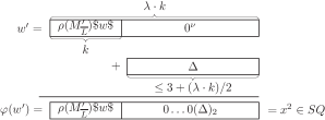
Figure 3: Mapping into the set of squares

Now, let $\nu$ be such that $\mathop{\text{len}}\left(w^{\prime}\right)=\lambda\cdot k$ for some (sufficiently large) integer multiple $\lambda\geq 3$ (see Figure 3 to see how $\nu,\mathop{\text{len}}\left(w^{\prime}\right),k$ and $\lambda$ are related). To cast $\varphi(w)$ into the sought form $(\varphi(w))_{2}=x^{2}$ for an integer $x\in\mathds{N}$ (and hence $\varphi(w)\in SQ$), we need to add some $\Delta$ towards the closest larger integer square. If we choose $\lambda$ so large that $3+\frac{\lambda}{2}\cdot k<(\lambda-1)k$, then $\nu\geq(\lambda-1)k$ zero-bits (plus the additional lot to satisfy condition (10) if necessary, but for sufficiently long words, this requirement vanishes) at the end of $w^{\prime}$ suffice to take up all bits of $\Delta$, and $(\rho(M^{\prime}_{\overline{L}})\$w\$0^{\nu})_{2}+\Delta=(\rho(M^{\prime}_{\overline{L}})\$w\$0^{*}z)_{2}$ (with $z$ being the binary representation of $\Delta$) is a square. Since $\lambda$ can be chosen as a fixed integer multiplier for $k=c+\mathop{\text{len}}\left(w\right)$, the above requirement $\nu=\text{poly}(\mathop{\text{len}}\left(w\right))$ is satisfied, and $\varphi(w)\in SQ$ holds for every input word $w$.

Therefore, $\forall w:\varphi(w)\in SQ$ implies $w\in L\iff\varphi(w)\in L_{D}\cap SQ\iff\varphi(w)\in L_{D}$, and the result follows since $L\in\textsc{Dtime}(t)$ was arbitrary. ∎

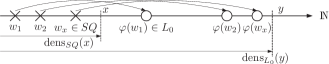
Figure 4: Illustration of inequality (11)

Lemma 4.8 lets us lower bound the number of words in $L_{0}$ by using any known lower bound for any language in $\textsc{Dtime}(t)$, and knowing that all these words map into $L_{0}$ (see Figure 4). Our language of choice will be $SQ$ once again, with Lemma 4.2 providing the necessary bounds. This is admissible if we add the hypothesis $t(n)\geq n^{3}$ so that $SQ\in\textsc{Dtime}(t)$. Furthermore, Assumption 4.4 then implies that $T(n)\in\Omega(n^{3})$ as well, so that this requirement in Lemma 4.7 becomes redundant under our so-extended hypothesis.

We consider the length of a word $w$ being mapped to a word $\varphi(w)\in L_{0}=L_{D}\cap SQ$. For $x\in\mathds{N}$, let $w_{x}$ be the last word to appear before $x$ in an ascending $\leq$-ordering of $SQ$ (see Figure 4). The mapping $\varphi$ is strictly increasing in the following sense: the images of two words $w_{1}\leq w_{2}$ under $\varphi$ would contain $w_{1},w_{2}$ as “middle” blocks in the bitstrings $\varphi(w_{1}),\varphi(w_{2})$, where they determine the order $gn(\varphi(w_{1}))\leq gn(\varphi(w_{2}))$: if $\mathop{\text{len}}\left(w_{1}\right)<\mathop{\text{len}}\left(w_{2}\right)$, then $\mathop{\text{len}}\left(\varphi(w_{1})\right)<\mathop{\text{len}}\left(\varphi(w_{2})\right)$ and the order is the same as that of $w_{1}$ and $w_{2}$. Otherwise, if $w_{1}$ and $w_{2}$ have the same length, then the prefixes of $\varphi(w_{1})$ and $\varphi(w_{2})$ also match, and the lower-order bits contributed by the individual $\Delta$ cannot change the numeric ordering, thus leaving the order of the images to be determined by the order of $w_{1},w_{2}$. This means that $w\leq w_{x}$ implies $\varphi(w)\leq\varphi(w_{x})$, so that we find

$$\text{dens}_{SQ}(gn(w))\leq\text{dens}_{L_{0}}(gn(\varphi(w))).$$ (11)

We shall use (11) to lower-bound $\text{dens}_{L_{0}}(y)$ asymptotically for sufficiently large $y\in\mathds{N}$. To this end, let us change variables in inequality (11), using Figure 4 with $L=SQ$ to guide our intuition: Equivalently to letting $y$ be arbitrary, we can take an arbitrary word $w^{\prime}\in\Sigma^{*}$ to define $y$ as $y:=gn(w^{\prime})$. Since $\varphi$ is not surjective, we cannot hope to find a preimage for every $w^{\prime}\in\Sigma^{*}$, so we distinguish two cases:
Case 1 ($y=gn(\varphi(w))$ for some $w\in\Sigma^{*}$): The preimage $w$ of $w^{\prime}$ under $\varphi$ is unique since the reduction is injective. By substitution, we get

$$\text{dens}_{SQ}(gn(\varphi^{-1}(w^{\prime})))\leq\text{dens}_{L_{0}}(gn(w^{\prime})).$$ (12)

For such a $w^{\prime}=\rho(M^{\prime}_{\overline{SQ}})\$w\$0^{*}z$, where $w\in SQ$, it is a simple matter to extract the preimage $w$, located “somewhere in the middle” of $w^{\prime}$. Precisely, $w$ is located in the left-most $k$-bit block (among the total of $\lambda$ such blocks), and has a length equal to $\frac{1}{\lambda}\mathop{\text{len}}\left(w^{\prime}\right)-c^{\prime}$, where the constant $c^{\prime}\geq c$ accounts for the length of $\rho(M^{\prime}_{\overline{SQ}})$, the additional 1 bit from the Gödel numbering, the separator symbols $\$$, and a possible remainder of zeroes from the $0^{\nu}$-trailer (containing the $\Delta$ towards the next square).

The preimage $w=\varphi^{-1}(w^{\prime})$ satisfies

$$gn(w)\geq 2^{\mathop{\text{len}}\left(w\right)}=2^{\frac{1}{\lambda}\left\lceil\log(gn(w^{\prime}))\right\rceil-c^{\prime}}\geq 2^{-c^{\prime\prime}}\sqrt[\lambda]{gn(w^{\prime})},$$ (13)

where $c^{\prime\prime}$ is a constant again.

Substituting this into (12), we get $\text{dens}_{SQ}(2^{-c^{\prime\prime}}\sqrt[\lambda]{gn(w^{\prime})})\leq\text{dens}_{L_{0}}(gn(w^{\prime}))$. Using that $\text{dens}_{SQ}(x)\in\Theta(\sqrt{x})$ (Lemma 4.2), we end up finding that for a constant $D^{\prime}$ (implied by the $\Theta$), another constant $\beta$ (dependent on $c^{\prime\prime}$) and sufficiently long $w^{\prime}$,

$$D^{\prime}\sqrt{2^{-c^{\prime\prime}}\sqrt[\lambda]{gn(w^{\prime})}}=D\cdot\sqrt[\beta]{(w^{\prime})_{2}}\leq\text{dens}_{L_{0}}(gn(w^{\prime})),$$ (14)

where $D>0$ is yet another constant. Observe that the construction requires $\lambda\geq 3$ and therefore makes $\beta\geq 6$ (we will use this observation later).
Case 2 ($y\neq gn(\varphi(w))$ for all $w\in\Sigma^{*}$): The key insight here is that for lower-bounding the count (the density function), it suffices to identify some $w$ for which $gn(\varphi(w))<y=gn(w^{\prime})$, in which case we get a coarser bound

$$\text{dens}_{SQ}(gn(w))\leq\text{dens}_{L_{0}}(gn(\varphi(w)))<\text{dens}_{L_{0}}(y)=\text{dens}_{L_{0}}(gn(w^{\prime})),$$

where the second inequality holds since the density function is monotonously increasing. A simple and reliable way to find $w$ is the following: for the moment, let us forget about $w^{\prime}$ not being in the image set of $\varphi$, and extract a substring from it exactly like in case 1 before (disregarding that the prefix and suffix may not have the proper form as under $\varphi$). Then, we shorten the result by deleting one bit from it (say, the least significant) and call the so-obtained word $w$. Observe that $\varphi(w)$ is shorter than $w^{\prime}$, so that $gn(\varphi(w))<gn(w^{\prime})$ necessarily. But $\varphi(w)$ has the preimage $w$, so the same arguments as in the previous case can be used again, starting from (13) onwards. The only difference is the constant $c^{\prime}+1$ instead of $c^{\prime}$ (as we deleted one more bit), and the subsequently new constant $D^{\prime\prime}$ when we re-arrive at (14) (notice that $w^{\prime}$ re-occurs in that expression, since we obtained $w$ from $w^{\prime}$, and only the length of $w^{\prime}$ but not its structure played a role in (13)).

Since the bound (14) takes the same form in both cases, except for the different constants, we can choose the coarser of the two as a lower limit in all cases.

Remark 4.9.

Note that (some of) the constants involved here actually and ultimately depend (through a chain of implications) on the choices of the two functions $t$ and $T$. These give rise to the language $L_{D}$ and determine the “stopwatch” that we must attach to the simulation of $M_{\overline{SQ}}$ when reducing the language ${SQ}$ to our hard-to-decide language $L_{D}\in\textsc{Dtime}(T)\setminus\textsc{Dtime}(t)$. This in turn controls the overhead for the reduction function $\varphi$ in Lemma 4.8 and the magnitude of the constants $\lambda,\beta$, etc.

Together with Lemma 4.7, and after substituting $y=gn(w^{\prime})=x$, we can strengthen our previous results into stating:

Lemma 4.10.

Let $t,T$ be as in Assumption 4.4 and assume $t(n)\geq n^{3}$. Then, there exists a language $L_{0}\in\textsc{Dtime}(T)\setminus\textsc{Dtime}(t)$ together with an integer constant $\beta\geq 6$ and a real constant $d>0$, and some $x_{0}\in\mathds{N}$ for which

$$d\cdot\sqrt[\beta]{x}\leq\text{dens}_{L_{0}}(x)\leq\sqrt{x}\qquad\text{for all~{}}x\geq x_{0}.$$

4.5 Threshold Sampling

As the time to evaluate our sought OWF is limited to be polynomial, we cannot construct yes- and no-instances of $w\stackrel{{\scriptstyle?}}{{\in}}L_{0}$ by directly testing a randomly chosen word $w$. Instead, we will sample a set of $m$ such words in a way that probabilistically assures at least one of them to be in $L_{0}$ without having to check membership explicitly. That is, we will randomly draw elements from the family

$$\mathcal{L}_{N}=\left\{W\subset\Sigma^{*}:gn(W)\subseteq\left\{1,\ldots,N\right\}\land W\cap L_{0}\neq\emptyset\right\},$$ (15)

where the role and definition of the size $N$ will be discussed in detail below.

The hardness of this new language is inherited from $L_{0}$ as the following simple consideration shows:

Lemma 4.11.

Let $L_{0}$ be as in Lemma 4.10, let $N>0$ and let $\mathcal{L}_{N}$ be defined by (15). Then $\mathcal{L}_{N}\in\textsc{Dtime}(N\cdot T)\setminus\textsc{Dtime}(t)$. Here, the input arguments of $t$ and $T$ are the maximal bitlengths of the words in $W\in\mathcal{L}_{N}$.

Proof.

Take $w\in\left\{0,1\right\}^{*}$. If $\mathcal{L}_{N}\in\textsc{Dtime}(t)$, then we could take any fixed $w^{*}\notin L_{0}$, and (in polynomial time) cast $w$ into $W=\left\{w,w^{*},w^{*},\ldots,w^{*}\right\}$. Obviously, $w\in L_{0}\iff W\in\mathcal{L}_{N}$, so $L_{0}\in\textsc{Dtime}(t)$, which is a contradiction.

Conversely, $W=\left\{w_{1},\ldots,w_{m}\right\}\in\mathcal{L}_{N}$ can be decided by checking $w_{i}\stackrel{{\scriptstyle?}}{{\in}}L_{0}$ for all $i=1,2,\ldots,m\leq N$, which takes a total of $\leq N\cdot T$ time. So, $\mathcal{L}_{N}\in\textsc{Dtime}(N\cdot T)$. ∎

Let us keep $N$ fixed for the moment and take $U\subset\Sigma^{*}$ as a finite set (urn) with $N$ elements. Then, sampling from $\mathcal{L}_{N}$ amounts to drawing a subset $W\subseteq U\subset\Sigma^{*}$, hoping that the resulting set intersects $L_{0}$, i.e., $W\cap L_{0}\neq\emptyset$. To avoid deciding if $[\exists w\in W:w\in L_{0}]$, which would take $O(\left|W\right|\cdot T(\max_{w\in W}\mathop{\text{len}}\left(w\right)))$ time, we use a probabilistic method from random graph theory.

The predicate $Q_{k}(W)$ for a $k$-element subset of words $W\subseteq U$ is defined as “true” if $W\cap L_{0}\neq\emptyset$ (that is, $Q_{N}$ is yet another way of defining $\mathcal{L}_{N}$). In the following, let us slightly abuse our notation and write $Q_{k}$ to also mean the event that $W\cap L_{0}\neq\emptyset$ for a randomly chosen $W\subseteq U$ of cardinality $k$. The likelihood for $Q_{k}$ to occur under a uniform distribution is, with $\left|U\right|=N$,

$$\Pr(Q_{k})=\left|\left\{W\subseteq U:\left|W\right|=k,W\cap L_{0}\neq\emptyset\right\}\right|/\binom{N}{k}.$$

Hereafter, we omit the subscript and write only $Q$ whenever we refer to the general property (not specifically for sets of given size).

Lemma 4.10 tells us that the element count of $L_{0}$ up to a number $0<x<N$ is at least $d\cdot\sqrt[\beta]{x}>0$ and $\leq\sqrt{x}<N$, when $x$ and $N$ are sufficiently large. This implies that $Q_{k}$ is actually a non-trivial property of subsets of $U$ (in the sense of describing neither the empty nor the full set). Moreover, it is a monotone increasing property, since once $Q_{k}(W)$ holds, then $Q_{k}(W^{\prime})$ trivially holds for every superset $W^{\prime}\supseteq W$. As it is known that all monotone properties have a threshold [5], we now go on looking for one explicitly by virtue of the following result:

Theorem 4.12 ([5, Thm.4]).

Let $Q$ be a nontrivial and monotonously increasing property of subsets of a set $U$, where $\left|U\right|=N$.

Let $m^{*}(N)=\max\left\{k:\Pr(Q_{k})\leq 1/2\right\}$, and $\vartheta(N)\geq 1$.

1. If $m\leq m^{*}/\vartheta(N)$, then

   $$\Pr(Q_{m})\leq 1-2^{-1/\vartheta},$$ (16)

2. and if $m\geq\vartheta(N)\cdot(m^{*}+1)$, then

   $$\Pr(Q_{m})\geq 1-2^{-\vartheta}$$ (17)

The next steps are thus working out $m^{*}$ explicitly, with the aid of Lemma 4.10. Our first task on this agenda is therefore estimating $\Pr(Q_{k})$, so as to determine the function $m^{*}$.

Define $p=\text{dens}_{L_{0}}(N)/N$ as the fraction of elements of $L_{0}$ among the entirety of $N$ elements (cf. Lemma 4.1) in $\left\{1,2,\ldots,N\right\}\subset\mathds{N}$, whose corresponding words in $U$ are recovered by virtue of $gn^{-1}$. The total number of $k$-subsets from $N$ elements is $\binom{N}{k}$, among which there are $\binom{(1-p)N}{k}$ elements that are not in $L_{0}$ (note that $(1-p)N$ is an integer). Thus, the likelihood to draw a $k$-element subset that contains at least one element from $L_{0}$ is given by

$$\frac{\binom{N}{k}-\binom{(1-p)N}{k}}{\binom{N}{k}}=1-\frac{\binom{(1-p)N}{k}}{\binom{N}{k}}=\Pr(Q_{k}).$$

The threshold obviously depends on $p$ (through the predicate/event $Q_{k}$ that is determined by it), and is by Theorem 4.12

$$m^{*}(N,p)=\max\left\{k:\Pr(Q_{k})\leq\frac{1}{2}\right\}=\max\left\{k:\frac{\binom{(1-p)N}{k}}{\binom{N}{k}}\geq\frac{1}{2}\right\}.$$ (18)

To simplify matters in the following, let us think of the factorial being evaluated as a $\Gamma$-function (omitted in the following to keep the formulas slightly simpler), so that all expressions continuously depend on the involved variables (whenever they are well-defined). This relaxation lets us work with the real value $\kappa\in\mathds{R}$ (replacing the integer $k$ for the moment) that satisfies the identity

$$\frac{\binom{(1-p)N}{\kappa}}{\binom{N}{\kappa}}=\frac{1}{2}=\frac{(N-\kappa)!((1-p)N)!}{N!((1-p)N-\kappa)!}$$ (19)

instead of having to look for the (discrete) maximal $k\in\mathds{N}$ so that $\Pr(Q_{k})\leq 1/2$. The sought integer solution to (18) is then (relying on the continuity) obtained by rounding $\kappa$ towards an integer.

Since the expressions $((1-p)N)!$ and $N!$ in the nominator and denominator, respectively, do not depend on $\kappa$, let us expand the remaining quotient

$$\frac{(N-\kappa)!}{((1-p)N-\kappa)!}=\frac{(N-\kappa)!}{(N-\kappa-pN)!}$$

$$\qquad=(N-\kappa-pN+1)(N-\kappa-pN+2)\cdots(N-\kappa-1)(N-\kappa),$$ (20)

which has exactly $pN$ factors (notice that $pN$ is indeed an integer, since this is just the element count on the condition $w\in L_{0}$ for $1\leq gn(w)\leq N$).

Trivial upper and lower bounds on (20) are obtained by using $pN$-th powers of the largest or smallest term in the product. That is,

$$\frac{((1-p)N)!}{N!}((1-p)N-\kappa+1)^{pN}\leq\underbrace{\frac{(N-\kappa)!((1-p)N)!}{N!((1-p)N-\kappa)!}}_{=:r(\kappa)}\leq\frac{((1-p)N)!}{N!}(N-\kappa)^{pN}.$$

Equation (19) can be stated more generally as solving the equation $r(\kappa)=y$ for $\kappa$, given a right-hand side value $y$. The bounds on $r(\kappa)$ then imply bounds on the solutions of equation (19), which are

$$1+N(1-p)-\left(\frac{y\cdot N!}{((1-p)N)!}\right)^{\frac{1}{pN}}\leq r^{-1}(y)\leq N-\left(\frac{y\cdot N!}{((1-p)N)!}\right)^{\frac{1}{pN}}.$$

By substituting $y=1/2$ into the last expression, we obtain the sought bounds

$$\underbrace{\left\lfloor 1+N(1-p)-\left(\frac{1}{2}\cdot\frac{N!}{((1-p)N)!}\right)^{\frac{1}{pN}}\right\rfloor}_{=:\mu_{*}(N,p)}\leq k\leq\underbrace{\left\lceil N-\left(\frac{1}{2}\cdot\frac{N!}{((1-p)N)!}\right)^{\frac{1}{pN}}\right\rceil}_{=:\mu^{*}(N,p)}$$

The threshold $m^{*}(N,p)$ is defined as the maximal such $k\in\mathds{N}$, but must respect the same upper and lower limits, where the rounding operations on the bounds ($\lfloor\cdot\rfloor$ and $\lceil\cdot\rceil$) preserve the validity of the limits when $\kappa$ is rounded towards an integer. Thus, the bound is now

$$\mu_{*}(N,p)\leq m^{*}(N,p)\leq\mu^{*}(N,p),$$ (21)

with functions $\mu_{*},\mu^{*}$ induced by the language $L_{0}$ through the parameter $p$.

Our next step is using the bounds obtained on the fraction $p$ of elements in $L_{0}$ that fall into the discrete interval $[1,N]=U\subset\mathds{N}$ to refine the above bounds on the threshold $m^{*}$. First, we use Lemma 4.10 to bound $p$ as

$$p_{*}:=d\cdot\frac{\sqrt[\beta]{N}}{N}\leq p\leq\frac{\sqrt{N}}{N}=:p^{*}$$ (22)

for sufficiently large $N$. Furthermore, observe that the threshold $m^{*}(N,p)$ is monotonously decreasing in $p$, since the more “good” elements (those from $L_{0}$) we have in the set of $N$, the less elements do we need to draw until we come across a “good” one. Thus, for $p_{*}\leq p\leq p^{*}$, we have

$$m^{*}(N,p^{*})\leq m^{*}(N,p)\leq m^{*}(N,p_{*}).$$ (23)

With this, we define the number $m(N)$ of elements that we draw at random from $\mathcal{L}_{N}$ as

$$m=m(N):=\frac{1}{\sqrt[\alpha]{N}}\mu_{*}(N,p^{*}),$$ (24)

for a positive constant $\alpha$ that we will determine later.

Note that $\mu_{*}$ may in some cases take on negative values, but it is nonetheless an asymptotic nontrivial (i.e., positive and increasing) lower bound. A quick limit calculation in Mathematica [17] confirms that $\lim_{N\to\infty}\mu_{*}(N,1/\sqrt{N})=\infty$, but independently, let us expand the product $N!/((1-p)N)!$ occurring in the definition of $\mu_{*}(N,p)$. Take $p=p^{*}=1/\sqrt{N}$ in

$$\frac{N!}{((1-p^{*})N)!}=\prod_{j=0}^{p^{*}\cdot N-1}(N-j),$$

and raise both sides to the $\frac{1}{p^{*}N}$-th power, to reveal that each factor satisfies $1\leq(N-j)^{1/(p^{*}N)}\leq N^{1/\sqrt{N}}\to 1$. Likewise, $\sqrt[p^{*}N]{1/2}\to 1$ for $N\to\infty$, so that $\mu_{*}(N,p^{*})\in\Theta(\sqrt{N})$, and we get

$$m(N)\in\Theta(N^{1/2-1/\alpha}),$$ (25)

where $\alpha>2$ induces a growth towards $+\infty$.

Regardless of whether we wish to draw some $W\in\mathcal{L}_{N}$ or $W\notin\mathcal{L}_{N}$, our sampling algorithm will in any case output a set $W$ of cardinality $m$. The difference between an output $W\in\mathcal{L}_{N}$ or $W\notin\mathcal{L}_{N}$ is being made on the number $N$ of elements from which we draw $W$.

The key step towards sampling $W\notin\mathcal{L}_{N}$ is therefore to thin out $U$ by dropping elements at random, until the cardinality $N=\left|U\right|$ is so small that $m(\left|U^{\prime}\right|,p)$ exceeds the threshold $m^{*}$ (that applies to the now smaller urn $U$). Otherwise, we choose $U$ so large that $m$ undercuts the threshold $m^{*}$ that applies to the full set $U$.

Specifically, we need to suitably thin out $U$ to $U^{\prime}$, but retaining the elements over the same range in $\mathds{N}$ so that pulling out the same number of $m$ elements either makes (16) or (17) from Theorem 4.12 apply. In the following, let the smaller set $U^{\prime}$ have $n$ entries, and let the larger set $U$ have $N=n^{2\beta}$ entries, where $\beta$ is the constant from Lemma 4.10.

Remark 4.13.

Observe that the threshold function $m^{*}(N,p)$ that applies to sampling from a set $U$ with $N$ elements must always satisfy $m^{*}(N,p)\leq N=\left|U\right|$. By choosing $\left|U\right|\leq n^{2\beta}$, we assure that the threshold $m^{*}$ (and hence also the selection count $m$) is polynomial in $n$.

To sample…

• …a no-instance $W\notin\mathcal{L}_{N}$, we use a set $\left|U\right|=N=n^{2\beta}$ elements. Let us write $p=\left|U\cap L_{0}\right|/\left|U\right|$ for the likelihood to hit an element from $L_{0}$ within $U$, then we actually undercut the threshold by drawing

  $$m=\frac{1}{\sqrt[\alpha]{N}}\mu_{*}(N,p^{*})\leq\mu_{*}(N,p^{*})\stackrel{{\scriptstyle\eqref{eqn:mu-bounds}}}{{\leq}}m^{*}(N,p^{*}),$$

  elements (note that $N^{-1/\alpha}<1$ for $N>1$). This gives

  $$\liminf_{N\to\infty}\frac{m^{*}(N,p)}{m}\stackrel{{\scriptstyle\eqref{eqn:m-bounds}}}{{\geq}}\liminf_{N\to\infty}\frac{m^{*}(N,p^{*})}{m} \stackrel{{\scriptstyle\eqref{eqn:mu-bounds}}}{{\geq}}\liminf_{N\to\infty}\frac{\mu_{*}(N,p^{*})}{m}$$

  $$=\liminf_{N\to\infty}\sqrt[\alpha]{N}=\infty,$$

  so $m(N)$ asymptotically stays under the threshold $m^{*}$.

• …a yes-instance $W\in\mathcal{L}_{N}$, we cut down the cardinality by a factor of $s=n^{2\beta-1}$, i.e., we drop elements from $U$ until only $\left|U^{\prime}\right|=\left|U\right|/s=n^{2\beta}/s=n$ entries remain. Like before, let us write $p^{\prime}=\left|U^{\prime}\cap L_{0}\right|/\left|U^{\prime}\right|$ for the likelihood to draw a member of $L_{0}$ from $U^{\prime}\subset U$, and keep in mind that the threshold $m^{*}$ is designed for the smaller urn with only $N/s$ entries, from which we nonetheless draw $m$ elements.

  Intuitively, observe that the relative amount $p^{\prime}$ of elements from $L_{0}$ within $U^{\prime}$ remains unchanged (in the limit) upon the drop-out process, provided that the deletion disregards the specific structure of a word $w$ (which is trivial to implement).

  Formally, we have $p=\Pr(w\in L_{0}|w\in U)$, and $p^{\prime}=\Pr(w\in L_{0}|w\in U^{\prime})$, where the second probability is taken over both random choices, $w$ and the subset $U^{\prime}$. The latter is

  $$p^{\prime} =\frac{\Pr(w\in L_{0}\land w\in U^{\prime})}{\Pr(w\in U^{\prime})}=\frac{\Pr(w\in L_{0}\land(w\text{ is selected})\land w\in U)}{\Pr((w\text{ is selected})\land w\in U)}$$

  $$=\frac{\Pr(w\in L_{0}\land w\in U)\Pr(w\text{ is selected})}{\Pr(w\in U)\Pr(w\text{ is selected})}=\Pr(w\in L_{0}|w\in U)=p,$$

  where the third equality follows from the selection of $w$ into $U^{\prime}$ being stochastically independent of the other events. Later, this is achieved by specifying Algorithm 2 (function Select) to not care about how $w$ looks like or relates to the language $L_{0}$.

  So, there is no need to distinguish the parameter $p$ for $U$ and $U^{\prime}$ and we can consider

  $$0 \stackrel{{\scriptstyle\eqref{eqn:growth-of-m}}}{{\leq}}\limsup_{N\to\infty}\frac{m^{*}(N/s,p)}{m}\stackrel{{\scriptstyle\eqref{eqn:m-bounds}}}{{\leq}}\limsup_{N\to\infty}\frac{m^{*}(N/s,p_{*})}{m}$$

  $$\stackrel{{\scriptstyle\eqref{eqn:mu-bounds}}}{{\leq}}\limsup_{N\to\infty}\frac{\sqrt[\alpha]{N}\cdot\mu^{*}(N/s,p_{*})}{\mu_{*}(N,p^{*})}.$$

  Observe that $m^{*}$ here depends only on the numbers $N/s$ and $p$, but not explicitly on the (smaller) urn $U^{\prime}$. The reason is that the choice of $U^{\prime}$ is part of the predicate $Q_{k}$ that the threshold $m^{*}$ uses. In other words, we are using two different predicates for the large urn $U$ of size $N$ and the small urn $U^{\prime}$ of size $N/s$: for $U$, the predicate $Q_{k}(W)$ refers to a subset $W$ containing an element of $L_{0}$. For the small urn (whose threshold is $m^{*}$), the predicate is about whether the set $W\cap U^{\prime}$ contains an element of $L_{0}$, i.e., in case of the small urn, the predicate itself draws a random subset to evaluate. Hence, even though the absolute value $p^{\prime}=\left|L_{0}\cap U^{\prime}\right|/\left|U^{\prime}\right|$ would be different from $p$, we still have $\Pr(Q_{k})$ for the small urn taken over the random choices of $U^{\prime}$ (that $Q_{k}$ internally makes), yielding the same value $p$ for the small urn as derived above.

  We substitute $N=n^{2\beta},s=n^{2\beta-1}$ and the bounds (22), rearrange terms, and cast the factorials into $\Gamma$-functions, which turns the last quotient into (dropping the $\left\lfloor\cdot\right\rfloor$ and $\left\lceil\cdot\right\rceil$ to ease matters w.l.o.g.),

  $$\frac{\left(n^{2\beta}\right)^{1/\alpha}\Biggl{(}1+n-\overbrace{2^{-\frac{n^{2\beta-3}}{d}}\left(\frac{\Gamma(n+1)}{\Gamma\left(n-dn^{3-2\beta}+1\right)}\right)^{\frac{n^{2\beta-3}}{d}}}^{=:A}\Biggl{)}}{1+\underbrace{n^{\beta}\left(n^{\beta}-1\right)}_{=:B}-\underbrace{2^{-n^{-\beta}}\left(\frac{\Gamma\left(n^{2\beta}+1\right)}{\Gamma\left(n^{2\beta}-n^{\beta}+1\right)}\right)^{n^{-\beta}}}_{=:C}}$$ (26)

  where $d>0$ and $\beta>0$ are the constant appearing in Lemma 4.10. Towards showing that $\eqref{eqn:quotient}\in O(n^{-\gamma})$ for some constant $\gamma>0$, it is useful to consider the nominator and denominator of (26) separately, as well as the terms $A,B$ and $C$ therein.

  Nominator of (26): Towards showing that term $A$ is bounded, let us first look at the inner quotient

  $$\frac{\Gamma(n+1)}{\Gamma(n-d\cdot n^{3-2\beta}+1)}=\frac{\Gamma(n+1)}{\Gamma(n+\sigma)}$$

  with the value $0<\sigma=1-d\cdot n^{3-2\beta}<1$, and apply Gautschi’s inequality [12, Sec. 5.6.4.], to obtain the bounds

  $$n^{d\cdot n^{3-2\beta}}\leq\frac{\Gamma(n+1)}{\Gamma(n-d\cdot n^{3-2\beta}+1)}\leq(n+1)^{d\cdot n^{3-2\beta}}.$$

  Substituting $b:=2\beta-3>0$ to simplify the terms, we can rewrite the bounds as $n^{d\cdot n^{-b}}=\left(n^{\frac{1}{n^{b}}}\right)^{d}=\left(\sqrt[n^{b}]{n}\right)^{d}$, and respectively, $\left(\sqrt[n^{b}]{n+1}\right)^{d}$, both of which converge to 1 as $n\to\infty$, and we get

  $$\lim_{n\to\infty}\frac{\Gamma(n+1)}{\Gamma(n-d\cdot n^{3-2\beta}+1)}=1.$$ (27)

  Now, let us return to the denominator of (26), and include the term $2^{-1}$ inside the brackets, i.e.,

  $$2^{-\frac{n^{2\beta-3}}{d}}\left(\frac{\Gamma(n+1)}{\Gamma\left(n-dn^{3-2\beta}+1\right)}\right)^{\frac{n^{2\beta-3}}{d}}=\left(\frac{1}{2}\cdot\frac{\Gamma(n+1)}{\Gamma\left(n-dn^{3-2\beta}+1\right)}\right)^{\frac{n^{2\beta-3}}{d}},$$

  and note that by (27), the inner term inside the bracket will converge to $\frac{1}{2}$, so that ultimately, for sufficiently large $n$, we have the constant upper bound

  $$\frac{1}{2}\cdot\frac{\Gamma(n+1)}{\Gamma\left(n-dn^{3-2\beta}+1\right)}\leq\frac{2}{3}$$

  Raising both sides of the inequality to the power of $d\cdot n^{2\beta-3}>0$ we get

  $$\left(\frac{1}{2}\cdot\frac{\Gamma(n+1)}{\Gamma\left(n-dn^{3-2\beta}+1\right)}\right)^{d\cdot n^{2\beta-3}}\leq\left(\frac{2}{3}\right)^{d\cdot n^{2\beta-3}}\to 0,$$

  as $n\to\infty$, since this also pushes $d\cdot n^{2\beta-3}\to\infty$.

  Thus, for some constant $E$, we have the nominator of (26) asymptotically bounded as $\leq n^{2\beta/\alpha}(n+E)\in O(n^{2\beta/\alpha+1})$.

  Denominator of (26): It is a quick matter of calculation in Mathematica [17] to verify that the terms $B$ and $C$ that both depend on $n$, satisfy $\lim_{n\to\infty}\frac{B-C}{n^{\beta/2}}=\infty$, conditional on $\beta>0$ (which holds in our setting). Hence, the denominator of (26) grows as $\Omega(n^{\beta/2})$.

  Combining the asymptotic bounds on the nominator and denominator, we end up asserting

  $$\eqref{eqn:quotient}\in O(n^{2\beta/\alpha+1}\cdot n^{-\beta/2})$$

  It is easily discovered that $1+2\beta/\alpha-\beta/2<0$, if $\beta>2$ (previously, we noted that $\beta\geq 6$) and $\alpha>4\beta/(\beta-2)$. Thus, we are free to put $\alpha:=4\beta/(\beta-2)+2\beta$ in (24) (note that $\alpha\geq 18$ since $\beta\geq 6$), to achieve

  $$\limsup_{N\to\infty}\frac{m^{*}(N/s,p)}{m(N)}\in O(n^{-\gamma}),$$ (28)

  where $\gamma=(\beta-2)^{2}/(2\beta)\geq\frac{4}{3}$. Thus, $m$ grows faster than the threshold $m^{*}$ in this case.

Now, let us use (16) and (17) to work out the likelihoods of sampling an element from $\mathcal{L}_{N}$ or $\overline{\mathcal{L}_{N}}$, which is the set of sample sets that do (not) contain a word from $L_{0}$. In the following, let us write $m(N)$ in omission of the unknown parameter $p$, since this one is replaced by its upper approximation $p^{*}$ that depends on $N$ (through (22)).

Let $\vartheta(N)\geq 1$ (according to Theorem 4.12).

1. Case 1 of Theorem 4.12 applies if $m(N)\leq m^{*}(N,p)/\vartheta(N)$. This is equivalent to $\vartheta(N)\leq m^{*}(N,p)/m(N)$, so that

   $$\frac{m^{*}(N,p)}{m(N)}\stackrel{{\scriptstyle\eqref{eqn:m-bounds}}}{{\geq}}\frac{m^{*}(N,p^{*})}{m(N)}\stackrel{{\scriptstyle\eqref{eqn:mu-bounds}}}{{\geq}}\frac{\mu_{*}(N,p^{*})}{m(N)}=\frac{\mu_{*}(N,p^{*})}{\frac{1}{\sqrt[\alpha]{N}}\mu_{*}(N,p^{*})}=\sqrt[\alpha]{N},$$

   so that we can take $\vartheta(N)=\sqrt[\alpha]{N}\geq 1$ (as required).

   The likelihood to sample an element from $\mathcal{L}_{N}$ thus asymptotically satisfies

   $$\Pr(Q_{m})=\Pr(w\in\mathcal{L}_{N})\leq 1-2^{-1/\vartheta}=1-2^{-1/\sqrt[\alpha]{N}}\to 0.$$ (29)

2. Case 2 of Theorem 4.12 applies if $m(N)\geq\vartheta(N)\cdot(m^{*}(N)+1)$. From (28), we have $m^{*}(n,p)/m(N)\in O(n^{-\gamma})$, where $N=n^{2\beta}$. This, and the previously established growth of $m(N)\to\infty$ by (25), reveals that when $N$ (and hence also $n$) becomes large enough,

   $$\frac{m^{*}(n,p)+1}{m(N)}=\frac{m^{*}(n,p)}{m(N)}+\frac{1}{m(N)}\leq F\cdot n^{-\gamma}+\frac{1}{m(N)},$$

   for a constant $F>0$ implied by the $O(n^{-\gamma})$. Thus,

   $$(m^{*}(n,p)+1)\frac{1}{F\cdot n^{-\gamma}+\frac{1}{m(N)}}\leq m(N),$$

   and so we can take

   $$\vartheta(n)=\frac{1}{F\cdot n^{-\gamma}+\frac{1}{m(N)}}=\frac{n^{\gamma}}{F+\frac{n^{\gamma}}{m(N)}},$$

   after rearranging terms. To analyze the growth of $\vartheta$, we substitute the values for $\gamma=(\beta-2)^{2}/(2\beta)$ and $\alpha=4\beta/(\beta-2)+2\beta$ and use (25) for the asymptotic bound $m(N)\geq G\cdot N^{1/2-1/\alpha}=G\cdot n^{\beta-2\beta/\alpha}$ for some constant $G>0$. After some algebra, we discover

   $$\vartheta(n)\geq\frac{Gn^{\beta+\frac{2}{\beta}-1}}{FGn^{\frac{\beta}{2}+1}+1},$$

   and the lower bound is quickly verified (in Mathematica) to grow as $\Theta(n^{\gamma})$.

   Therefore, by Theorem 4.12, the likelihood to sample from $\mathcal{L}_{N}$ asymptotically satisfies

   $$\Pr(Q_{m})=\Pr(w\in\mathcal{L}_{N})\geq 1-2^{-\vartheta(n)}\geq 1-2^{-\Theta(n^{\gamma})}\to 1.$$ (30)

At this point, let us briefly resume our sampling method as Algorithm 1. The constants $\alpha$ and $\beta$ will appearing therein depend on the language $L_{0}$. Its correctness is established by Lemma 4.14 as our next intermediate cleanup.

Algorithm 1 Threshold Sampling

1:an input bit $b\in\left\{0,1\right\}$ and an integer $n\in\mathds{N}$.

2:Output of a random finite set $W\subset\Sigma^{*}$ whose cardinality is polynomial in $n$, and which either satisfies $W\cap L_{0}\neq\emptyset$ or $W\cap L_{0}=\emptyset$, with high probability, depending on whether $b=1$ or $b=0$ was supplied.

3:function Threshold-Sampling($b,n$)

4:     $m\leftarrow n^{-2\beta/\alpha}\cdot\mu_{*}(n^{2\beta},n^{-\beta})$$\triangleright$ subst. $N=n^{2\beta}$ in eqs. (22), (24)

5:     if $b=1$ then$\triangleright$ for $b=1$, exceed the threshold $m^{*}$

6:         choose $U\subset\left\{1,2,\ldots,n^{2\beta}\right\}$ with $\left|U\right|=n$$\triangleright$ uniform without replacement

7:     else$\triangleright$ for $b=0$, undercut the threshold $m^{*}$

8:         $U\leftarrow\left\{1,2,\ldots,n^{2\beta}\right\}$

9:     end if

10:     select $W\subseteq U$ with $\left|W\right|=m$$\triangleright$ uniform without replacement

11:     return $W$

12:end function

Lemma 4.14.

Algorithm 1 runs in time in $O(n^{2\beta}\log n\cdot R(n))$, where $R(n)$ is the time required for the random selection in lines 6 and 10. It outputs a set $W$ of cardinality that is polynomial in $n$ (since it is upper bounded by the algorithm’s running time), which satisfies:

• $\Pr(W\cap L_{0}\neq\emptyset|b=1)\geq 1-2^{-\Omega(n^{\gamma})}$, and

• $\Pr(W\cap L_{0}=\emptyset|b=0)\geq 2^{-n^{-2\beta/\alpha}}$,

where the (positive) constants $\alpha,\beta$ and $\gamma$ depend only on the language $L_{0}$.

Proof.

The events $W\cap L_{0}=\emptyset$ or $W\cap L_{0}\neq\emptyset$ correspond to the previously predicate/event $Q_{m}$ and its negation. Thus, the asserted likelihoods follow from (30) and (29), obviously conditional on the input bit $b$.

The time-complexity of Algorithm 1 is polynomial in $n$, since we draw no more than $n^{2\beta}$ elements, each of which has $\leq\lceil\log(n^{2\beta})\rceil$ bits, where $\beta$ is a constant determined by $L_{0}$. Moreover, the calculations in line 4 are doable in polynomial time less than $O(n^{2\beta})\supseteq O(n^{6})$, since only basic arithmetic over $\mathds{R}$ is required (multiplications, divisions and roots). ∎

Remark 4.15.

It may be tempting to think of threshold sampling to be conceptually flawed here, if the experiment is misleadingly interpreted in the following sense: assume that we would draw a constant number of balls from two urns, one with few balls in them, the other containing many balls, but with the fraction of “good ones” being the same in both urns. Then, the likelihood to draw at least one “good ball” should intuitively be the same upon an equal number of trials. However, it must be stressed that the number of balls in the larger urn grows asymptotically different (and faster) than the ball count in the smaller urn. Thus, sticking with a fixed number of trials in both urns, the absolute number of balls that we draw from either urn is indeed identical, but the fraction (relative number) of balls is eventually different in the long run.

4.6 Counting the Random Coins in Algorithm 1

Since Algorithm 1 relies on picking a set of $m$ elements uniformly without replacement from the set $\left\{1,2,\ldots,n^{2\beta}\right\}$ or a subset thereof, we need to know how well a bunch of $k$ random bits can approximate such a choice, given that $m$ is not necessarily a power of two. For the time being, let us call $\omega\in\left\{0,1\right\}^{*}$ an auxiliary lot of random coins that is (implicitly) available to Algorithm 1. Our goal is proving $\mathop{\text{len}}\left(\omega\right)\in\text{poly}(n)$ to verify that the selection is doable by a probabilistic polynomial-time algorithm, to which we can add $\omega$ as another input.

Specifically, the problem is to choose a random subset (of size $n$ in line 6 or size $m$ in line 10 of Algorithm 1) from a given total of $N$ elements in $U$. In the following, let us write $m$ for the size of the selected subset. Furthermore, assume $U$ to be canonically ordered (as a subset of $\mathds{N}$).

We do the selection by randomly permuting a vector of indicator variables, defined with $m$ 1’s followed by $N-m$ zeroes (i.e., permute the bits of the word $1^{m}0^{N-m}$). The selected subset $W\subset U=\left\{u_{1},\ldots,u_{N}\right\}$ is retrieved from the permuted output $(b_{1},\ldots,b_{N})\in\left\{0,1\right\}^{N}$ by including $u_{i}\in W\iff b_{i}=1$. This procedure is indeed correct for our purposes, since every $m$-element subset $W\subseteq U$ corresponds to a word $w^{\prime}=\left\{0,1\right\}^{N}$, where $w^{\prime}$ contains exactly $m$ 1-bits at the positions of elements that were selected into $W$. The representative word $w^{\prime}$ can thus be obtained by permuting the word $w=1^{m}0^{N-m}$, and we count the number of permutations $\pi$ that yield $w^{\prime}=\pi(w)$. There are $N!$ permutations in total. For any fixed permutation $\pi$, swapping the 1’s within their fixed positions leaves $\pi$ unchanged, so the number $N!$ reduces by a factor of $m!$ for $m$ 1-bits. Likewise, permuting the $(N-m)$ zero-bits only has no effect, so another $(N-m)!$ cases are divided out. If our choice of $\pi$ is uniform, the chance to draw any $m$-element subset by this permutation approach is therefore given by $(m!(N-m)!)/N!=1/\binom{N}{m}$, which matches our assumption for the threshold functions in Section 4.5.

Thus, the random selection of an $m$-element subset boils down to a matter of producing a random permutation of $N=\left|U\right|$ elements. We use a Fisher-Yates shuffle to do this, which requires a method to select an integer $i$ uniformly at random within a prescribed range $i_{\min}\leq i\leq i_{\max}$.

The necessary random integers are obtained by virtue of the auxiliary string $\omega$. For a single integer, let us take $k$ bits $b_{1},b_{2},\ldots,b_{k}\in\left\{0,1\right\}$ from $\omega$, where the exact count will be specified later. These $k$ bits define a real-valued random quantity $r$ by setting $r:=(0.b_{1}b_{2}b_{3}\ldots b_{k})_{2}=\sum_{i=1}^{k}b_{i}\cdot 2^{-i}\in[0,1)$. Note that $r$ actually ranges within the discrete set $R=\left\{j\cdot 2^{-k}:j=0,1,2,\ldots,2^{k}-1\right\}$. To convert $r$ into a random integer in the desired range $\left\{i_{\min},i_{\min}+1,\ldots,i_{\max}\right\}$, we divide the interval $[0,1)$ into $i_{\max}-i_{\min}+1$ equally spaced intervals of width $h=1/(i_{\max}-i_{\min}+1)$, and output the index of the sub-interval that covers $r$ (the process is very similar to the well-known inversion method to sample from a given discrete probability distribution). This method only works correctly if $r$ is a continuously distributed random quantity within $[0,1)$, and is biased when $r$ has a finite mantissa (i.e., is a rational value). So, our first step will be comparing the “ideal” to the “real” setting.

If the sampling were “ideal”, then $r$ would be continuously and uniformly ($c.u.$) distributed over $[0,1)$. With $h$ being the spacing of $[0,1)$, the method outputs the index $i_{0}$ with likelihood

$$\Pr_{c.u.}(i_{0})=\int_{i_{0}\cdot h}^{(i_{0}+1)\cdot h}1dt=h.$$

Next, we consider the event of outputting $i_{0}$ considering that $r$ is discrete and uniformly ($d.u.$) distributed over $R$, with the probabilities $\Pr_{d.u.}(r=j\cdot 2^{-k})=2^{-k}$. The output index is $i_{0}$ if $r\in[i_{0}\cdot h,(i_{0}+1)\cdot h)$. This interval covers all indices $j$ satisfying $j\cdot 2^{-k}\geq i_{0}\cdot h$ and $j\cdot 2^{-k}<(i_{0}+1)\cdot h$, i.e., all of which lead to the same output $i_{0}$. Since each possible $r$ occurs with the same likelihood $2^{-k}$, we get

$$\Pr_{d.u.}(i_{0})=q=\sum_{j=\left\lceil 2^{k}i_{0}h\right\rceil}^{\left\lceil 2^{k}(i_{0}+1)h\right\rceil-1}2^{-k}=2^{-k}\underbrace{\left(\left\lceil 2^{k}\cdot(i_{0}+1)\cdot h\right\rceil-\left\lceil 2^{k}i_{0}h\right\rceil\right)}_{=:D}$$

Consider the approximation $\tilde{q}=2^{-k}\tilde{D}$, where $\tilde{D}:=2^{k}\cdot(i_{0}+1)\cdot h-2^{k}i_{0}h$. Obviously, $|D-\tilde{D}|\leq 2$, so that $\left|q-\tilde{q}\right|\leq 2\cdot 2^{-k}=2^{-k+1}$, and therefore, since $\tilde{q}=h=\Pr_{c.u.}(i_{0})$,

$$\big{|}\!\Pr_{d.u.}(i_{0})-\Pr_{c.u.}(i_{0})\big{|}=\big{|}\!\Pr_{d.u.}(i_{0})-h\big{|}\leq 2^{-k+1},$$ (31)

where $i_{0}$ is an arbitrary integer in the prescribed range $\left\{i_{\min},i_{\min}+1,\ldots,i_{\max}\right\}$, and $k$ is the number of bits in the value $r=0.b_{1}b_{2}\ldots b_{k}$, which determines the output $i_{0}$ as $i_{0}\leftarrow\left\lfloor r/h\right\rfloor$ for $h=1/(i_{\max}-i_{\min}+1)$.

For the complexity of this procedure, note that all these operations are doable in polynomial time in $k,\log(i_{\min})$ and $\log(i_{\max})$. Let us now turn back to the problem of producing a “almost uniform” random permutation by the Fisher-Yates algorithm. In essence, the sought permutation is created by choosing the first element $\pi(1)$ from the full set of $N$ elements, then retracting $\pi(1)$ from $U$, and choosing the second element from the remaining $N-1$ elements, and so forth.

If we denote the so-obtained sequence of integers as $i_{N},i_{N-1},\ldots,i_{1}$, a uniform choice of the permutation means to draw any possible such sequence with likelihood

$$\Pr_{\text{unif}}(i_{N},i_{N-1},\ldots,i_{1})=\prod_{j=0}^{N-1}\frac{1}{N-j},$$ (32)

since the bits taken from $\omega$ to define $r$ are stochastically independent in each round.

Our current task is thus comparing this likelihood to the probability of drawing the same sequence under random choices made upon repeatedly taking chunks of $k$ bits from the auxiliary input $\omega$. As a reminder of this, let us replace the measure $\Pr_{d.u.}$ by $\Pr_{\omega}$ in the following, and keep in mind that the two are the same (based on the procedure described before).

Note that the output in the $j$-th step is the integer $i_{j}$ that satisfies $|\Pr_{\omega}(i_{j})-h_{j}|<2^{-k+1}$, where $h_{j}$ is the spacing of the interval (determined by the size of the urn from which we draw; in the $j$-th step, we have $h_{j}=1/(N-j)$).

Since the construction of every $i_{j+1}$ is determined by a fresh and stochastically independent lot of $k$ bits from $\omega$, we have

$$\Pr_{\omega}(i_{N},i_{N-1},\ldots,i_{1})=\prod_{j=0}^{N-1}\Pr_{\omega}(i_{j+1}).$$ (33)

Next, we shall pin down the number $k$, which determines how accurate (33) approximates (32). Fix $k=N^{2}+2$, so that (asymptotically in $N$ and hence $k$) for $0\leq j<N$,

$$2^{-k+1}<2^{-N^{2}}<2^{-N}\frac{1}{N}<2^{-N}\cdot\frac{1}{N-j}.$$

Combining this with (31) and recalling that $h=1/(N-j)$, we can bound every term in (33) as

$$\Pr_{\omega}(i_{j}) \in\left(\frac{1}{N-j}-2^{-N}\cdot\frac{1}{N-j},\frac{1}{N-j}+2^{-N}\cdot\frac{1}{N-j}\right)$$

$$=\left(\frac{1}{N-j}\cdot\left[1-2^{-N}\right],\frac{1}{N-j}\cdot\left[1+2^{-N}\right]\right).$$

In particular, this gives a nontrivial lower bound to (33),

$$\Pr_{\omega}(i_{N},i_{N-1},\ldots,i_{1}) \geq\big{(}1-2^{-N}\big{)}^{N}\cdot\prod_{j=0}^{N-1}\frac{1}{N-j}$$

$$=\big{(}1-2^{-N}\big{)}^{N}\cdot\Pr_{\text{unif}}(i_{N},i_{N-1},\ldots,i_{1}).$$ (34)

The important part herein was the setting of $k=N^{2}+2$ to draw a single integer. Our goal was the selection of a set of $m(N)\leq N$ out of $N$ elements, and we need $N$ integers to get the entire permutation of $\left\{1,2,\ldots N\right\}$. So, the total lot of necessary i.i.d. random coins in $\omega$ is $N\cdot k\leq N\cdot(N^{2}+2)\in O(N^{3})$. Since, $N\leq n^{2\beta}$ in every case (see Algorithm 1), we have $\mathop{\text{len}}\left(\omega\right)\leq\text{poly}(n)$ as claimed.

For another intermediate cleanup, let us compile our findings into the probabilistic selection Algorithm 2 (that is actually a deterministic procedure with an auxiliary lot $\omega$ of random coins). Note that our specification of the algorithm returns the (potentially empty) remainder of unused bits in $\omega$. This will turn out necessary over several invocations of the selection algorithm during the threshold sampling, to avoid re-using randomness there.

Algorithm 2 Uniformly Random Selection

1:a set $U=\left\{u_{1},u_{2},\ldots,u_{N}\right\}$ of cardinality $N$, and a string $\omega$ consisting of $\geq N^{3}+2N$ i.i.d. uniform random bits.

2:a uniformly random subset $W\subseteq U$ of cardinality $m$ for which (34) holds, and the rest of the random bits in $\omega$ (that have not been used).

3:function Select($m,U,\omega$)

4:     $W\leftarrow\emptyset;N\leftarrow\left|U\right|$

5:     $k\leftarrow N^{2}+2$

6:     for $j=0,1,\ldots,N-1$ do$\triangleright$ construct the permutation

7:         $r\leftarrow(0.b_{1}b_{2}\ldots b_{k})_{2}$$\triangleright$ $\omega=b_{1}b_{2}\ldots b_{k}b_{k+1}b_{k+2}\ldots$

8:         $\omega\leftarrow b_{k+1}b_{k+2}\ldots$$\triangleright$ delete used bits from $\omega$

9:         $h\leftarrow 1/(N-j)$

10:         define $\pi(j):=\left\lfloor r/h\right\rfloor$

11:     end for

12:     $w^{\prime}\leftarrow\pi(1^{m}0^{N-m})$$\triangleright$ $w^{\prime}=b_{1}b_{2}\ldots b_{N}$

13:     for $i=1,2,\ldots,N$, put $u_{i}\in W\iff b_{i}=1$

14:     return $(W,\omega)$

15:end function

To finally specify Algorithm 1 with the auxiliary input $\omega$, we simply need to replace the truly random and uniform selection of subsets in Algorithm 1 (lines 6 and 10) by our described selection procedure based on random coins from $\omega$, which is algorithm Select. For convenience of the reader, the result is given as Algorithm 3.

Algorithm 3 Probabilistic Threshold Sampling

1:a bit $b\in\left\{0,1\right\}$, an integer $n\in\mathds{N}$, and a word $\omega\in\left\{0,1\right\}^{\text{poly}(n)}$.

2:a random finite set $W\subset\Sigma^{*}$ whose cardinality is polynomial in $n$, and rest of the bits in $\omega$ that have not been used.

3:function PTSamp($b,n,\omega$)

4:     $m\leftarrow n^{-2\beta/\alpha}\cdot\mu_{*}(n^{2\beta},n^{-\beta})$$\triangleright$ subst. $N=n^{2\beta}$ in eqs. (22), (24)

5:     if $b=1$ then$\triangleright$ exceed the threshold $m^{*}$

6:         $(U,\omega)\leftarrow\textsc{Select}(n,\left\{1,2,\ldots,n^{2\beta}\right\},\omega)$$\triangleright$ restrict $U$

7:     else$\triangleright$ for $b=0$, undercut the threshold $m^{*}$

8:         $U\leftarrow\left\{1,2,\ldots,n^{2\beta}\right\}$$\triangleright$ use all of $U$

9:     end if

10:     $(W,\omega)\leftarrow\textsc{Select}(m,U,\omega)$$\triangleright$ choose $m$ elements

11:     return $(W,\omega)$

12:end function

To lift Lemma 4.14 to the new setting of Algorithm 3, let us apply (34) to the likelihood of the events $Q_{m}$ and $\neg Q_{m}$, which mean “hitting an element from $\mathcal{L}_{N}$ within a selection of $m$ elements”, or not, respectively.

Specifically, we are interested in the likelihoods $\Pr_{\omega}(Q_{m})$ and $\Pr_{\omega}(\neg Q_{m})$, which under “idealized” sampling are bounded from below by (29) and (30), but are now to be computed under the sampling using the auxiliary string $\omega$.

For the general event $Q\in\left\{Q_{m},\neg Q_{m}\right\}$, let us write the likelihood $\Pr_{\omega}(Q)$ as a sum over all its (disjoint) atoms, we get

$$\Pr_{\omega}(Q) =\sum_{A\in Q}\Pr_{\omega}(A)\stackrel{{\scriptstyle\eqref{eqn:relative-error-lower-bound}}}{{\geq}}\sum_{A\in Q}\big{(}1-2^{-N}\big{)}^{N}\Pr_{\text{unif}}(A)$$

$$=\big{(}1-2^{-N}\big{)}^{N}\sum_{A\in Q}\Pr_{\text{unif}}(A)=\big{(}1-2^{-N}\big{)}^{N}\cdot\Pr_{\text{unif}}(Q).$$

So, we can re-state Lemma 4.14 in its new version, using (34). The (yet unknown) term $R(n)$ measuring the running time for a selection is obtained by inspecting Algorithm 2: with $N=\left|U\right|$, we need $O(N)$ iterations to construct the permutation, needing $O(N^{2})$ bits per iteration of the loop (line 7), and another $O(N)$ iterations to permute and deliver the output (lines 12 and 13). The overall running time thus comes to $O(N^{3})$. Since the selection in Algorithm 1 is done on sets of size $N=n^{2\beta}$, the effort for a selection is $R(n)\in O(n^{6\beta})$ in Lemma 4.14.

Lemma 4.16.

Algorithm 3 runs in polynomial time $O(n^{8\beta}\log n)$ and outputs a set $W$ of cardinality polynomial in $n$ (since it is upper bounded by the algorithm’s running time), which satisfies:

$$\Pr(W\cap L_{0}\neq\emptyset|b=1) \geq(1-2^{-{n^{2\beta}}})^{n^{2\beta}}\cdot(1-2^{-\Omega(n^{\gamma})})$$ (35)

$$\Pr(W\cap L_{0}=\emptyset|b=0) \geq(1-2^{-{n^{2\beta}}})^{n^{2\beta}}\cdot 2^{-n^{-2\beta/\alpha}},$$ (36)

where the (positive) constants $\alpha,\beta$ and $\gamma$ depend only on the language $L_{0}$.

Remark 4.17.

It is of central importance to note that our proof is based on random draws of sets that provably contain the sought element with a probabilistic assurance but without an explicit certificate. In other words, although the sampling guarantees high chances of the right elements being selected and despite that we know what we are looking for, we cannot efficiently single out any particular output elements, which was the hit.

4.7 Partial Bijectivity

By Definition 2.1, we can consider the input string $w=b_{1}b_{2}\ldots b_{\ell}\in\left\{0,1\right\}^{\ell}$ to our (to be defined) OWF as a bunch of i.i.d. uniformly random bits, which we can split into a prefix word $v=b_{1}\ldots b_{n}$ of length $\mathop{\text{len}}\left(v\right)=n$ and a postfix $\omega=b_{n+1}\ldots b_{\ell}$ so that $\mathop{\text{len}}\left(\omega\right)\geq N^{3}+2N$ (as Algorithm 2 requires), with $N=n^{2\beta}$. For sufficiently large $\ell$, this division yields nonempty strings $v$ and $\omega$, when $n$ is set to $n(\ell):=\max\left\{i\in\mathds{N}:i^{6\beta}+2i^{2\beta}+i\leq\ell\right\}$, i.e., the largest length $n$ for which the remainder $\omega$ is sufficient to do the probabilistic sampling under Algorithm 3. It is easy to see that $n(\ell)\to\infty$ as $\ell\to\infty$, and the time-complexity to compute $n(\ell)$ is $\text{poly}(\ell)$.

Based on Figure 1, our OWF $f_{\ell}$ will then be defined on $w$ as a bitwise mapping of the prefix $v$ under the probabilistic threshold sampling Algorithm 3, which “encodes” the $1/0$-bits of $v$ as yes/no-instances of the decision problem $\mathcal{L}_{N}$. Formally, this is:

$$\left.\begin{array}[]{l}\text{for }i=1,2,\ldots,n,\\ \qquad(W_{i},\omega)\leftarrow\textsc{PTSamp}(b_{i},n,\omega)\\ f_{\ell}(w)=f_{\ell}(b_{1}\ldots b_{n}b_{n+1}\ldots b_{\ell}):=(W_{1},\ldots,W_{n}).\end{array}\right\}$$ (37)

Our objective in the following is partial bijectivity of that mapping, in the sense of assuring that the first bit of the unknown input prefix $w$ to $f_{\ell}$ can uniquely be computed from the image $f_{\ell}(w)$, even though $f_{\ell}$ may not be bijective. This invertibility will of course depend on the parameter $\ell$, which determines the value $n$ and through it controls the likelihood for a sampling error (as quantified by Lemma 4.16). If this likelihood is “sufficiently small” in the sense that the next Lemma 4.18 makes rigorous, then $f_{\ell}$ is indeed invertible on its first input bit.

Lemma 4.18.

Let $X,Y$ be finite sets of equal cardinality and let $f:X\to Y$ be a deterministic function, where $\Pr(f(x)=f(x^{\prime}))\leq p$ for any distinct $x,x^{\prime}\in X$ drawn uniformly at random. If $p<\frac{2}{\left|X\right|^{2}-\left|X\right|}$, then $f$ is bijective.

Proof.

It suffices to show injectivity of $f$, since the finiteness of $X$ and $Y$ together with $\left|X\right|=\left|Y\right|$ and injectivity of $f$ implies surjectivity and hence invertibility of $f$. Towards the contradiction, assume that two values $x\neq x^{\prime}$ exist that map onto $z=f(x)=f(y)$, i.e., $f$ is not injective. Call $p$ the probability for this to happen, taken over all pairs $(x,x^{\prime})\in X\times X$ (the probability can be taken as relative frequency; the counting works since $f$ is deterministic). This means that $p=\Pr(f(x)=f(x^{\prime}))\geq 1/\binom{\left|X\right|}{2}$, which contradicts our hypothesis. ∎

Towards applying Lemma 4.18, we will focus on the first coordinate function

$$f_{\ell,1}(b_{1})=\textsc{PTSamp}(b_{1},n,\omega),$$

with inputs as specified above (see (37)).

Since the input to $f_{\ell,1}$ is a pair $(b_{1},\omega)\in\left\{0,1\right\}\times\left\{0,1\right\}^{*}=X$, we can partition the pre-image space $X$, based on the first input bit, into the two-element family $\mathcal{X}_{\ell}=\left\{[0],[1]\right\}$ with $[b]:=\left\{b\omega:\omega\in\left\{0,1\right\}^{\ell-1}\right\}$ for $b=0,1$. In this view, we can think of $f_{\ell,1}$ acting deterministically on $\mathcal{X}$, since the randomness $\omega$ used in Algorithm 3 is supplied with the input, but the equivalence class is the same for all possible $\omega$. For the sake of having $f_{\ell,1}$ map into a two-element image set, we will partition the output set $\mathcal{Z}_{m}=\left\{W=\left\{w_{1},\ldots,w_{m}\right\}:w_{i}\in\Sigma^{*}\,\forall i\right\}=f_{\ell,1}(\Sigma^{\ell})$ with $m=m({N})$ in a similar manner as $\mathcal{Y}_{\ell}=\left\{\mathcal{Y}_{\ell}^{(0)},\mathcal{Y}_{\ell}^{(1)}\right\}$ with $\mathcal{Y}_{\ell}^{(0)}:=f_{\ell,1}([0])$ and $\mathcal{Y}_{\ell}^{(1)}=f_{\ell,1}([1])$ for $[0],[1]\in\mathcal{X}_{\ell}$. Then, $f_{\ell,1}:\mathcal{X}_{\ell}\to\mathcal{Y}_{\ell}$, with $\left|\mathcal{X}_{\ell}\right|=\left|\mathcal{Y}_{\ell}\right|=2$ for every $\ell$.

Take $x=0\omega\neq x^{\prime}=1\omega^{\prime}$ as random representatives of $[0]$ and $[1]$. The likelihood of the coincidence $f_{\ell,1}(x)=f_{\ell,1}(x^{\prime})$ is then determined by the random coins $\omega,\omega^{\prime}$ in $x$ and $x^{\prime}$, which directly go into Algorithm 3. The partition induces an equivalence relation $\sim$ on the image set of $f_{\ell,1}$, by an appeal to which we can formulate the criterion of Lemma 4.18,

$$\Pr_{\omega,\omega^{\prime}} (f_{\ell,1}([0])\sim f_{\ell,1}([1]))=\Pr_{\omega,\omega^{\prime}}\left(\begin{subarray}{c}\phantom{\lor}\left[f_{\ell,1}([0])\in\mathcal{Y}_{\ell}^{(0)}\land f_{\ell,1}([1])\in\mathcal{Y}_{\ell}^{(0)}\right]\\ \lor\left[f_{\ell,1}([0])\in\mathcal{Y}_{\ell}^{(1)}\land f_{\ell,1}([1])\in\mathcal{Y}_{\ell}^{(1)}\right]\end{subarray}\right)$$

$$\leq\Pr_{\omega,\omega^{\prime}}\left(f_{\ell,1}([0])\in\mathcal{Y}_{\ell}^{(0)}\land f_{\ell,1}([1])\in\mathcal{Y}_{\ell}^{(0)}\right)$$

$$\qquad+\Pr_{\omega,\omega^{\prime}}\left(f_{\ell,1}([0])\in\mathcal{Y}_{\ell}^{(1)}\land f_{\ell,1}([1])\in\mathcal{Y}_{\ell}^{(1)}\right)$$

$$\leq\Pr_{\omega}\left(f_{\ell,1}([0])\in\mathcal{Y}_{\ell}^{(1)}\right)+\Pr_{\omega^{\prime}}\left(f_{\ell,1}([1])\in\mathcal{Y}_{\ell}^{(0)}\right),$$ (38)

where the first inequality is the union bound, and the second inequality follows from the general fact that for any two events $A,B$, we have $\Pr(A\land B)\leq\min\left\{\Pr(A),\Pr(B)\right\}$.

The last two probabilities have been obtained along the proof of Lemma 4.16, since:

1. $f_{\ell,1}([0])$ means sampling towards avoidance of drawing an element from $L_{0}$, the likelihood of which is bounded by (36). Therefore, $\Pr(f_{\ell,1}([0])\in\mathcal{Y}_{\ell}^{(1)})=\Pr(W\cap L_{0}\neq\emptyset|b=0)\leq 1-(1-2^{-{n^{2\beta}}})^{n^{2\beta}}\cdot 2^{-n^{-2\beta/\alpha}}$

2. $f_{\ell,1}([1])$ means sampling towards drawing at least one element from $\mathcal{L}_{N}$, which by (35), implies $\Pr(f_{\ell,1}([1])\in\mathcal{Y}_{\ell}^{(0)})=\Pr(W\cap L_{0}=\emptyset|b=1)\leq 1-(1-2^{-{n^{2\beta}}})^{n^{2\beta}}\cdot(1-2^{-\Omega(n^{\gamma})})$.

Substituting these bounds into (38), the hypothesis of Lemma 4.18 is verified if we let $\ell$ grow so large that the implied value of $n$ satisfies

$$2-\underbrace{(1-2^{-{{n}^{2\beta}}})^{{n}^{2\beta}}}_{\to 1}\cdot\Big{[}\underbrace{(1-2^{-\Omega(n^{\gamma})})}_{\to 1}+\underbrace{2^{-{n}^{-2\beta/\alpha}}}_{\to 1}\Big{]}<\frac{2}{\left|\mathcal{X}\right|^{2}-\left|\mathcal{X}\right|}=1,$$

to certify the invertibility of $f_{\ell,1}$.

Note that Lemma 4.18 asserts only that the first bit of the preimage $w$ is determined by the image under $f_{\ell,1}$, but does so nonconstructively. That is, we only know the the action of $f_{\ell,1}$ to be either

$$\phantom{or\quad}[0]\mapsto\mathcal{Y}_{\ell}^{(0)}, \quad[1]\mapsto\mathcal{Y}_{\ell}^{(1)}$$ (39)

$$\text{or}\quad[0]\mapsto\mathcal{Y}_{\ell}^{(1)}, \quad[1]\mapsto\mathcal{Y}_{\ell}^{(0)},$$ (40)

where even the possibility of $f_{\ell,1}^{-1}$ being defined alternatingly by both, (39) and (40), is not precluded.

Conditional on (39), the inverse $f_{\ell,1}^{-1}$ is actually the characteristic function $\chi_{\mathcal{L}_{N}}$ of the language $\mathcal{L}_{N}$ (as defined in Lemma 4.11). However, claiming that $f_{\ell,1}^{-1}=\chi_{\mathcal{L}_{N}}$ uniformly holds is only admissible if (39) holds for the inputs to $f_{\ell,1}$. We define this to be an event on its own in the following, denoted as

$$E_{\ell}:=\left\{w=(b_{1},\ldots,b_{\ell})\in\left\{0,1\right\}^{\ell}:f_{\ell,1}(w)\in\mathcal{Y}_{\ell}^{(b_{1})}\right\}.$$ (41)

By construction, the conditioning on $E_{\ell}$ is not too restrictive and even fading away asymptotically, as told by the next result:

Lemma 4.19.

Let the event $E_{\ell}$ be defined by (41), and let $A$ be any event in the same probability space as $E_{\ell}$. Then, $\lim_{\ell\to\infty}\Pr(A|E_{\ell})=\Pr(A)$.

Proof.

Observe that $\Pr(\neg E_{\ell})=\Pr(f_{\ell,1}([0])\in\mathcal{Y}_{\ell}^{(1)}\lor f_{\ell,1}([1])\in\mathcal{Y}_{\ell}^{(0)})$, and that the last expression, as was shown before, tends to zero as $\ell\to\infty$. Then, expanding $\Pr(A)$ conditional on $E_{\ell}$ and $\neg E_{\ell}$ into $\Pr(A)=\Pr(A|E_{\ell})\Pr(E_{\ell})+\Pr(A|\neg E_{\ell})\Pr(\neg E_{\ell})$, the claim follows from $\Pr(\neg E_{\ell})\to 0$ and $\Pr(E_{\ell})=1-\Pr(\neg E_{\ell})\to 1$ when $\ell\to\infty$. ∎

Conditional on $E_{\ell}$, we can state that a circuit computing $f_{\ell,1}^{-1}$ equivalently decides $\mathcal{L}_{N}$. But Lemma 4.11 asserts this decision to be impossible with less than a certain minimum of $t$ steps. This, together with Lemma 4.19, will be the fundament for the concluding arguments in the next section.

4.8 Conclusion on the Existence of Weak OWFs

Closing in for the kill, let us now return to the original problem of proving non-emptiness of Definition 2.1.

In the following, we let $\ell\in\mathds{N}$ be arbitrary. Our final OWF $f_{\ell}$ will be a slightly modified version of (37),

$$\left.\begin{array}[]{rcl}f_{\ell}:\left\{0,1\right\}^{\ell}&\to&\mathcal{Y}_{\ell}^{n},\\ (b_{1},\ldots,b_{n},b_{n+1},\ldots,b_{\ell})&\mapsto&([W_{1}],[W_{2}],\ldots,[W_{n}]),\\ \text{where }n&:=&\max\left\{i\in\mathds{N}:i^{6\beta}+2i^{2\beta}+i\leq\ell\right\},\\ \omega_{0}&:=&b_{n+1}b_{n+2}\ldots b_{\ell}\in\left\{0,1\right\}^{\ell-n},~{}\text{and}\\ (W_{i},\omega_{i})&:=&\textsc{PTSamp}(b_{i},\omega_{i-1})\text{ for }i=1,2,\ldots,n.\end{array}\right\}$$ (42)

We proceed by checking the hypothesis of Definition 2.3 one-by-one to verify that (42) really defines a weak OWF:

• Polynomially related input and output lengths: let the length of the output be $n^{\prime}$, and note that $n^{\prime}\leq\mathop{\text{len}}\left(w\right)\cdot n^{2\beta}$ in every case. Assume that all words in the set $U$, from which Algorithm 3 samples, are padded up to the maximal bitlength needed for (the numeral) $n^{2\beta}$. Since $n\leq\ell$, we get $n^{\prime}=n\cdot n^{2\beta}\leq\ell^{2\beta+1}$. Thus, $n^{\prime}\leq\text{poly}(\ell)$. Conversely, we can solve for $\ell$ to get $\ell\leq(n^{\prime})^{1/(2\beta+1)}$, and $\ell\leq\text{poly}(n^{\prime})$. Thus, $f_{\ell}$ has polynomially related input and output length.

• Length regularity of $f_{\ell}$: Evaluating $f_{\ell}(w)$ means sampling from a domain $U$ whose maximal element has magnitude $\leq n^{2\beta}$, where $n$ satisfies the bound $\ell\geq n^{6\beta}+2n^{2\beta}+n$. Since the numeric range of $U$ is determined by the length of the input, equally long inputs result in equally long outputs of $f_{\ell}$. Thus, $f_{\ell}$ is length regular.

• $f_{\ell}$ can be computed by a deterministic algorithm in polynomial time: note that $f_{\ell}$ is defined by algorithm 3, which is actually a deterministic procedure that takes its random coins from its input only. Furthermore, it runs in polynomial time in $n$ (by lemma 4.16 and the fact that $n$ in (42) can be computed in time $\text{poly}(\ell)$). Since $n\leq\ell$, the overall time-complexity is also polynomial in $\ell$, so Definition 2.1 is satisfied up to including condition 1, since the (component-wise) equality of $f_{\ell}(w)$ and the output of Algorithm 3 demanded by Definition 2.1 is here in terms of equivalence classes and not their (random) representatives.

It remains to verify condition 2 of Definition 2.1, and Definition 2.3, respectively. This amounts to exhibiting a polynomial $q$ so that for any polynomial $\text{poly}(\ell)$ (determining the size of the inversion circuit $C$), our constructed function is $(1-1/q(\ell),\text{poly}(\ell))$-one-way for sufficiently large $\ell$. Observe the order of quantifiers in Definition 2.3, which allows the minimal magnitude of $\ell$ to depend on all the parameters $(\varepsilon,S)$ of the definition, especially the polynomials $q$ and $\text{poly}(\ell)$ that define $\varepsilon=1-1/q$ and $S=\text{poly}(\ell)$. We will keep this in mind in the following. Throughout the rest of this work, let $\mathcal{C}_{\text{poly}(\ell)}$ denote the class of all circuits of size polynomial in $\ell$.

Note that even though $f_{\ell}$ is not (required to be) bijective, the first bit $b_{1}$ in the unknown preimage $w=b_{1}b_{2}\ldots b_{\ell}\in\left\{0,1\right\}^{\ell}$ is nevertheless uniquely pinned down upon knowledge of the first set-valued entry in our OWF’s output $\left\{\left\{w_{1},\ldots,w_{m}\right\},\ldots\right\}$ (where $m$ is computed internally by Algorithm 3). So, to clear up things and prove $f_{\ell}$ to be one-way, let us become specific on the language $L_{0}$ that we will use. To define this hard-to-decide language, we instantiate $t,T$ as follows, where our choice is easily verified to satisfy Assumption 4.4:

• Let $L_{x}[a,b]$ be the well-known subexponential yet superpolynomial functional $L_{x}[a,b]:=2^{a\log(x)^{b}(\log\log x)^{1-b}}$, and put

  $$t(x):=L_{x}[1,1/2].$$ (43)

• $T(x):=2^{x}$, which is time-constructible.

Furthermore, let $C\in\mathcal{C}_{\text{poly}(\ell)}$ be an arbitrary circuit of polynomial size $S(\ell)$, which ought to compute any preimage in $f_{\ell}^{-1}(f_{\ell}(w))$, given $f_{\ell}(w)$ for $w\in\left\{0,1\right\}^{\ell}$ chosen uniformly at random.

Remark 4.20.

Note that constructing the diagonal language $L_{D}$ with our chosen superpolynomial function $t$ already prevents any polynomial time machine $M$ from correctly computing a preimage bit. However, we need to be more specific on the probability for such a failure (the construction in the time hierarchy theorem shows only the necessity of such errors, but not its frequency).

The event $[C(f_{\ell}(w))\in f_{\ell}^{-1}(f_{\ell}(w))]$ implies that $C$ must in particular compute $b_{1}$ correctly, since $f_{\ell}$ is bijective on its first input bit. Conversely, this means that an incorrect such computation implies the event $[C(f(w))\notin f_{\ell}^{-1}(f_{\ell}(w))]$, and in turn

$$\Pr_{w\in\Sigma^{\ell}} [C(f_{\ell}(w))\notin f_{\ell}^{-1}(f_{\ell}(w))]$$

$$\geq\Pr_{w\in\Sigma^{\ell}}[C\text{ incorrectly computes }b_{1}\text{ from }f_{\ell}(w)],$$ (44)

where $b_{1}$ denotes the first bit in $w$. So, we may focus our attention on the right hand side probability in the following.

Remember that we constructed our sampling algorithm to output a set $W_{1}\in\mathcal{L}_{N}\iff b_{1}=1$ and $W_{1}\notin\mathcal{L}_{N}\iff b_{1}=0$. Despite this, note that a correct computation of $b_{1}$ is indeed not equivalent to the computation of the characteristic function $\chi_{\mathcal{L}_{N}}$ of $\mathcal{L}_{N}$, since an incorrect mapping of $b_{1}$ on the output equivalence class $f_{\ell,1}=[W_{1}]$ is nevertheless possible (the sampling made by Algorithm 3 is still probabilistic).

So, to properly formalize the event “$C$ correctly computes $b_{1}$”, we must make our following arguments conditional on the event $E_{\ell}$ of a correct mapping, so that

$$\text{``$C$ correctly computes $b_{1}$''}\iff C(f_{\ell,1}(w))=\chi_{\mathcal{L}_{N}}(f_{\ell,1}(w))$$

and in turn

$$\text{``$C$ incorrectly computes $b_{1}$''}\iff C(f_{\ell,1}(w))\neq\chi_{\mathcal{L}_{N}}(f_{\ell,1}(w))$$

are both valid assertions in light of $E_{\ell}$. Let us consider the second last likelihood

$$\Pr_{w\in\Sigma^{\ell}}(C=\chi_{\mathcal{L}_{N}}|E_{\ell})=\Pr_{w\in E_{\ell}}(C=\chi_{\mathcal{L}_{N}})$$

more closely (where the equality is due to the inclusion $E_{\ell}\subset\Sigma^{\ell}$).

If there were a circuit $C\in\mathcal{C}_{\text{poly}(\ell)}$ that decides $\mathcal{L}_{N}$, then Lemma 4.11 (more specifically its proof) gives us an injective reduction $\psi:L_{0}\to\mathcal{L}_{N},w\mapsto(w,w^{*},w^{*},\ldots)$, where $w^{*}$ is a fixed word. Note that $\psi$ can be computed by a polynomial size circuit (simply by adding hardwired multiple outputs of $w^{*}$). By this reduction, we have $w\in L_{0}\iff\psi(w)\in\mathcal{L}_{N}$, or equivalently, $\chi_{\mathcal{L}_{N}}(\psi(w))=\chi_{L_{0}}(w)$. Let $\psi(w)$ be a “positive case” (i.e., a word for which $C(\psi(w))=\chi_{\mathcal{L}_{N}}(\psi(w))$ holds), then this decision is also correctly made for $L_{0}$, using another polynomial size circuit $C^{\prime}=C\circ\psi$. This means that $\Pr_{w\in E_{\ell}}(C(\psi(w))=\chi_{\mathcal{L}_{N}}(\psi(w)))\leq\Pr_{w\in E_{\ell}}(C^{\prime}(w)=\chi_{L_{0}}(w))$, because $\psi$ is injective (otherwise, it could happen that some instances of $w\stackrel{{\scriptstyle?}}{{\in}}L_{0}$ are mapped onto the same image $\psi(w)$, which could reduce the total count). This leads to the implication

$$[\exists C\in\mathcal{C}_{\text{poly}(\ell)}: \Pr_{w\in E_{\ell}}(C\text{ decides }\mathcal{L}_{N})>\varepsilon]$$

$$\quad\to[\exists C^{\prime}\in\mathcal{C}_{\text{poly}(\ell)}:\Pr_{w\in E_{\ell}}(C^{\prime}\text{ decides }L_{0})>\varepsilon],$$ (45)

where the abbreviation “$C$ decides $L$” is a shorthand for $C$ computing the characteristic function of $L$ (the free variable $\varepsilon>0$ is $\forall$-quantified, but omitted here to ease our notation).

Similarly, assuming the existence of a circuit $C^{\prime}\in\mathcal{C}_{\text{poly}(\ell)}$ that decides $L_{0}$, Lemma 4.8 gives us another mapping $\varphi:\Sigma^{*}\to\Sigma^{*}$ for which $\varphi$ modifies the right half of its input string accordingly so that $\varphi(w)$ becomes a square, while retaining the left part of $w$ that determines the membership of $w$ in $L_{D}$. Thus, $w\in L_{D}\iff\varphi(w)\in L_{0}$, or equivalently, $\chi_{L_{0}}(\varphi(w))=\chi_{L_{D}}(w)$. This mapping is also injective, so we reach a similar implication as (45) by the same token, which is

$$[\exists C^{\prime}\in\mathcal{C}_{\text{poly}(\ell)}: \Pr_{w\in E_{\ell}}(C^{\prime}\text{ decides }L_{0})>\varepsilon]$$

$$\quad\to[\exists C^{\prime\prime}\in\mathcal{C}_{\text{poly}(\ell)}:\Pr_{w\in E_{\ell}}(C^{\prime\prime}\text{ decides }L_{D})>\varepsilon],$$ (46)

in which $C^{\prime\prime}=C^{\prime}\circ\varphi$ is of polynomial size, since $\varphi$ can be computed in polynomial time (and therefore is also computable by a polynomial size circuit).

Upon chaining (45) and (46), followed by a contraposition, we get

$$[\forall C\in\mathcal{C}_{\text{poly}(\ell)}:\Pr_{w\in E_{\ell}}(C=\chi_{L_{D}})\leq\varepsilon]\to[\forall C\in\mathcal{C}_{\text{poly}(\ell)}:\Pr_{w\in E_{\ell}}(C=\chi_{\mathcal{L}_{N}})\leq\varepsilon],$$

and by taking the likelihoods for the converse events with $\delta=1-\varepsilon$,

$$[\forall C\in\mathcal{C}_{\text{poly}(\ell)}: \Pr_{w\in E_{\ell}}(C\neq\chi_{L_{D}})\geq\delta]$$

$$\quad\to[\forall C\in\mathcal{C}_{\text{poly}(\ell)}:\Pr_{w\in E_{\ell}}(C\neq\chi_{\mathcal{L}_{N}})\geq\delta],$$ (47)

using the notation $C=\chi$ and $C\neq\chi$ to mean that $C$ correctly or incorrectly decides the respective language.

Thus, to prove that every circuit of polynomial size will incorrectly decide $\mathcal{L}_{N}$, and therefore incorrectly recover the first input bit $b_{1}$, conditional on $E_{\ell}$, we need to lower-bound the likelihood for a polynomial-size circuit to err on deciding $L_{D}$, and get rid of the conditioning on $E_{\ell}$. Lemma 4.19 helps with the latter, as we get an $\ell_{0}>0$ so that for all $\ell>\ell_{0}$,

$$\Pr_{w\in E_{\ell}}(C\neq\chi_{L_{D}})=\Pr_{w\in\Sigma^{*}}(C\neq\chi_{L_{D}}|E_{\ell})\geq\frac{1}{2}\cdot\Pr_{w\in\Sigma^{*}}(C\neq\chi_{L_{D}})$$ (48)

Remark 4.21.

Two further intuitive reasons for the convergence of $\Pr_{w\in\Sigma^{*}}(C\neq\chi_{L_{D}})\to\Pr_{w\in\Sigma^{*}}(C\neq\chi_{L_{D}}|E_{\ell})$ can be given: first, note that our consideration of the decision on $L_{D}$ is focused on the first bit $b_{1}$, while the event $E_{\ell}$ is determined by the other bits $b_{n},b_{n+1},\ldots$ of the input, where $n>1$. Since these are stochastically independent of $b_{1}$, the related events are also independent. Second, the selection algorithm is constructed to take elements disregarding their particular inner structure, and hence independent of the condition $w\in L_{D}$. Thus, the event of a correct selection ($E_{\ell}$) is independent of the event $w\in L_{D}$.

Because $C$ is by definition an acyclic graph, the computation of $C(w)$ can be done by a TM via evaluating all gates in the topological sort order of (the graph-representation of) $C$. Moreover, it is easy to design a universal such circuit interpreter TM $M_{UC}$ taking a description of a circuit $C$ and a word $w$ as input to compute $C(w)$ in time $\text{poly}(\text{size}(C))$. In our case, since $C$ has $\text{size}(C)=S(\ell)$, where $S$ is a polynomial, the simulation of $C$ by $M_{UC}$ takes polynomial time $\geq S(\ell)$ again.

Remembering our notation from Section 4.2, we write $M_{w}$ for the TM being represented by a word $w\in\Sigma^{*}$. Likewise, let us write $M_{C}$ for the TM that merely runs the universal circuit interpreter machine $M_{UC}$ on the description of the circuit $C$. If, for some word $w$ and circuit $C$, $M_{w}$ and $M_{C}$ compute the same function on all $\Sigma^{*}$, we write $M_{w}\equiv_{f}M_{C}$ (to mean “functional equivalence” of $M_{w}$ and $M_{C}$). With this notation, let the event “$M_{C}\neq\chi$” be defined identically to “$C\neq\chi$”.

To quantify the right-hand side probability in (48), let us return to the proof of Theorem 4.6 again: the key insight is that the language $L_{D}$ is defined to include all words $w$ for which the TM $M_{w}$ would reject “itself”, i.e., $w$, as input, and has enough time to carry to completion. Since the TM $M_{C}$ that equivalently represents the circuit $C$ above would accept its own string representation $w$ but $L_{D}$ is defined to exclude exactly this word, $M_{C}$ (and therefore also $C$) would incorrectly compute the output for at least all words that represent sufficiently large encodings of $M_{C}$. Formally,

$$\Pr_{w\in\Sigma^{*}}(C\neq\chi_{L_{D}})\geq\frac{\left|\left\{w\in\Sigma^{\ell}:M_{w}\equiv_{f}M_{C}\right\}\right|}{2^{\ell}}\stackrel{{\scriptstyle\eqref{eqn:equivalent-encodings}}}{{\geq}}\frac{1}{2}\cdot\frac{2^{\ell-\log\ell}}{2^{\ell}}=\frac{1}{2\ell},$$

where we have used the (wasteful) encoding of TMs introduced in Section 4.2. Plugging this into (48) tells us that

$$\Pr_{w\in\Sigma^{*}}(C\neq\chi_{L_{D}}|E_{\ell})\geq\frac{1}{4\ell},$$ (49)

which is a universal bound that is independent of the particular circuit $C$. So, let $C$ be arbitrary and of polynomial size $\leq S(\ell)$. We use implication (47) with (49), to conclude $\Pr_{w\in E_{\ell}}(C\neq\chi_{\mathcal{L}_{N}})\geq 1/(4\ell)$. The actual interest, however, is on the unconditional likelihood of $C$ outputting $b_{1}$ incorrectly. For that matter, we invoke Lemma 4.19 on (44), to obtain a value $\ell_{1}>0$ so that for all $\ell>\ell_{1}$,

$$\Pr_{w\in\Sigma^{\ell}}[C\text{ incorrectly computes }b_{1}\text{ from }f_{\ell}(w)]\geq\frac{1}{2}\cdot\Pr_{w\in E_{\ell}}(C\neq\chi_{\mathcal{L}_{N}})\geq\frac{1}{8\ell}.$$

By taking the converse probabilities again in (44), we end up with

$$\Pr_{w\in\Sigma^{\ell}}[C(f_{\ell}(w))\in f_{\ell}^{-1}(f_{\ell}(w))]<1-\frac{1}{8\ell},$$

for all $\ell>\max\left\{\ell_{0},\ell_{1}\right\}$ and every circuit $C$ of polynomial size $S(\ell)$.

5 Barriers towards an Answer about P-vs-NP

A purported implication (see, e.g., [18]) of Theorem 2.4 is the following separation:

Corollary 5.1.

$\textsc{P}\neq\textsc{NP}$.

Before attempting to prove Corollary 5.1, we first ought to check if the results we have are admissible (able) to deliver the ultimate conclusion claimed above. Our agenda in the following concerns three “meta-conditions” that can render certain arguments ineffective in proving Corollary 5.1. The barriers are:

• relativization [4],

• algebrization (a generalization of relativization) [1], and

• naturalization [15].

There is also a positive (meta-)result pointing at a direction that any successful proof of Corollary 5.1 must come from, which is local checkability [3] (this describes an axiom to which arguments for $\textsc{P}\neq\textsc{NP}$ must be consistent with). We need to argue that the three barriers above are not in our way, but we also need to show consistency with local checkability. It should be stressed that all of these (four) conditions can only provide guidance towards taking the right approach in proving Corollary 5.1. Our basic starting point will be Theorem 2.4, but our objective is not on substantiating its truth (which should only be verified upon correctness of all steps taken to concluding it), but to use the insights cited above as a compass when arguing about P-vs-NP based on Theorem 2.4. Instead, we will exhibit the proof as a whole to non-relativize, non-algebrize and non-naturalize by exhibiting one argument in it that does not relativize, algebrize or naturalize.

In general, the difficulty of proving $\textsc{P}\neq\textsc{NP}$ may root in one of three possibilities, which are: (i) the claim is independent of Zermelo-Fraenkel set theory with the axiom of choice (ZFC), in which case, the separation would not be provable at all; (ii) it is wrong, which would imply the yet unverified existence of polynomial-time algorithms for every problem in NP; or (iii) it is provable yet we have not found a technique sufficiently powerful to accomplish the proof. The third possibility has been studied most intensively, and also relates to proofs of independence of $\textsc{P}\neq\textsc{NP}$ from ZFC.

5.1 Relativization

In fact, under suitable models, i.e., assumptions made in the universe of discourse, either outcome $\textsc{P}=\textsc{NP}$ and $\textsc{P}\neq\textsc{NP}$ is possible, so above all, any argument that could settle the issue must not be robust against arbitrary assumptions being made. This brings us to the concept of relativization. Formally, we call a complexity-theoretic statement $\textsc{C}\subseteq\textsc{D}$ (resp. $\textsc{C}\not\subseteq\textsc{D}$) relativizing, if $\textsc{C}^{A}\subseteq\textsc{D}^{A}$ (resp. $\textsc{C}^{A}\not\subseteq\textsc{D}^{A}$) holds for all oracles $A$. Here, the oracle is the specific assumption being made, and it has been shown (using diagonalization) that certain assumptions can make the claim $\textsc{P}\neq\textsc{NP}$ either true or false:

Theorem 5.2 (Baker, Gill and Solovay [4]).

There are oracles $A$ and $B$, for which $\textsc{P}^{A}=\textsc{NP}^{A}$ and $\textsc{P}^{B}\neq\textsc{NP}^{B}$.

If Theorem 2.4 remains true in a universe that offers oracle access to either $A$ or $B$, the conclusion thereof about P-vs-NP would – in any outcome – contradict Theorem 5.2. More specifically, if Theorem 2.4 leads to $\textsc{P}\neq\textsc{NP}$ and the arguments used to this end relativize, then the obvious inconsistency with Theorem 5.2 would imply that either Theorem 2.4 or its Corollary 5.1 are flawed.

Does the proof of Theorem 2.4 relativize? The answer is no, but not visibly so at first glance. Classifying an argument as relativizing must consider the technical way of oracle access (e.g., whether the space on the oracle tape counts towards the overall space complexity, etc.). An excellent account for the issue is provided by L. Fortnow [7], who discusses different forms of relativization. His work eloquently exposes the issue as being strongly dependent on the mechanism used to query the oracle. A usually non-relativizing technique is arithmetization, which transfers the operations of a circuit or a TM to a richer algebraic structure, typically a (finite) field $\mathds{F}$, where the armory to analyze and prove things is much stronger. A prominent application and hence non-relativizing result is Shamir’s theorem stating that $\textsc{Ip}=\textsc{Pspace}$. However, by adapting the oracle query mechanism suitably, even results obtained by arithmetization can relativize. Specifically, Theorem 5.6 in [7] is a version of Shamir’s theorem that does relativize under the notion of an algebraic oracle. Subsequently, this concept was generalized and coined algebrization in [1], who exhibited a large number of previously non-relativizing techniques to algebrize, so that proven inclusions remain valid under this new kind of oracle power. Hereafter, we will not confine ourselves to a particular method of oracle access, and instead let the oracle only “be available” in either classical, arithmetized or algebraic form. Since the classical oracle access by querying some set $A$ is only generalized by subsequent findings, our argument will be developed around the simplest form of oracles, stepwise showing how the conclusions remain true in light of generalized forms of oracles.

Note that the proof of Theorem 2.4 never speaks about oracles or intractability, except during the diagonalization used to prove the Time Hierarchy Theorem. A standard diagonalization argument does relativize upon a syntactic change by letting all TMs be oracle-TMs. However, the particular classes $\textsc{Dtime}(t(n))$ and $\textsc{Dtime}(2^{n})$ that we fixed in Section 4.8 cannot be separated (not even by diagonalization) in certain relativized worlds. In fact, we can even derive an analogue result to Theorem 5.2 by showing different oracles under which Theorem 2.4 fails, resp. holds (although only its failure is actually required here to dispel concerns about the relativization barrier).

The diagonalization argument, made concrete by our choices of $t(n)$ and $T(n)$ in Section 4.8, delivered the language $L_{D}\in\textsc{Dtime}(2^{n})\setminus\textsc{Dtime}(t(n))$, where $t(n)$ is defined by (43). The two complexity classes are embedded inside the chain

$$\textsc{P}\subsetneq\textsc{Dtime}(t(n))\subsetneq\textsc{Dtime}(2^{n})\subsetneq\textsc{Exptime}$$ (50)

Let $A$ be any Exptime-complete language, such as $A=\{(M,k):$ the TM $M$ halts within $k$ steps (where $k$ is given in binary)$\}$ and use this language $A$ as an oracle. Then $\textsc{Exptime}^{A}=\textsc{Exptime}\subseteq\textsc{P}^{A}$, which implies all equalities in (50) and in particular $\textsc{Dtime}(t(n))^{A}=\textsc{Dtime}(2^{n})^{A}$. This, however, destroys the whole fundament of the construction underlying Theorem 2.4 (indeed, the question defining $A$ is exactly what the diagonalization is about). In fact, we can even extend the finding closer towards Theorem 5.2 by a simple modification: let us use the hierarchy theorem to squeeze a complexity class C in between $\textsc{Dtime}(t(n))$ and $\textsc{Dtime}(2^{n})$, so that $\textsc{Dtime}(t(n))\subsetneq\textsc{C}\subsetneq\textsc{Dtime}(2^{n})$ by virtue of a language $B\in\textsc{C}\setminus\textsc{Dtime}(t(n))$. In using $B$ as an oracle, we see that $\textsc{Dtime}(t(n))^{B}\subseteq\textsc{C}^{B}=\textsc{C}\subsetneq\textsc{Dtime}(2^{n})^{B}$. The two classes underlying the OWF construction thus remain separated under the oracle $B$, but become equalized under the oracle $A$. Thus, our argument does not relativize, or formally (for later reference):

Lemma 5.3.

There are decidable languages $A$, $B$ for which $\textsc{Dtime}(t(n))^{A}=\textsc{Dtime}(2^{n})^{A}$ and $\textsc{Dtime}(t(n))^{B}\neq\textsc{Dtime}(2^{n})^{B}$. Thus, Theorem 2.4 fails in a world relativized by $A$ and holds in the world relativized by $B$.

5.2 Local Checkability

A condition that partly explains why proofs do not relativize is local checkability [3]. To formally define the concept and exhibit Theorem 2.4 as consistent with this framework, let us briefly review the notion of a proof checker: This is a TM $M$ that uses universal quantification and an auxiliary input proof string $\Pi$ to accept an input string $x$ as being in $L$, if and only if all branches (induced by the $\forall$ branching) accept. Otherwise, for $x\notin L$, the machine $M$ should reject its input pair $(x,\Pi)$ for all $\Pi$. Herein, $M$ is allowed random access to $x$ and the proof string $\Pi$. The set of all languages $L$ for which $M$ runs in time $\tau(n)$ is called the class $\textsc{Pf-Chk}(\tau(n))$. A variation thereof is obtained by restricting access to the proof string to only a subset of at most $\tau(n)$ bits, which induces some sort of “locality” in the way the proof string can be used (more technically, arbitrarily (e.g., exponentially) long queries to the oracle can be precluded by the locality requirement). The resulting class is called $\textsc{WPf-Chk}(\tau(n))$, and we refer to [3] for a formal definition. For our purposes, it suffices to discuss the most important implications of this concept:

1. The local checkability theorem (LCT) [3, Prop.4 and 5]:

   $\textsc{WPf-Chk}(\log n)=\textsc{NP}=\textsc{Pf-Chk}(\log n)$, where the latter equality follows by inspecting the proof of the Cook-Levin theorem.

2. For a random oracle $A$, we have $\textsc{P}^{A}\not\subseteq\textsc{(W)Pf-Chk}(\tau(n))^{A}$ with probability 1, although $\textsc{P}\subseteq\textsc{(W)Pf-Chk}(\tau(n))$ by the local checkability theorem. It follows that unrestricted (random) oracles appear unrealistic [3], and therefore, we can restrict attention to oracles $A$ that are consistent with the LCT, which are those for which $\textsc{WPf-Chk}(\log n)^{A}=\textsc{NP}^{A}$.

3. Oracles being in that sense consistent with the LCT, however, are allowed in proofs about P vs. NP, since [3, Thm.8]: If $\textsc{P}^{A}\neq\textsc{NP}^{A}$ for an oracle $A$ that is consistent with LCT, then $\textsc{P}\neq\textsc{NP}$ (note that no analogous result holds for arbitrary, i.e, unrestricted, oracles).

An objection against this concept as an explanation of the so-far observed failure to prove $\textsc{P}\neq\textsc{NP}$ is the different style of oracle access used in WPf-Chk and NP, which brings us back to the previous remarks quoting [7]. The concept of locality has been introduced in [3] to partly address this issue, and is in fact enforced by the encoding (see Figure 2) that was used to make the worst-case occur with the desired frequency. Indeed, the universal TM that we used here processes only a logarithmically small fraction of its input, which corresponds to the $\log$ bound appearing in WPf-Chk above (as we are simulating a TM encoded by a word $w$ on input $w$, the input pair to the proof checker would be $(x,\Pi)=(w,w)$, but the universal TM is constructed to use only $O(\log(\mathop{\text{len}}\left(w\right)))$ bits of $\Pi=w$). So, the proof of Theorem 2.4 complies with the LCT.

5.3 Algebrization

Here, we let the oracle be a Boolean function $A_{m}:\left\{0,1\right\}^{m}\to\left\{0,1\right\}$ (instead of some general set). An extension of $A_{m}$ over some (finite) field $\mathds{F}$ is a polynomial $\tilde{A}_{m,\mathds{F}}:\mathds{F}^{m}\to\mathds{F}$ such that $\tilde{A}_{m,F}(x)=A_{m}(x)$ whenever $x\in\left\{0,1\right\}^{m}$. The oracles considered for algebrization are the collections $A=\left\{A_{m}:m\in\mathds{N}\right\}$ and $\tilde{A}=\{\tilde{A}_{m,\mathds{F}}:m\in\mathds{N}\}$, and the algorithms are given oracle access to $A$ or $\tilde{A}$. The inclusions of interest are separations like $\textsc{C}\neq\textsc{D}$. Those are said to not algebrize, if there exist oracles $A,\tilde{A}$ such that $\textsc{C}^{\tilde{A}}=\textsc{D}^{A}$ (in an attempt to resemble the usual relativization taking the same oracles on both sides, L. Fortnow [7] used a much more complicated construction of what he calls an algebraic oracle. The definition here is from [1] and designed to be more flexible and easier to use).

Let us reconsider $\textsc{Dtime}(t(n))\subsetneq\textsc{Dtime}(2^{n})$: we recognized that relation as non-relativizing due to the oracle language $A$ that equalized the two classes. The point for now is that $A$ is a decidable language, so that there is a TM to compute $\chi_{A}$. This TM can be converted into a circuit family $\left\{A_{m}:m\in\mathds{N}\right\}$ with help of the Pippenger-Fisher theorem [14] (and arithmetized in the usual way). Queries to the (set) $A$ can thus be emulated by calling the function $A_{m}$ to compute the indicator function $\chi_{A}$ for inputs of size $m$. The query size (left unrestricted in the plain definition of algebrization) to the oracle is (due to our encoding) also bound to be logarithmic (as noted before). For retaining the result of Lemma 5.3, we can put $A=\tilde{A}$ (as a trivial extension), and the identity $\textsc{Dtime}(t(n))^{A}=\textsc{Dtime}(2^{n})^{A}$ is implied in the so-algebrized world. Thus, the separation in which Theorem 2.4 roots does not algebrize either.

5.4 A Formal Logical View on (Algebraic) Relativization

Though the argument underlying Theorem 2.4 is by the above token not relativizing in general, the real point of relativization and algebrization is deeper: Since the existence of OWF would point towards $\textsc{P}\neq\textsc{NP}$, the question is whether a proof of this claim relativizes or algebrizes with oracles that equalize P and NP. Moreover, the most interesting oracles for that matter would be outside P . To compactify the discussion hereafter, the term “oracle” will synonymously mean both, sets (as in Section 5.1) and algebraic oracles being Boolean functions (as in Section 5.3).

Let us take a look at relativization and algebrization from a perspective of formal logic: let $A$ be the logical statement that an oracle is available (in the form of an oracle TM or oracle circuit), and let $PROOF$ be the conjunction of arguments towards a claimed relation between P and NP. A relativizing or algebrizing proof is one for which $A\land PROOF$ is consistent in the sense of being logically true under the chosen interpretation and universe of discourse (where $PROOF$ is syntactically modified to use assumption $A$ wherever this is appropriate). Suppose that this implies a contradiction (say, an inconsistency with Theorem 5.2 or with the results in [1]), then, based on this contradiction, the common conclusion is that $PROOF$ must be wrong, since “the proof is relativizing/algebrizing”.

The claim made here is that this final conclusion can be flawed, as it misses the fact that the (proven) existence of an oracle in general does not imply the existence of a mechanism to query it! For example, if the oracle is an undecidable language, despite its verified existence, no oracle-TM $M^{A}$ can (practically) exist; simply because no $M$ could ever query $A$. Likewise, as another example, if the oracle is some NP-complete language, we merely assume – without verification or proof – that the problem $A$ can be solved in some unspecified way, which implies that P and NP would be equal (as an a-priori hypothesis, this is obviously inconsistent with the separation of the two classes that is supposed to follow from the existence of OWF; Theorem 2.4). Thus, let $A$ be an(y) oracle, against which $PROOF$ shall be tested to (not) relativize. The full assumption made along such arguments is actually twofold, since it concerns (i) the existence of the oracle, and (ii) also the ability to query it, i.e., the existence of the respective oracle-TM. The first partial assumption (i) is typically verified, but despite the significance of the query mechanism (as eloquently pointed out by [7] and demonstrated by the whole idea of algebrization), the second implicit assumption (ii) is often left unverified. Thus, the rejection of $PROOF$ because $A\land PROOF$ is contradictive (i.e., $PROOF$ relativizes/algebrizes), rests on the unverified hypothesis that the oracle algorithm using $A$ actually exists; for this to hold, however, the existence of the oracle alone is insufficient in general (as follows from the above examples).

Lacking a proof of existence for the oracle and the respective oracle query mechanism, we are left with at least two possible (not mutually exclusive) answers to as why $A\land PROOF$ yields a contradiction: 1) $A$ is wrong, i.e., the oracle cannot be reasonably assumed available for queries (though it may provably exist), or 2) $PROOF$ is wrong, i.e., the arguments in the proof are flawed at some point. Finding out which of the two possible answers is correct requires either a proof that $A$ is true, meaning that oracle queries can practically work as assumed (this is a usually undiscussed matter in the literature), or inspecting $PROOF$ for logical consistency and correctness (as is the standard procedure for all mathematical proofs anyway).

It follows that relativization and algebrization are effective barriers only if the oracle under which the inconsistency with the argument in question arises, exists and is provably useable in the sense as the oracle query mechanism assumes it. Otherwise, the finding in the respective relativized world remains in any case conditional on the oracle hypothesis, and we cannot reliably tell which is wrong: the hypothesis or the proof arguments? The insight that not all oracles are equally useful to reason about how P relates to NP is actually not new, as local checkability ([3]; Section 5.2) is an independent earlier discovery in recognition of similar issues.

Irrespectively of the above, it is possible to modify the proof of Theorem 2.4 so that it deteriorates in worlds where oracles come into play. The idea is to explicitly account for any use of the oracle in the definition of the diagonal language $L_{D}$. Recall the overall construction in the proof of Theorem 4.6, which Figure 5 depicts. Call the output decision $d\in\left\{0,1\right\}$ and add the following logical condition to the way how this construction defines $L_{D}$:

$$\begin{array}[]{l}\text{{if} the oracle $A$ was called during the simulation of $M_{w}$}\\ \text{{then return} $(1-d)$ {else return} $d$.}\end{array}$$ (51)

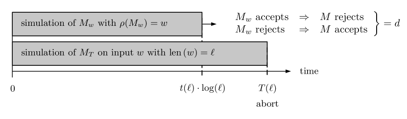
Figure 5: Simulation Setup for the Time Hierarchy Theorem

This changes (9) by rephrasing $L_{D}$ into containing all words for which either of the following two conditions hold:

1. the simulation of $M_{w}$ halts and rejects $w$ within $\leq T(\mathop{\text{len}}\left(w\right))$ steps, provided that $M_{w}$ makes no call to any oracle (i.e., acts as in a non-relativized world),

2. the simulation of $M_{w}^{A}$ halts and accepts $w$ within $\leq T(\mathop{\text{len}}\left(w\right))$ steps (now, there was a call to the oracle, so that the simulation was done for $M_{w}^{A}$ necessarily and the upper additional condition hence inverted the rejection into an acceptance behavior).

Thus, upon relativization using the oracle $A$, the final argument towards proving Theorem 4.6 deteriorate into a humble tautology: $w\in L(M_{w}^{A})$ implies $w\in L_{D}$ and vice versa, so the contradiction that separates $\textsc{Dtime}(t)$ from $\textsc{Dtime}(T)$ can no longer be reached. Observe that this does not mean that the classes are not separated for other reasons, but this particular argument no longer supports that claim. This already suffices to escape relativization, since the so-modified reasoning towards the statement of Theorem 2.4 becomes void in any relativized world where the oracle is actually used. In a non-relativized world, however, there cannot be any call to any oracle, so that condition (51) has no effect whatsoever, and the first of the two above cases will be the only one to apply. Thus, Theorem 4.6 remains to hold and all arguments based upon go unchanged.

What happens in worlds relativized by oracles that separate P from NP? The argument breaks down in exactly the same way as before, and (also as before) we can say nothing about the relation of P and NP then, so no inconsistency arises here either.

These arguments remain intact also for algebrization, if condition (51) is rephrased into speaking about a perhaps necessary “evaluation” of the oracle function. Circuits that lazy-evaluate their logic thus may or may not need their oracle, so that the above condition can be added to our proof with the same semantic and effect as before. Thus, Theorem 2.4’s fundament will generally collapse in algebrized worlds as well.

5.5 Naturalization

Regarding natural proofs, we may ask if a proof of $\textsc{P}\neq\textsc{NP}$ based on Theorem 2.4 is natural? The answer is (again) no! The crucial finding of [15] is that any natural argument lends itself to breaking pseudorandom generators. But in that case, we would also get fast algorithms for some of the very same problems that we wanted to prove hard by showing that $\textsc{P}\neq\textsc{NP}$ [1]. This is the barrier that natural proofs constitute, but starting from Theorem 2.4 lets us bypass this obstacle.

The reason why a natural property $C^{*}$ can be used to break a pseudorandom generator is the disjointness of $C^{*}$ with the image set of some pseudorandom function (constructed from the pseudorandom number generator (PRNG) in a similar style as in [9]), provides a statistical test to distinguish random from pseudorandom (output ensembles). That test employs the poly-time decidability of $C^{*}$ (provided since $C^{*}$ is natural [15]). Weak OWF exist if and only if strong OWF exist [8], so Theorem 2.4 indirectly gives a strong OWF (see [18] or [8, Thm.2.3.2]), which in turn let us construct PRNG whose output cannot be distinguished from uniformly random in polynomial time (see [8, Def.3.3.1, Thm.3.5.12]). This contradiction rules out any statistical test, including the aforementioned one based on deciding $C^{*}$. Hence, in light of Theorem 2.4, a natural property $C^{*}$ cannot exist at all (as is also explicitly said in [15, pg.3]). So, the proof of Corollary 5.1 based on Theorem 2.4 is not natural.

5.6 On the Separation of P from NP

It appears anyway questionable whether we are interested in answering P vs. NP in all possible worlds, rather than under the more realistic assumption of having no particular magic at hand (in the form of an oracle). After all, the question is whether P is equal (or not) to NP, given those (and only those) operations that Turing machines can do. Note that our use of the hierarchy theorem must not be mistakenly interpreted as the high-level claim that $\textsc{P}=\textsc{NP}$ would contradict the hierarchy theorem. The inclusion that we use relates to classes beyond P and hence also above NP under the assumption $\textsc{P}=\textsc{NP}$. So, the hierarchy theorem remains an unshaken base.

Taking Theorem 2.4 as a fundament, we can now complete our discussion by providing the proof of Corollary 5.1 in full detail.

Proof of Corollary 5.1.

Let $f:\Sigma^{*}\to\Sigma^{*}$ be a strong one-way function, whose existence is implied by that of weak one-way functions by [18, Thm.5.2.1]. W.l.o.g., we may assume $\Sigma=\left\{0,1\right\}$ (otherwise, we just use a prefix-free binary encoding to represent all symbols in the finite alphabet $\Sigma$). Moreover, let $gn:\Sigma^{*}\to\mathds{N}$ be a Gödel numbering, for which $gn(w)$ and $gn^{-1}(n)$ are both computable in polynomial time in $\mathop{\text{len}}\left(w\right)$ and $\log(n)$, respectively. Our choice here is the function $gn$ from Section 3.1. We put $g:\mathds{N}\to\mathds{N}$ as $g:=gn\circ f\circ gn^{-1}$, and observe that by (2), $g$ inherits the length regularity property from $f$ (where the integer $n$ has a length $\mathop{\text{len}}\left(n\right)\in\Theta(\log n)$ equal to the number of bits needed to represent it). Furthermore, $g$ is as well strongly one-way: if it were not, i.e., if $g^{-1}(n)$ would be computable in time $\text{poly}(\log n)$, then

$$f^{-1}=gn^{-1}\circ g^{-1}\circ gn$$ (52)

would also be computable in time $\text{poly}(\mathop{\text{len}}\left(w\right))$ (since $gn$ and $gn^{-1}$ are both efficiently computable). Precisely, if some circuit $C$ of $\text{size}(C)\leq\text{poly}(\log n)$ computes $C(n)\in g^{-1}(n)$ with a likelihood of $\geq 1/\text{poly}(\log n)$, then each of these cases is “positive” for the computation of $f^{-1}$ on the entirety of the function’s domain $\left\{0,1\right\}^{\ell}$ with $\ell\in\Theta(\log n)$ (where the $\Theta$ is due to the application of $gn$ and $gn^{-1}$). This means that the circuit $C$ could be extended into a (polynomial size) circuit $C^{\prime}$ that evaluates $f^{-1}$ according to (52) correctly with a likelihood $\geq 1/\text{poly}(\Theta(\ell))$, contradicting the strong one-wayness of $f$.

Upon $g$, we define a language

$$L_{g}:=\left\{(y,N)\in\mathds{N}^{2}:\exists x\in\left\{1,\ldots,N\right\}\text{~{}with~{}}g(x)=y\right\},$$

in which every pair $(y,N)$ can be represented by a word $w\in\left\{0,1\right\}^{\Theta(\log y+\log N)}\in\Sigma^{*}$ using a proper prefix-free encoding (which includes the symbols to separate the binary strings for $y$ and $N$). That is, $L_{g}$ is the set of $y$ for which a preimage within a specified (numeric) range $[1,N]$ exists. Our goal is showing that $L_{g}\in\textsc{NP}$ but $L_{g}\notin\textsc{P}$.

The observation that $L_{g}\in\textsc{NP}$ is immediate, since a preimage $x$ for $y\in\mathds{N}$ has length $O(\log x)$, so it can act as a polynomial witness, guessed by a nondeterministic TM to decide $1\leq x\leq N$ and $g(x)=y$, both doable in time $O(\text{poly}(\log x))$ (as $g$ is length-regular and strongly one-way).

Conversely, if we assume $L_{g}\in\textsc{P}$, then we could efficiently compute $x=g^{-1}(y)$ for every given $y\in\mathds{N}$ by the following method: since $g$ is length regular, it satisfies $\mathop{\text{len}}\left(y\right)=\mathop{\text{len}}\left(g(x)\right)\geq\mathop{\text{len}}\left(x\right)^{1/k}$, where $\mathop{\text{len}}\left(x\right)\in O(\log x)$ when $x$ is treated as a word in binary representation. The value $k$ is a constant that only depends on $g$. Thus, we have the upper bound $\log(x)\in O((\log y)^{k})$, and therefore $x$ lies inside the discrete interval $I=\{1,2,\ldots,N=c\cdot\lceil 2^{(\log y)^{k}}\rceil\}$ for some constant $c>0$ and sufficiently large $x$ (implied by a sufficiently large $y$ via the length-regularity of $g$). With the so-computed $N$, we run a binary search on $I$: per iteration, we can invoke the polynomial-time decision algorithm $A$ available for $L_{g}\in\textsc{P}$ to decide whether to take the left half (if $A$ returns ”yes”) or the right half (if $A$ returns ”no”) of the current search space. After $O(\log N)=O((\log y)^{k})$ iterations, the interval has been narrowed down to contain a single number $x_{0}$, which is the sought preimage of $y$. The whole procedure takes $O((\log y)^{k})\cdot\text{poly}(\log y)$ steps (one decision of $L_{g}$ per iteration of the binary search), and thus is polynomial in $\log y$ since $k$ is a constant. Therefore, $g^{-1}$ would be computable in $O(\text{poly}(\log y))$ steps in the worst case. Since our choice of $y$ was arbitrary, it follows that an evaluation of $g^{-1}$ takes $O(\text{poly}(\log y))$ steps in all cases, which clearly contradicts the average-case hardness of the strong one-way function $g$. Hence, $L_{g}\notin\textsc{P}$, and $\textsc{P}\neq\textsc{NP}$ consequently. ∎

References

- [1] Scott Aaronson and Avi Wigderson. Algebrization: A new barrier in complexity theory. ACM Trans. Comput. Theory, 1(1):2:1–2:54, February 2009.
- [2] Sanjeev Arora and Boaz Barak. Computational Complexity: A Modern Approach. Cambridge University Press, 2009.
- [3] Sanjeev Arora, Russell Impagliazzo, and U. Vazirani. Relativizing versus nonrelativizing techniques: The role of local checkability, 2007. [retrieved: April 20, 2017].
- [4] Theodore Baker, John Gill, and Robert Solovay. Relativizations of the P NP question. SIAM J. Comput., 4(4):431–442, 1975.
- [5] B. Bollobás and A. Thomason. Threshold functions. Combinatorica, 7(1):35–38, 1986.
- [6] Richard Chang, Benny Chor, Oded Goldreich, Juris Hartmanis, Johan Håstad, Desh Ranjan, and Pankaj Rohatgi. The random oracle hypothesis is false. Journal of Computer and System Sciences, 49(1):24–39, 1994.
- [7] Lance Fortnow. The role of relativization in complexity theory. Bulletin of the EATCS, (52):229–244, 1994.
- [8] Oded Goldreich. Foundations of cryptography 1: Basic Tools. Cambridge University Press, 2003.
- [9] Oded Goldreich, Shafi Goldwasser, and Silvio Micali. How to construct random functions. Journal of the ACM, 33(4):792–807, 1986.
- [10] Hans Hermes. Aufzählbarkeit – Entscheidbarkeit – Berechenbarkeit. Springer, 2nd edition, 1971.
- [11] J. E. Hopcroft and J. D. Ullman. Introduction to Automata Theory, Languages and Computation. Addison Wesley, 1979.
- [12] National Institute of Standarts and Technology (NIST). NIST Digital Library of Mathematical Functions, 2023.
- [13] Christos H. Papadimitriou. Computational Complexity. Addison-Wesley, 1994.
- [14] Nicholas Pippenger and Michael J. Fischer. Relations among complexity measures. Journal of the ACM, 26(2):361–381, 1979.
- [15] Alexander A. Razborov and Steven Rudich. Natural proofs. Journal of Computer and System Sciences, 55(1):24–35, 1997.
- [16] M. Sipser. Introduction to the Theory of Computation. PWS Publishing, 3rd edition, 2013.
- [17] Wolfram Research Inc. Mathematica, Version 12.0. 2023.
- [18] Marius Zimand. Compuational Complexity: A Quantitative Approach. North-Holland Mathematical Studies 196. Elsevier, 2004.
- OWF
- one-way function
- TM
- Turing machine
- DTHT
- deterministic time hierarchy theorem
- LCT
- local checkability theorem
- PRNG
- pseudorandom number generator
- ZFC
- Zermelo-Fraenkel set theory with the axiom of choice