Inverse moment problem for non-Abelian Coxeter double Bruhat cells

Abstract.

We solve the inverse problem for non-Abelian Coxeter double Bruhat cells in terms of the matrix Weyl functions. This result can be used to establish complete integrability of the non-Abelian version of nonlinear Coxeter-Toda lattices in $GL_{n}$.

1. Introduction

A fruitful interaction between the operator theory, inverse spectral problems in particular, and the theory of completely integrable systems is, by now, well documented. Beyond just linearizing Hamiltonian equations of interest in mathematical physics, this interaction led to greater insight into geometric properties of underlying objects as well as revealed deep connections with representation theory and algebraic combinatorics.

In one of the first and most famous instances of an interplay between the spectral theory and integrability questions, Moser [32] used a map from finite Jacobi matrices to the space rational functions of fixed degree to linearize the celebrated Toda lattice in the finite non-periodic case. This map associates with a Jacobi matrix a certain matrix element of its resolvent, called the Weyl function. On the other hand, the Atiyah-Hitchin Poisson structure [2] on rational functions initially discovered in the theory of magnetic monopoles, provides a convenient description for the (linear) Hamiltonian structure of the Toda lattice.

In [15]–[17], it was shown that the Atiyah-Hitchin structure belongs to a family of compatible Poisson structures that can be used to establish a multi-Hamiltonian nature of the entire class of ”Toda-like” integrable lattices. In the context of the linear Poisson structure, these lattices are associated with minimal irreducible co-adjoint orbits of the Borel subgroup in $gl_{n}$, while, from the point of view of the quadratic Poisson structure, they are naturally associated with certain class of double Bruhat cells in $GL_{n}$ and belong to the family of so-called Coxeter-Toda lattices. The latter perspective recently led to establishing of a cluster algebra structure in the space of rational functions [26]. Along with Poisson brackets from [16], the key ingredient of this construction was a solution of the inverse problem, that allows to restore the Lax operator of a Coxeter-Toda lattice from its Weyl function in terms of a certain collection of Hankel determinant built from coefficients of the Laurent expansion of the Weyl function. These determinantal formulae generalize the classical ones in the theory of orthogonal polynomials on the real line and on the unit circle.

In this paper, we present an overview of a non-Abelian version of some of the results of [15]–[17] and [26]. Although we will concentrate on finite non-Abelian lattices, it should be pointed out that infinite non-Abelian lattices of Toda type have also attracted a lot of interest of the years. The have been studied in a variety of contexts and via a variety of approaches, using inverse spectral problems in the semi-infinite case [6], [7], inverse scattering in the double-infinite case [9] and methods of algebraic geometry in the periodic case [31].

In the earlier paper [23], we introduce a matrix-valued version of Coxeter-Toda lattices on certain classes of block Hessenberg matrices. These nonlinear lattices generalize both the nonlinear lattices in [15] and the finite non-periodic non-Abelian Toda lattice. We established that a matrix analogue of the Weyl function provides a convenient tool for a study of these non-Abelian Coxeter-Toda lattices. In the case of the non-Abelian Toda lattice, this point of view was advocated in [24]. The lattices of [23] ”live” on noncommutative analogues of elementary Toda orbits – minimal irreducible co-adjoint orbits of the Borel subgroup in $GL_{n}$. In contrast, here we will be more concerned with a noncommutative version of Coxeter double Bruhat cells, whose scalar counterparts are minimal irreducible Poisson submanifolds of $GL_{n}$ equipped with the standard Poisson-Lie structure.

In section 3, we define non-Abelian Coxeter double Bruhat cells, introduce some related combinatorial objects and describe how the elements of non-Abelian Coxeter double Bruhat cells can be parametrized using factorization into elementary factors or, alternatively, using planar directed weighted networks with noncommutative weights. In section 4, the main section of the paper, we presents a solution of the inverse moment problem for non-Abelian Coxeter double Bruhat cells. Here the key role is played by the matrix Weyl function. The main theorem, Theorem 4.2, extends both the results in the commutative case [26] and the partial results obtained in [23]. The factorization parameters are restored as noncommutative monomial expressions in term of Schur complements (quasideterminants) associated with a family of block Hankel matrices built from the coefficients of the Laurent expansion of the matrix Weyl functions. These quasideterminants replace ratios of Hankel determinants needed to express the solution of the inverse problem in the commutative case.

In section 5, we show how this inverse problem combined with the Poisson structure on matrix-valued rational functions introduced earlier in [24] lead to a completely integrable system on every non-Abelian Coxeter double Bruhat cell. We call this system a non-Abelian Coxeter-Toda lattice. The obtained family of integrable lattices incorporates as particular cases all the lattices from [15, 26, 23].

2. Preliminaries

We start by introducing notations and terms to be used throughout the paper. In what follows we will be dealing with block vectors and block matrices whose entries are $m\times m$ matrices. For an $n_{1}\times n_{2}$ block matrix $A=(a_{ij})$, the notation $A^{T}$ will be reserved for its $n_{2}\times n_{1}$ block transpose : $A^{T}=(a_{ji})$.

Denote by $\mathbf{1}_{r}$ the $r\times r$ identity matrix. Sometimes, when the dimension of the identity matrix is clear from context, we will drop the subscript and use $\mathbf{1}$ instead.

Define elementary block vectors $e_{j}=(\delta_{ij}\mathbf{1}_{m})_{i=1}^{n},(j=1,\dots,n)$ and elementary block matrices ${e}_{ij}\otimes\mathbf{1}_{m}=(\delta_{i\alpha}\delta_{j\beta}\mathbf{1}_{m})_{\alpha,\beta=1}^{n}$.

If $P(\lambda)=\sum_{\alpha}\lambda^{\alpha}\pi_{\alpha}$ is a Laurent polynomial with $m\times m$ matrix coefficients, $X$ is an $n\times n$ block matrix and $f$ is a block column vector, we denote by $P(X)f$ the expression $\sum_{\alpha}X^{\alpha}f\pi_{\alpha}$ and by $f^{T}P(X)$ the expression $\sum_{\alpha}\pi_{\alpha}f^{T}X^{\alpha}$.

In what follows, when we deal with an inverse of a block matrix $A=(a_{ij})$, the notation $A_{ij}^{-1}$ is used for an $(i,j)$-block of $A^{-1}$, while $a_{ij}^{-1}$ or $(A_{ij})^{-1}$ will denote the inverse of the $(i,j)$-block of $A$.

Recall that if $A=(a_{ij})_{i,j=1}^{2}$ is a $2\times 2$ block matrix (not necessarily with square blocks) and if a block $A_{ij}$ is square, then its Schur complement is defined as

$$A_{3-i,3-j}^{\square}=A_{3-i,3-j}-A_{3-i,i}(A_{ij})^{-1}A_{j,3-j}\ .$$

Below, we will use the following well-known

Lemma 2.1

Let $G=\left[\begin{array}[]{cc}A&B\\ C&D\end{array}\right]$ be an invertible block matrix, whose block $A$ (resp. $B,C,D$) is square and has an invertible Schur complement. Then $G^{-1}$ is given by the formula

$$G^{-1}=\left[\begin{array}[]{cc}A^{-1}+A^{-1}B(D^{\square})^{-1}CA^{-1}&-A^{-1}B(D^{\square})^{-1}\\ -(D^{\square})^{-1}CA^{-1}&(D^{\square})^{-1}\end{array}\right]\ ,$$ (2.1)

resp.

$$G^{-1}=\left[\begin{array}[]{cc}-C^{-1}D(B^{\square})^{-1}&C^{-1}+C^{-1}D(B^{\square})^{-1}AC^{-1}\\ (B^{\square})^{-1}&-(B^{\square})^{-1}AC^{-1}\end{array}\right]\ ,$$ (2.2)

$$G^{-1}=\left[\begin{array}[]{cc}(A^{\square})^{-1}&-(A^{\square})^{-1}BD^{-1}\\ -D^{-1}C(A^{\square})^{-1}&D^{-1}+D^{-1}C(A^{\square})^{-1}BD^{-1}\end{array}\right]\ ,$$ (2.3)

$$G^{-1}=\left[\begin{array}[]{cc}-(C^{\square})^{-1}DB^{-1}&(C^{\square})^{-1}\\ B^{-1}+B^{-1}A(C^{\square})^{-1}DB^{-1}&-B^{-1}A(C^{\square})^{-1}\end{array}\right]\ .$$ (2.4)

Remark 2.2.

It is easy to see that if the second row of a block matrix $G=\left[\begin{array}[]{cc}A&B\\ C&D\end{array}\right]$ with an invertible square $A$ is a left multiple of the first row, then the Schur complement of $A$ in $G$ is zero.

For $r\in\mathbb{N}$, denote by $[r]$ the set $\{1,\ldots,r\}$. Given an $n_{1}\times n_{2}$ block matrix $A=(a_{ij})$ with $m\times m$ blocks and index sets $I\subset[n_{1}],J\subset[n_{2}]$ we denote by $A_{I}^{J}$ its block submatrix formed by block rows and columns indexed by $i$ and $J$ resp. For $i\in[n_{1}],j\in[n_{2}]$, we denote by $\hat{i},\hat{j}$ their complements in $[n_{1}],[n_{2}]$.

Following [21], we denote by $a_{ij}^{\square}$ the Schur complement of $A_{\hat{i}}^{\hat{j}}$ in $A$ (called a quasideterminant in terminology of [13, 21]) :

$$A_{ij}^{\square}=a_{ij}-A_{i}^{\hat{j}}(A_{\hat{i}}^{\hat{j}})^{-1}A_{\hat{i}}^{j}\ .$$ (2.5)

3. Non-Abelian Coxeter double Bruhat cells

3.1.

In this section, we describe combinatorial notions and parameterizations associated with Coxeter double Bruhat cells adapted to the non-Abelian situation. The discussion here follows that in sect. 3 of [26]. Most of the auxiliary combinatorial statements from that paper can be used without any modifications.

Recall [19] that a double Bruhat cell $G^{u,v}$ in $GL_{n}$ associated with a pair of elements $u,v$ of the permutation group $S_{n}$ is defined as an intersection

$$G^{u,v}=\left({\mathcal{B}}^{+}u{\mathcal{B}}^{+}\right)\cap\left({\mathcal{B}}^{-}v{\mathcal{B}}^{-}\right)\ ,$$ (3.1)

where ${\mathcal{B}}^{\pm}$ denote subgroups of upper and lower triangular invertible matrices in $GL_{n}$ and where $u,v$ are identified with the corresponding permutation matrices $\bar{u},\bar{v}$. Double Bruhat cells in simple and reductive Lie groups where comprehensively studied in [19] in connection with the notion of total positivity. They also served as a chief motivation for defining the notion of cluster algebras, as well as an important example of a class of algebraic varieties supporting a cluster algebra structure [3, 25].

A non-Abelian version of double Bruhat cells was studied in [4]. For our purposes, they can be defined by (3.1) in which ${\mathcal{B}}^{\pm}$ now denote groups of invertible $n\times n$ upper and lower block triangular matrices with $m\times m$ blocks and $u,v$ are now identified with block permutation matrices $\bar{u}\otimes\mathbf{1}_{m},\bar{v}\otimes\mathbf{1}_{m}$.

Factorization of generic elements of $G^{u,v}$ into a product of elementary factors plays an important role in the study of double Bruhat cells in both commutative and noncommutative contexts. For an $m\times m$ matrix $a$ and $i\in[n]$, define elementary block-matrices $E^{+}_{i}(a)$, $E^{-}_{i}(a)$ by

$$E^{+}_{i}(a)=\mathbf{1}_{n}\otimes\mathbf{1}_{m}+e_{i,i+1}\otimes a,\quad E^{-}_{i}(a)=\mathbf{1}_{n}\otimes\mathbf{1}_{m}+e_{i+1,i}\otimes a\ .$$ (3.2)

In other words, $E^{+}_{i}(A)$ (resp. $E^{-}_{i}(A)$) is a block bidiagonal matrix with $\mathbf{1}_{m}$ on the diagonal and the only nonzero off-diagonal block $A$ in a position $(i,i+1)$ (resp. $(i+1,i)$).

As in the scalar case (see, e.g. [18, 19, 20, 26]), it will be convenient to represent block matrices that can be realized as products of elementary ones by planar weighted directed diagrams. In our case, all the weights will be invertible $m\times m$ matrices assigned to edges of the network. Any network $\mathcal{N}$ in question can be drawn in a rectangle, with $n$ sources located on the left side and $n$ sinks on the right side. Both sources and sinks are labeled $1$ to $n$ going from the bottom to the top. All internal vertices are trivalent and are either colored white if it has exactly one incoming edge or black if there are exactly two incoming edges. There are three kinds of edges: horizontal, directed left-to-right and two kinds of inclined edges, directed southwest or northwest. For a directed path $\mathbf{P}$ joining $i$th source with the $j$th sink we define its weight $w({\mathbf{P}})$ as a left-to-right ordered product of egde weights in $w({\mathbf{P}})$. A block matrix $A=A(\mathcal{N})=(a_{ij})_{i,j=1}^{n}$ associated with $\mathcal{N}$ is defined by

$$a_{ij}=\sum_{{\mathbf{P}}:i\rightsquigarrow j}w({\mathbf{P}})\ .$$ (3.3)

For example, a $n\times n$ block diagonal matrix $\operatorname{diag}(d_{1},\ldots,d_{n})$ and elementary block bidiagonal matrices $E^{-}_{i}(l)$ and $E^{+}_{j}(u)$ correspond to planar networks shown in Figure 1 a), b) and c), respectively; all weights not shown explicitly are equal to 1.

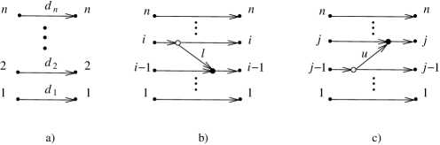
Figure 1. Elementary networks

Two networks of the kind described above can be concatenated by gluing the sinks of the former to the sources of the latter. If $A_{1}$, $A_{2}$ are matrices associated with the two networks, then it is clear that the matrix associated with their concatenation is $A_{1}A_{2}$.

3.2.

Recall that a Coxeter element of $S_{n}$ is any element of length $n-1$ or, in other words, a of all $n-1$ distinct elementary transpositions $s_{i}\ (i=1,\ldots,n-1)$ taken in an arbitrary order. We are only interested in non-Abelian double Bruhat cells associated with a pair of Coxeter elements $u,v$, Coxeter double Bruhat cells for short.

Denote $s_{[p,q]}=s_{p}s_{p+1}\ldots s_{q-1}$ for $1\leq p<q\leq n$ and recall that every Coxeter element $v\in S_{n}$ can be written in the form

$$v=s_{[i_{k-1},i_{k}]}\cdots s_{[i_{1},i_{2}]}s_{[1,i_{1}]}$$ (3.4)

for some subset $I=\{1=i_{0}<i_{1}<\cdots<i_{k}=n\}\subseteq[1,n]$. Besides, define $L=\{1=l_{0}<l_{1}<\cdots<l_{n-k}=n\}$ by $\{l_{1}<\cdots<l_{n-k-1}\}=[1,n]\setminus I$.

Lemma 3.1

Let $v$ be given by (3.4), then

$$v^{-1}=s_{[l_{n-k-1},l_{n-k}]}\cdots s_{[l_{1},l_{2}]}s_{[1,l_{1}]}\ .$$

Let $(u,v)$ be a pair of Coxeter elements and

$$I^{+}= \,\{1=i^{+}_{0}<i^{+}_{1}<\cdots<i^{+}_{k^{+}}=n\},$$ (3.5)

$$I^{-}= \,\{1=i^{-}_{0}<i^{-}_{1}<\cdots<i^{-}_{k^{-}}=n\},$$

$$L^{+}= \,\{1=l^{+}_{0}<l^{+}_{1}<\cdots<l^{+}_{n-k^{+}-1}<l^{+}_{n-k^{+}}=n\},$$

$$L^{-}= \,\{1=l^{-}_{0}<l^{-}_{1}<\cdots<l^{-}_{n-k^{-}-1}<l^{-}_{n-k^{-}}=n\}$$

be subsets of $[1,n]$ that correspond to $v$ and $u^{-1}$ in the way just described.

Certain additional combinatorial data that was utilized in the commutative case [26] can also be employed in a non-Abelian situation. Namely, given a pair $(u,v)$ of Coxeter elements or, equivalently, the sets $I^{\pm}$ given by (3.5), we define, for any $i\in[1,n]$ integers $\varepsilon^{\pm}_{i}$ and $\zeta^{\pm}_{i}$:

$$\varepsilon^{\pm}_{i}=\left\{\begin{array}[]{ll}0,&\mbox{if}\ i=i^{\pm}_{j}\ \mbox{for some}\ 0<j\leq k_{\pm}\,,\\ 1,&\mbox{otherwise}\end{array}\right.$$ (3.6)

and

$$\zeta^{\pm}_{i}=i(1-\varepsilon^{\pm}_{i})-\sum_{\beta=1}^{i-1}\varepsilon^{\pm}_{\beta};$$ (3.7)

note that by definition, $\varepsilon^{\pm}_{1}=1$, $\zeta^{\pm}_{1}=0$. Further, put

$$M^{\pm}_{i}=\{\zeta^{\pm}_{\alpha}\ :\ \alpha=1,\ldots,i\}$$ (3.8)

and

$$k^{\pm}_{i}=\max\{j:i^{\pm}_{j}\leq i\}.$$ (3.9)

Finally, define

$$\varepsilon_{i}=\varepsilon_{i}^{+}+\varepsilon_{i}^{-}$$ (3.10)

and

$$\varkappa_{i}=i+1-\sum_{\beta=1}^{i}\varepsilon_{\beta}.$$ (3.11)

Lemma 3.2

(i) The $n$-tuples $\varepsilon^{\pm}=(\varepsilon^{\pm}_{i})$ and $\zeta^{\pm}=(\zeta^{\pm}_{i})$ uniquely determine each other.

(ii) For any $i\in[1,n]$,

$$\zeta^{\pm}_{i}=\left\{\begin{array}[]{ll}j,&\mbox{if}\ i=i_{j}^{\pm}\ \mbox{for some}\ 0<j\leq k_{\pm}\,,\\ -\sum_{\beta=1}^{i-1}\varepsilon^{\pm}_{\beta},&\mbox{otherwise}.\end{array}\right.$$

(iii) For any $i\in[1,n]$,

$$k^{\pm}_{i}=i-\sum_{\beta=1}^{i}\varepsilon^{\pm}_{\beta},\quad\varkappa_{i}=k_{i}^{+}+k_{i}^{-}-i+1\ .$$

(iv) For any $i\in[1,n]$,

$$M^{\pm}_{i}=[k^{\pm}_{i}-i+1,k^{\pm}_{i}]=\Big{[}1-\sum_{\beta=1}^{i}\varepsilon^{\pm}_{\beta},i-\sum_{\beta=1}^{i}\varepsilon^{\pm}_{\beta}\Big{]}.$$

A set of $m\times m$ complex matrices $c_{1}^{-},\ldots,c_{n-1}^{-};c_{1}^{+},\ldots,c_{n-1}^{+};d_{1},\ldots,d_{n}$ will play a role of noncommutative parameters for generic elements in $G^{u,v}$. We will call $c_{i}^{-}$ lower, $c_{i}^{+}$ upper, and $d_{i}$ diagonal factorization parameters.

Define matrices $D=\operatorname{diag}(d_{1},\ldots,d_{n})$,

$$C^{+}_{j}\!=\!\sum_{\alpha=i^{+}_{j-1}}^{i^{+}_{j}-1}{e}_{\alpha,\alpha+1}\otimes c^{+}_{\alpha},\quad j\in[1,k^{+}],\quad C^{-}_{j}\!=\!\sum_{\alpha=i^{-}_{j-1}}^{i^{-}_{j}-1}{e}_{\alpha+1,\alpha}\otimes c^{-}_{\alpha},\quad j\in[1,k^{-}],$$ (3.12)

and

$$\bar{C}^{+}_{j}\!=\!\sum_{\alpha=l^{+}_{j-1}}^{l^{+}_{j}-1}{e}_{\alpha,\alpha+1}\otimes c^{+}_{\alpha},\quad j\in[1,n-k^{+}],\quad\bar{C}^{-}_{j}\!=\!\sum_{\alpha=l^{-}_{j-1}}^{l^{-}_{j}-1}{e}_{\alpha+1,\alpha}\otimes c^{+}_{\alpha},\quad j\in[1,n-k^{-}].$$

Lemma 3.3

A generic element $X\in G_{m}^{u,v}$ can be written as

$$X=(\mathbf{1}-C^{-}_{1})^{-1}\cdots(\mathbf{1}-C^{-}_{k^{-}})^{-1}D(\mathbf{1}-C^{+}_{k^{+}})^{-1}\cdots(\mathbf{1}-C^{+}_{1})^{-1},$$ (3.13)

and its inverse can be factored as

$$X^{-1}=(\mathbf{1}+\bar{C}^{+}_{n-k^{+}})^{-1}\cdots(\mathbf{1}+\bar{C}^{+}_{1})^{-1}D^{-1}(\mathbf{1}+\bar{C}^{-}_{1})^{-1}\cdots(\mathbf{1}+\bar{C}^{-}_{k^{-}})^{-1}.$$ (3.14)

The network $N_{u,v}$ that corresponds to factorization (3.13) is obtained by the concatenation (left to right) of $2n-1$ building blocks (as depicted in Fig. 1) that correspond to elementary matrices

$$E^{-}_{i^{-}_{2}-1}(c^{-}_{i^{-}_{2}-1}),\ldots,E^{-}_{1}(c^{-}_{1}),E^{-}_{i^{-}_{3}-1}(c^{-}_{i^{-}_{3}-1}),\ldots,E^{-}_{i^{-}_{2}}(c^{-}_{i^{-}_{2}}),\ldots,$$

$$E^{-}_{n-1}(c^{-}_{n-1}),\ldots,E^{-}_{i^{-}_{k^{-}-1}}(c^{-}_{i^{-}_{k^{-}-1}}),D,E^{+}_{i^{+}_{k^{+}-1}}(c^{+}_{i^{+}_{k^{+}-1}}),\ldots,E^{+}_{n-1}(c^{+}_{n-1}),$$

$$\ldots,E^{+}_{i^{+}_{2}}(c^{+}_{i^{+}_{2}}),\ldots E^{+}_{i^{+}_{3}-1}(c^{+}_{i^{+}_{3}-1}),E^{+}_{1}(c^{+}_{1})\cdots E^{+}_{i^{+}_{2}-1}(c^{+}_{i^{+}_{2}-1})\,.$$

This network has $4(n-1)$ internal vertices and $5n-4$ horizontal edges.

Similarly, the network $\bar{N}_{u,v}$ that corresponds to factorization (3.14) is obtained by the concatenation (left to right) of building blocks that correspond to elementary matrices

$$E^{+}_{i^{+}_{2}-1}(-c^{+}_{i^{+}_{2}-1}),\ldots,E^{+}_{1}(-c^{+}_{1}),E^{+}_{i^{+}_{3}-1}(-c^{+}_{i^{+}_{3}-1}),\ldots,E^{+}_{i^{+}_{2}}(-c^{+}_{i^{+}_{2}}),\ldots,$$

$$E^{+}_{n-1}(-c^{+}_{n-1}),\ldots,E^{+}_{i^{+}_{k^{+}-1}}(-c^{+}_{i^{+}_{k^{+}-1}}),D^{-1},E^{-}_{i^{-}_{k^{-}-1}}(-c^{-}_{i^{-}_{k^{-}-1}}),\ldots,E^{-}_{n-1}(-c^{-}_{n-1}),$$

$$\ldots,E^{-}_{i^{-}_{2}}(-c^{-}_{i^{-}_{2}}),\ldots,E^{-}_{i^{-}_{3}-1}(-c^{-}_{i^{-}_{3}-1}),E^{-}_{1}(-c^{-}_{1}),\ldots,E^{-}_{i^{-}_{2}-1}(-c^{-}_{i^{-}_{2}-1})\,.$$

Remark 3.4.

(i) If $v=s_{n-1}\cdots s_{1}$, then $X$ is a block lower Hessenberg matrix, and if $u=s_{1}\cdots s_{n-1}$, then $X$ is a block upper Hessenberg matrix.

(ii) If $v=s_{n-1}\cdots s_{1}$ and $u=s_{1}\cdots s_{n-1}$, then $G^{u,v}$ consists of block tri-diagonal matrices with non-zero off-diagonal entries (block Jacobi matrices). In this case $I^{+}=I^{-}=[1,n]$, $\varepsilon_{1}^{\pm}=1$ and $\varepsilon_{i}^{\pm}=0$ for $i=2,\ldots,n$.

(iii) If $u=v=s_{n-1}\cdots s_{1}$ (which leads to $I^{+}=[1,n],I^{-}=\{1,n\}$), then, in the scalar case, elements of $G^{u,v}$ have a structure of recursion operators arising in the theory of orthogonal polynomials on the unit circle.

(iv) The choice $u=v=(s_{1}s_{3}\cdots)(s_{2}s_{4}\cdots)$ (the so-called bipartite Coxeter element) gives rise to a special kind of pentadiagonal block matrices $X$. In the scalar case, they are called CMV matrices) and serve as an alternative version of recursion operators for orthogonal polynomials on the unit circle [10] and in the complex plane [8].

3.3. Example

Let $n=5$, $v=s_{4}s_{3}s_{1}s_{2}$ and $u=s_{3}s_{2}s_{1}s_{4}$. The network $N_{u,v}$ that corresponds to factorization (3.13) is shown in Figure 2.

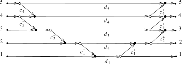
Figure 2. Network representation for elements in $G^{s_{3}s_{2}s_{1}s_{4},s_{4}s_{3}s_{1}s_{2}}$

A generic element $X\in G^{u,v}$ has a form

$$X=(x_{ij})_{i,j=1}^{5}=\left(\begin{array}[]{ccccc}d_{1}&x_{11}c_{1}^{+}&x_{12}c_{2}^{+}&0&0\\ c_{1}^{-}x_{11}&d_{2}+c_{1}^{-}x_{12}&x_{22}c_{2}^{+}&0&0\\ c_{2}^{-}x_{21}&c_{2}^{-}x_{22}&d_{3}+c_{2}^{-}x_{23}&d_{3}c_{3}^{+}&0\\ c_{3}^{-}x_{31}&c_{3}^{-}x_{32}&c_{3}^{-}x_{33}&d_{4}+c_{3}^{-}x_{34}&d_{4}c_{4}^{+}\\ 0&0&0&c_{4}^{-}d_{4}&d_{5}+c_{4}^{-}x_{45}\end{array}\right).$$

One finds by a direct observation that $k^{+}=3$ and $I^{+}=\{i_{0}^{+},i_{1}^{+},i_{2}^{+},i_{3}^{+}\}=\{1,3,4,5\}$, and hence $L^{+}=\{l_{0}^{+},l_{1}^{+},l_{2}^{+}\}=\{1,2,5\}$. Next, $u^{-1}=s_{4}s_{1}s_{2}s_{3}$, therefore, $k^{-}=2$ and $I^{-}=\{i_{0}^{-},i_{1}^{-},i_{2}^{-}\}=\{1,4,5\}$, and hence $L^{-}=\{l_{0}^{-},l_{1}^{-},l_{2}^{-},l_{3}^{-}\}=\{1,2,3,5\}$. Further,

$$\varepsilon^{+}=(1,1,0,0,0),\quad\varepsilon^{-}=(1,1,1,0,0),$$

and hence

$$\zeta^{+}=(0,-1,1,2,3),\quad\zeta^{-}=(0,-1,-2,1,2).$$

Therefore,

$$(k^{+}_{i})_{i=1}^{5}=(0,0,1,2,3),\quad(k^{-}_{i})_{i=1}^{5}=(0,0,0,1,2),$$

and hence

$$(M^{+}_{i})_{i=1}^{5} =([0,0],[-1,0],[-1,1],[-1,2],[-1,3]),$$

$$(M^{-}_{i})_{i=1}^{5} =([0,0],[-1,0],[-2,0],[-2,1],[-2,2]).$$

Finally, $\varepsilon=(2,2,1,0,0)$ and $\varkappa=(0,-1,-1,0,1)$.

The network $\bar{N}_{u^{-1},v^{-1}}$ that corresponds to factorization (3.14) is shown in Figure 3.

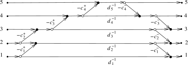
Figure 3. Network $\bar{N}_{u^{-1},v^{-1}}$ for the double Bruhat cell $G^{s_{3}s_{2}s_{1}s_{4},s_{4}s_{3}s_{1}s_{2}}$

4. Inverse problem

4.1.

With each $X\in G^{u,v}$ one associates a matrix Weyl function

$$M(\lambda)=M(\lambda,X)=e_{1}^{T}(\lambda-X)^{-1}e_{1}=\sum_{k=0}^{\infty}\frac{1}{\lambda^{k+1}}h_{k},$$ (4.1)

where

$$h_{k}=e_{1}^{T}X^{k}e_{1}$$ (4.2)

are the moments of $X$.

Our goal is to show how a generic element $X$ of a non-Abelian Coxeter double Bruhat cell $G^{u,v}$ that admits factorization (3.13) can be restored from its Weyl function (4.1) up to a block-diagonal conjugation preserving the Weyl function. We denote by $G^{u,v}/{\mathbf{T}}$ the space of orbits of this action on $G^{u,v}$. Here ${\mathbf{T}}$ denotes the group of invertible block diagonal matrices of the form $T=\operatorname{diag}\left(\mathbf{1}_{m},T_{1},T_{n-1})\right)$.

If $X\in G^{u,v}$ has factorization parameters $c_{i}^{\pm},d_{i}$ and $A$ is a block diagonal matrix $T=\operatorname{diag}\left(\mathbf{1}_{m},c^{-}_{1},\ldots,(c^{-}_{n-1}\cdots c_{1}^{-})\right)$, then $X^{\prime}:=T^{-1}XT$ has all lower parameters equal to $\mathbf{1}_{m}$ and its upper and diagonal parameters are given by

$${\bf c}_{i}=(c^{-}_{i-1}\cdots c_{1}^{-})^{-1}c_{i}^{+}c_{i}^{-}(c^{-}_{i-1}\cdots c_{1}^{-}),\quad{\bf d}_{i}=(c^{-}_{i-1}\cdots c_{1}^{-})^{-1}d_{i}(c^{-}_{i-1}\cdots c_{1}^{-})\ .$$ (4.3)

Clearly, the Weyl function of $X^{\prime}$ coincides with that of $X$ and we can view (4.3) as parameterizing a generic element of $G^{u,v}/{\mathbf{T}}$. In other words, the inverse problem we are interested in solving can be restated as follows: given an element in $X\in G^{u,v}$ with all lower parameters equal to $\mathbf{1}$, restore the remaining factorization parameters ${\bf c}_{i},{\bf d}_{i}$ from the Weyl function $M(\lambda,X)$.

To solve the inverse problem, we combine the approach employed in the commutative situation [17, 26] with the one used in a non-Abelian setting in the block Jacobi case [30, 5] (see also [22, 33]) and block Hessenberg ($v=s_{n-1}\cdots s_{1}$) case [23]. The main idea stems from the classical moments problem [1]: in the commutative case, one considers the space $\mathbb{C}[\lambda,\lambda^{-1}]/\det(\lambda-X)$ equipped with the so-called moment functional - a bi-linear functional $\langle\ ,\ \rangle$ on Laurent polynomials in one variable, uniquely defined by the property

$$\langle\lambda^{i},\lambda^{j}\rangle=h_{i+j}.$$ (4.4)

$X$ is then realized as a matrix of the operator of multiplication by $\lambda$ relative to appropriately selected bases $\{p_{i}^{+}(\lambda)\}_{i=0}^{n-1}$, $\{p_{i}^{-}(\lambda)\}_{i=0}^{n-1}$ bi-orthogonal with respect to the moment functional:

$$\langle p_{i}^{-}(\lambda),p_{j}^{+}(\lambda)\rangle=\delta_{ij}.$$ (4.5)

For example, the classical tridiagonal case corresponds to the orthogonalization of the sequence $1,\lambda,\ldots,\lambda^{n-1}$. Elements of $G^{s_{n-1}\cdots s_{1},s_{n-1}\cdots s_{1}}$ (cf. Remark 3.4(iii)) result from the bi-orthogonalization of sequences $1,\lambda,\ldots,\lambda^{n-1}$ and $\lambda^{-1},\ldots,\lambda^{1-n}$, while CMV matrices (Remark 3.4(iv)) correspond to the bi-orthogonalization of sequences $1,\lambda,\lambda^{-1},\lambda^{2},\ldots$ and $1,\lambda^{-1},\lambda,\lambda^{-2},\ldots$ The non-Abelian case was first treated in pioneering works by M. G. Krein [30] and Yu. M. Berezanskii [5, chapter VII.2] on Jacobi matrices with matrix (operator) valued coefficients. In this case, the moment functional defined by (4.4) becomes a matrix-valued functional that acts on pairs of matrix-valued Laurent polynomials $a(\lambda)=\sum_{i}\lambda^{i}a_{i},b(\lambda)=\sum_{j}^{N}\lambda^{i}b_{j}$ by

$$\langle a(\lambda),b(\lambda\rangle=\sum_{i,j}a_{i}h_{i+j}b_{j}\$$

and, in the tri-diagonal case, coefficients of $X$ are obtained via so-called pseudo-orthogonalization [5] applied to the sequence $\mathbf{1},\lambda\mathbf{1},\ldots$ We will generalize this strategy to the case of arbitrary Coxeter $u,v$.

For any $l\in\mathbb{Z}$, $i\in\mathbb{N}$ define block Hankel matrices

$$\mathcal{H}^{(l)}_{i}=(h_{\alpha+\beta+l-i-1})_{\alpha,\beta=1}^{i}\,.$$ (4.6)

Matrices $\mathcal{H}^{(l)}_{i}$ play the key role in the solution of the inverse problem. Before describing its solution, let us recall the situation in the scalar case which can be summarized in the following theorem quoted from [26].

Theorem 4.1

Let $\Delta_{i}^{(l)}=\det\mathcal{H}^{(l)}_{i}$. If $X\in G^{u,v}$ admits factorization (3.13), then

$${\bf d}_{i}=d_{i} =\frac{\Delta_{i}^{(\varkappa_{i}+1)}\Delta_{i-1}^{(\varkappa_{i-1})}}{\Delta_{i}^{(\varkappa_{i})}\Delta_{i-1}^{(\varkappa_{i-1}+1)}},$$ (4.7)

$${\bf c}_{i}=c_{i}^{+}c_{i}^{-} =\frac{\Delta_{i-1}^{(\varkappa_{i-1})}\Delta_{i+1}^{(\varkappa_{i+1})}}{\left(\Delta_{i}^{(\varkappa_{i}+1)}\right)^{2}}\left(\frac{\Delta_{i+1}^{(\varkappa_{i+1}+1)}}{\Delta_{i+1}^{(\varkappa_{i+1})}}\right)^{\varepsilon_{i+1}}\left(\frac{\Delta_{i-1}^{(\varkappa_{i-1}+1)}}{\Delta_{i-1}^{(\varkappa_{i-1})}}\right)^{2-\varepsilon_{i}}$$

for any $i\in[1,n]$.

The rest of this section is devoted to the proof of the noncommutative analogue of Theorem 4.1 that can be formulated as

Theorem 4.2

If $X$ is a generic element of $G^{u,v}$ admitting factorization (3.13) then corresponding noncommutative factorization parameters ${\bf c}_{i},{\bf d}_{i}$ can be restored as noncommutative monomial expressions in terms of quasideterminants associated with corner block entries of matrices $\mathcal{H}^{(l)}_{i}$.

4.2.

The following short-hand notations will be convenient for us below: for any integers $r<s$ introduce block column vectors $h^{[r,s]}=\mbox{col}[h_{r},h_{r+1},\ldots,h_{s}]$ and a block row vectors $h_{[r,s]}=[h_{r},h_{r+1},\ldots,h_{s}]$. For example, we can partition ${\mathcal{H}}_{i+1}^{(l)}$ as

$${\mathcal{H}}_{i+1}^{(l)} =\left[\begin{array}[]{cc}{\mathcal{H}}_{i}^{(l-1)}&h^{[l,l+i-1]}\\ h_{[l,l+i-1]}&h_{l+i}\end{array}\right]=\left[\begin{array}[]{cc}h_{l-i}&h_{[l-i+1,l]}\\ h^{[l-i+1,l]}&{\mathcal{H}}_{i}^{(l+1)}\end{array}\right]$$ (4.8)

$$=\left[\begin{array}[]{cc}h^{[l-i,l-1]}&{\mathcal{H}}_{i}^{(l)}\\ h_{l}&h_{[l+1,l+i]}\end{array}\right]=\left[\begin{array}[]{cc}h_{[l-i,l-1]}&h_{l}\\ {\mathcal{H}}_{i}^{(l)}&h^{[l+1,l+i]}\end{array}\right]\ .$$

Using (2.5), (4.8) and Lemma 2.1, we can express ”corner” block entries of the inverse of ${\mathcal{H}}_{i+1}^{(l)}$ using quasideterminants:

$$({\mathcal{H}}_{i+1}^{(l)})^{-1}_{11} =\left(({\mathcal{H}}_{i+1}^{(l)})_{11}^{\square}\right)^{-1}\!=\!\left(h_{l-i}-h_{[l-i+1,l]}({\mathcal{H}}_{i}^{(l+1)})^{-1}h^{[l-i+1,l]}\right)^{-1},$$ (4.9)

$$({\mathcal{H}}_{i+1}^{(l)})^{-1}_{1,i+1} =\left(({\mathcal{H}}_{i+1}^{(l)})_{1,i+1}^{\square}\right)^{-1}\!=\!\left(h_{l}-h_{[l-i,l-1]}({\mathcal{H}}_{i}^{(l)})^{-1}h^{[l+1,l+i]}\right)^{-1},$$

$$({\mathcal{H}}_{i+1}^{(l)})^{-1}_{i+1,1} =\left(({\mathcal{H}}_{i+1}^{(l)})_{i+1,1}^{\square}\right)^{-1}\!=\!\left(h_{l}-h_{[l+1,l+i]}({\mathcal{H}}_{i}^{(l)})^{-1}h^{[l-i,l-1]}\right)^{-1},$$

$$({\mathcal{H}}_{i+1}^{(l)})^{-1}_{i+1,i+1} =\left(({\mathcal{H}}_{i+1}^{(l)})_{i+1,i+1}^{\square}\right)^{-1}\!=\!\left(h_{l+i}-h_{[l,l+i-1]}({\mathcal{H}}_{i}^{(l-1)})^{-1}h^{[l,l+i-1]}\right)^{-1}.$$

Note that in the scalar case all expressions above are ratios of Hankel determinants. This is precisely the reason why Theorem 4.2 serves as an noncommutative analogue of Theorem 4.1. Although we are not going to use them below, we should mention the following identities that were proved in [23].

Proposition 4.3

For $k\geq 1$

$$(\mathcal{H}_{k+1}^{(l)})_{k+1,k+1}^{-1}=-(\mathcal{H}_{k+1}^{(l)})_{k+1,1}^{-1}\left((\mathcal{H}_{k}^{(l-1)})_{k,1}^{-1}\right)^{-1}(\mathcal{H}_{k}^{(l)})_{k,k}^{-1}\,,$$ (4.10)

$$(\mathcal{H}_{k+1}^{(l)})_{11}^{-1}=-(\mathcal{H}_{k}^{(l)})_{11}^{-1}\left((\mathcal{H}_{k}^{(l+1)})_{k1}^{-1}\right)^{-1}(\mathcal{H}_{k+1}^{(l)})_{k+1,1}^{-1}\,,$$ (4.11)

$$(\mathcal{H}_{k+1}^{(l)})_{k+1,k+1}^{-1}\big{(}(\mathcal{H}_{k+1}^{(l)})_{1,k+1}^{-1}\big{)}^{-1}=-(\mathcal{H}_{k}^{(l)})_{kk}^{-1}\big{(}(\mathcal{H}_{k}^{(l-1)})_{1k}^{-1}\big{)}^{-1}\,.$$ (4.12)

Next, we will use relations between moments (4.2) to define a matrix analogue of the characteristic polynomial for $X$.

Lemma 4.4

For a generic $X\in\mathcal{H}$, the Weyl function can be factored as

$$M(\lambda)=Q(\lambda)P^{-1}(\lambda)\ ,$$ (4.13)

where $P(\lambda),Q(\lambda)$ are monic matrix polynomials with $n\times n$ matrix coefficients of degrees $n,n-1$ resp. In particular,

$$P(\lambda)=\lambda^{n}\mathbf{1}-\lambda^{n-1}F_{n-1}-\cdots-F_{0}\ .$$

Proof.

Equation (4.13) is equivalent to relations

$$h_{k+n}=\sum_{j=0}^{n-1}h_{k+j}F_{j}\quad(k=0,1,\ldots)\,,$$ (4.14)

which, in turn, can be re-written as

$$\mathcal{H}^{(l+1)}_{n}=\mathcal{H}^{(l)}_{n}\left[\begin{array}[]{cccc}0&&\cdots&F_{0}\\ \mathbf{1}&\ddots&&\vdots\\ &\ddots&&\\ &&\mathbf{1}&F_{n-1}\end{array}\right]$$ (4.15)

for all $l\in\mathbb{Z}$. The latter follows from (4.6) and the fact that, for a generic $X$, block column $X^{n}e_{1}$ is a linear combination over $gl_{m}$ of block columns $e_{1},Xe_{1},\ldots,X^{n-1}e_{1}$: $X^{n}e_{1}=e_{1}F_{0}+\cdots+X^{n-1}e_{1}F_{n-1}$. ∎

Remark 4.5.

It is a corollary of the proof above that $X$ is similar to the block companion matrix that appears in the right hand side of (4.15). This means, in particular that the characteristic polynomial of $X$ coincides with $\det P(\lambda)$.

If $u,v,\ldots$ are block row or column vectors, we will denote by ${\operatorname{span}}_{gl_{m}}\{u,v,\ldots\}$ the space of all combinations of $A_{u}u+A_{v}v+\cdots$ with $m\times m$ matrix coefficients $A_{u},A_{v},\ldots$ For any $i\in[n]$ define subspaces

$${\mathcal{L}}^{+}_{i}={\operatorname{span}}_{gl_{m}}\{e^{T}_{1},\dots,e^{T}_{i}\},\quad{\mathcal{L}}^{-}_{i}={\operatorname{span}}_{gl_{m}}\{e_{1},\ldots,e_{i}\}.$$

Let

$${\displaystyle{\bf{\bf\gamma}}^{+}_{i}=\begin{cases}\vec{\prod}_{\beta=0}^{j-1}\left({\mathbf{d}}_{i^{+}_{\beta}}{\mathbf{c}}_{i_{\beta}^{+}}\cdots{\mathbf{c}}_{i^{+}_{\beta+1}-1}\right)\,,&\mbox{if }i=i_{j}^{+}\,,\\ (-1)^{l^{+}_{\alpha}-1}\vec{\prod}_{\beta=0}^{\alpha-1}\left({\mathbf{c}}_{l^{+}_{\beta}}\cdots{\mathbf{c}}_{l^{+}_{\beta+1}-1}{\mathbf{d}}^{-1}_{l^{+}_{\beta}+1}\right)\,,&\mbox{if }i=l_{\alpha}^{+}\,,\end{cases}}$$ (4.16)

$${\displaystyle{\bf{\bf\gamma}}^{-}_{i}=\begin{cases}{\mathbf{d}}_{i^{-}_{j-1}}\cdots{\mathbf{d}}_{i^{-}_{0}}\,,&\mbox{if }i=i_{j}^{-}\,,\\ (-1)^{l^{-}_{\alpha}-1}{\mathbf{d}}^{-1}_{l^{-}_{\alpha}}\cdots{\mathbf{d}}^{-1}_{l^{-}_{1}}\,,&\mbox{if }i=l_{\alpha}^{-},\ i<n\,,\end{cases}}$$ (4.17)

where $i^{\pm}_{j},l^{\pm}_{\alpha}$ are defined in (3.5) and ${\bf{\bf\gamma}}^{\pm}_{1}=1$  .

Remark 4.6.

Note an expression for ${\bf{\bf\gamma}}_{i}^{+}$ has a form ${\bf{\bf\gamma}}_{i}^{+}=\mu\ {\mathbf{c}}_{i-1}$ if $\varepsilon_{i}^{+}=0$ or ${\bf{\bf\gamma}}_{i}^{+}=\mu\ {\mathbf{c}}_{i-1}{\mathbf{d}}_{i}^{-1}$ if $\varepsilon_{i}^{+}=1$, where in both cases $\mu$ is a noncommutative monomial in ${\mathbf{c}}_{\alpha}\ (\alpha<i-1)$ and ${\mathbf{d}}^{\pm 1}_{\beta}\ (\beta<i)$. This means, in particular, that all weights ${\mathbf{c}}_{1},\ldots,{\mathbf{c}}_{n-1}$ can be uniquely restored from ${\mathbf{d}}_{1},\ldots,{\mathbf{d}}_{n}$ and ${\bf{\bf\gamma}}_{1}^{+},\ldots,{\bf\gamma}_{n}^{+}$ as noncommutative monomial expressions.

Lemma 4.7

For any $i\in[1,n]$ one has

$$e^{T}_{1}X^{\zeta^{+}_{i}}={\bf\gamma}^{+}_{i}e^{T}_{i}\mod{\mathcal{L}}^{+}_{i-1}$$ (4.18)

and

$$X^{\zeta^{-}_{i}}e_{1}=e_{i}{\bf\gamma}^{-}_{i}\mod{\mathcal{L}}^{-}_{i-1}.$$ (4.19)

In particular,

$${\mathcal{L}}^{+}_{i}={\operatorname{span}}_{gl_{m}}\{e^{T}_{1}X^{\zeta^{+}_{1}},\dots,e^{T}_{1}X^{\zeta^{+}_{i}}\},\quad{\mathcal{L}}^{-}_{i}={\operatorname{span}}_{gl_{m}}\{X^{\zeta^{-}_{1}}e_{1},\dots,X^{\zeta^{-}_{i}}e_{1}\}.$$

In addition,

$$X^{\zeta^{-}_{n}-n}e_{1}=(-1)^{n-1}e_{n}\left({\mathbf{d}}^{-1}_{n}{\mathbf{d}}^{-1}_{l^{-}_{n-k^{-}-1}}\cdots{\mathbf{d}}^{-1}_{l^{-}_{1}}\right):=(-1)^{n-1}e_{n}\tilde{\mathbf{\gamma}}_{n}\mod{\mathcal{L}}^{-}_{n-1}.$$ (4.20)

Proof.

The proof given in [26] relies only on the combinatorics of networks associated with $X,X^{-1}$ and thus can be applied to the noncommutative case as well. The idea is that to analyze $X^{k}e_{1}$ (resp. $e_{1}^{T}X^{k}$) for some $k\in\mathbb{Z}$ , one can consider a network obtained by concatenation of $|k|$ copies of the network that corresponds to $X^{\mbox{sign}k}$ and find what is the highest horizontal level that can be reached by a path starting at the lowest level on the right (resp. on the left). The upshot is that if $k=\zeta_{i}^{-}$ (resp. $k=\zeta_{i}^{+}$) then the level is given by $i$ and the corresponding path is unique. The weight of this path is equal to ${\bf\gamma}_{i}^{-}$ (resp. ${\bf\gamma}_{i}^{+}$). ∎

Example 4.8.

We illustrate (4.18) using Example 3.3 and Fig. 2. If $j>0$ then to find $i$ such that $e_{1}^{T}X^{j}={\bf\gamma}^{+}_{i}e^{T}_{i}\mod{\mathcal{L}}^{+}_{i-1}$ it is enough to find the highest sink that can be reached by a path starting from the source 1 in the network obtained by concatenation of $j$ copies of $N_{u,v}$. Thus, we conclude from Fig. 2, that

$$e_{1}^{T}X =d_{1}c_{1}^{+}c_{2}^{+}e^{T}_{3}\mod{\mathcal{L}}^{+}_{2},\quad e_{1}^{T}X^{2}=d_{1}c_{1}^{+}c_{2}^{+}d_{3}c_{3}^{+}e^{T}_{4}\mod{\mathcal{L}}^{+}_{3},$$

$$e_{1}^{T}X^{3} =d_{1}c_{1}^{+}c_{2}^{+}d_{3}c_{3}^{+}d_{4}c_{4}^{+}e^{T}_{5}\mod{\mathcal{L}}^{+}_{4}.$$

Similarly, using the network $\bar{N}_{u^{-1},v^{-1}}$ shown in Fig. 3, one observes that $e_{1}^{T}X^{-1}=-c_{1}^{+}d_{2}^{-1}e^{T}_{2}\mod{\mathcal{L}}^{+}_{1}$. These relations are in agreement with (4.18).

Lemma 4.9

The matrix $F_{0}$ in (4.14) has an expression

$$F_{0}=(-1)^{n-1}{\mathbf{d}}_{l^{-}_{1}}\cdots{\mathbf{d}}_{l^{-}_{n-k^{-}-1}}{\mathbf{d}}_{n}{\mathbf{d}}_{i^{-}_{k^{-}-1}}\cdots{\mathbf{d}}_{i^{-}_{1}}{\mathbf{d}}_{1}\ .$$

Proof.

Multiplying the equation $X^{n}e_{1}=e_{1}F_{0}+\cdots+X^{n-1}e_{1}F_{n-1}$ on the left by $X^{\zeta^{-}_{n}-n}$ we obtain

$$X^{\zeta^{-}_{n}}e_{1}=X^{\zeta^{-}_{n}-n}e_{1}F_{0}+\cdots+X^{\zeta^{-}_{n}-1}e_{1}F_{n-1}\ .$$

From definitions (3.6)–(3.11) and Lemma 3.2 we conclude that $M_{n-1}^{-}=\{\zeta^{-}_{\alpha}\ :\ \alpha=1,\ldots,n-1\}=\left[\zeta^{-}_{n}-n+1,\zeta^{-}_{n}-1\right]$. By Lemma 4.7, this means that in the equality above only the left hand side and the first term in the right hand side have non-zero last block entries, equal to ${\bf\gamma}^{-}_{n}$ and $(-1)^{n-1}\tilde{\bf\gamma}^{-}_{n}F_{0}$, resp. Therefore, $F_{0}=(-1)^{n-1}\left(\tilde{\bf\gamma}^{-}_{n}\right)^{-1}{\bf\gamma}^{-}_{n}$, which proves the claim. ∎

Lemma 4.10

Let $k\in[1,n-1]$ and $X_{i}$ be the $k\times k$ block submatrix of $X\in G^{u,v}$ obtained by deleting $n-k$ last block rows and columns. Then

$$h_{\alpha}(X_{k})=h_{\alpha}(X)$$ (4.21)

for $\alpha\in[\varkappa_{k}-k+1,\varkappa_{k}+k]$.

Proof.

The proof in the scalar case was given in [26]. It depends only on combinatorics of networks $N_{u,v}$ and $\bar{N}_{u^{-1},v^{-1}}$ and thus translates to the non-Abelian case without any changes. ∎

4.3.

The solution of the inverse problem relies on properties of matrix polynomials of the form

$${{\mathcal{\mathbf{P}}}}^{(l)}_{i}(\lambda) =\left[\begin{array}[]{cccc}h_{l-i+1}&h_{l-i+2}&\cdots&h_{l+1}\\ \cdots&\cdots&\cdots&\cdots\\ h_{l}&h_{l+1}&\cdots&h_{l+i}\\ \mathbf{1}&\lambda\mathbf{1}&\cdots&\lambda^{i}\mathbf{1}\end{array}\right]_{i+1,i+1}^{\square}$$

$$=\lambda^{i}-\left[\mathbf{1}\ \lambda\mathbf{1}\ \cdots\lambda^{i-1}\mathbf{1}\right]\left(\mathcal{H}^{(l)}_{i}\right)^{-1}h^{[l+1,l+i]}.$$

Lemma 4.11

Expand ${\mathcal{\mathbf{P}}}^{(l)}_{i}(\lambda)$ as ${\mathcal{\mathbf{P}}}^{(l)}_{i}(\lambda)=\sum_{\alpha=0}^{i}\lambda^{i}\pi_{\alpha}$. Then

$$e_{1}^{T}X^{\beta}{\mathcal{\mathbf{P}}}^{(l)}_{i}(X)e_{1}= \sum_{\alpha=0}^{i}h_{\alpha+\beta}\pi_{\alpha}=0\ \quad\mbox{for}\quad\beta\in[l-i,l-1],$$ (4.27)

$$e_{1}^{T}X^{l+1}{\mathcal{\mathbf{P}}}^{(l)}_{i}(X)e_{1}= \sum_{\alpha=0}^{i}h_{\alpha+l+1}\pi_{\alpha}=\left(\mathcal{H}^{(l+1)}_{i+1}\right)^{\square}_{i+1,i+1}\ ,$$

$$e_{1}^{T}X^{l-i}{\mathcal{\mathbf{P}}}^{(l)}_{i}(X)e_{1}= \sum_{\alpha=0}^{i}h_{\alpha+l-i}\pi_{\alpha}=\left(\mathcal{H}^{(l)}_{i+1}\right)^{\square}_{1,i+1}\ .$$

Proof.

The first equality in all three lines follows from (4.3) and (4.2). It is easy to see that, for $\beta\in[l-i,l-1]$, $\sum_{\alpha=0}^{i}h_{\alpha+\beta}\pi_{\alpha}$ is equal to the $(i+1,i+1)$-quasideterminant of the block matrix obtained from $\mathcal{H}^{(l+1)}_{i+1}$ by replacing the last block row with the block row number $\beta+i-l$. By Remark 2.2, this quasideterminant is equal to zero. This prove the first equality in this Lemma. The other two follow from (4.3) combined with (4.9). ∎

Corollary 4.12

Let ${\mathcal{\mathbf{P}}}(\lambda)$ be the matrix polynomial defined in Lemma 4.4. Then, for any $l\in\mathbb{Z}$,

$${\mathcal{\mathbf{P}}}(\lambda)={\mathcal{\mathbf{P}}}^{(l)}_{n}(\lambda)\ .$$

Proof.

The claim follows from comparing (4.14) with the first equation in Lemma 4.27. ∎

Lemma 4.13

$${\mathcal{\mathbf{P}}}^{(l)}_{i}(0)=-({\mathcal{H}}_{i}^{(l)})^{-1}_{11}\left(({\mathcal{H}}_{i}^{(l+1)})^{-1}_{1i}\right)^{-1}=-\left(({\mathcal{H}}_{i}^{(l)})^{\square}_{11}\right)^{-1}({\mathcal{H}}_{i}^{(l+1)})^{\square}_{1i}\ .$$

Proof.

By (4.3), ${\mathcal{\mathbf{P}}}^{(l)}_{i}(0)=-\left[\mathbf{1}\ 0\ \cdots\ 0\right]\left(\mathcal{H}^{(l)}_{i}\right)^{-1}h^{[l+1,l+i]}$. Using (2.3), the latter expression can be rewritten as $-({\mathcal{H}}_{i}^{(l)})^{-1}_{11}\left(h_{l+1}-h_{[l-i+1,l]}({\mathcal{H}}_{i-1}^{(l+1)})^{-1}h^{[l+2,l+i]}\right)$, which proves the claim when one takes into consideration the second equality in (4.9). ∎

Lemma 4.14

For $k\in[1,n]$,

$${\mathcal{\mathbf{P}}}^{(\varkappa_{k})}_{k}(0)=(-1)^{k-1}\left(\overrightarrow{\prod}_{1<l^{-}_{\alpha}<k}{\mathbf{d}}_{l^{-}_{\alpha}}\right){\mathbf{d}}_{k}\left(\overleftarrow{\prod}_{1\leq i^{-}_{\beta}<k}{\mathbf{d}}_{i^{-}_{\beta}}\right)\,.$$

Proof.

Consider the matrix $X_{k}$ as defined in Lemma 4.21. Since $h_{\alpha}(X_{k})=h_{\alpha}(X)$ for $\alpha\in[\varkappa_{k}-k+1,\varkappa_{k}+k]$, $k\times k$ block Hankel matrices ${\mathcal{H}}_{k}^{(\varkappa_{k})}$ and ${\mathcal{H}}_{k}^{(\varkappa_{k}+1)}$ can be chosen to play the same role for $X_{k}$ that $n\times n$ block Hankel matrices ${\mathcal{H}}_{n}^{(l)}$ and ${\mathcal{H}}_{n}^{(l+1)}$ play in the equation (4.15) for $X$. By Corollay 4.12 this implies, in turn, that matrix polynomial ${\mathcal{\mathbf{P}}}^{(\varkappa_{k})}_{k}(\lambda)$ plays the same role for $X_{k}$ that ${\mathcal{\mathbf{P}}}^{(l)}_{n}(\lambda)$ does for $X$. In particular, we can apply Lemma 4.9 to express ${\mathcal{\mathbf{P}}}^{(\varkappa_{k})}_{k}(0)$ using diagonal weights of $X_{k}$ which coincide with the first $k$ diagonal weights of $X$. The claim then follows from Lemma 4.9. ∎

Proposition 4.15

Define matrix Laurent polynomials

$${\bf p}_{i}(\lambda)=(-1)^{(i-1)\varepsilon_{i}^{-}}\lambda^{k^{-}_{i}-i+1}{\mathcal{\mathbf{P}}}^{(\varkappa_{i-1}-\varepsilon_{i}^{-})}_{i-1}(\lambda)\left({\mathcal{\mathbf{P}}}^{(\varkappa_{i-1}-\varepsilon_{i}^{-})}_{i-1}(0)\right)^{-\varepsilon_{i}^{-}}({\bf\gamma}_{i}^{-})^{-1},\quad i\in[1,n].$$

Then

$${\bf p}_{i}(X)e_{1}=e_{i},\quad i\in[1,n].$$

Proof.

Expand ${\mathcal{\mathbf{P}}}^{(\varkappa_{i-1}-\varepsilon_{i}^{-})}_{i-1}(\lambda)$ as ${\mathcal{\mathbf{P}}}^{(\varkappa_{i-1}-\varepsilon_{i}^{-})}_{i-1}(\lambda)=\sum_{\alpha=0}^{i-1}\lambda^{\alpha}\pi_{\alpha}$. Then Lemma 4.27 implies that

$$\sum_{\alpha=0}^{i-1}h_{\alpha+\beta}\pi_{\alpha}=0$$ (4.28)

for $\beta\in[\varkappa_{i-1}-\varepsilon_{i}^{-}-i+1,\varkappa_{i-1}-\varepsilon_{i}^{-}-1]$.

It follows from Lemma 4.7 that

$$e_{i}{\bf\gamma}_{i}^{-}=X^{\zeta_{i}^{-}}e_{1}+\sum_{\alpha=1}^{i-1}X^{\zeta^{-}_{\alpha}}e_{1}\zeta_{\alpha}$$

for some $m\times m$ coefficients $\zeta_{\alpha}$. By Lemma 3.2(iv), this can be re-written as

$$e_{i}{\bf\gamma}_{i}^{-}=X^{k^{-}_{i}-i+1}\sum_{\alpha=0}^{i-1}X^{\alpha-1}e_{1}\tilde{\pi}_{\alpha},$$ (4.29)

where either $\tilde{\pi}_{i-1}=1$ (if $\varepsilon_{i}^{-}=0$), or $\tilde{\pi}_{0}=1$ (if $\varepsilon_{i}^{-}=1$). Define a matrix polynomial ${\bf p}(\lambda)=\sum_{\alpha=0}^{i-1}\lambda^{\alpha}\tilde{\pi}_{\alpha}$. By Lemma 4.7, block vectors $e_{1}^{T}X^{\beta}$, $\beta\in M^{+}_{i-1}$, span ${\mathcal{L}}^{+}_{i-1}$ over $gl_{m}$. Therefore, by Lemma 3.2(iv),

$$0=e_{1}^{T}X^{\beta}X^{k^{-}_{i}-i+1}{\bf p}(X)e_{1}=\sum_{\alpha=0}^{i-1}h_{\alpha+\beta+k^{-}_{i}-i+1}\tilde{\pi}_{\alpha}$$ (4.30)

for $\beta\in[k_{i-1}^{+}-i+2,k_{i-1}^{+}]$. Using Lemma 3.2 (iii), we conclude that $k^{-}_{i}=k^{-}_{i-1}+1-\varepsilon^{-}_{i}$ and that in the equation (4.29) $(\beta+k^{-}_{i}-i+1)$ ranges through the interval $\beta\in[\varkappa_{i-1}-\varepsilon_{i}^{-}-i+1,\varkappa_{i-1}-\varepsilon_{i}^{-}-1]$.

Comparing with (4.30), we see that coefficients of polynomials ${\bf p}(\lambda)$ and ${\mathcal{\mathbf{P}}}^{(\varkappa_{i-1}-\varepsilon_{i}^{-})}_{i-1}(\lambda)$ satisfy the same system of linear equations. The genericity assumption guarantees that this system has a unique solution if one requires that either the leading or degree zero coefficient of the resulting polynomial is equal to $\mathbf{1}$. Indeed, the unique solvability of the system in this case relies on invertibility of the block Hankel matrices $\mathcal{H}^{(l-1)}_{i-1}$, $\mathcal{H}^{(l)}_{i-1}$ resp., where $l=\varkappa_{i-1}-\varepsilon_{i}^{-}$. This means that ${\bf p}(\lambda)={\mathcal{\mathbf{P}}}^{(\varkappa_{i-1}-\varepsilon_{i}^{-})}_{i-1}(\lambda)$ if $\varepsilon_{i}^{-}=0$ and ${\bf p}(\lambda)={\mathcal{\mathbf{P}}}^{(\varkappa_{i-1}-\varepsilon_{i}^{-})}_{i-1}(\lambda)\pi_{0}^{-1}$ otherwise. Then it drops out from (4.29) that

$$e_{i}=X^{k^{-}_{i}-i+1}{\mathcal{\mathbf{P}}}^{(\varkappa_{i-1}-\varepsilon_{i}^{-})}_{i-1}(X)e_{1}\pi_{0}^{-\varepsilon_{i}^{-}}({\bf\gamma}_{i}^{-})^{-1}\ ,$$

which proves the claim. ∎

4.4.

Finally, we can complete the proof of Theorem 4.2. Lemma 4.13 and Lemma 4.14 imply the equation

$${\mathbf{d}}_{k}=(-1)^{k}\left(\overrightarrow{\prod}_{1<l^{-}_{\alpha}<k}{\mathbf{d}}_{l^{-}_{\alpha}}\right)^{-1}\left(({\mathcal{H}}_{k}^{(\varkappa_{k})})^{\square}_{11}\right)^{-1}({\mathcal{H}}_{k}^{(\varkappa_{k}+1)})^{\square}_{1k}\left(\overleftarrow{\prod}_{1\leq i^{-}_{\beta}<k}{\mathbf{d}}_{i^{-}_{\beta}}\right)^{-1}\ ,$$

which allows to recursively restore $d_{1},\ldots,d_{n}$ as noncommutative monomials in terms of corner quasideterminants of block Hankel matrices ${\mathcal{H}}_{k}^{(\varkappa_{k})},{\mathcal{H}}_{k}^{(\varkappa_{k}+1)}$.

Next, observe that by Lemma 4.7 and Corollary 4.15,

$$\begin{split}{\bf{\bf\gamma}}_{i}^{+}&=e_{1}^{T}X^{\zeta_{i}^{+}}{\bf p}_{i}(X)e_{1}\\ &=(-1)^{(i-1)\varepsilon_{i}^{-}}\left(e_{1}^{T}X^{\zeta_{i}^{+}+k^{-}_{i}-i+1}{\mathcal{\mathbf{P}}}^{(\varkappa_{i-1}-\varepsilon_{i}^{-})}_{i-1}(X)e_{1}\right)\left({\mathcal{\mathbf{P}}}^{(\varkappa_{i-1}-\varepsilon_{i}^{-})}_{i-1}(0)\right)^{-\varepsilon_{i}^{-}}({\bf{\bf\gamma}}_{i}^{-})^{-1}.\end{split}$$

Since by (3.7), (3.10), (3.11) and Lemma 3.2(iii),

$$\zeta_{i}^{+}+k_{i}^{-}-i+1=\varkappa_{i}-(i-1)\varepsilon_{i}^{+}\ =\begin{cases}\varkappa_{i-1}-\varepsilon_{i}^{-}+1,&\mbox{if}\quad\varepsilon_{i}^{+}=0\,,\\ \varkappa_{i-1}-\varepsilon_{i}^{-}-i+1,&\mbox{if}\quad\varepsilon_{i}^{+}=1\,,\end{cases}$$

we can apply the second (if $\varepsilon_{i}^{+}=0$) or the third (if $\varepsilon_{i}^{+}=1$) equality in Lemma 4.27 with $i$ replaced with $i-1$ and $l=\varkappa_{i}-1$ to conclude that

$$e_{1}^{T}X^{\zeta_{i}^{+}+k^{-}_{i}-i+1}{\mathcal{\mathbf{P}}}^{(\varkappa_{i-1}-\varepsilon_{i}^{-})}_{i-1}(X)e_{1}=\begin{cases}\left(\mathcal{H}^{(\varkappa_{i})}_{i}\right)^{\square}_{ii},&\mbox{if}\quad\varepsilon_{i}^{+}=0\,,\\ \ &\\ \left(\mathcal{H}^{(\varkappa_{i})}_{i}\right)^{\square}_{1i},&\mbox{if}\quad\varepsilon_{i}^{+}=1\,.\end{cases}$$

Thus

$${\bf{\bf\gamma}}_{i}^{+}{\bf{\bf\gamma}}_{i}^{-}=-(-1)^{(i-1)\varepsilon_{i}^{-}}\left(\mathcal{H}^{(\varkappa_{i})}_{i}\right)^{\square}_{i-(i-1)\varepsilon_{i}^{+},i}\left(\left(({\mathcal{H}}_{i}^{(\varkappa_{i-1}-\varepsilon_{i}^{-})})^{\square}_{11}\right)^{-1}({\mathcal{H}}_{i}^{(\varkappa_{i-1}-\varepsilon_{i}^{-}+1)})^{\square}_{1i}\right)^{-\varepsilon_{i}^{-}}\,.$$

This relation, together with Remark 4.6, completes the proof of Theorem 4.2.

5. Non-Abelian Coxeter-Toda lattices

5.1.

We start this section by reviewing basic facts about Toda flows on $GL_{n}$. These are commuting Hamiltonian flows generated by conjugation-invariant functions on $GL_{n}$ with respect to the standard Poisson–Lie structure. Toda flows (also known as characteristic Hamiltonian systems) are defined for an arbitrary standard semi-simple Poisson–Lie group, but we will concentrate on the $GL_{n}$ case, where as a maximal algebraically independent family of conjugation-invariant functions one can choose $F_{k}:GL_{n}\ni X\mapsto\frac{1}{k}\operatorname{tr}X^{k}$, $k=1,\ldots,n-1$. The equation of motion generated by $F_{k}$ has a Lax form

$$dX/dt=\left[X,\ -\frac{1}{2}\left(\pi_{+}(X^{k})-\pi_{-}(X^{k})\right)\right],$$ (5.1)

where $\pi_{+}(A)$ and $\pi_{-}(A)$ denote strictly upper and lower parts of a matrix $A$.

Any double Bruhat cell $G^{u,v}$, $u,v\in S_{n}$, is a regular Poisson submanifold in $GL_{n}$ invariant under the right and left multiplication by elements of the maximal torus (the subgroup of diagonal matrices) ${\mathcal{T}}\subset GL_{n}$. In particular, $G^{u,v}$ is invariant under the conjugation by elements of ${\mathcal{T}}$. The standard Poisson–Lie structure is also invariant under the conjugation action of ${\mathcal{T}}$ on $GL_{n}$. This means that Toda flows defined by (5.1) induce commuting Hamiltonian flows on $G^{u,v}/{\mathcal{T}}$ where ${\mathcal{T}}$ acts on $G^{u,v}$ by conjugation. In the case when $v=u^{-1}=(n\ 1\ 2\ldots n-1)$, $G^{u,v}$ consists of tridiagonal matrices with nonzero off-diagonal entries, $G^{u,v}/\mathcal{H}$ can be conveniently described as the set ${\operatorname{Jac}}$ of Jacobi matrices of the form

$$L=\left(\begin{array}[]{ccccc}b_{1}&a_{1}&0&\cdots&0\\ 1&b_{2}&a_{2}&\cdots&0\\ &\ddots&\ddots&\ddots&\\ &&&b_{n-1}&a_{n-1}\\ 0&&&1&b_{n}\end{array}\right),\quad a_{1}\cdots a_{n-1}\neq 0,\quad\det L\neq 0.$$

Lax equations (5.1) then become the equations of the finite nonperiodic Toda hierarchy

$$dL/dt=[L,-\pi_{+}(L^{k})],$$

the first of which, corresponding to $k=1$, is the celebrated Toda lattice

$$da_{j}/dt = a_{j}(b_{j+1}-b_{j}),\quad j=1,\ldots,n-1,$$

$$db_{j}/dt = (a_{j}-a_{j-1}),\quad j=1,\ldots,n,$$

with the boundary conditions $a_{0}=a_{n}=0$. Recall that $\det L$ is a Casimir function for the standard Poisson–Lie bracket. The level sets of the function $\det L$ foliate ${\operatorname{Jac}}$ into $2(n-1)$-dimensional symplectic manifolds, and the Toda hierarchy defines a completely integrable system on every symplectic leaf. Note that although Toda flows on an arbitrary double Bruhat cell $G^{u,v}$ can be exactly solved via the so-called factorization method, in most cases the dimension of symplectic leaves in $G^{u,v}/{\mathcal{T}}$ exceeds $2(n-1)$, which means that conjugation-invariant functions do not form a Poisson commuting family rich enough to ensure Liouville complete integrability.

An important role in the study of Toda flows played by the Weyl function

$$m(\lambda)=m(\lambda;X)=((\lambda\mathbf{1}-X)^{-1}e_{1},e_{1})=\frac{q(\lambda)}{p(\lambda)},$$ (5.2)

in the scalar case is well-known. Here $p(\lambda)$ is the characteristic polynomial of $x$ and $q(\lambda)$ is the characteristic polynomial of the $(n-1)\times(n-1)$ submatrix of $x$ formed by deleting the first row and column. Differential equations that describe the evolution of $m(\lambda;X)$ induced by Toda flows do not depend on the initial value $x(0)$ and are easy to solve: though nonlinear, they are also induced by linear differential equations with constant coefficients on the space

$$\left\{\tilde{m}(\lambda)=\frac{\tilde{q}(\lambda)}{p(\lambda)}\ :{\operatorname{deg}}p={\operatorname{deg}}\tilde{q}+1=n,\ \text{$p,\tilde{q}$ are coprime, $p(0)\neq 0$}\right\}$$ (5.3)

by the map $\tilde{m}(\lambda)\mapsto m(\lambda)=-\frac{1}{h_{0}}\tilde{m}(-\lambda)$, where $H_{0}=\lim_{\lambda\to\infty}\lambda\tilde{m}(\lambda)\neq 0$.

Since $m(\lambda;X)$ is invariant under the action of ${\mathcal{T}}$ on $G^{u,v}$ by conjugation, we have a map from $G^{u,v}/{\mathcal{T}}$ into the space

$${\mathcal{W}}_{n}=\left\{m(\lambda)=\frac{q(\lambda)}{p(\lambda)}\ :{\operatorname{deg}}\ p={\operatorname{deg}}\ q+1=n,\ \text{$p,q$ monic and coprime, $p(0)\neq 0$}\right\}.$$

In the tridiagonal case, this map is sometimes called the Moser map. Its inverse is computed via solving the classical moment problem. In [26], we have shown that for any Coxeter double Bruhat cell

(i) the Toda hierarchy defines a completely integrable system on level sets of the determinant in $G^{u,v}/{\mathcal{T}}$, and

(ii) the Moser map $m_{u,v}:G^{u,v}/{\mathcal{T}}\to{\mathcal{W}}_{n}$ defined in the same way as in the tridiagonal case is invertible.

Integrable equation induced on $G^{u,v}/{\mathcal{T}}$ by Toda flows are called Coxeter–Toda lattices.

Since Coxeter–Toda flows associated with different choices of $(u,v)$ lead to the same evolution of the Weyl function, and the corresponding Moser maps are invertible, one can construct transformations between different $G^{u,v}/{\mathcal{T}}$ that preserve the corresponding Coxeter–Toda flows and thus serve as generalized Bäcklund–Darboux transformations between them. The main goal of [26] was to describe these transformations from the cluster algebra point of view. We plan to pursue this line of inquiry in the noncommutative situation. A study of non-Abelian Coxeter–Toda lattices serves as the first step in this direction.

5.2. Non-Abelian Toda lattice

We now return to the non-Abelian case. As we mentioned in Remark 3.4 (ii), if $v=u^{-1}=s_{n-1}\cdots s_{1}$, then $G^{u,v}$ consists of block Jacobi matrices. Using conjugation by block diagonal matrices preserving the matrix Weyl function, we can ensure that elements of $G^{u,v}/{\mathbf{T}}$ are represented by block Jacobi matrices with all subdiagonal blocks equal to $\mathbf{1}$. These form a subset we denote by $Jac$ in the set $Hess$ of block upper Hessenberg matrices of the form

$$X=\left[\begin{array}[]{cccccc}b_{1}&a_{1}&\Lambda^{(0)}_{1}&\Lambda_{1}^{(1)}&\cdots&\Lambda_{1}^{(n-3)}\\ \mathbf{1}&b_{2}&a_{2}&\Lambda^{(0)}_{2}&\ddots&\vdots\\ &\mathbf{1}&b_{3}&a_{3}&\ddots&\Lambda_{n-3}^{(1)}\\ &&\mathbf{1}&b_{4}&\ddots&\Lambda^{(0)}_{n-2}\\ &&&\ddots&\ddots&a_{n-1}\\ &&&&\mathbf{1}&b_{n}\end{array}\right]\,.$$ (5.10)

Let $\mathfrak{b}_{>0},\mathfrak{b}_{\leq 0}$ be Lie algebras of block-strictly upper triangular and block lower triangular $N\times N$ matrices respectively. We can represent any $n\times n$ block marix $A$ as

$$A=A_{\leq 0}+A_{>0}$$

using a decompositions

$$gl_{mn}=\mathfrak{b}_{\leq 0}+\mathfrak{b}_{>0}\ .$$

Following the Adler-Kostant-Symes construction [29, 34], one identifies $\mathfrak{b}_{\leq 0}^{*}$, the dual of $\mathfrak{b}_{\leq 0}$, with $Hess$ via the trace form $\langle X,Y\rangle:=\mathrm{Tr}(XY)$ and endow $Hess$ with a linear Poisson structure obtained as a pull-back of the Lie-Poisson (Kirillov-Kostant) structure on $\mathfrak{b}_{\leq 0}^{*}$. Then a Poisson bracket of two scalar-valued functions $f_{1},f_{2}$ on $Hess$ is

$$\{f_{1},f_{2}\}(X)=\mathrm{Tr}(X,[(\nabla f_{1}(X))_{\leq 0},(\nabla f_{2}(X))_{\leq 0}])$$ (5.11)

where gradients are computed with respect to the trace form.

Symplectic leaves of this bracket are orbits of the co-adjoint action of the group $B_{-}$ of block lower triangular invertible matrices:

$$\mathcal{O}_{J+X_{0}}=\{Ad_{n}^{*}(J+X_{0}),n\in B_{-}\}=\{J+\pi_{b_{+}}\left(Ad_{n}(X_{0})\right);\ n\in B_{-},b_{+}\cong\mathfrak{g}_{+}^{\perp}\},$$

where $J$ the $n\times n$ block matrix with $\mathbf{1}$s on the block sub-diagonal and zeros everywhere else.

The hierachy of nonabelian Kostant-Toda flows on $\mathcal{H}$ is generated by the Hamiltonians

$$H_{k}(X)=\frac{1}{k+1}\mbox{Tr}(X^{k+1}),\quad k=1,\ldots,n.$$

Each flow has a Lax form

$$\dot{X}=[X,(X^{k})_{\leq 0}]\,.$$ (5.12)

The first Hamiltonian in the family above does not depend on blocks $\Delta_{i}^{(j)}$ in $X$

$$H_{1}=\frac{1}{2}\mathrm{Tr}(X^{2})=\mathrm{Tr}\Big{(}\sum_{j=1}^{n-1}a_{j}+\frac{1}{2}\sum_{j=1}^{n}b_{j}^{2}\Big{)}\ .$$ (5.13)

On the subspace $Jac$ of $Hess$ defined by vanishing of all $\Lambda_{i}^{(j)}$, it induces the following evolution equations on blocks $a_{j},b_{j}$:

$$\dot{a}_{j}=a_{j}b_{j+1}-b_{j}a_{j},\quad\dot{b}_{j}=a_{j}-a_{j-1}\quad(j=1,\ldots,n,\ a_{0}=a_{n}=0)\ .\\$$ (5.14)

These are the equations of the non-Abelian Toda lattice. This exactly solvable system was first introduced by A. Polyakov as a discretization of the principal chiral field equation. In the doubly-infinite case for a suitable class of initial data it was solved via the inverse scattering method in [9]. In [31], the solution in theta-functions was found for the periodic non-Abelian Toda lattice. Semi-infinite and finite non-periodic non-Abelian Toda equations were integrated in [22]. Another approach, based on a theory of quasideterminants, was applied in [13] to integrate both the finite non-Abelian Toda lattice and its two-dimensional generalization.

5.3. Non-Abelian Moser map and complete integrability

As we mentioned above, In the scalar case, and for $X$ tridiagonal, the map from $X$ to its Weyl was used by Moser [32] to linearize the finite non-periodic lattice. In [15, 16, 26], the Moser map was utilized to study the multi-Hamiltonian structure for Coxeter-Toda lattices and to construct a cluster algebra structure in a space of rational functions of given degree. In the block tridiagonal case, the matrix Weyl function was used in [22, 24] to linearize the non-Abelian Toda lattice and establish its complete integrability. Many of the results of [24] remain valid in the situation we are considering here and are reviewed below.

For a generic $X\in G^{u,v}$, recall the factorization (4.4) of its the Weyl function: $M(\lambda,X)=Q(\lambda)P^{-1}(\lambda)$.

Denote by $\mathcal{P}$ the permutation operator in $\mathbf{C}^{m}\times\mathbf{C}^{m}$ : $\mathcal{P}(x\otimes y)=y\otimes x.$ We summarize properties of the non-Abelian Moser map in the following

Proposition 5.1

([24]).

1. The Poisson bracket induced by the pushforward of the Lie-Poisson structure (5.11) under the non-abelian Moser map satisfies

   $$\{M(\lambda)\stackrel{{\scriptstyle\textstyle{\otimes}}}{{,}}M(\mu)\}= -\frac{1}{\lambda-\mu}\big{(}M(\lambda)-M(\mu)\big{)}\otimes\big{(}M(\lambda)-M(\mu)\big{)}\mathcal{P}$$ (5.15)

   $$+\big{(}M(\lambda)M(\mu)\otimes M(\lambda)-M(\mu)\otimes M(\mu)M(\lambda)\big{)}\mathcal{P}.$$

2. Polynomial $P(\lambda)=\lambda^{n}\mathbf{1}-\lambda^{n-1}F_{n-1}-\dots-F_{0}$ is conserved by the flows (5.12) and the Poisson brackets between the matrix entries of $P(\lambda)$ are given by

   $$~{}\{P(\lambda)\stackrel{{\scriptstyle\textstyle{\otimes}}}{{,}}P(\mu)\}=\Big{[}\frac{\textstyle{1}}{\textstyle{\lambda-\mu}}\mathcal{P},P(\lambda)\otimes P(\mu)\Big{]}\ .$$ (5.16)

3. If $Z$ is a fixed invertible matrix with distinct eigenvalues then coefficients of the polynomial $\det(ZP(\lambda)+z\mathbf{1}_{m})$ form a maximal family of Poisson commuting functions.

4. Evolution equations induced on moments $h_{k}$ by the first flow in (5.12) can be solved explicitly: for $k=0,\ldots,2n-2$, $h_{k}=\tilde{h}_{0}^{-1}\tilde{h}_{k}$, where $\tilde{h}_{k}$ are entries of a block Hankel matrix $\tilde{H}=(\tilde{h}_{i+j})_{i,j=0}^{n-1}$ that solves a linear equation with constant coefficients

   $$\dot{\tilde{H}}=\tilde{H}\left[\begin{array}[]{cccc}0&&\cdots&F_{0}\\ \mathbf{1}&\ddots&&\vdots\\ &\ddots&&\\ &&\mathbf{1}&F_{n}\end{array}\right]$$

   and initial conditions $\tilde{h}_{k}(0)={h}_{k}(0)$. For $k\geq 2n-1$, $h_{k}$ are determined by (4.14).

In (5.15), (5.16) above we used tensor (St. Petersburg) notations for Poisson brackets of matrix elements of matrix-valued functions

$$\{A\stackrel{{\scriptstyle\textstyle{\otimes}}}{{,}}B\}_{i\,j}^{i^{\prime}j^{\prime}}=\{A_{ii^{\prime}},B_{jj^{\prime}}\}$$

(see, e.g. [14]).

Although Proposition 5.1 was originally proved in [24] for non-Abelian Toda lattice, it can be used to define a completely integrable system on $G^{u,v}/{\mathbf{T}}$ for an arbitrary pair of Coxeter permutations $u,v$. Indeed, on can endow the space ${\mathcal{M}}$ of matrix-valued rational functions admitting factorization (4.4) with a Poisson structure given by (5.15). Part (iii) of Proposition 5.1 guarantees that coefficients of the bivariate polynomial $\det(ZP(\lambda)+z\mathbf{1}_{m})$ generate a completely integrable system on ${\mathcal{M}}$. The inverse problem we solved in section 4 allows us to induce a Poisson structure and completely integrable Hamiltonian flows on $G^{u,v}/{\mathbf{T}}$. Note that coefficients of $\det P(\lambda)$ belong to the maximal family of involutive functions we constructed. By Remark 4.5 they generate the algebra of spectral invariants of a generic element $X\in G^{u,v}/{\mathbf{T}}$. In particular, $H_{1}=\frac{1}{2}\mathrm{Tr}(X^{2})=\frac{1}{2}\mathrm{Tr}(F_{n-1}+F_{n}^{2})$ generates a completely integrable nonlinear Hamiltonian flow on $G^{u,v}/{\mathbf{T}}$ that can be linearized using part (iv) of Proposition 5.1 and the inverse problem of section 4. We call this flow a non-Abelian Coxeter-Toda lattice on $G^{u,v}/{\mathbf{T}}$.

5.4. Examples

We conclude with some examples of non-Abelian Coxeter-Toda lattices that correspond to the case when $v=s_{n-1}\cdots s_{1}$ and thus $X$ is a block upper Hessenberg matrix. These were studied in [23]. In this situation, it is convenient to slightly modify a parametrization of $G^{u,v}/{\mathbf{T}}$ by requiring that subdiagonal block entries of $X$ rather than lower weights $c_{i}^{-}$ are equal to $\mathbf{1}_{m}$. This can be achieved via block diagonal conjugation. Indeed, for $v=s_{n-1}\cdots s_{1}$, all lower $c_{i}^{-}$ equal to $\mathbf{1}_{m}$ and diagonal and upper weights given by ${\bf d}_{i}$ and ${\bf c}_{i}$ resp. (cf. (4.3)), the subdiagonal entries of $X\in G^{u,v}/{\mathbf{T}}$ can be found from (3.13) to be equal to $X_{i+1,i}={\bf d}_{i}$. The conjugation of $X$ by the block diagonal matrix $T=\operatorname{diag}\left(\mathbf{1}_{m},{\bf d}_{1},\ldots,({\bf d}_{n-1}\cdots{\bf d}_{1})\right)$ will reduce $X$ to the form we seek. In order not to overload the notations, we retain symbol $X$ for the resulting matrix and symbols ${\bf d}_{i}$ and ${\bf c}_{i}$ for its diagonal and upper weights. Note that Theorem 4.2 still remains valid under this conditions.

Recall that for $v=s_{n-1}\cdots s_{1}$, $\varepsilon_{i}^{-}=0\ (i=2,\ldots n)$. Specializing Lemma 3.3 to this case, one obtains

$$X=\left[\begin{array}[]{ccccc}{\bf d}_{1}&{\bf d}_{1}{\bf c}_{1}&\varepsilon_{2}{\bf d}_{1}{\bf c}_{1}{\bf c}_{2}&\hskip 14.22636pt\cdots&\varepsilon_{2}\varepsilon_{3}\cdots\varepsilon_{n-1}{\bf d}_{1}{\bf c}_{1}{\bf c}_{2}\cdots{\bf c}_{n-1}\\ \mathbf{1}&{\bf c}_{1}+{\bf d}_{2}&({\bf d}_{2}+\varepsilon_{2}{\bf c}_{1}){\bf c}_{2}&\cdots&({\bf d}_{2}+\varepsilon_{2}{\bf c}_{1})\varepsilon_{3}\cdots\varepsilon_{n-1}{\bf c}_{2}\cdots{\bf c}_{n-1}\\ &\mathbf{1}&{\bf c}_{2}+{\bf d}_{3}&\cdots&({\bf d}_{3}+\varepsilon_{3}{\bf c}_{2})\varepsilon_{4}\cdots\varepsilon_{n-1}{\bf c}_{3}\cdots{\bf c}_{n-1}\\ &&\ddots&\ddots&\vdots\\ &&&\mathbf{1}&{\bf c}_{n-1}+{\bf d}_{n}\\ \end{array}\right]\,.$$

Proposition 5.2

([23]).  The non-Abelian Coxeter-Toda lattice on $G^{u,v}/{\mathbf{T}}$ with $v=s_{n-1}\cdots s_{1}$ is equivalent to the following system of equations:

$$\begin{array}[]{ll}\dot{{\bf d}}_{i}={\bf d}_{i}{\bf c}_{i}-{\bf c}_{i-1}{\bf d}_{i},\\ \dot{{\bf c}}_{i}={\bf c}_{i}{\bf d}_{i+1}-{\bf d}_{i}{\bf c}_{i}-\varepsilon_{i}{\bf c}_{i-1}{\bf c}_{i}+\varepsilon_{i+1}{\bf c}_{i}{\bf c}_{i+1}.&\end{array}$$ (5.20)

Since in the scalar case each system (5.20) belongs to a class of Coxeter-Toda lattices that were studied in [27, 15, 16, 26], we will call the system (5.20) a non-Abelian Coxeter-Toda lattice.

Example 5.3.

If $I=\{n\}$ from Proposition (5.2) we obtain a non-abelian version of the relativistic Toda lattice (cf. [28] for the scalar case).

$$\begin{array}[]{ll}\dot{{\bf d}}_{i}={\bf d}_{i}{\bf c}_{i}-{\bf c}_{i-1}{\bf d}_{i},\\ \dot{{\bf c}}_{i}={\bf c}_{i}{\bf d}_{i+1}-{\bf d}_{i}{\bf c}_{i}-{\bf c}_{i-1}{\bf c}_{i}+{\bf c}_{i}{\bf c}_{i+1}.\\ \end{array}$$

If $I=\{2,\dots,n\}$, the standard non-Abelian Toda lattice (5.14) becomes

$$\dot{{\bf d}}_{i}={\bf d}_{i}{\bf c}_{i}-{\bf c}_{i-1}{\bf d}_{i},\quad\dot{{\bf c}}_{i}={\bf c}_{i}{\bf d}_{i+1}-{\bf d}_{i}{\bf c}_{i}\$$

and after renaming $U_{2i-1}={\bf d}_{i},U_{2i}={\bf c}_{i}$, one obtains the non-Abelian Volterra lattice

$$\dot{U}_{i}=U_{i}U_{i+1}-U_{i-1}U_{i}\ .$$

6. Conclusion

Using the noncommutative version of the inverse moment problem, we established that the matrix Weyl function encodes all the information on non-Abelian Coxeter-Toda lattices. Still, there are some questions that we have not addressed and that deserve a further investigation. First, in the scalar case, the Hamiltonian structure naturally associated with double Bruhat cells is the Poisson-Lie bracket on the group $GL_{n}$ which, when restricted to tri-diagonal matrices, induces the quadratic Poisson structure for the Toda lattice. However, the Poisson bracket (5.11) that leads to the bracket (5.15) on rational matrix functions is an analogue of the linear Poisson structure for the Toda lattice. From this perspective, one expects a linear Poisson structure (5.11) to be replaced by a compatible quadratic one which, in turn, would induce another Poisson bracket on the Weyl function compatible with the one in (5.15). More generally, one would like to obtain an analogue of the whole family of compatible Poisson brackets on the space of rational functions considered in [16]. We hope to address this problem in the future.

In addition, it would be interesting to generalize an approach used in [26] to build a noncommutative cluster algebra structure in the space of rational matrix functions. This should be done in parallel with a transition from a scalar to a noncommutative case in recent works on $Q$-systems by Di Francesco and Kedem [11, 12].

Acknowledgments. This work was supported in part by NSF Grant DMS no. 1362801.

References

- [1] N. I. Akhiezer, The Classical Moment Problem and Some Related Questions in Analysis, Hafner, New York, 1965. (Russian edition: Fizmatgiz, Moscow, 1961)
- [2] M. F. Atiyah, N. Hitchin, The Geometry and Dynamics of Magnetic Monopoles, M.B. Porter Lectures, Princeton University Press, Princeton, NJ, 1988.
- [3] A. Berenstein, S. Fomin, A. Zelevinsky, Cluster algebras. III. Upper bounds and double Bruhat cells, Duke Math. J. 126,(2005),1–52.
- [4] A. Berenstein, V. Retakh, Noncommutative double Bruhat cells and their factorizations, Int. Math. Res. Not. (2005), no. 8, 477–516.
- [5] Ju. M. Berezanskii, Expansions in Eigenfunctions of Selfadjoint Operators, Amer. Math. Soc., Providence, RI, 1968. (Russian edition: Naukova Dumka, Kiev, 1965)
- [6] Yu. M. Berezanskii, M. Gekhtman, M. Shmoish, Integration of certain chains of nonlinear difference equations by the method of the inverse spectral problem, Ukrain. Mat. Zh. 38 (1986), no. 1, 84–89. (Russian); English transl. Ukrainian Math. J. 38 (1986), no. 1, 74–78.
- [7] Yu. M. Berezanskii, A. A. Mokhon’ko, Integration of some nonlinear differential-difference equations using the spectral theory of normal block-Jacobi matrices, Funct. Anal. Appl. 42 (2008), 1–18.
- [8] Yu. M. Berezanskii, I. Ya. Ivasiuk, A. A. Mokhon’ko, Recursion relation for orthogonal polynomials on the complex plane, Methods Funct. Anal. Topology 14 (2008), no. 2, 108–116.
- [9] M. Bruschi, S. V. Manakov, O. Ragnisco, D. Levi, The nonabelian Toda lattice (discrete analogue of the matrix Schrödinger spectral problem), J. Math. Phys. 21 (1980), 2749–2753.
- [10] M. J. Cantero, L. Moral, and L. Velazques, Five-diagonal matrices and zeros of orthogonal polynomials on the unit circle, Linear Algebra Appl. 362 (2003), 29–56.
- [11] P. Di Francesco, R. Kedem, Q-systems, heaps, paths and cluster positivity, Comm. Math. Phys. 293 (2010), no. 3, 727–802.
- [12] P. Di Francesco, R. Kedem, Noncommutative integrability, paths and quasi-determinants, Adv. Math. 228 (2011), no. 1, 97–152.
- [13] P. Etingof, I. M. Gelfand, V. Retakh, Factorization of differential operators, quasideterminants, and nonabelian Toda field equations, Math. Res. Lett. 4 (1997), 413–425.
- [14] L. Faddeev, L. Takhtajan, Hamiltonian Methods in the Theory of Solitons, Springer, Berlin, 2007. (Russian edition: Nauka, Moscow, 1986)
- [15] L. Faybusovich, M. I. Gekhtman, Elementary Toda orbits and integrable lattices, J. Math. Phys. 41 (2000), 2905–2921.
- [16] L. Faybusovich, M. I. Gekhtman, Poisson brackets on rational functions and multi-Hamiltonian structure for integrable lattices, Phys. Lett. A 272 (2000), 236–244.
- [17] L. Faybusovich, M. I. Gekhtman, Inverse moment problem for elementary co-adjoint orbits, Inverse Problems 17 (2001), 1295–1306.
- [18] S. M. Fallat, Bidiagonal factorizations of totally nonnegative matrices, Amer. Math. Monthly 108 (2001), 697–712.
- [19] S. Fomin, A. Zelevinsky, Double Bruhat cells and total positivity, J. Amer. Math. Soc. 12 (1999), 335–380.
- [20] S. Fomin, A. Zelevinsky, Total positivity: tests and parametrizations, Math. Intelligencer 22 (2000), 23–33.
- [21] I. M. Gelfand, S. Gelfand, V. Retakh, R. L. Wilson, Quasideterminants, Adv. Math. 193 (2005), 56–141.
- [22] M. Gekhtman, Integration of non-Abelian Toda-type chains, Funct. Anal. Appl. 24 (1991), no. 3, 231–233.
- [23] M. Gekhtman, A. Korovnichenko, Matrix Weyl functions and non-Abelian Coxeter-Toda lattices, Notions of positivity and the geometry of polynomials, Trends in Mathematics, Springer, 2011, pp. 221–237.
- [24] M. Gekhtman, Hamiltonian structures of non-Abelian Toda lattice, Lett. Math. Phys. 46 (1998), 189–205.
- [25] M. Gekhtman, M. Shapiro, A. Vainshtein, Cluster Algebras and Poisson Geometry, Mathematical Surveys and Monographs 167, Amer. Math. Soc., Providence, RI, 2010.
- [26] M. Gekhtman, M. Shapiro, A. Vainshtein, Generalized Bäcklund-Darboux transformations for Coxeter-Toda flows from a cluster algebra perspective, Acta Math. 206 (2011), 245–310.
- [27] T. Hoffmann, J. Kellendonk, N. Kutz, and N. Reshetikhin, Factorization dynamics and Coxeter-Toda lattices, Comm. Math. Phys. 212 (2000), 297–321.
- [28] S. Kharchev, A. Mironov, and A. Zhedanov, Faces of relativistic Toda chain, Int. J. Mod. Phys. A 12 (1997), 2675–2724.
- [29] B. Kostant, The solution to a generalized Toda lattice and representation theory, Adv. Math. 34 (1979), 195–338.
- [30] M. G. Krein, Infinite -matrices and a matrix-moment problem, Dokl. Akad. Nauk SSSR 69 (1949), 125–128.
- [31] I. Krichever, The periodic nonabelian Toda chain and its two-dimensional generalization, Russ. Math. Surveys 39 (1981), 32–81.
- [32] J. Moser, Finitely many mass points on the line under the influence of the exponential potential – an integrable system, Dynamical Systems, Theory and Applications, Lecture Notes in Physics, vol. 38, Springer, Berlin, 1975, pp. 467–497.
- [33] M. Shmoish, On generalized spectral functions, the parametrization of block Hankel and block Jacobi matrices, and some root location problems, Linear Algebra Appl. 202 (1994), 91–128.
- [34] W. Symes, Systems of Toda type, inverse spectral problems, and representation theory, Invent. Math. 59 (1980), 13–51.