Spin supplementary conditions for spinning compact binaries

Abstract

We consider different spin supplementary conditions (SSC) for a spinning compact binary with the leading-order spin-orbit (SO) interaction. The Lagrangian of the binary system can be constructed but it is acceleration-dependent in two cases of SSC. We rewrite the generalized Hamiltonian formalism proposed by Ostrogradsky and compute the conserved quantities and the dissipative part of relative motion during the gravitational radiation of each SSC. We give the orbital elements and observed quantities of the SO dynamics, for instance the energy and the orbital angular momentum losses and waveforms and discuss their SSC dependence.

I Introduction

The first direct observation of a gravitational-wave signal from two coalescing black holes took place on September $14$, 2015 firstGW . It has been confirmed that these compact binaries are a main source of gravitational waves. The rough estimates also indicate that typical stellar black hole ($\sim 30M_{\odot}$) binaries can be observed $2-32$ times per year NTN . Precise measurements allow the observation of the finite size effects of individual bodies, such as the masses and spins, with high accuracy. The spin effects of these components can help the understanding of several astrophysical processes, e.g., the spin-flip phenomenon ACST ; GergelyBiermann , frame dragging PW and the evolution of accretion disks around black holes accr .

The simple Lagrangian formalism of a relativistic spinning point particle depends on the acceleration as demonstrated in Refs. Riewe ; Ellis . The description of such a system is not unique in generalized mechanics. The generalized Lagrangian formalism was first developed by Jacobi and Ostrogradsky Ostro in the 19th century, see reviews Refs Rodrigues ; Whittaker ; Nesterenko ; ping .

The description of spinning masses had been studied in general relativity, but the first important result was achieved by Mathisson Mathisson who described the motion of extended bodies in general cases, and he also generalized the mechanics of test bodies in curved backgrounds in $1937$. In the early $1950$s Papapetrou found the same equations of motion in Ref. Papapetrou , but his results came from a noncovariant formalism. Later the equations of spinning bodies were improved in Refs. Tulczyjew ; Dixon and since then they are called the Mathisson-Papapetrou-Tulczyjew-Dixon equations (afterwards MPTD-equations).

It is well known that this system of equations is not closed; therefore we have to impose some spin supplementary conditions (afterwards SSC). In the literature there are basically four SSCs, namely the Frenkel-Mathisson-Pirani, the Newton-Wigner-Pryce, the Corinaldesi-Papapetrou, and the Tulczyjew-Dixon (see, Refs. Frenkel ; Mathisson ; Pirani ; Papapetrou ; CorPap ; NW ; Pryce ; Tulczyjew ; Dixon ; Moller ; Ohashi ; KS ). The MPTD-equations have been used with these SSCs to study the motion of a test spinning particle in different curved backgrounds and in the ultra-relativistic regime (see Refs.Plyatsko2013 ; Puetzenfeld ; LukesGerakopoulos ; Harms2016 ; Deriglazov2015a ; Deriglazov2015b ).

The first effective description of the leading-order spin effect in the post-Newtonian sense (hereafter PN) was given by Tulczyjew in Ref. TulczyjewSO . The nongeodesic motion of test particles and compact binaries with PN corrections were first developed by Barker and O’Connell for different SSCs in BOC74 ; BOC75 . The acceleration of the compact binary with leading-order spin-orbit interaction (hereafter SO) is not obvious, but it rather depends on the chosen SSC Kidder . Some authors have first investigated the spin effects with the help of the PN approach for some of the SSCs in Refs. DS ; KWW ; Kidder ; Wex ; Kepler ; GPV3 . The Lagrangian of compact binaries with SO interaction is acceleration-dependent in two cases of SSC KWW ; Kepler , but the Lagrangian does not depend on acceleration terms for the Newton-Wigner-Pryce SSC in Refs. DS ; Wex ; Gopa . Taking into account the spins of the bodies in physical systems leads to additional extra degrees of freedom, for instance, spin-precession equations, which are important for the investigation of classical and/or quantum systems ACST . It is important to know how the motion of the spins changes the orbital evolution and the dissipation under gravitational radiation for compact sources.

Recently, a simple Hamiltonian in ADM coordinates for covariant SSC has been found by DJS ; it follows the leading-order and next-to-leading-order equations of motion of SO contribution in harmonic coordinates in TOO ; FBB . Recently, effective field theory (EFT) methods have been used for the computation of the spin-orbit, spin-spin and self-spin contributions in Porto2006 ; Porto2010 ; Levi2010 . Nowadays, there are also EFT results for the 4PN-order spin contributions LS01 ; LS02 ; LS03 ; LS .

In this paper we give the Lagrangian of the compact spinning binary with leading-order SO interaction for well-known SSCs. We calculate all the conserved quantities and orbital parameters for these SSCs. As the main result we give the classical relative orbital evolution of a spinning binary system. Because the Lagrangian is acceleration-dependent in two SSCs, we compute the generalized Lagrangian and its canonical dynamics. We construct the nontrivial type of the Ostrogradsky Hamiltonian method, and then we show two examples for the elimination of acceleration dependent terms from Lagrangians, i.e., the constrained dynamics in Refs. Riewe ; Ellis and the double zero method proposed by Barker and O’Connell in Refs. BOC80 ; BOC80b ; BOC80c ; BOC86 .

Moreover, we consider the dissipative part of the evolution of the compact binary. We calculate the symmetric trace-free (STF)-multipole moments and investigate the instantaneous energy and the orbital angular momentum losses. It can be seen that these instantaneous losses depend on SSC, but the SSC dependence disappears after averaging over one orbital period. Finally, we compute the gravitational waveforms for all SSCs, where it can be seen that the leading-order contribution is independent of SSC, but the next-to-leading-order terms depend on SSC.

Our Lagrangian (and Hamiltonian) formalism is consistent with the equations of motion for all SSCs in Ref. Kidder . Several authors eliminated the covariant SSC at the level of the potential using the Dirac bracket method and the variation of the action principle in Refs. Levi2010 ; HSS . They first applied the nonreduced SO part of the potential and achieved the reduced Hamiltonian form of dynamics, and their result is consistent with one of the Barker O’Connell type equations of motion if we use the baryonic coordinate transformation (see Ref. Porto2006 ).

This article is organized as follows. In Sec. II we introduce the MPTD-equations and then we focus on the SSCs. In Sec. III we discuss the generalized Lagrangian and canonical mechanics of the compact binary system with spin-orbit interaction for all SSCs. We construct the canonical (Ostrogradsky type) dynamics and we demonstrate the elimination of the acceleration-dependent terms from the Lagrangian using the constrained dynamics and the double zero method in Appendix A and Appendix B, respectively. We rewrite the equations of motion from Lagrangian formalism in Sec. IV, and then we add the radial and angular motion in a simple case in Sec. V. In Sec. VI we compute the energy and the angular momentum losses due to gravitational radiation, and finally we calculate the waveform of the SO interaction terms for all SSCs in Sec. VII. At the end of this paper Appendices A-C describe the relationship between the Hamiltonian and Lagrangian formalisms.

In this paper Greek indices $\alpha$, $\beta$,… run from $0$ to $3$ and the Roman indices $a$, $b$,… run from 1 to 3. The repeated Greek (Roman) indices in a row mean Einstein’s summation from $1$ ($0$) to $3$. Generally, we use lowercase indices for spatial tensors. We use angular and square brackets for symmetrized and antisymmetrized indices, respectively, e.g., $T_{(ab)}=(T_{ab}+T_{ba})/2$ and $T_{[ab]}=(T_{ab}-T_{ba})/2$. The fully symmetric trace-free part of tensor will be denoted by "STF," $(T_{ab})^{STF}\equiv T_{<ab>}=T_{(ab)}-\delta_{ab}T_{(cc)}/3$. The use of the transverse-traceless part of the tensor will be denoted by "TT," $(T_{ab})_{TT}=\Lambda_{ab,cd}T_{cd}$ where $\Lambda_{ab,cd}=P_{ai}P_{jb}-P_{ab}P_{cd}/2$ and $P_{ab}=\delta_{ab}-N_{a}N_{b}$ is the projector and the vector $\mathbf{N}$ is the line of sight. The $G$ is the gravitational constant and $c$ is the speed of light. Each calculation of the spin-orbit coupling is valid only to the leading-order contributions with a $1.5$PN accuracy.

II Spin supplementary conditions

The MPTD-equations of motion of the spinning body in general relativity in Refs. Mathisson ; Papapetrou are

$$\frac{DS^{\alpha\beta}}{D\tau} = p^{\alpha}u^{\beta}-p^{\beta}u^{\alpha}\text{ },$$ (1)

$$\frac{Dp^{a}}{D\tau} = -\frac{1}{2}R_{\gamma\delta\beta}^{\alpha}S^{\delta\beta}u^{\gamma}\text{ },$$ (2)

where $\tau$ is the affine parameter of the trajectory, $p^{\alpha}$ is the four-momentum, $u^{\alpha}=dx^{\alpha}/d\tau$ is the tangent vector to the trajectory, $S^{\alpha\beta}$ is the skew canonical spin tensor which represents the internal angular three-momentum after using some SSC, i.e., spin, $R_{\beta\gamma\delta}^{\alpha}$ is the Riemann tensor and $D/D\tau=u^{\alpha}\nabla_{\alpha}$ is the covariant derivative along $u^{\alpha}$. The spin vector is given by $S_{\alpha}=-\varepsilon_{\alpha\beta\mu\nu}u^{\beta}S^{\mu\nu}/2$ for Frenkel- Mathisson-Pirani SSC where $\varepsilon_{\alpha\beta\mu\nu}$ is the four-dimensional Levi-Civita tensor (we use the unit $c=1$ in this section). The three-dimensional spin vector can be obtained from the use of any SSC (see Wex ). We assume the $u^{\alpha}u_{\alpha}=-1$ for the four-velocity. There are some scalars, i.e., the rest mass $m=-p^{\alpha}u_{\alpha}$ with respect to $u^{\alpha}$, the "other" rest mass $\mu^{2}=-p^{\alpha}p_{\alpha}$ with respect to $p^{\alpha}$, and the magnitude of spin $2s^{2}=S^{\alpha\beta}S_{\alpha\beta}$. These quantities are not conserved for all cases, e.g. the $m$ is conserved for the Frenkel-Mathisson-Pirani SSC, the $\mu$ is conserved for the Tulczyjew-Dixon SSC, and the $s$ is conserved for the Tulczyjew-Dixon and the Frenkel-Mathisson-Pirani SSCs (see details, e.g., Ref. LukesGerakopoulos ). Thus, the variables of the Eqs. (1) and (2) are more than the number of equations, so we have to impose the spin supplementary condition. In the literature, there are basically four SSCs: the Frenkel-Mathisson-Pirani (hereafter SSC I) Frenkel ; Mathisson ; Pirani , the Newton-Wigner-Pryce (SSC II) NW ; Pryce , the Corinaldesi-Papapetrou (SSC III) CorPap and the Tulczyjew-Dixon (SSC IV) Tulczyjew ; Dixon ; Moller .

$$\text{ }S^{\alpha\beta}u_{a} = 0\text{ }\qquad\text{SSC I ,}$$ (3)

$$2S^{0\beta}+u_{\alpha}S^{\alpha\beta} = 0\text{ }\qquad\text{SSC II ,}$$ (4)

$$S^{\alpha 0} = 0\text{ }\qquad\text{SSC III ,}$$ (5)

$$S^{\alpha\beta}p_{\alpha} = 0\text{ }\qquad\text{SSC IV .}$$ (6)

First, SSC I appeared in the description of the spin of electrons in Frenkel . This condition is also called the covariant SSC. In this SSC Weyssenhoff and Raabe pointed out the appearance of the helical motion which is unphysical WR . However, recently this motion was interpreted by a hidden electromagnetic-like momentum CHNZ . SSC II was first used for quantum mechanics because it is well known that the center of mass of a rotating particle is not invariant under the Lorentz transformation, see Refs. NW ; Pryce . This SSC II has been generalized for curved spacetimes in BRB . Our definition of SSC II is equivalent to Eqs. (4.6) and (4.7) in Ref. BRB for flat spacetime where the unit timelike vector field reduce to Kronecker delta. The simplest way is to choose SSC III where the timelike components were dropped by Corinaldesi and Papapetrou in Ref. CorPap . Barker and O’Connell have found that the macroscopic limit of the potential of two quantum spinning masses with spin $1/2$ from the quantum theory of gravitation by Gupta, which leads to the acceleration of SSC II in Refs. Gupta ; BOC75 . SSC I and SSC IV are equivalents of each other if we neglect the quadratic terms in spin. This should be valid for the spin-orbit interaction because this interaction is linear in spin. The transformations between the SSCs were described by Ref. BOC74 for spinning test particles of the nongeodesic motion. We note that the Lagrangian of the spin-orbit interaction of compact binaries does not depend on the acceleration only in SSC II, and the acceleration-dependent terms appear in other SSCs Kepler . Note that recently another SSC has been given by Ohashi, Kyrian and Semerák in Refs. Ohashi ; KS . For more details see Ref. CN .

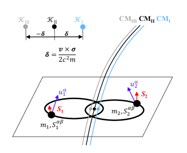
Figure 1: Different world lines of the center of spinning masses. Three centers of mass (CMs) have been demonstrated for each SSC.

III Generalized mechanics of spinning two-body systems

Consider a compact two-body system with leading-order spin-orbit interaction, where masses are $m_{i}$ and spins are $\mathbf{S}_{\mathbf{i}}$ ($i=1,2$). The equation of motion (relative acceleration) for the three different SSCs can be found in Ref. Kidder as

$$\mathbf{a} = -\frac{Gm}{r^{3}}\mathbf{r+}{\frac{G}{c^{2}r^{3}}}\Biggl{\{}{\frac{3}{r^{2}}}\mathbf{r}\left[(\mathbf{r}\times\mathbf{v})\cdot\left(2\mathbf{S}+(1+k)\mbox{\boldmath$\sigma$}\right)\right]$$ (7)

$$-\mathbf{v\times(}4\mathbf{S}+3{\mbox{\boldmath$\sigma$})}+{\frac{3\dot{r}}{r}}\mathbf{r}\times(2\mathbf{S}+(2-k){\mbox{\boldmath$\sigma$}})\Biggr{\}},$$

where $r=\left|\mathbf{r}\right|$ and $\mathbf{v}$ are the relative distance and velocity, respectively, $m=m_{1}+m_{2}$ is the total mass of the system where the masses $m_{1}$ and $m_{2}$, and the overdot denotes the derivative with respect to the time, $\mathbf{S}=\mathbf{S}_{1}+\mathbf{S}_{2}$ is the total spin vector and ${\mbox{\boldmath$\sigma$}}=(m_{2}/m_{1})\mathbf{S}_{1}+(m_{1}/m_{2})\mathbf{S}_{2}$ is the weighted spin vector where the individual spins $\mathbf{S}_{1}$ and $\mathbf{S}_{2}$ follow the notations of Ref. GPV3 . Here we have introduced the SSC-dependent parameter $k$ with the following values for the different SSCs

$$k=\left\{\begin{array}[]{ll}1&\text{for SSC I, }\\ {\frac{1}{2}}&\text{for SSC II, }\\ 0&\text{for SSC III. }\end{array}\right.$$ (8)

The transformation between the SSCs (see Fig. 1) is given by Ref. Kidder as

$$\mathbf{r}^{(k)} = \mathbf{r}^{(k\prime)}+\frac{k^{\prime}-k}{c^{2}m}\mathbf{v}\times{\mbox{\boldmath$\sigma$}}\ ,$$ (9)

$$\mathbf{v}^{(k)} = \mathbf{v}^{(k\prime)}+\frac{G(k-k^{\prime})}{c^{2}r^{3}}\mathbf{r}\times{\mbox{\boldmath$\sigma$}}\ .$$ (10)

Then we can compute the corresponding Lagrangian from the acceleration in Ref. KWW for SSC I and Ref. Kepler for SSC II, as

$$\mathcal{L} = \frac{\mu}{2}\mathbf{v}^{2}+\frac{Gm\mu}{r}+\frac{G\mu}{c^{2}r^{3}}\mathbf{v\cdot}\left[\mathbf{r}\times\left(2\mathbf{S}+(1+k){\mbox{\boldmath$\sigma$}}\right)\right]$$ (11)

$$+\frac{(2k-1)\mu}{2c^{2}m}\mathbf{v}\cdot(\mathbf{a}\times{\mbox{\boldmath$\sigma$})},$$

where $\mu=m_{1}m_{2}/m$ is the reduced mass. It can be seen that the only case in which the Lagrangian does not depend on acceleration terms is that of SSC II (for $k=1/2$). According to Ref. S84 the infinitesimal acceleration dependence can be eliminated by a time-coordinate transformation. Here only the $k=1/2$ case is relevant, but in this way the SSC dependence is shifted in the coordinates. Note that the acceleration dependence can be eliminated if we use the Newtonian-order acceleration $\mathbf{a}_{N}=-(Gm/r^{3})\mathbf{r}$ in Eq. (11) ; thus, we get the case of SSC II. The generalized moments can be calculated by the generalized Lagrangian as

$$\mathbf{p}=\frac{\partial\mathcal{L}}{\partial\mathbf{\dot{r}}}-\mathbf{\dot{q}},\qquad\mathbf{q}=\frac{\partial\mathcal{L}}{\partial\mathbf{a}},$$ (12)

yields to

$$\mathbf{p}=\mu\mathbf{\dot{r}}+\frac{G\mu}{c^{2}r^{3}}\mathbf{r}\times\left[2\mathbf{S}+(2-k){\mbox{\boldmath$\sigma$}}\right],\qquad\mathbf{q}=\frac{(2k-1)\mu}{2c^{2}m}{\mbox{\boldmath$\sigma$}}\times\mathbf{\dot{r}}.$$ (13)

The energy and the orbital angular momentum from acceleration-dependent Lagrangian dynamics are respectively

$$E = \mathbf{p}\cdot\mathbf{v+q}\cdot\mathbf{a-}\mathcal{L},$$ (14)

$$\mathbf{L} = \mathbf{r}\times\mathbf{p+v}\times\mathbf{q}.$$ (15)

The energy $E$, the magnitude of the orbital angular momentum $L=\left|\mathbf{L}\right|$, the magnitudes of the spinvectors $S_{i}$ and the total angular momentum vector $\mathbf{J}=\mathbf{L}+\mathbf{S}$ are conserved quantities. We compute the energy and the orbital angular momentum for different SSCs using Eqs. (14) and (15),

$$E = \frac{\mu}{2}\mathbf{v}^{2}-\frac{Gm\mu}{r}+\frac{G\mu(1-2k)}{c^{2}r^{3}}\mathbf{v}\cdot\left(\mathbf{r}\times{\mbox{\boldmath$\sigma$}}\right),$$ (16)

$$\mathbf{L} = \mu\mathbf{r}\times\mathbf{v}+\frac{G\mu}{c^{2}r^{3}}\mathbf{r}\times\left[\mathbf{r}\times\left(2\mathbf{S}+(2-k){\mbox{\boldmath$\sigma$}}\right)\right]$$ (17)

$$+\frac{(1-2k)\mu}{2c^{2}m}\mathbf{v}\times\left(\mathbf{v}\times{\mbox{\boldmath$\sigma$}}\right).$$

Here the main conserved quantities, i.e., the energy $E$ and the magnitude of orbital angular momentum $L$, depend on SSC although we do not mark the SSC dependence ($k$ dependence) on $E$ and $L$. If we set $k=1/2$ the Lagrangian does not depend on the acceleration.

Considering the canonical dynamics the first Hamiltonian description of the spin-orbit interaction for compact binary systems in SSC II was given by Refs. Wex ,Gopa , and Tessmer , we can calculate the Hamiltonian from (acceleration-dependent) Lagrangian for all SSCs. The generalized Hamiltonian from a generalized Legendre transformation is

$$\mathcal{H}=\mathbf{p}\cdot\mathbf{v}+\mathbf{q}\cdot\mathbf{a}-\mathcal{L}.$$ (18)

Here we should eliminate the acceleration terms from the Hamiltonian, Eq. (18); thus, we need to use the acceleration in Eq. (7). Two canonical pairs appear here, which are $(\mathbf{r},\mathbf{p})$ and $(\mathbf{v},\mathbf{q})$. This is nontrivial because we do not know which canonical moment to use in the Legendre transformation. After using the canonical moment $\mathbf{p}$ in Eq. (13), we can calculate the Hamiltonian

$$\mathcal{H} = \frac{\mathbf{p}^{2}}{2\mu}-\frac{Gm\mu}{r}$$ (19)

$$+\frac{G}{2c^{2}r^{3}}\mathbf{r}\cdot\biggl{[}2\mathbf{p}\times\left(2\mathbf{S}+(2-k){\mbox{\boldmath$\sigma$}}\right)$$

$$+(2k-1)\mu\mathbf{v}\times{\mbox{\boldmath$\sigma$}}\biggr{]}-\frac{Gm}{r^{3}}\mathbf{q}\cdot\mathbf{r}$$

$$\mathbf{-}{\frac{G}{c^{2}\mu r^{3}}}\mathbf{q}\cdot\Biggl{\{}\mathbf{p\times(}4\mathbf{S}+3{\mbox{\boldmath$\sigma$})}$$

$$-\mathbf{r}\left[(\mathbf{r}\times\mathbf{p})\cdot(2\mathbf{S}+(1+k)\mbox{\boldmath$\sigma$})\right]$$

$$-{\frac{3(\mathbf{r}\cdot\mathbf{p)}}{r^{2}}}\mathbf{r}\times(2\mathbf{S}+(2-k){\mbox{\boldmath$\sigma$}})\Biggr{\}}.$$

Note that we had to add an extra term $(1-2k)G/(2c^{2}r^{3})\left(\mu\mathbf{v-p}\right)\cdot(\mathbf{r}\times{\mbox{\boldmath$\sigma$})}$ (which disappears if we use the zeroth-order canonical moment $\mathbf{p}$) to the original Hamiltonian in Eq. (18); otherwise, it could not satisfy the generalized Hamilton’s equations

$$\mathbf{\dot{p}} = -\frac{\partial\mathcal{H}}{\partial\mathbf{r}},\qquad\mathbf{\dot{r}}\mathbf{=}\frac{\partial\mathcal{H}}{\partial\mathbf{p}},$$ (20)

$$\mathbf{\dot{q}} = -\frac{\partial\mathcal{H}}{\partial\mathbf{v}},\qquad\mathbf{\dot{v}=}\frac{\partial\mathcal{H}}{\partial\mathbf{q}}.$$ (21)

Then the explicit Hamilton’s equations up to $\mathcal{O}(c^{-2})$ are

$$\mathbf{\dot{p}} = -\frac{Gm\mu}{r^{3}}\mathbf{r}-\frac{G}{c^{2}r^{3}}\mathbf{p}\times\left[2\mathbf{S}+(1+k){\mbox{\boldmath$\sigma$}}\right]$$ (22)

$$+\frac{3G}{c^{2}r^{5}}\mathbf{r}\left[(\mathbf{r}\times\mathbf{p})\cdot(2\mathbf{S}+(1+k)\mbox{\boldmath$\sigma$})\right],$$

$$\mathbf{\dot{r}} \mathbf{=} \frac{\mathbf{p}}{\mu}-\frac{G}{c^{2}r^{3}}\mathbf{r}\times\left[2\mathbf{S}+(2-k){\mbox{\boldmath$\sigma$}}\right],$$ (23)

$$\mathbf{\dot{q}} \mathbf{=} \frac{G\mu(2k-1)}{2c^{2}r^{3}}\mathbf{r}\times\mbox{\boldmath$\sigma$}\mathbf{,}$$ (24)

$$\mathbf{\dot{v}} \mathbf{=} -\frac{Gm}{r^{3}}\mathbf{r-}{\frac{G}{c^{2}\mu r^{3}}}\Biggl{\{}\mathbf{p\times(}4\mathbf{S}+3{\mbox{\boldmath$\sigma$})}$$ (25)

$$-{\frac{3}{r^{2}}}\mathbf{r}\left[(\mathbf{r}\times\mathbf{p})\cdot(2\mathbf{S}+(1+k)\mbox{\boldmath$\sigma$})\right]$$

$$-\frac{3(\mathbf{r}\cdot\mathbf{p)}}{r^{2}}\mathbf{r}\times(2\mathbf{S}+(2-k){\mbox{\boldmath$\sigma$}})\Biggr{\}},$$

where in Eqs. (22) and (23) we used the approximation $\mathcal{O}(\mathbf{q})\mathcal{O}(c^{-2})\approx 0$, which can be seen from Eq. (13) or Eq. (24). Equation (24) disappears for SSC II and Eqs. (22) and (23) will be equivalent to Eq. (25) which is the acceleration Eq. (7) in the Lagrangian method. In Appendices A and B we show two different methods for the elimination of the acceleration-dependent terms from the Lagrangian.

III.1 Canonical structure

We define the generalized Poisson brackets following the paper of Ref. YH80 , where $f$ and $g$ functions arbitrarily depend on the canonical and spin variables

$$\left\{f,g\right\}=\sum_{j,i=1}^{3,2}\left[\frac{\partial f}{\partial\mathbf{Q}_{i}^{j}}\frac{\partial g}{\partial\mathbf{P}_{i}^{j}}-\frac{\partial f}{\partial\mathbf{P}_{i}^{j}}\frac{\partial g}{\partial\mathbf{Q}_{i}^{j}}-\frac{\partial f}{\partial\mathbf{S}_{i}^{j}}\left(\mathbf{S}_{i}^{j}\times\frac{\partial g}{\partial\mathbf{S}_{i}^{j}}\right)\right],$$ (26)

where $\mathbf{Q}_{1}\equiv\mathbf{r}$, $\mathbf{Q}_{2}\equiv\mathbf{v}$, $\mathbf{P}_{1}\equiv\mathbf{p}$ and $\mathbf{P}_{2}\equiv\mathbf{q}$ are useful vector notations, and the superscripts are the components of the vectors. Thus, the nonvanishing fundamental Poisson brackets are

$$\left\{P_{i}^{l},Q_{j}^{k}\right\} = \delta_{ij}\delta_{lk},$$ (27)

$$\left\{S_{i}^{l},S_{j}^{k}\right\} = \delta_{ij}\varepsilon_{lkm}S_{i}^{m}.$$ (28)

The time evolutions are given by their Poisson brackets with the Hamiltonian, so the generalized Hamilton’s equations can be written as

$$\mathbf{\dot{P}}_{i} \mathbf{=} \left\{\mathbf{P}_{i}\mathbf{,}\mathcal{H}\right\},$$ (29)

$$\mathbf{\dot{Q}}_{i} \mathbf{=} \left\{\mathbf{Q}_{i}\mathbf{,}\mathcal{H}\right\}.$$ (30)

The time evolution of the spins, the orbital angular momentum, and the Laplace-Runge-Lenz vector can be computed using of the fundamental Poisson brackets Eqs. (27) and (28)

$$\mathbf{\dot{S}}_{i} = \left\{\mathbf{S}_{i}\mathbf{,}\mathcal{H}\right\}=\frac{G(4+3\nu_{i})}{2c^{2}r^{3}}\mathbf{L}\times\mathbf{S}_{i},$$ (31)

$$\mathbf{\dot{L}} = \left\{\mathbf{L,}\mathcal{H}\right\}=\frac{G}{2c^{2}r^{3}}\left(4\mathbf{S}+3{\mbox{\boldmath$\sigma$}}\right)\times\mathbf{L,}$$ (32)

$$\mathbf{\dot{A}} = \left\{\mathbf{A,}\mathcal{H}\right\}=\frac{G}{c^{2}r^{3}}\left[2\mathbf{S}+(2-k){\mbox{\boldmath$\sigma$}}\right]\times\mathbf{A}$$ (33)

$$+\frac{3G}{c^{2}\mu r^{5}}\left(\mathbf{r}\times\mathbf{L}\right)\left[2\mathbf{L}\cdot\mathbf{S}+(1+k)\mathbf{L}\cdot{\mbox{\boldmath$\sigma$}}\right]$$

$$+\frac{G(2k-1)}{c^{2}r^{3}}\left[\frac{\mu v^{2}}{2}{\mbox{\boldmath$\sigma$}}\times\mathbf{r}+\mathbf{(L\cdot}\mbox{\boldmath$\sigma$}\mathbf{)v}\right].$$

with $\nu_{1}=\nu$ and $\nu_{2}=\nu^{-1}$ as shorthand notations where $\nu=$ $m_{2}/m_{1}$ is the mass ratio of the compact binary and $\mathbf{A=}\frac{\mathbf{p}}{\mu}\times\mathbf{L-}\frac{Gm\mu}{r}\mathbf{r}$ is the Laplace-Runge-Lenz (LRL) vector. To derive explicit evolution equations, we had to use the integration of the equation $\mathbf{\dot{q}}\mathbf{=}(2k-1)\mu/(2c^{2}m){\mbox{\boldmath$\sigma$}}\times\mathbf{\dot{v}}$ from Eqs. (24) and (25). It can be seen that the time evolution of the LRL vector depends on SSC and is not a pure precession as in the case of $\mathbf{\dot{S}}_{i}$ and $\mathbf{\dot{L}}$.

IV The equations of motion

We need to compute the evolution of the angular momenta. The evolution of the Newtonian orbital angular momentum vector $\mathbf{L}_{\mathbf{N}}=\mu\mathbf{r}\times\mathbf{v}$ the first term in Eq. (17) does not follow a pure precession motion, since

$$\mathbf{\dot{L}}_{\mathbf{N}} = -\frac{\mu G}{c^{2}r^{3}}\mathbf{r}\times\left[\mathbf{v\times(}4\mathbf{S}+3{\mbox{\boldmath$\sigma$})}\right]$$ (34)

$$+\frac{3\mu G\dot{r}}{c^{2}r^{4}}\mathbf{r}\times\left[\mathbf{r}\times(2\mathbf{S}+(2-k){\mbox{\boldmath$\sigma$}})\right];$$

meanwhile, the motion of the total orbital angular momentum vector $\mathbf{L}$ leads to a pure precession equation from Eq. (32),

$$\mathbf{\dot{L}}\mathbf{=}\frac{G}{2c^{2}r^{3}}\left(4\mathbf{S}+3{\mbox{\boldmath$\sigma$}}\right)\times\mathbf{L}.$$ (35)

This pure precession can be given by the conservation of the total angular momentum ($\mathbf{\dot{J}}=0$), and as a consequence $\mathbf{\dot{L}=-\dot{S}}$. This way the motion of the total spin vector does not have pure precession, but the individual spin vectors of the orbiting bodies do have one in Eq. (31) or in Ref. BOC74 . It can be seen that the pure precession equation for the total angular momentum vector does not depend on SSC, but the evolution of the Newtonian angular momentum vector depends on SSC; see Eqs. (35) and (34), respectively, and Fig 2. We may get different angular equations depending on which orbital momentum vectors ($\mathbf{L}_{\mathbf{N}}$ or $\mathbf{L}$) we measure with the Euler angles. The radial motion is invariant to this choice. Hereafter, we only consider the orbital motion involved in dynamical quantities fixed to $\mathbf{L}_{\mathbf{N}}$, where we will give the full radial motion for each of the other SSCs and we neglect the total angular motion (see Refs. Wex ; GPV3 ; Gopa ; Racine ; Tessmer ; recoil ).

We compute the orbital evolution using the conserved quantities $E$ and $L$ in Eqs. (16) and (17) for different SSCs. The first integrals can be separated into radial and angular motion. The radial and angular motion from energy and the magnitude of the orbital angular momentum are governed by

$$\dot{r}^{2} = \dot{r}_{N}^{2}-\frac{2G}{c^{2}\mu r^{3}}(2\mathbf{L}\cdot\mathbf{S}+(2-k)\mathbf{L}\cdot{\mbox{\boldmath$\sigma$})}$$ (36)

$$+\frac{2(2k-1)E}{c^{2}m\mu^{2}r^{2}}(\mathbf{L}\cdot{\mbox{\boldmath$\sigma$}),}$$

$$\dot{\varphi} = \dot{\varphi}_{N}+\frac{G}{c^{2}Lr^{3}}(2\mathbf{L}\cdot\mathbf{S}+3(1-k)\mathbf{L}\cdot{\mbox{\boldmath$\sigma$})}$$ (37)

$${-}\frac{(2k-1)E}{c^{2}m\mu Lr^{2}}(\mathbf{L}\cdot{\mbox{\boldmath$\sigma$}),}$$

where $\varphi$ is the azimuthal angle on the orbital plane. We have introduced the Newtonian formulas where $\dot{r}_{N}^{2}=2E\mu^{-1}+2Gmr^{-1}-L^{2}r^{-2}\mu^{-2}$ and $\dot{\varphi}_{N}=L\mu^{-1}r^{-2}$. We neglected the precession of the orbital plane. Accordingly, we have assumed that $(\mathbf{\hat{r}\times\hat{v})\propto\hat{L}}$ for derivation of the angular equation in Eq. (37). It means that the inclination angle between the total angular momentum $\mathbf{J}$ and the orbital angular momentum $\mathbf{L}$ is constant because the evolution of the angle is squared in magnitude of spin $d/dt(\mathbf{\hat{L}}\cdot\mathbf{\hat{J}})\approx\mathcal{O}(S^{2})$ (for SSC II see Ref. recoil ). In other words, it means that the orbital angular momentum $\mathbf{L}$ from Eq. (17) determines the orbital plane instead of the Newtonian angular momentum $\mathbf{L}_{\mathbf{N}}=\mu(\mathbf{r\times v)}$ (for SSC II see Ref. Gopa ). If we consider the unit angular momentum vector $\mathbf{\hat{L}}=(\mathbf{\hat{r}\times\hat{v})(}1+\delta)$ from Eq. (17), where $\delta$ is the leading-order perturbation, then the angular equation is $\dot{\varphi}=$ $L\mu^{-1}r^{-2}(1-\delta)$; see Eq. (37). We have assumed that the scalar products $\mathbf{L}\cdot\mathbf{S}$ and $\mathbf{L}\cdot{\mbox{\boldmath$\sigma$}}$ are constant because they appear in the perturbative terms of $\mathcal{O}(c^{-2})$ or the evolution of scalar products $\mathbf{S_{i}\cdot L}_{\mathbf{N}}$ (or $\mathbf{S_{i}\cdot L}$) represents first-order effects, see Ref. GPV3 . The radial equation agrees with the expressions of Refs. Wex and GPV3 for SSC I ($k=1$) and SSC II ($k=2$), respectively. $\mathbf{L}$ and $\mathbf{L}_{\mathbf{N}}$ appearing in perturbations are freely interchangeable in scalar products because we have eliminated the quadratic terms in spin $\mathcal{O}(S^{2})$.

Generally there are three angular equations with Euler angles (i.e., $\varphi,\Upsilon,\Theta_{N}$) for spin-orbit interaction given by Ref. recoil as

$$\dot{\varphi} = \frac{L}{{\mu}r^{2}}\left(1-\frac{\lambda_{SO}}{2{L}^{2}}\right)-\cos\Theta_{N}\ \dot{\Upsilon},$$ (38)

$$\dot{\Upsilon} = \frac{\tan\varphi}{\sin\Theta_{N}}\dot{\Theta}_{N},$$ (39)

where $\lambda_{SO}$ is a shorthand notation for the SO contributions in Eq. (38) that we have computed for all SSCs. $\lambda_{SO}=-2G\mu L/(c^{2}r)\left[2\mathcal{S}\mathbf{+}3\left(1-k\right)\Sigma\right]+2(2k-1)EL/(c^{2}m)\Sigma$, which corresponds to the two SO correction terms in Eq. (37). Here we used the original notations of Ref. Wex , where $\varphi=\psi$, $\Upsilon=-\phi_{n}$, $\Theta_{N}=\mathbf{\hat{J}}\cdot\mathbf{\hat{L}}_{\mathbf{N}}$ and $\Theta=\mathbf{\hat{J}}\cdot\mathbf{\hat{L}}$ in the Hamiltonian formalism. It can be seen that if we do not take the evolution of the angle $\Theta$ into account, we get Eq. (37) from Eqs. (38) and (39). In addition,

$$\dot{\Theta}_{N} = -\frac{G\mu\left(\mathbf{S\cdot v}\right)}{c^{2}JL_{N}r^{3}}\mathbf{[}4(\mathbf{S\cdot r)}+3({\mbox{\boldmath$\sigma$}\mathbf{\cdot r)}]}$$ (40)

$${+\frac{3G\mu\dot{r}\left({\mathbf{S\cdot r}}\right)}{c^{2}r^{4}}}\left[{2(\mathbf{S\cdot r)}+(2-k)({\mbox{\boldmath$\sigma$}}\mathbf{\cdot r)}}\right]$$

$$+\frac{G\mu\dot{r}\left(\mathbf{S}\cdot\mathbf{L}_{N}\right)}{c^{2}JL_{N}^{2}r^{2}}[2(\mathbf{S\cdot L}_{\mathbf{N}})+3(1-k)({\mbox{\boldmath$\sigma$}}\mathbf{\cdot L}_{\mathbf{N}})].$$

It is important to know that the polar angle $\Theta$ does not depend on SSC, but $\Theta_{N}$ does.

$$\dot{\Theta}=\frac{3G\mu\left(\nu^{-1}-\nu\right)}{2c^{2}Jr^{3}}\mathbf{L}\cdot\left(\mathbf{S}_{1}\times\mathbf{S}_{2}\right).$$ (41)

It can be seen that $\dot{\Theta}=0$ is relevant for two different cases: (i) equal mass ($\nu=1$) and (ii) single spin ($\mathbf{S}_{1}=0$ or $\mathbf{S}_{2}=0$) cases. The evolutions of the angles of $\Theta$ and $\Theta_{N}$ are quadratic in spin $\dot{\Theta},\dot{\Theta}_{N}\approx\mathcal{O}(S^{2})$.

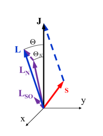
Figure 2: Total and Newtonian angular momenta. The angles of $\Theta$ and $\Theta_{N}$ are different but the evolution equations for the other two Euler angles are equivalent with each other.

V Orbital motion

Let us consider the radial motion which is characterized by Eq. (36). We will use the generalized true anomaly $\chi$ parametrization GPV3 ,Kepler

$$r=\frac{a_{r}(1-e_{r}^{2})}{1+e_{r}\cos\chi},$$ (42)

where $a_{r}$ is the semimajor axis and $e_{r}$ is the radial eccentricity. These parameters can be given by the turning points $\dot{r}^{2}=0$. Thus we have found that the solution is in the form $r_{{}_{{}_{min}^{max}}}=r_{\pm}(1+r_{\varepsilon})$, where $r_{\pm}=-(Gm\mu\pm A)/(2E)=L^{2}/[\mu(Gm\mu\mp A)]$ is the zeroth-order (or Newtonian) solution with $A^{2}=G^{2}m^{2}\mu^{2}+2EL^{2}/\mu$ and $r_{\varepsilon}$ is the linear-order perturbation. Here $A$ is a conserved quantity although it is not identical with the length of the LRL vector which is only conserved for the Newtonian order. Then, we get the turning points as

$$r_{{}_{{}_{min}^{max}}} = \frac{L^{2}}{\mu(Gm\mu\mp A)}+(A\mp Gm\mu)$$ (43)

$$\times\frac{4Gm\mu\mathcal{S}+\left[3Gm\mu\mp(1-2k)A\right]\Sigma}{2c^{2}mLA}.$$

Here we used the notations for conserved scalar products $\mathcal{S}=\mathbf{\hat{L}}\cdot\mathbf{S}$ and $\Sigma=\mathbf{\hat{L}}\cdot{\mbox{\boldmath$\sigma$}}$ (the evolution of these quantities are first-post Newtonian order effects, so we could use them in linear-order terms; see Ref. GPV3 ). The relationship between the orbital elements and turning points is $a_{r}=(r_{\max}+r_{\min})/2$ and $e_{r}=(r_{\max}-r_{\min})/(r_{\max}+r_{\min})$, so the radial orbital parameters in all SSCs are

$$a_{r} = \frac{Gm\mu}{-2E}+\frac{G\mu}{c^{2}L}\left[2\mathcal{S}+(2-k)\Sigma\right],$$ (44)

$$e_{r}^{2} = 1+\frac{2EL^{2}}{G^{2}m^{2}\mu^{3}}+\frac{4E}{c^{2}mL}\Biggl{\{}4\left[1+\frac{EL^{2}}{G^{2}m^{2}\mu^{3}}\right]\mathcal{S}$$ (45)

$$+\left[2\left(2-k\right)+\frac{\left(5-4k\right)EL^{2}}{G^{2}m^{2}\mu^{3}}\right]\Sigma\Biggr{\}}.$$

Then, the conserved quantities with orbital elements are

$$E = \frac{Gm\mu}{-2a_{r}}\Biggl{\{}1+\frac{G^{1/2}}{c^{2}m^{1/2}a_{r}^{3/2}(1-e_{r}^{2})^{1/2}}$$ (46)

$$\times\left(2\mathcal{S}+(2-k)\Sigma\right)\Biggr{\}},$$

$$L^{2} = Gm\mu^{2}a_{r}(1-e_{r}^{2})\Biggl{\{}1-\frac{G^{1/2}}{c^{2}m^{1/2}a_{r}^{3/2}(1-e_{r}^{2})^{3/2}}$$ (47)

$$\times\left[2(3+e_{r}^{2})\mathcal{S}+(5-k+3(1-k)e_{r}^{2})\Sigma\right]\Biggr{\}}.$$

The time evolution of the generalized true anomaly from Eq. (36) in terms of the orbital elements is

$$\frac{dt}{d\chi} = \frac{r^{2}}{\sqrt{Gma_{r}(1-e_{r}^{2})}}\Biggl{\{}1+\left(2\mathcal{S}+(2-k)\Sigma\right)$$ (48)

$$\times\frac{G^{1/2}\left(e_{r}^{2}-3-2e_{r}\cos\chi\right)}{2c^{2}m^{1/2}a_{r}^{3/2}(1-e_{r}^{2})^{3/2}}\Biggr{\}}.$$

After the integration we can get the result with eccentric anomaly $u$ parametrization, namely $r=a_{r}(1-e_{r}\cos u)$. In other papers (e.g., Kepler ) it is indicated as $\xi$ . Then we get the generalized Kepler equation which contains the spin-orbit contributions in all SSCs as

$$n(t-t_{0})=u-e_{t}\sin u,$$ (49)

where we have introduced two orbital elements which are the mean motion $n$ and the time eccentricity $e_{t}$ with conserved quantities ($E$, $L$, $\mathcal{S}$, and $\Sigma$),

$$n = \frac{1}{Gm}\left(\frac{-2E}{\mu}\right)^{3/2},$$ (50)

$$e_{t}^{2} = 1+\frac{2EL^{2}}{G^{2}m^{2}\mu^{3}}+\frac{4E}{c^{2}mL}$$ (51)

$$\times\Biggl{\{}2\mathcal{S}+\left[2-k+\frac{\left(1-2k\right)EL^{2}}{G^{2}m^{2}\mu^{3}}\right]\Sigma\Biggr{\}}.$$

It can be seen that the mean motion does not contain SO terms and the time eccentricity depends on SSC.

In the following let us consider the simple angular motion of the binary systems which is described by Eq. (37). As we have mentioned above, we solve the equation of motion in a noninertial frame, which is the orbital plane. Thus, the angular equation from Eq. (37) is

$$\dot{\varphi}=\frac{L}{\mu r^{2}}+\frac{\alpha}{r^{2}}+\frac{\beta}{r^{3}},$$ (52)

where we have introduced the shorthand notations

$$\alpha = {-}\frac{(2k-1)E\Sigma}{c^{2}m\mu},$$ (53)

$$\beta = \frac{G\left[2\mathcal{S}+3(1-k)\Sigma\right]}{c^{2}}.$$ (54)

Using the generalized true anomaly parametrization in Eq. (42) the angular equation Eq. (52) can be integrated in terms of the orbital elements

$$\frac{d\varphi}{d\chi}=1-\frac{G^{1/2}\left[4\mathcal{S}+3\Sigma-\left(1-2k\right)\Sigma e_{r}\cos\chi\right]}{c^{2}m^{1/2}a_{r}^{3/2}(1-e_{r}^{2})^{3/2}}\ .$$ (55)

After the integration we get the angular motion as (see Ref. MFV for the first post-Newtonian corrections)

$$\varphi-\varphi_{0}=K\chi-Q\sin\chi,$$ (56)

where $\varphi_{0}$ is the integration constant. We have also introduced some shorthand notations with conserved quantities

$$K = 1-\frac{G^{2}m\mu^{3}\left(4\mathcal{S}+3\Sigma\right)}{c^{2}L^{3}},$$ (57)

$$Q = \frac{G\mu^{2}\left(2k-1\right)A\Sigma}{c^{2}L^{3}}.$$ (58)

There is another solution for the angular evolution in literature, which is introduced by Damour and Deruelle in Ref. DD85 using the conchoidal transformation. In this parametrization there is a third eccentricity $e_{\theta}$. If we use the conchoidal transformation $r=\tilde{r}$ $+\beta/(2\tilde{L})$ with $\tilde{L}=L/\mu+\alpha$ in Eq.(52), then the angular equation has the simple form (like the Newtonian equation for the angular motion)

$$\dot{\varphi}=\frac{\tilde{L}}{\tilde{r}^{2}}.$$ (59)

The integration of this angular equation with the generalized eccentric anomaly parametrization $r=a_{r}(1-e_{r}\cos u)$, where we used the deformed parametrization

$$\tilde{r}=\tilde{a}\left(1-\tilde{e}\cos u\right),$$ (60)

with $\tilde{a}=a_{r}-\beta/(2\tilde{L})$ and $\tilde{e}=a_{r}e_{r}/\tilde{a}$ as shorthand notations is straightforward. With the help of Eqs. (60) and (49) in Eq. (59) we get

$$\frac{d\varphi}{du}=\frac{\tilde{L}}{n\tilde{a}^{2}(1-e_{\theta}\cos u)},$$ (61)

where we have introduced the angular eccentricity $e_{\theta}=2\tilde{e}-e_{t}$ as an orbital parameter. After the integration we get

$$\varphi-\varphi_{0}=(1+\tilde{k})v,$$ (62)

where $\tilde{k}=\tilde{L}/(n\tilde{a}^{2}\sqrt{1-e_{\theta}^{2}})-1$ is the pericenter drift and $v=2\arctan\left(\sqrt{(1+e_{\theta})/(1-e_{\theta})}\tan u/2\right)$ is a similar Damour-Deruelle true anomaly. Finally, we add the angular orbital elements with conserved quantities, as

$$\tilde{k} = {-}\frac{G^{2}m\mu^{3}\left(4\mathcal{S}+3\Sigma\right)}{c^{2}L^{3}},$$ (63)

$$e_{\theta}^{2} = 1+\frac{2EL^{2}}{G^{2}m^{2}\mu^{3}}$$ (64)

$$+\left(1+\frac{EL^{2}}{G^{2}m^{2}\mu^{3}}\right)\frac{4E(4\mathcal{S}+3\Sigma{)}}{c^{2}mL}.$$

The Damour-Deruelle angular orbital parameters $e_{\theta}$ and $\tilde{k}$ in Eqs. (63) and (64) are not SSC-dependent. This angular motion does not agree with cases of SSC I/II in Refs. Wex , CK , and KJ because in these cases they only considered the Newtonian term the first term in Eq. (37), but we have the same angular motion in Ref. Gopa , which is identical with the paper of Ref. Tessmer for the eccentric case (see the Appendix C).

Both parametrizations are equivalent to each other. Apparently Eq. (56) depends on SSC, but if we use the eccentric anomaly parametrization $u$, the SSC dependence disappears. The relationships between quantities for the angular motion are

$$K = 1+\tilde{k}$$ (65)

$$Q = \frac{Gm\mu^{2}A\rho}{2EL^{2}},$$ (66)

where we have introduced $\rho=1-e_{r}/e_{\theta}$ as a shorthand notation.

VI Dissipation under gravitational radiation

The energy and the orbital angular momentum change due to the gravitational radiation at 2.5 PN order. The instantaneous losses for the spin-orbit interaction were given by Kidder Kidder using SSC I. Some authors calculated the averaged losses for SSC I/II RS ; GPV3 ; CK . We compute these averaged losses for all SSCs including the missing SSC III. The multipolar momenta are necessary for computation of the energy and the angular momentum losses up to the SO order. The mass $\mathcal{I}_{ij}$ and current $\mathcal{J}_{ij}$ quadrupole momentums in relative Descartes coordinates are

$$\mathcal{I}_{ij} = \mu\left(r_{i}r_{j}\right)^{STF}$$ (67)

$$+\frac{2\eta}{3c^{2}}\left(\varepsilon_{ipq}\left[(1+3k)r_{j}v_{p}-2v_{j}r_{p}\right]{{\mbox{$\sigma$}}}_{q}\right)^{STF},$$

$$\mathcal{J}_{ij} = -\eta\delta m\left(\varepsilon_{ipq}r_{j}r_{p}v_{q}\right)^{STF}$$ (68)

$$+\frac{3\mu}{2\delta m}\left(r_{i}\left[S_{j}-{{\mbox{$\sigma$}}}_{j}\right]\right)^{STF},$$

where $\eta=\mu/m$ is the symmetric mass ratio, $x_{i}$ are relative coordinates, $v_{i}=\dot{x}_{i}$ is the relative velocity of the binary, $S_{i}$ and ${{\mbox{$\sigma$}}}_{i}$ are the coordinates of the spin vector $\mathbf{S}$ and $\sigma$, respectively, the mass difference $\delta m=m_{1}-m_{2}$ (choosing $m_{1}\geqq m_{2}$ by convention) and $\varepsilon_{ijk}$ is the Levi-Civita symbol. The last term is apparently singular for equal masses in Eq. (68) because it can be expressed as $(3/2)Gm(r_{i}\eta_{j})^{STF}$ with another spin vector ${\mbox{\boldmath$\eta$}}=\mu(\mathbf{S}_{1}/m_{1}-\mathbf{S}_{2}/m_{2})/(Gm^{2})$ (see Table I). It can be proved that the current angular momentum $\mathcal{J}_{ij}$ does not depend on SSC. Here $STF$ means the indices of the momentums $\mathcal{I}_{ij}$ and $\mathcal{J}_{ij}$ are symmetric-trace-free. Thus, the instantaneous energy and the angular momentum losses up to the SO order are given by KWW

$$\frac{dE}{dt} = -\frac{G}{5c^{5}}\left(\mathcal{\dddot{I}}_{ij}\mathcal{\dddot{I}}_{ij}+\frac{16}{9c^{2}}\mathcal{\dddot{J}}_{ij}\mathcal{\dddot{J}}_{ij}\right),$$ (69)

$$\frac{dL}{dt} = -\frac{2G}{5c^{5}}\varepsilon_{ipq}\left(\mathcal{\ddot{J}}_{pj}\mathcal{\dddot{I}}_{qj}+\frac{16}{9c^{2}}\mathcal{\ddot{J}}_{pj}\mathcal{\dddot{J}}_{qj}\right)\hat{L}_{i},$$ (70)

where repeated indices indicate summation, dots over multipolar moments mean time derivatives, and $\hat{L}_{i}$ denotes the components of the unit angular momentum vector in Eq. (17). Then we get the instantaneous losses for different SSCs

$$\frac{dE}{dt} = \frac{8G^{3}m^{2}\mu^{2}}{15c^{5}r^{4}}\left(11\dot{r}^{2}-12v^{2}\right)$$ (71)

$$-\frac{8G^{3}m\mu L}{15c^{7}r^{6}}\Biggl{\{}\left[27\dot{r}^{2}-37v^{2}-12\frac{Gm}{r}\right]\mathcal{S}$$

$$+\biggl{[}3(22k-5)\dot{r}^{2}-(48k-5)v^{2}$$

$$+4(6k-5)\frac{Gm}{r}\biggr{]}\Sigma\Biggr{\}},$$

$$\frac{dL}{dt} = \frac{8G^{2}m\mu L}{5c^{5}r^{5}}\left(3\dot{r}^{2}-2v^{2}-\frac{2Gm}{r}\right)$$ (72)

$$+\frac{12G^{2}\mu^{2}}{45c^{7}r^{7}}\Biggl{\{}\biggl{[}6\left(3\dot{r}^{2}v^{2}-4\dot{r}^{4}+v^{4}\right)$$

$$-26\frac{Gm}{r}\left(\dot{r}^{2}-v^{2}\right)-6\frac{G^{2}m^{2}}{r^{2}}\biggr{]}\mathcal{S}$$

$$+\biggl{[}6(16-21k)\dot{r}^{2}v^{2}-(78-90k)\dot{r}^{4}$$

$$-(17-36k)v^{4}+\frac{Gm}{r}[(7-24k)\dot{r}^{2}$$

$$-8(1-3k)v^{2}]-5\frac{G^{2}m^{2}}{r^{2}}\biggr{]}\Sigma\Biggr{\}},$$

where $\mathcal{S=}\mathbf{\hat{L}}\cdot\mathbf{S}$ and $\Sigma\mathcal{=}\mathbf{\hat{L}}\cdot{\mbox{\boldmath$\sigma$}}$. It can be seen that our results are equivalent with that of Ref. Kidder for $k=1$ and Ref. RS for $k=1/2$.

The instantaneous energy and the angular momentum losses depend on SSC in Eqs. (71) and (72), so these formulas involve parameter $k$. If we use the $E$ and $L$ conserved quantities instead of $r$, $v$ and $\dot{r}$, the dependence on parameter $k$ remains. On the other hand, if we average these formulas for one Newtonian orbital period (see Ref. BOC70 ), the explicit $k$ dependence disappears, but $E$ and $L$ depend on SSC as in Eqs. (16) and (17)(see Fig. 3).

$$\left\langle{\frac{dE}{dt}}\right\rangle = -\frac{G^{2}m(-2E\mu)^{3/2}}{15c^{5}L^{7}}(148E^{2}L^{4}+732G^{2}m^{2}\mu^{3}EL$$ (73)

$$+425G^{4}m^{4}\mu^{6})+\frac{G^{2}(-2E\mu)^{3/2}}{10c^{7}L^{9}}\biggl{[}(520E^{3}L^{6}$$

$$+10740G^{2}m^{2}\mu^{3}E^{2}L^{4}+24990G^{4}m^{4}\mu^{6}EL^{2}$$

$$+12579G^{6}m^{6}\mu^{9})\mathcal{S}+(256E^{3}L^{6}$$

$$+6660G^{2}m^{2}\mu^{3}E^{2}L^{4}+16660G^{4}m^{4}\mu^{6}EL^{2}$$

$$+8673G^{6}m^{6}\mu^{9})\Sigma\biggr{]},$$

$$\left\langle{\frac{dL}{dt}}\right\rangle = -\frac{4G^{2}m(-2E\mu)^{3/2}}{5c^{5}L^{4}}(14EL^{2}+15G^{2}m^{2}\mu^{3})$$ (74)

$$+\frac{G^{2}(-2E\mu)^{3/2}}{15c^{7}L^{6}}\biggl{[}(1188E^{2}L^{4}$$

$$+6756G^{2}m^{2}\mu^{3}EL^{2}+5345G^{4}m^{4}\mu^{6})\mathcal{S}$$

$$+(772E^{2}L^{4}+4476G^{2}m^{2}\mu^{3}EL^{2}$$

$$+3665G^{4}m^{4}\mu^{6})\Sigma\biggr{]}.$$

We will compute the SO contributions of the waveform for different SSCs in the next chapter.

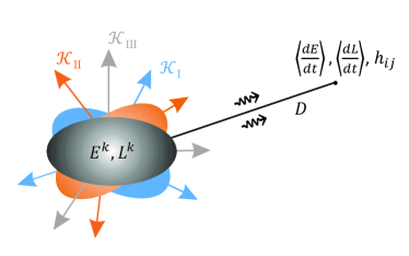
Figure 3: Dissipative quantities in the different SSCs. The compact binary system is characterized by the energy $E$ and the magnitude of the orbital angular momentum $L$, which depend on SSC (here $k$ means the SSC dependence). Here $D$ is the luminosity distance and $\mathcal{K}_{I,II,III}$ are the different frames for SSCs. Thus, the averaged energy and the orbital angular momentum losses due to gravitational radiation depend on SSC, however the leading-order spin-orbit waveform does not depend on SSC.

VII Waveform

We need the current octopole momentum $\mathcal{J}_{ijk}$ for the computation of the waveform $h_{ij}$ (see Eq. (3.20b) in Ref. Kidder ). Thus, the $\mathcal{J}_{ijk}$ does not depend on SSC up to the SO-order as

$$\mathcal{J}_{ijk} = \mu(1-3\eta)\left(r_{i}r_{j}\varepsilon_{kpq}r_{p}v_{q}\right)^{STF}$$ (75)

$$+2\eta\left(r_{i}r_{j}{{\mbox{$\sigma$}}}_{k}\right)^{STF}.$$

The second term in Eq. (75) is relevant for the computation of the waveform, as the first term only appears in the next PN-order corrections. The waveform up to the SO order is computed by

$$h_{ij} = \frac{2G}{c^{4}D}\biggl{[}\mathcal{\ddot{I}}_{ij}+\frac{4}{3c^{2}}\varepsilon_{kl(i}\mathcal{\ddot{J}}_{j)k}N_{l}$$ (76)

$$+\frac{1}{2c^{2}}\varepsilon_{kl(i}\mathcal{\dddot{J}}_{j)km}N_{l}N_{m}\biggr{]}_{TT},$$

where $D$ is the distance between the source and observer, $N_{k}$ are the components of the unit vector $\mathbf{N}$ which points from the source to the observer, and $(..)_{TT}$ means the transverse-traceless transformation (we have omitted the pure relativistic PN corrections, so the first terms in Eqs. (75,68) can be neglected).

The gravitational waveforms for all SSCs (here we have neglected the pure relativistic corrections $P^{0.5-1.5}Q_{ij}$ which are given in WW ,Wiseman ) are given as

$$h_{ij}=\frac{2G\mu}{c^{4}D}\left[Q_{ij}+PQ_{ij}^{SO}+P^{1.5}Q_{ij}^{SO}\right]_{TT},$$ (77)

with

$$Q_{ij} = 2\left(v_{i}v_{j}-\frac{Gm}{r^{3}}r_{i}r_{j}\right),$$ (78)

$$PQ_{ij}^{SO} = \frac{2m}{r^{3}\delta m}\Bigl{\{}\left[\left({\mbox{\boldmath$\sigma$}-\mathbf{S}}\right){\times}\mathbf{N}\right]_{(i}r_{j)}\Bigr{\}},$$ (79)

$$P^{1.5}Q_{ij}^{SO} = \frac{2}{r^{3}}\Biggl{\{}\frac{3r_{i}r_{j}}{r^{2}}(\mathbf{r\times v})\mathbf{\cdot}\left[2\mathbf{S}+(1+k)\mbox{\boldmath$\sigma$}\right]$$ (80)

$$-r_{(i}[\mathbf{v\times(}4\mathbf{S}+(3+2k)\mbox{\boldmath$\sigma$})]_{j)}$$

$$-2kv_{(i}(\mathbf{r\times}\mbox{\boldmath$\sigma$})_{j)}+\frac{6\dot{r}}{r}r_{(i}[\mathbf{r\times(S}+\mbox{\boldmath$\sigma$})]_{j)}$$

$$+\biggl{[}\left(\frac{3\dot{r}}{r}\mathbf{r}-2\mathbf{v}\right)(\mathbf{N\cdot r})$$

$$-2\mathbf{r}(\mathbf{N\cdot v})\biggr{]}_{(i}(\mbox{\boldmath$\sigma$}\mathbf{\times N)}_{j)}\Biggr{\}},$$

where we have used the following formulas which are valid for any TT-tensor and $\mathbf{a}$ and $\mathbf{b}$ vectors

$$\left(\delta_{ij}\right)_{TT} = \left(N_{i}b_{j}\right)_{TT}=0,$$

$$\left[b_{i}\left(\mathbf{a\times N}\right)_{j}\right]_{TT} = \left[a_{i}\left(\mathbf{b\times N}\right)_{j}\right]_{TT},$$ (81)

where $\delta_{ij}$ is the Kronecker delta function. The tensor $Q_{ij}$ is the zeroth-order waveform, the $PQ_{ij}^{SO}$ is the leading-order SO contribution (which does not contain terms $\mathcal{O}(\mathbf{N})$) and the $P^{1.5}Q_{ij}^{SO}$ is the next-to-leading-order SO contribution (which is proportional to terms $\mathcal{O}(\mathbf{N}^{0})$ and $\mathcal{O}(\mathbf{N}^{2})$ ) to the waveform. The leading-order SO contribution $PQ_{ij}^{SO}$ is singular for equal-masses, since $({\mbox{\boldmath$\sigma$}-\mathbf{S)/}}\delta m{\mathbf{\equiv S}}_{2}/m_{2}-{\mathbf{S}}_{1}/m_{1}$. Here we can use the spinvector $\mathbf{\Delta}$ of Kidder (see Table I). It is transparent that for $k=1$ we retain the SSC I case as in the classical paper of Kidder .

spinvectors	$(\mathbf{S}_{1},\mathbf{S}_{2})$	$({\mathbf{S,}\mbox{\boldmath$\sigma$})}$	$({\mathbf{S,}}\mathbf{\Delta)}$	$(\bm{\chi}_{s},\bm{\chi}_{a})$
$(\mathbf{S}_{1},\mathbf{S}_{2})$	-	$\begin{array}[]{c}{\mathbf{S=S}}_{1}+{\mathbf{S}}_{2},\\ {\mbox{\boldmath$\sigma$}}=\frac{m_{2}}{m_{1}}\mathbf{S}_{1}+\frac{m_{1}}{m_{2}}\mathbf{S}_{2}\end{array}$	$\begin{array}[]{c}{\mathbf{S=S}}_{1}+{\mathbf{S}}_{2}\text{, }\\ \mathbf{\Delta}=m\left(\frac{\mathbf{S}_{2}}{m_{2}}-\frac{\mathbf{S}_{1}}{m_{1}}\right)\end{array}$	$\begin{array}[]{c}\bm{\chi}_{s}=\frac{1}{2}\left(\frac{\mathbf{S}_{2}}{m_{2}^{2}}+\frac{\mathbf{S}_{1}}{m_{1}^{2}}\right)\text{, }\\ \bm{\chi}_{a}=\frac{1}{2}\left(\frac{\mathbf{S}_{2}}{m_{2}^{2}}-\frac{\mathbf{S}_{1}}{m_{1}^{2}}\right)\end{array}$
$({\mathbf{S,}\mbox{\boldmath$\sigma$})}$	$\begin{array}[]{c}{\mathbf{S}}_{1}{\mathbf{=}}\frac{\nu^{-1}{\mathbf{S}}-{\mbox{\boldmath$\sigma$}}}{\nu^{-1}-\nu},\\ {\mathbf{S}}_{2}=\frac{\nu{\mathbf{S}}-{\mbox{\boldmath$\sigma$}}}{\nu-\nu^{-1}}\end{array}$	-	$\mathbf{\Delta=}\frac{1+\nu}{1-\nu}\left({\mbox{\boldmath$\sigma$}-\mathbf{S}}\right)$	$\begin{array}[]{c}\bm{\chi}_{s}\mathbf{=}\frac{{{(1+\nu)}^{2}\mathbf{S+}(1-\nu^{2})\mathbf{\Delta}}}{2m^{2}{\nu}}\text{, }\\ \bm{\chi}_{a}\mathbf{=}\frac{\left(1+\nu\right)^{2}\left(\mathbf{S-\Delta}\right)}{2m^{2}{\nu}}\end{array}$
$({\mathbf{S,}}\mathbf{\Delta)}$	$\begin{array}[]{c}{\mathbf{S}}_{1}{\mathbf{=}}\frac{\left(\nu^{-1}-\nu\right){\mathbf{S}}\mathbf{-}\left(1-\nu\right)\mathbf{\Delta}}{\nu^{-1}+1-\nu-\nu^{2}},\\ {\mathbf{S}}_{2}=\frac{\left(1-\nu^{2}\right){\mathbf{S+}}\left(1-\nu\right)\mathbf{\Delta}}{\nu^{-1}+1-\nu-\nu^{2}}\end{array}$	${\mbox{\boldmath$\sigma$}}\mathbf{=S+}\frac{1-\nu}{1+\nu}\mathbf{\Delta}$	-	$\begin{array}[]{c}\bm{\chi}_{s}\mathbf{=}\frac{{(1+\nu)}^{2}{\mbox{\boldmath$\sigma$}}}{2m^{2}{\nu}}\text{, }\\ \bm{\chi}_{a}\mathbf{=}\frac{2\left(1+\nu\right){\mathbf{S-(}}1+\nu^{2})\left(1+\nu\right){\mbox{\boldmath$\sigma$}}}{2m^{2}{\nu}\left(1-\nu\right)}\end{array}$
$(\bm{\chi}_{s},\bm{\chi}_{a})$	$\begin{array}[]{c}\mathbf{S}_{1}=\frac{\nu m^{2}\left(\bm{\chi}_{s}-\bm{\chi}_{a}\right)}{(1+\nu)^{2}}\text{, }\\ \mathbf{S}_{2}=\frac{m^{2}\left(\bm{\chi}_{s}+\bm{\chi}_{a}\right)}{(1+\nu)^{2}}\end{array}$	$\begin{array}[]{c}{\mathbf{S}}\mathbf{=}\frac{m^{2}\left[\left(1-\nu^{2}\right)\bm{\chi}_{a}+{\mathbf{(}}1+\nu^{2})\bm{\chi}_{s}\right]}{(1+\nu)^{2}},\\ {\mbox{\boldmath$\sigma$}\mathbf{=}}\frac{2\nu m^{2}\bm{\chi}_{s}}{(1+\nu)^{2}}\end{array}$	$\begin{array}[]{c}{\mathbf{S=}}\frac{\nu m^{2}\left[\left(\nu^{-1}-\nu\right)\bm{\chi}_{a}+{\mathbf{(}}\nu^{-1}+\nu)\bm{\chi}_{s}\right]}{(1+\nu)^{2}}\text{, }\\ \mathbf{\Delta}=\frac{m^{2}\left[\left(1-\nu^{2}\right)\bm{\chi}_{a}+{\mathbf{(}}1+\nu^{2})\bm{\chi}_{s}\right]}{1-\nu^{2}}\end{array}$	-

Table 1: Different notations for spinvectors. One of the most widely used notations are the total ${\mathbf{S}}$ and the weighted $\sigma$ spins in GPV3 . ${\mathbf{S\equiv}\mbox{\boldmath$\zeta$}}$ and ${\mbox{\boldmath$\sigma$}\mathbf{\equiv}\mbox{\boldmath$\xi$}}$ in KWW Kidder , and RS (but here a factor $Gm^{2}$ is used in definitions, thus ${\mbox{\boldmath$\zeta$}}=({\mathbf{S}}_{1}+{\mathbf{S}}_{2})/Gm^{2}$ and ${\mbox{\boldmath$\xi$}}=\left(\nu\mathbf{S}_{1}+\nu^{-1}\mathbf{S}_{2}\right)/Gm^{2}$ where $\nu=m_{2}/m_{1}$ is the mass ratio parameter). The total and other combinations of weighted spins $\mathbf{\Delta=}(m/\delta m)\mathbf{(}\mbox{\boldmath$\sigma$}-\mathbf{S)}$ are also used in Kidder ,Blanchet , $\mathbf{\Sigma\equiv\Delta}$. Some authors used an effective spin combination $\mathbf{S}_{eff}=2{\mathbf{S+(}}3/2){\mbox{\boldmath$\sigma$}}$, which is a convenient notation for SSC II in Wex ; Gopa ; Tessmer ; Racine ; CK . There are other symmetrized spin quantities ${\mbox{\boldmath$\chi_{s}$}}=({\mathbf{S}}_{2}/m_{2}^{2}+{\mathbf{S}}_{1}/m_{1}^{2})/2$ and ${\mbox{\boldmath$\chi_{a}$}}=({\mathbf{S}}_{2}/m_{2}^{2}-{\mathbf{S}}_{1}/m_{1}^{2})/2$ which are useful notations for the dimensionless angular-momentum Kerr parameters of the individual bodies in Refs. WW ,Tagoshi .

VIII Summary

We presented the spin supplementary conditions for the leading-order spin-orbit contribution of compact binaries. The Lagrangian contains acceleration dependent terms in some cases of SSC. Thus we have to use the Ostrogradsky dynamics for generalized Lagrangian. We have shown some procedures of the elimination of the acceleration from the Lagrangian, i.e. the method of the double zero and constrained dynamics in Appendices. We constructed the generalized Hamiltonian function with the presence of high-order canonical moments and computed the generalized Hamilton’s equations.

Our radial and angular motion of the compact binaries represent the SSC dependence of any orbital parameters for eccentric orbits. We calculated the energy and the orbital angular momentum losses due to gravitational radiation in each SSC, and we concluded that the dependence of SSC apparently disappears, since we use averaging over one orbital period. However, these expressions are SSC-dependent because the energy and the orbital angular momentum depend on SSC, see Eqs. (14) and (15).

Nevertheless, we calculated the leading-order gravitational waveform contains the spin-orbit corrections. It has been proven that the leading-order spin-orbit does not depend on SSC but the next-to-leading-order spin-orbit contribution does.

IX Acknowledgements

I would like to thank Péter Forgács and Mátyás Vasúth for some critical reading of the manuscript. This work was supported by the Postdoctoral Fellowship Programme of the Hungarian Academy of Sciences and Hungarian Scientific Research Fund (OTKA) Grant No. 116892.

.1 Appendix A: The elimination of acceleration: Constrained dynamics

Constrained dynamics arose from the degenerate Lagrangian developed by Dirac, Anderson and Bergmann (see Dirac ; AB ). The simple acceleration-dependent Lagrangian of a relativistic spinning body studied by Riewe and Ellis leads to constrained dynamics. The Dirac formalism for constrained Hamiltonian of a spherical spinning top interacting with Poisson brackets was given by Ref. HRT .

We introduce two new variables using the method of Lagrange multipliers where ${\mbox{\boldmath$\lambda$}}\mathbf{=\dot{r}}$ for the acceleration term, and $\delta$ is a multiplier in the Lagrangian. The transformation of the Lagrangian is $\mathcal{L}(\mathbf{r},\mathbf{v,a})\rightarrow\mathcal{L}^{\ast}(\mathbf{r},\mathbf{v,{\mbox{\boldmath$\lambda$}},{\mbox{\boldmath${\dot{\lambda}}$}},}{\mbox{\boldmath$\delta$}})$ as

$$\mathcal{L}^{\ast} = \frac{\mu}{2}\mathbf{v}^{2}+\frac{Gm\mu}{r}+\frac{G\mu}{c^{2}r^{3}}\mathbf{v\cdot}\left[\mathbf{r}\times\left(2\mathbf{S}+(1+k){\mbox{\boldmath$\sigma$}}\right)\right]$$ (82)

$$+\frac{(2k-1)\mu}{2c^{2}m}\mathbf{v}\cdot({\mbox{\boldmath${\dot{\lambda}}$}}\times{\mbox{\boldmath$\sigma$})}+{\mbox{\boldmath$\delta$}}\mathbf{\cdot}(\mathbf{v}-{\mbox{\boldmath$\lambda$}}).$$

Then, the Euler-Lagrange equations are

$$\mu\mathbf{a} = -\frac{Gm\mu}{r^{3}}\mathbf{r}-\frac{2G\mu}{c^{2}r^{3}}\mathbf{v}\times\left(2\mathbf{S}+(1+k){\mbox{\boldmath$\sigma$}}\right)$$

$$+\frac{3G\mu}{c^{2}r^{5}}\mathbf{r}\left[\left(\mathbf{r}\times\mathbf{v}\right)\mathbf{\cdot}\left(2\mathbf{S}+(1+k){\mbox{\boldmath$\sigma$}}\right)\right]$$

$$\mathbf{+}\frac{3G\mu\dot{r}}{c^{2}r^{4}}\mathbf{r}\times\left(2\mathbf{S}+(1+k){\mbox{\boldmath$\sigma$}}\right)$$

$$-\frac{(2k-1)\mu}{2c^{2}m}({\mbox{\boldmath${\ddot{\lambda}}$}}\times{\mbox{\boldmath$\sigma$})-\mbox{\boldmath${\dot{\delta}}$}}\mathbf{,}$$

$$0 = {\mbox{\boldmath$\delta$}}-\frac{(2k-1)\mu}{2c^{2}m}(\mathbf{a}\times{\mbox{\boldmath$\sigma$}),}$$

$$0 = \mathbf{v}-{\mbox{\boldmath$\lambda$}}\mathbf{.}$$ (83)

Using these equations, we have derived the acceleration of Eq. (7). It can be seen that the Lagrangian is degenerate, so we have to construct the constrained dynamics for this case.We compute the conjugate momenta as

$$\mathbf{p}_{\mathbf{r}}=\frac{\partial\mathcal{L}^{\ast}}{\partial\mathbf{\dot{r}}},\qquad\mathbf{p}_{\bm{\lambda}}=\frac{\partial\mathcal{L}^{\ast}}{\partial{\mbox{\boldmath${\dot{\lambda}}$}}},\qquad\mathbf{p}_{\bm{\delta}}=\frac{\partial\mathcal{L}^{\ast}}{\partial{\mbox{\boldmath${\dot{\delta}}$}}},$$ (84)

then

$$\mathbf{p}_{\mathbf{r}} = \mu\mathbf{v+}\frac{G\mu}{c^{2}r^{3}}\mathbf{r}\times\left(2\mathbf{S}+(1+k){\mbox{\boldmath$\sigma$}}\right)$$

$$+\frac{(2k-1)\mu}{2c^{2}m}{\mbox{\boldmath${\dot{\lambda}}$}}\times{\mbox{\boldmath$\sigma$}}+{\mbox{\boldmath$\delta$}}\mathbf{,}$$

$$\mathbf{p}_{\bm{\lambda}} = -\frac{(2k-1)\mu}{2c^{2}m}\mathbf{v}\times{\mbox{\boldmath$\sigma$},}$$ (85)

and the first kind of subsidiary condition is

$$\bm{\phi}_{1}\doteq\mathbf{p}_{\bm{\delta}}\approx 0,$$ (86)

where the symbol $\approx$ denotes the weak equality (see Ref. Dirac ). The second kind of condition is

$$\bm{\phi}_{2}\doteq \mathbf{v}-{\mbox{\boldmath$\lambda$}}$$ (87)

$$\mathbf{=} \frac{\mathbf{p}_{\mathbf{r}}}{\mu}-\frac{G}{c^{2}r^{3}}\mathbf{r}\times\left(2\mathbf{S}+(1+k){\mbox{\boldmath$\sigma$}}\right)$$

$$-\frac{(2k-1)}{2c^{2}m}{\mbox{\boldmath${\dot{\lambda}}$}}\times{\mbox{\boldmath$\sigma$}}-\frac{{\mbox{\boldmath$\delta$}}}{\mu}-{\mbox{\boldmath$\lambda$}}\approx 0.$$

A new further condition can be given as

$$\bm{\phi}_{3}\doteq\bm{\dot{\phi}}_{2}\approx 0.$$ (88)

Then, the Hamiltonian is

$$\mathcal{H}=\mathcal{H}_{0}+\underset{i=1}{\overset{3}{\sum}}\mathbf{c}_{i}\cdot{\bm{\phi}_{i}},$$ (89)

where $\mathbf{c}_{i}$ are arbitrary multipliers and

$$\mathcal{H}_{0}=\mathbf{p}_{\mathbf{r}}\cdot\mathbf{\dot{r}}+\mathbf{p}_{\bm{\lambda}}\cdot{\mbox{\boldmath${\dot{\lambda}}$}}-\mathcal{L}^{\ast}.$$ (90)

It can be seen that, the final Hamiltonian is

$$\mathcal{H} = \frac{\mathbf{p}_{\mathbf{r}}^{2}}{2\mu}-\frac{Gm\mu}{r}+\frac{G(2k-1)}{2c^{2}r^{3}}\mathbf{p}_{\mathbf{r}}\cdot(\mathbf{r}\times{\mbox{\boldmath$\sigma$})}$$ (91)

$$-\frac{G}{c^{2}r^{3}}\mathbf{p}_{\mathbf{r}}\cdot\left[\mathbf{r}\times\left(2\mathbf{S}+(1+k){\mbox{\boldmath$\sigma$}}\right)\right]$$

$$+\frac{G(2k-1)(\mathbf{p}_{\mathbf{r}}\cdot\mathbf{r)}}{2c^{2}\mu r^{5}}\mathbf{p}_{\bm{\delta}}\cdot(\mathbf{r}\times{\mbox{\boldmath$\sigma$})}$$

$$-\frac{G(2k-1)}{2c^{2}r^{3}}\mathbf{p}_{\bm{\delta}}\cdot(\mathbf{v}\times{\mbox{\boldmath$\sigma$})}$$

$$-{\mbox{\boldmath$\delta$}}\mathbf{\cdot}\left(\frac{\mathbf{p}_{\mathbf{r}}}{\mu}-{\mbox{\boldmath$\lambda$}}\right){-}\frac{Gm}{r^{3}}\mathbf{p}_{\bm{\lambda}}\cdot\mathbf{r}$$

$$\mathbf{-}{\frac{G}{c^{2}\mu r^{3}}}\mathbf{p}_{\bm{\lambda}}\cdot\Biggl{\{}\mathbf{p}_{\mathbf{r}}\mathbf{\times(}4\mathbf{S}+3{\mbox{\boldmath$\sigma$})}$$

$$-\mathbf{r}\left[(\mathbf{r}\times\mathbf{p}_{\mathbf{r}})\cdot(2\mathbf{S}+(1+k)\mbox{\boldmath$\sigma$})\right]$$

$$-{\frac{3(\mathbf{r}\cdot\mathbf{p}_{\mathbf{r}}\mathbf{)}}{r^{2}}}\mathbf{r}\times(2\mathbf{S}+(2-k){\mbox{\boldmath$\sigma$}})\Biggr{\}}.$$

where we added an extra term $(2k-1)/(2c^{2}m)\mathbf{p}_{\mathbf{\delta}}\cdot({\mbox{\boldmath${\ddot{\lambda}}$}}\times{\mbox{\boldmath$\sigma$})}$ because the $\mathbf{p}_{\mathbf{\delta}}\$is vanishing on the constraint surface, and we replaced the variables ${\mbox{\boldmath${\dot{\lambda}}$},\mbox{\boldmath${\ddot{\lambda}}$}}$ by the acceleration with $\mathbf{p}_{\mathbf{r}}$ and $\mathbf{r}$ in Eq. (7) Thus, the Hamilton’s equations are consistent with the Euler-Lagrange equations in Eqs. (83), and they are satisfied up to the SO order as

$$\mathbf{\dot{p}}_{\mathbf{r}} = -\frac{\partial\mathcal{H}}{\partial\mathbf{r}},\qquad\mathbf{\dot{p}}_{\bm{\lambda}}=-\frac{\partial\mathcal{H}}{\partial{\mbox{\boldmath$\lambda$}}},\qquad\mathbf{\dot{p}}_{\bm{\delta}}=-\frac{\partial\mathcal{H}}{\partial{\mbox{\boldmath$\delta$}}},$$

$$\mathbf{\dot{r}} = \frac{\partial\mathcal{H}}{\partial\mathbf{p}_{\mathbf{r}}},\qquad{\mbox{\boldmath${\dot{\lambda}}$}}=\frac{\partial\mathcal{H}}{\partial\mathbf{p}_{\bm{\lambda}}},\qquad{\mbox{\boldmath${\dot{\delta}}$}}=\frac{\partial\mathcal{H}}{\partial\mathbf{p}_{\bm{\delta}}}.$$ (92)

.2 Appendix B: The elimination of acceleration: The method of the double zero

Barker and O’Connell proposed a procedure for the perturbation method in which the acceleration terms can be eliminated from the Lagrangian, which is called the method of the double zero. In this method the Lagrangian contains some lower-order conserved quantities BOC80 ; BOC80b ; BOC80c . We are following this method. Let’s Lagrangian, Eq. (11), can be written as

$$\mathcal{L}=\mathcal{L}_{N}+\mathcal{L}_{non\,\mathbf{a}}^{\prime}+\mathcal{L}_{\mathbf{a}}^{\prime},$$ (93)

with

$$\mathcal{L}_{N} = \frac{\mu}{2}\mathbf{v}^{2}+\frac{Gm\mu}{r},$$ (94)

$$\mathcal{L}_{non\,\mathbf{a}}^{\prime} = \frac{G\mu}{2c^{2}r^{3}}\mathbf{v\cdot}\left[\mathbf{r}\times\left(4\mathbf{S}+3{\mbox{\boldmath$\sigma$}}\right)\right],$$ (95)

$$\mathcal{L}_{\mathbf{a}}^{\prime} = -\frac{(2k-1)}{2c^{2}m}{\mbox{\boldmath$\sigma$}}\cdot\left[\left(\mathbf{a+}\frac{Gm}{r^{3}}\mathbf{r}\right)\times\mu\mathbf{v}\right].$$ (96)

It can be seen that $\mathcal{L}_{non\,\mathbf{a}}^{\prime}$ does not depend on SSC if we use the Newtonian-order acceleration Lagrangian of Eq. (11). Then we get the $\mathcal{L}_{non\,\mathbf{a}}^{\prime}$. Our aim is to eliminate the acceleration from $\mathcal{L}_{\mathbf{a}}^{\prime}$. Let’s consider the next double zero term

$$ZZ_{N}=-\frac{(2k-1)}{2c^{2}m}\left({\mbox{\boldmath$\sigma$}}_{0}{-\mbox{\boldmath$\sigma$}}\right)\cdot\left[\left(\mathbf{a+}\frac{Gm}{r^{3}}\mathbf{r}\right)\times\mu\mathbf{v}\right].$$ (97)

Here the Newtonian-order equation of motion is $\mathbf{a}_{N}=-(Gmr^{-3})\mathbf{r}$, and ${\mbox{\boldmath${\dot{\sigma}}$}=0}$ so ${\mbox{\boldmath$\sigma$}}_{0}$ is the conserved quantity up to SO order. Then

$$\mathcal{L}_{\mathbf{a}}^{\prime}+ZZ_{N}=-\frac{(2k-1)}{2c^{2}m}{\mbox{\boldmath$\sigma$}}_{0}\cdot\left[\left(\mathbf{a+}\frac{Gm}{r^{3}}\mathbf{r}\right)\times\mu\mathbf{v}\right].$$ (98)

Moreover, we note that the $\mathbf{S}$ and $\sigma$ spinvectors are conserved quantities in Eq. (93), and we just follow the original paper of BOC86 . Afterwards we consider the other double zero and total time-derivative terms

$$\mathbf{ZZ} = \frac{2}{r^{2}}\left[\left(\mathbf{a+}\frac{Gm}{r^{3}}\mathbf{r}\right)\cdot\mathbf{r}\right]\left(\mathbf{L}_{0}{-}\mathbf{L}\right)$$ (99)

$$-\frac{1}{r^{2}}\left[\left(\mathbf{a+}\frac{Gm}{r^{3}}\mathbf{r}\right)\cdot\left(\mathbf{L}_{0}{-}\mathbf{L}\right)\right]\mathbf{r,}$$

$$\mathbf{TTD} = \frac{d}{dt}\left(\frac{(\mathbf{v}\cdot\mathbf{r)}}{r^{2}}\mathbf{L-}\frac{2(\mathbf{v}\cdot\mathbf{r)}}{r^{2}}\mathbf{L}_{0}+\frac{(\mathbf{v}\cdot\mathbf{L}_{0})}{r^{2}}\mathbf{r}\right).$$ (100)

Here $\mathbf{L=}\mu\mathbf{r}\times\mathbf{v}$ is the angular momentum vector and $\mathbf{L}_{0}$ is the conserved quantity for the Newtonian-order. This distinction is important even in the lowest order, because it is essential for the extraction of equations of motion from the Lagrangian. We define the new Lagrangian which does not contain the acceleration-dependent terms

$$\mathcal{L}^{\prime\prime} = \mathcal{L}_{N}+\mathcal{L}_{non\,\mathbf{a}}^{\prime}+\mathcal{L}_{\mathbf{a}}^{\prime}+ZZ_{N}$$ (101)

$$-\frac{(2k-1)}{2c^{2}m}{\mbox{\boldmath$\sigma$}}_{0}\cdot(\mathbf{ZZ+TTD}),$$

so we get

$$\mathcal{L}^{\prime\prime} = \frac{\mu}{2}\mathbf{v}^{2}+\frac{Gm\mu}{r}+\frac{G\mu}{2c^{2}r^{3}}\mathbf{v\cdot}\left[\mathbf{r}\times\left(4\mathbf{S}_{0}+3{\mbox{\boldmath$\sigma$}}_{0}\right)\right]$$ (102)

$$-\frac{(2k-1)}{2c^{2}m}\Biggl{\{}\left(\frac{\mathbf{v}^{2}}{r^{2}}-\frac{Gm}{r^{3}}-\frac{2(\mathbf{v}\cdot\mathbf{r})^{2}}{r^{4}}\right){\mbox{\boldmath$\sigma$}}_{0}\cdot(\mathbf{L}{-2}\mathbf{L}_{0})$$

$$-\left(\frac{Gm}{r^{5}}(\mathbf{r}\cdot\mathbf{L}_{0})+\frac{2(\mathbf{v}\cdot\mathbf{r})}{r^{4}}(\mathbf{v}\cdot\mathbf{L}_{0})\right)({\mbox{\boldmath$\sigma$}}_{0}\cdot\mathbf{r)}$$

$$+\frac{(\mathbf{v}\cdot\mathbf{L}_{0})}{r^{2}}({\mbox{\boldmath$\sigma$}}_{0}\cdot\mathbf{v)}\Biggr{\}}.$$

We have replaced the spinvectors $\mathbf{S}$ and $\sigma$ to $\mathbf{S}_{0}$ and ${\mbox{\boldmath$\sigma$}}_{0}$ because these are conserved quantities in $\mathcal{L}_{non\,\mathbf{a}}^{\prime}$. The equations of motion can be derived from the acceleration-independent Lagrangian $\mathcal{L}^{\prime\prime}$ with the replacement of $\mathbf{S}_{0},$ ${\mbox{\boldmath$\sigma$}}_{0}$ and $\mathbf{L}_{0}$ in the equations of motion by $\mathbf{S},$ $\sigma$ and $\mathbf{L}$, respectively.

.3 Appendix C: The Hamiltonian formalism for SSC II

Let’s consider the Hamiltonian formalism for SSC II,

$$\mathcal{H} = \frac{\mathbf{p}^{2}}{2\mu}-\frac{G\mu m}{r}$$ (103)

$$+\frac{G}{2c^{2}r^{3}}\mathbf{r}\cdot\left[\mathbf{p}\times\left(4\mathbf{S}+3{\mbox{\boldmath$\sigma$}}\right)\right],$$

where the limit of $k=1/2$ is not appropriate. The required limit is $\mathbf{q}\rightarrow 0$ because the higher-order terms have to disappear in this case. Then the usual Hamilton’s equations are

$$\mathbf{\dot{p}} = -\frac{G\mu m}{r^{3}}\mathbf{r}-\frac{G}{2c^{2}r^{3}}\mathbf{p}\times\left(4\mathbf{S}+3{\mbox{\boldmath$\sigma$}}\right)$$ (104)

$$+\frac{3G}{2c^{2}r^{5}}\mathbf{r}\left[(\mathbf{r}\times\mathbf{p})\cdot(4\mathbf{S}+3\mbox{\boldmath$\sigma$})\right],$$

$$\mathbf{\dot{r}} \mathbf{=} \frac{\mathbf{p}}{\mu}-\frac{G}{2c^{2}r^{3}}\mathbf{r}\times\left(4\mathbf{S}+3{\mbox{\boldmath$\sigma$}}\right).$$ (105)

It is interesting to note that the total angular momentum has a simple form, $\mathbf{L=r}\times\mathbf{p}$, but if we use Eq. (105), we get the complicated form of Eq. (13) in the Lagrangian formalism for SSC II, as

$$\mathbf{L=}\mu\mathbf{r}\times\mathbf{v}+\frac{G\mu}{2c^{2}r^{3}}\mathbf{r}\times\left[\mathbf{r}\times\left(4\mathbf{S}+3{\mbox{\boldmath$\sigma$}}\right)\right].$$ (106)

We assume that the canonical momentum has the decomposition $\mathbf{p=}p_{r}\mathbf{e}_{r}+p_{\theta}\mathbf{e}_{\theta}+p_{\phi}\mathbf{e}_{\phi}$ with orthonormal basis $(\mathbf{e}_{r}\mathbf{,e}_{\theta}\mathbf{,e}_{\phi})$ in an inertial frame fixed by the conserved total angular momentum vector $\mathbf{J}$. We use the decomposition of $\mathbf{v}=v_{r}\mathbf{e}_{r}+v_{\theta}\mathbf{e}_{\theta}+v_{\phi}\mathbf{e}_{\phi}$ from the simple definition of $\mathbf{\hat{r}}\equiv\mathbf{e}_{r}$. In Eq. (105)

$$\mathbf{p}^{2}\mathbf{=}p_{r}^{2}+p_{\theta}^{2}+p_{\phi}^{2}=p_{r}^{2}+\frac{L^{2}}{r^{2}},$$ (107)

we have used the identity $\mathbf{p}^{2}=(\mathbf{\mathbf{\hat{r}}\cdot p)}^{2}\mathbf{+(\mathbf{\hat{r}}\times p)}^{2}$. Here we can rewrite the simple relationship $\mathbf{v=}\dot{r}\mathbf{e}_{r}\mathbf{\mathbf{+}}r\dot{\theta}\mathbf{e}_{\theta}+r\dot{\phi}\sin\theta\mathbf{e}_{\phi}$. Then the radial equation is ($p_{r}^{2}=\mu^{2}\dot{r}^{2}$)

$$\dot{r}^{2} = \frac{2E}{\mu}+\frac{2Gm}{r}-\frac{L^{2}}{\mu^{2}r^{2}}$$ (108)

$$-\frac{G\left(4\mathbf{S}+3{\mbox{\boldmath$\sigma$}}\right)\cdot\mathbf{L}}{c^{2}\mu r^{3}},$$

which is the same as Eq. (36). Let us consider the angular motion. We compute the quantity $\mathbf{L\cdot e}_{\mathbf{z}}$ (where the unit vector $\mathbf{e}_{\mathbf{z}}$ is $\mathbf{e}_{\mathbf{z}}=\mathbf{e}_{r}\cos\theta-\mathbf{e}_{\theta}\sin\theta$ in spherical polar coordinates), so $\mathbf{L\cdot e}_{\mathbf{Z}}\equiv L\cos\Theta=p_{\phi}r\sin\theta$. Using Eq. (107) we get the components of $\mathbf{p}$, where $\Theta$ is the angle between $\mathbf{L}$ and $\mathbf{J}$.

$$p_{\phi} = \frac{L\cos\Theta}{r\sin\theta},$$ (109)

$$p_{\theta}^{2} = \frac{L^{2}}{r^{2}}\left(1-\frac{\cos^{2}\Theta}{\sin^{2}\theta}\right).$$ (110)

Using the equations $r\sin\theta\dot{\phi}=\mathbf{e}_{\phi}\cdot\mathbf{v}$, $r\dot{\theta}=\mathbf{e}_{\theta}\cdot\mathbf{v}$ and the Hamilton Eq. (105), we get ($\mathbf{\hat{r}}\times\mathbf{e}_{\theta}=\mathbf{e}_{\phi}$, $\mathbf{\hat{r}}\times\mathbf{e}_{\phi}=-\mathbf{e}_{\theta}$)

$$\dot{\phi} = \frac{L\cos\Theta}{\mu r^{2}\sin^{2}\theta}\left(1-\frac{G\mu\sin\theta S_{\theta}}{2c^{2}Lr\cos\Theta}\right),$$ (111)

$$\dot{\theta}^{2} = \frac{L^{2}\left(1-\frac{\cos^{2}\Theta}{\sin^{2}\theta}\right)}{\mu^{2}r^{4}}\left(1+\frac{G\mu S_{\phi}}{c^{2}Lr\sqrt{1-\frac{\cos^{2}\Theta}{\sin^{2}\theta}}}\right),$$ (112)

where the $S_{\theta}\equiv\mathbf{e}_{\theta}\cdot\left(4\mathbf{S}+3{\mbox{\boldmath$\sigma$}}\right)$ and the $S_{\phi}\equiv\mathbf{e}_{\phi}\cdot\left(4\mathbf{S}+3{\mbox{\boldmath$\sigma$}}\right)$ are shorthand notations. The equations for polar angles $\theta$ and $\phi$ can be transformed in Euler angles equations ($\varphi,\Upsilon,\Theta$) if we write the unit separation vector $\mathbf{\hat{r}}$ of Descartes components in an invariant system fixed to $\mathbf{J}$, as in

$$\cos\theta = \sin\varphi\sin\Theta,$$

$$\sin(\phi-\Upsilon)\sin\theta = \sin\varphi\cos\Theta,$$

$$\cos(\phi-\Upsilon)\sin\theta = \cos\varphi.$$ (113)

These transformation identities are the same as the other 3 angles $\varphi,\Upsilon,\Theta_{N}$, but we use the substitution of $\Theta\rightarrow\Theta_{N}$. The relationship between the two angles from the components of $\mathbf{L}_{\mathbf{N}}=L\left[1-\lambda_{so}/(2L^{2})\right](0,-\cos\Theta_{N}/\sin\theta,\sqrt{1-\cos^{2}\Theta_{N}/\sin^{2}\theta})$ and $\mathbf{L}=L(0,-\cos\Theta/\sin\theta,\sqrt{1-\cos^{2}\Theta/\sin^{2}\theta})$ in a spherical coordinate system is

$$\cos\Theta = \cos\Theta_{N}\biggl{[}1+\frac{G{\mu}\sqrt{1-\frac{\cos^{2}\Theta_{N}}{\sin^{2}\theta}}}{2c^{2}rL}$$ (114)

$$\times\left(\frac{\sin\theta}{\cos\Theta_{N}}\sqrt{1-\frac{\cos^{2}\Theta_{N}}{\sin^{2}\theta}}S_{\theta}+S_{\phi}\right)\biggr{]},$$

where we used the quantity $\lambda_{so}=2\mathbf{L\cdot L}_{SO}$ in a spherical coordinate system, as in

$$\lambda_{so}=\frac{G\mu L}{c^{2}r}\left(\frac{\cos\Theta_{N}}{\sin\theta}S_{\theta}-\sqrt{1-\frac{\cos^{2}\Theta_{N}}{\sin^{2}\theta}}S_{\phi}\right),$$ (115)

where the inclination angles can be replaced by $\Theta_{N}\leftrightarrow\Theta$ because these angles appear in leading-order contributions. The time evolution from Eqs. (113) is

$$\dot{\theta}=-\sin(\phi-\Upsilon)\dot{\Theta}-\sqrt{1-\frac{\cos^{2}\Theta}{\sin^{2}\theta}}\dot{\varphi}.$$ (116)

After eliminating $\dot{\theta}$ we get the final formula for the evolution of $\varphi$

$$\dot{\varphi}=\frac{L}{\mu r^{2}}\left(1+\frac{G\mu S_{\phi}}{2c^{2}Lr\sqrt{1-\frac{\cos^{2}\Theta}{\sin^{2}\theta}}}\right)-\dot{\Upsilon}\cos\Theta,$$ (117)

which agrees with the Eq. (6.13) in Tessmer but we chose the sign $-$ after the extraction of Eq. (112). The last term is $\dot{\Theta}\sin(\phi-\Upsilon)(1-\cos^{2}\Theta/\sin^{2}\theta)^{-1/2}$, which corresponds to the equation for $\dot{\Upsilon}$ in Eq. (39) interchanging $\Theta_{N}\leftrightarrow\Theta$ because quantity $\dot{\Theta}$ (and $\dot{\Theta}_{N}$) has a linear order $\mathcal{O}(c^{-2})$, and here we can use the approximation $\Theta$ $\approx\Theta_{N}$ (see Eqs. (40), (41)). If we assume the equal masses of single spin cases, then $\Theta$ is a constant and the second term is zero in Eq. (117). Since $\mathbf{J}$ is conserved using the Eq. (116), we get $\mathbf{e}_{\phi}\cdot$ $\mathbf{S=}$  $-$ $\mu r^{2}\dot{\theta}+\mathcal{O}(c^{-2})$. Then we get a similar angular equation Eq. (4.29) as in Gopa . In general cases if we compute the $S_{\phi}$ (and $S_{\theta}$) up to the leading-order for Eq. (117), we get the same angular Eqs. (38) and (39). In scalar products $\Theta_{N}\leftrightarrow\Theta$ are interchangeable, which correspond to the equations

$$S_{\phi} = \sqrt{1-\frac{\cos^{2}\Theta}{\sin^{2}\theta}}\frac{\left(4\mathbf{S}+3{\mbox{\boldmath$\sigma$}}\right)\cdot\mathbf{L}}{{L}},$$ (118)

$$S_{\theta} = -\frac{\cos\Theta}{\sin\theta}\frac{\left(4\mathbf{S}+3{\mbox{\boldmath$\sigma$}}\right)\cdot\mathbf{L}}{L}.$$ (119)

If we want to compare the angular Eqs. (111) and (112) to our earlier results in Kepler , we need to use the transformation between  $\Theta$ and $\Theta_{N}$ in Eq. (114).

References

- (1) B. P. Abbott et al., Phys. Rev. Lett. 116, 061102 (2016).
- (2) H. Nakano, T. Tanaka, and T. Nakamura Phys. Rev. D 92, 064003 (2015).
- (3) T. A. Apostolatos, C. Cutler, G. Sussman and K. Thorne, Phys. Rev. D 49, 6274 (1994).
- (4) L. Á. Gergely & P. L. Biermann, Astrophys. J. 697, 1621 (2009).
- (5) E. Poisson & C. W. Will, Gravity: Newtonian, post-Newtonian, Relativistic (Cambridge, CUP, 2014).
- (6) M. A. Abramowicz & P. C. Fragile, Living Rev. Rel. 16, 1 (2013).
- (7) F. Riewe, Nuovo Cim. VOL. 8 B, 271 (1972).
- (8) J. R. Ellis, J. Phys. A: Math. Gen. 8, 496 (1975).
- (9) M. Ostrogradsky Mem. Acad. Si. Peiersburg 6 385 (1850).
- (10) M. De León & P. R. Rodrigues Generalized classical mechanics and field theory (Amsterdam: North Holland Mathematics Studies, 1985).
- (11) V. V. Nesterenko J. Phys. A: Math Gen. 22 1673 (1989).
- (12) Zi-ping Li, J. Phys. A: Math. Gen. 24 4261 (1991).
- (13) E. T. Whittaker, Treatise on the Analytical Dynamics of Particles and Rigid Bodies 4th ed. (Cambridge:University, 1973).
- (14) M. Mathisson, Acta. Phys. Polon. 6, 167 (1937).
- (15) A. Papapetrou, Proc. Phys. Soc. 64, 57 (1951).
- (16) W. M. Tulczyjew, Acta Phys. Polon. 18, 393 (1959).
- (17) W. Dixon, Nuovo Cim. 34, 317 (1964).
- (18) J. Frenkel Z. Phys. 37, 243 (1926).
- (19) F. A. E. Pirani, Acta Phys. Polon. 15, 389 (1956).
- (20) E. Corinaldesi & A. Papapetrou, Proc. Roy. Soc. A 209, 259 (1951).
- (21) T. D. Newton & E. P. Wigner, Rev. Mod. Phys. 21, 400 (1949).
- (22) M. H. L. Pryce, Proc. Roy. Soc. Lond. A 195, 62 (1948).
- (23) C. Moller, Commun. Dublin Inst. Adv. Stud., A5, 1 (1949).
- (24) A. Ohashi, Phys. Rev. D 68, 044009 (2003).
- (25) K. Kyrian & O. Semerák., Mon. Not. R. Soc. , 382, 1922 (2007).
- (26) R. Plyatsko and M. Fenyk, Phys. Rev. D 87, 044019 (2013).
- (27) D. Puetzfeld, C. Lämmerzahl and B. Schutz (eds.), Equations of Motion in Relativistic Gravity (Fundamental Theories of Physics 179, Springer 2015).
- (28) G. Lukes-Gerakopoulos, J. Seyrich and D. Kunst, Phys. Rev. D 90, 104019 (2014).
- (29) E. Harms, G. Lukes-Gerakopoulos, S. Bernuzzi and A. Nagar, Phys. Rev. D 94, 104010 (2016).
- (30) W. G. Deriglazov & W. G. Ramírez, Int. J. Mod. Phys. D 26, 1750047 (2017).
- (31) W. G. Deriglazov & W. G. Ramírez, Adv. High Energy Phys. 16 1376016 (2016).
- (32) W. M. Tulczyjew, Acta Phys. Polon. 18, 37, err: ibid. 18 534 (1959).
- (33) B. M. Barker & R. F. O’Connell, Gen. Rel. Grav. 5, 539 (1974).
- (34) B. M. Barker & R. F. O’Connell, Phys. Rev. D 12, 329 (1975).
- (35) L. E. Kidder, Phys. Rev. D 52, 821 (1995).
- (36) T. Damour & G. Schäfer, C.R. Acad. Sci. Ser. Gen., Ser. 2 305,839 (1987).
- (37) L. E. Kidder, C. M. Will and A. G. Wiseman, Phys. Rev. D 47, R4183 (1993)
- (38) N. Wex, Class. Quantum Grav 12, 983 (1995).
- (39) Z. Keresztes, B. Mikóczi and L. Á. Gergely, Phys. Rev. D 71, 124043 (2005).
- (40) L. Á. Gergely, Z. Perjés and M. Vasúth, Phys. Rev. D 58, 124001 (1998).
- (41) C. Königsdörffer & A. Gopakumar, Phys. Rev. D 71, 024039 (2005).
- (42) T. Damour, P. Jaranowski, and G. Schäfer, Phys. Rev. D 77, 064032 (2008).
- (43) H. Tagoshi, A. Ohashi, and B. Owen, Phys. Rev. D 63, 044006 (2001).
- (44) G. Faye, L. Blanchet, and A. Buonanno, Phys. Rev. D 74, 104033 (2006).
- (45) R. A. Porto, Phys. Rev. D 73 104031 (2006).
- (46) R. A. Porto, Class. Quant. Grav. 27, 205001 (2010).
- (47) M. Levi, Phys. Rev. D 82, 104004 (2010).
- (48) M. Levi & J. Steinhoff, J. High Energy Phys. 1506 (2015) 059.
- (49) M. Levi & J. Steinhoff, J. High Energy Phys. 1509 (2015) 219.
- (50) M. Levi & J. Steinhoff, J. Cosmol. Astropart. Phys. 1601 (2016) 008.
- (51) M. Levi & J. Steinhoff, Complete conservative dynamics for inspiralling compact binaries with spins at fourth post-Newtonian order arxiv:1607.04252 (2016).
- (52) B. M. Barker & R. F. O’Connell, Ann. Phys. (N.Y.) 129, 358 (1980).
- (53) B. M. Barker & R. F. O’Connell, Phys. Lett. 78A, 231 (1980).
- (54) B. M. Barker & R. F. O’Connell, Can. J. Phys. 58, 1659 (1980).
- (55) B. M. Barker & R. F. O’Connell, Gen. Rel. Grav. 18, 1055 (1986).
- (56) S. Hergt, J. Steinhoff and G. Schäfer, Annals of Phys. 327, 1494 (2012).
- (57) J. Weyssenhoff, A. Raabe, Acta Phys. Pol. 9, 7 (1947).
- (58) L. F. Costa, C. Herdeiro, J. Natário and M. Zilhão, Phys. Rev. D 85, 024001 (2012).
- (59) E. Barausse, E. Racine, and A. Buonanno, Phys. Rev. D 80, 104025 (2009).
- (60) B. M. Barker, S. N. Gupta and R. D. Haracz, Phys Rev. 149, 1027 (1966).
- (61) L. F. Costa & J. Natário, in Equations of Motion in Relativistic Gravity, edited by D. Puetzfeld, C. Lämmerzahl, and B. Schutz, Fundamental Theories of Physics 179 (Springer, New York, 2015) 215.
- (62) G. Schäfer, Phys. Lett. 100A, 128 (1984).
- (63) L. Á. Gergely, Z. Perjés and M. Vasúth, Phys. Rev. D 57, 876 (1998).
- (64) M. Tessmer, Phys. Rev. D 80, 124034 (2009).
- (65) K.-H. Yang & J. O. Hirschfelder, Phys. Rev. A 22, 1814 (1980).
- (66) B. M. Barker & R. F. O’Connell, Phys. Rev. D 2, 1428 (1970).
- (67) T. Damour & G. Schäfer, Nuovo Cimento B 101, 127 (1988).
- (68) E. Racine, Phys. Rev. D 78, 044021 (2008).
- (69) Z. Keresztes, B. Mikóczi, L. Á. Gergely and M. Vasúth, J.Phys.Conf.Ser.228, 012053, (2010).
- (70) T. Damour & N. Deruelle, Ann. Inst. Henri Poincare 43, 107 (1985).
- (71) N. J. Cornish & J. S. Key, Phys. Rev. D 82, 044028 (2010). err: ibid. Phys. Rev. D 84, 029901 (2011).
- (72) A. Klein & P. Jetzer Phys. Rev. D 81, 124001 (2010).
- (73) R. Rieth & G. Schäfer, Class. Quant. Grav. 14, 2357 (1997).
- (74) G. Faye, L. Blanchet and A. Buonanno, Phys. Rev. D 74, 104033 (2006).
- (75) A. G. Wiseman, Phys. Rev. D 46, 1517 (1992) ibid. 48, 4757 (1993).
- (76) R. V. Wagoner & C. M. Will Astrophys. J. 210, 764 (1976).
- (77) B. J. Owen, H Tagoshi and A. Ohashi Phys. Rev. D 57, 6168 (1998).
- (78) B. Mikóczi, P. Forgács and M. Vasúth Phys. Rev. D 92, 044038 (2015).
- (79) P. A. M. Dirac, Lectures on Quantum Mechanics (Yeshiva University, NJ, 1964).
- (80) J. L. Anderson & P. G. Bergmann, Phys. Rev. 83. 1018 (1951).
- (81) A. Hanson, T. Regge and C. Teitelboim, Constrained Hamiltonian Systems (Accad. Naz. Lincei, Roma, 1976).