Low-rank Bandits with Latent Mixtures

Abstract

We study the task of maximizing rewards from recommending items (actions) to users sequentially interacting with a recommender system. Users are modeled as latent mixtures of $C$ many representative user classes, where each class specifies a mean reward profile across actions. Both the user features (mixture distribution over classes) and the item features (mean reward vector per class) are unknown a priori. The user identity is the only contextual information available to the learner while interacting. This induces a low-rank structure on the matrix of expected rewards $r_{a,b}$ from recommending item $a$ to user $b$. The problem reduces to the well-known linear bandit when either user- or item-side features are perfectly known. In the setting where each user, with its stochastically sampled taste profile, interacts only for a small number of sessions, we develop a bandit algorithm for the two-sided uncertainty. It combines the Robust Tensor Power Method of Anandkumar et al. (2014b) with the OFUL linear bandit algorithm of Abbasi-Yadkori et al. (2011). We provide the first rigorous regret analysis of this combination, showing that its regret after $T$ user interactions is $\tilde{O}(C\sqrt{BT})$, with $B$ the number of users. An ingredient towards this result is a novel robustness property of OFUL, of independent interest.

Keywords: Multi-armed bandits, online learning, low-rank matrices, recommender systems, reinforcement learning.

1 Introduction

Recommender systems aim to provide targeted, personalized content recommendations to users by learning their responses over time. The underlying goal is to be able to predict which items a user might prefer based on preferences expressed by other related users and items, also known as the principle of collaborative filtering.

A popular approach to model preferences expressed by users in recommender systems is via probabilistic mixture models or latent class models (Hofmann and Puzicha, 1999; Kleinberg and Sandler, 2004). In such a mixture model, we have a set of $A$ items (content) that can be recommended to $B$ users (consumers). Whenever item $a$ is recommended to user $b$, the system gains an expected reward of $r_{a,b}$. The key structural assumption that captures the relationship between users’ preferences is that there exists a set of latent set of $C$ representative user types or typical taste profiles. Formally, each taste profile $c$ is a unique vector ${\bf u}_{c}\equiv\left(u_{a,c}\right)_{a}$ of the expected rewards that every item $a$ elicits under the taste profile. Each user $b$ is assumed to sample one of the typical profiles randomly using an individual probability distribution ${\bf v}_{b}\equiv\left(v_{b,c}\right)_{c}$; its reward distribution across the items subsequently becomes that induced by the assumed profile.

Our focus is to address the sequential optimization of net reward gained by the recommender, without any prior knowledge of either the latent user classes or users’ mixture distributions. Assuming that users arrive to the system repeatedly following an unknown stochastic process and re-sample their profiles over time, according to their respective unknown mixtures across latent classes, we seek online learning strategies that can achieve low regret relative to the best single item that can be recommended to each user. Note that this is qualitatively different than the task of estimating latent classes or user mixtures in a batch fashion, well-studied by now (Sutskever et al., 2009; Anandkumar et al., 2014a, b); the task of simultaneously optimizing net utility in a bandit fashion in complex expression models like these has received little or no analytical treatment. Our work takes a step towards filling this void.

An especially challenging aspect of online learning in recommender systems is the relatively meager number of available interactions with a same user, which is offset to an extent by the assumption that users can only have a limited number of taste profiles (classes). Indeed, if one can identify the class to which a certain user belongs and aggregate information from all other users in that class, then one can recommend to the user the best item for the class. In practice, classes are latent and not necessarily known in advance, and several works (Gentile et al., 2014; Lazaric et al., 2013; Maillard and Mannor, 2014) study the restricted situation when each user always belongs to one specific class (i.e., when all mixture distributions have support size $1$). We go two steps further, since in many situations (a) users cannot be assumed to belong to one class only, such as when a user account is shared by several individuals (e.g. a smart-TV), and (b) the duration of a user-session, that is the number of consecutive recommendations to the same individual connected to a user-account, cannot assumed to be long.

The key challenges that this work addresses are (1) the lack of knowledge of “features” on both the user-side and item-side in a linear bandit problem (in this case, both the user mixture weights and the item class reward profiles) and (2) provable regret minimization with very few i.e. $O(1)$ interactions with every user $b$ having a specific taste profile, as opposed to a large number of interactions such as in transfer learning (Lazaric et al., 2013).

Contributions and overview of results. We consider a setting when users are assumed to come from arbitrary mixtures across classes (they are not assumed to fall perfectly in one class as was the assumption in works by Gentile et al. (2014); Maillard and Mannor (2014)). We develop a novel bandit algorithm (Algorithm 3) that combines (a) the Optimization in the Face of Uncertainty Linear bandit OFUL algorithm (Abbasi-Yadkori et al., 2011) for bandits with known action features, and (b) a variant of the Robust Tensor Power (RTP) algorithm (Anandkumar et al., 2014b) that uses only bandit (partial) estimates of latent user classes with observations coming from a mixture model. More specifically, we introduce a subroutine (Algorithm 1) that makes use of the RTP method to extract item-side attributes ($U$) and, contributing to its theoretical analysis, show a recovery property (Theorem 1). Note that the RTP method ideally requires (unbiased) estimates of the $2$nd and $3$rd order moments of actions’ rewards, but with bandit information the learner can access only partial reward information, i.e., a single reward sample from an action. To overcome this, we devise an importance sampling scheme across $3$ successive time instants to build the $2$nd and $3$rd order moment tensor estimates that RTP uses. For the task of issuing recommendations, we develop an algorithm (section 4), essentially based on OFUL, instantiated per user, using for each $a$ the estimated latent class vectors $\{u_{a,c}\}_{c}$ (obtained via the RTP subroutine) as arm features, and uncertain parameter vector to be learned ${\bf v}_{b}$.

We carry out a rigorous analysis of the algorithm and show that it achieves regret $\tilde{O}(\ell C\sqrt{BT})$ in $T$ rounds of interaction (Theorem 4), provided each arriving user interacts with the system for $\ell\geqslant 3$ rounds with the same profile. In comparison, the regret of the strategy that completely disregards the latent mixture structure of rewards and employs a standard bandit strategy (e.g. UCB (Auer et al., 2002)) per user, scales as $O(B\sqrt{TA/B})=O(\sqrt{ABT})$ after $T$ rounds , which is considerably suboptimal in the practical case with a very large number of items but very few representative user classes ($C\ll A$). It is also worth noting that the regret bound we achieve, order-wise, is what would result from applying the OFUL or any optimal linear bandit algorithm assuming a priori knowledge of all latent user classes $\{u_{a,c}\}_{a,c}$, that is $\tilde{O}(\ell C\sqrt{BT})$. In this sense, our result shows that one can simultaneously estimate features on both sides of a bilinear reward model and achieve regret performance equivalent to that of a one-sided linear model, which is the first result of its kind to the best of our knowledge. Our results are presented for finite time horizons with explicit details of the constants arising from the error analysis of RTP, which at this point are large but possibly improvable.

En route to deriving the regret for our algorithm, we also make a novel contribution that advances the theoretical understanding of OFUL, and which is of independent interest. We show that in the standard linear bandit setting, where the expected reward of an arm linearly depends on $d$ features, OFUL yields (sub-linear) $\tilde{O}\left(\rho d\sqrt{T}\right)$ regret even when it makes decisions based on perturbed or inexact feature vectors (Theorem 3), where $\rho$ quantifies the distortion. This property holds whenever the perturbation error is small enough, and we explicitly give both (a) a sufficient condition on the size of the perturbation in terms of the set of actual features, and (b) a bound on the (multiplicative) distortion $\rho$ in the regret due to the perturbation (note that $\rho=1$ in the ideal linear case).

2 Setup and notation

For any positive integer $n$, $[n]$ denotes the set $\{1,2,\ldots,n\}$.

At each $n\in\mathbb{N}$, nature selects a user $b_{n}\in[B]$ according to the probability distribution $\beta$ over $[B]$, independent of the past, and $b_{n}$ is revealed to the learner. A user class $c_{n}$ is subsequently sampled from the probability distribution ${\bf v}_{b_{n}}$ over $[C]$, and $c_{n}$ (the assumed class of user $b_{n}$) interacts with the learner for the next $\ell\geqslant 3$ consecutive steps. Such an interaction will often be termed a mini-session.

In each step $l\in[\ell]$ of a mini-session, the learner plays an action (issues a recommendation) $a_{n,l}\in[A]$ and subsequently receives reward $Y_{n,l}=u_{a_{n,l},c_{n}}+\eta_{n,l}$, where $\eta_{n,l}$ is a (centered) $R$-sub-Gaussian i.i.d. random variable independent from $a_{n,l},c_{n}$, representing the noise in the reward. We let ${\bf u}_{a}\in\mathbb{R}^{C}$ represent the vector $(u_{a,c})_{c\in[C]}$ of the mean rewards from action $a$ in each class. Note that $\mathbb{E}[u_{a_{n,l},c_{n}}|a_{n,l}]=\mathbb{E}[{\bf u}_{a_{n,l}}^{\top}{\bf v}_{b_{n}}|a_{n,l}]$. For convenience, we use the index notation $t\equiv(n,l)$ and introduce $T=N\ell$, where $N$ is the total number of mini-sessions, and $T$ the total number of interactions of the learner with the system. We denote likewise $Y_{t},a_{t},c_{t},\eta_{t}$ for $Y_{n,l}$, $a_{n,l}$, $c_{n}$, $\eta_{n,l}$, and let $u_{\max}\stackrel{{\scriptstyle\rm def}}{{=}}\max_{a\in[A],c\in[C]}|u_{a,c}|$.

We are interested in designing an online recommendation strategy, i.e., one that plays actions depending on past observations, achieving low (cumulative) regret after $T\equiv(N,\ell)$ mini-sessions, defined as $\mathcal{R}_{T}\stackrel{{\scriptstyle\rm def}}{{=}}\sum_{n\in[N],l\in[\ell]}r_{n,l}$, where $r_{n,l}\stackrel{{\scriptstyle\rm def}}{{=}}\max_{a\in[A]}{\bf u}_{a}^{\top}{\bf v}_{b_{n}}-{\bf u}_{a_{n,l}}^{\top}{\bf v}_{b_{n}}$. In other words, we wish to compete against a strategy that plays for every user an action yielding the highest reward in expectation under its mixture distribution over user classes.

3 Recovering latent user classes: The EstimateFeatures subroutine

In this section, we provide an estimation algorithm for the matrix $U$, using the RTP method.

Estimation of tensors. We assume that in mini-session $n$, when interacting with user $b_{n}$, the triplet $\{a_{n,l}\}_{l\leqslant\ell}$ is chosen from a distribution $p_{n}(a,a^{\prime},a^{\prime\prime}|b_{n})$. Letting $X_{a_{n,l},b_{n},n,l}\stackrel{{\scriptstyle\rm def}}{{=}}Y_{n,l}=u_{a_{n,l},c_{n}}+\eta_{n,l}$ to explicitly indicate the active user and action chosen at $(n,l)$, we form the importance-weighted estimates

$$\tilde{r}_{a,a^{\prime},n}\stackrel{{\scriptstyle\rm def}}{{=}}\frac{1}{n}\sum_{i=1}^{n}\frac{X_{a_{i,1},b_{i},i,1}X_{a_{i,2},b_{i},i,2}}{p_{i}(a,a^{\prime}|b_{i})}\mathbb{I}\{a_{i,1}=a,a_{i,2}=a^{\prime}\},$$

$$\tilde{r}_{a,a^{\prime},a^{\prime\prime},n}\stackrel{{\scriptstyle\rm def}}{{=}}\frac{1}{n}\sum_{i=1}^{n}\frac{X_{a_{i,1},b_{i},i,1}X_{a_{i,2},b_{i},i,2}X_{a_{i,3},b_{i},i,3}}{p_{i}(a,a^{\prime},a^{\prime\prime}|b_{i})}\mathbb{I}\{a_{i,1}=a,a_{i,2}=a^{\prime},a_{i,3}=a^{\prime\prime}\}\,.$$

for the second and third-order tensors.

We introduce the matrices $\widehat{M}_{n,2}\equiv(\tilde{r}_{a,a^{\prime},n})_{a,a^{\prime}\in[A]}$ and $M_{2}\equiv(m_{a,a^{\prime}})_{a,a^{\prime}\in[A]}$ with $m_{a,a^{\prime}}\stackrel{{\scriptstyle\rm def}}{{=}}\mathbb{E}[\tilde{r}_{a,a^{\prime},n}]$, and the tensors $\widehat{M}_{n,3}\equiv(\tilde{r}_{a,a^{\prime},a^{\prime\prime},n})_{a,a^{\prime},a^{\prime\prime}\in[A]}$ and $M_{3}\equiv(m_{a,a^{\prime},a^{\prime\prime}})_{a,a^{\prime},a^{\prime\prime}\in[A]}$ with $m_{a,a^{\prime},a^{\prime\prime}}\stackrel{{\scriptstyle\rm def}}{{=}}\mathbb{E}[\tilde{r}_{a,a^{\prime},a^{\prime\prime},n}]$. The following result decomposes the matrix $M_{2}$ and tensor $M_{3}$ as weighted sums of outer products.

Lemma 1

When the user arrivals are i.i.d. according to the law $\beta$, i.e., $b_{i}\stackrel{{\scriptstyle i.i.d}}{{\sim}}\beta\;\forall i\in[n]$, it holds that

$$m_{a,a^{\prime},n} =\sum_{c\in[C]}v_{\beta,c}u_{a,c}u_{a^{\prime},c},\quad\text{ and }$$

$$m_{a,a^{\prime},a^{\prime\prime},n} =\sum_{c\in[C]}v_{\beta,c}u_{a,c}u_{a^{\prime},c}u_{a^{\prime\prime},c}\,.$$

Having shown the unbiasedness of the empirical $2$nd and $3$rd moment tensors $\widehat{M}_{n,2}$ and $\widehat{M}_{n,3}$, we next turn to showing concentration to their respective means.

Lemma 2

Assuming that $p_{i}(a,a^{\prime}|b_{i})\geqslant q_{2,i}$ and $p_{i}(a,a^{\prime},a^{\prime\prime}|b_{i})\geqslant q_{3,i}$ for deterministic $q_{2,i},q_{3,i}$, for all $i\in\mathbb{N},a,a^{\prime},a^{\prime\prime}\in[A]$, then for all $n\leqslant N$, with probability higher than $1-\delta$, it holds simultaneously for all $a,a^{\prime},a^{\prime\prime}$ that

$$|\tilde{r}_{a,a^{\prime},n}-m_{a,a^{\prime},n}| \leqslant\sqrt{\sum_{i=1}^{n}q_{2,i}^{-2}\frac{\log(4A^{2}/\delta)}{2n^{2}}},$$

$$|\tilde{r}_{a,a^{\prime},n}-m_{a,a^{\prime},a^{\prime\prime},n}| \leqslant\sqrt{\sum_{i=1}^{n}q_{3,i}^{-2}\frac{\log(4A^{3}/\delta)}{2n^{2}}}.$$

An immediate corollary is the following one:

Corollary 1

Provided that $q_{2,i}=\gamma_{i}/A^{2}$ and $q_{3,i}=\gamma_{i}/A^{3}$ for some $\gamma_{i}>0$, then on an event of probability higher than $1-\delta$, the following hold simultaneously:

$$e_{n}^{(2)} \stackrel{{\scriptstyle\rm def}}{{=}} \|\widehat{M}_{n,2}-M_{2}\|\leqslant A^{3}\sqrt{\sum_{i=1}^{n}\gamma_{i}^{-2}\frac{\log(4A^{2}/\delta)}{2n^{2}}},\,\,\,\,$$

$$e_{n}^{(3)} \stackrel{{\scriptstyle\rm def}}{{=}} \|\widehat{M}_{n,3}-M_{3}\|\leqslant A^{9/2}\sqrt{\sum_{i=1}^{n}\gamma_{i}^{-2}\frac{\log(4A^{3}/\delta)}{2n^{2}}}\,.$$

Algorithm 1 EstimateFeatures

1:  Input: #sessions $n$; #mini-sessions $\ell$; (user, action, reward) tuples $(b_{i},a_{i,l},X_{a_{i,l},b_{i},i,l})_{1\leqslant i\leqslant n,1\leqslant l\leqslant\ell}$.

2:  Compute the $A\times A$ matrix $\widehat{M}_{n,2}=(\tilde{r}_{a,a^{\prime},n})_{a,a^{\prime}\in[A]}$ and the $A\times A\times A$ tensor $\widehat{M}_{n,3}=(\widehat{r}_{a,a^{\prime},a^{\prime\prime},})_{a,a^{\prime},a^{\prime\prime}\in[A]}$.

3:  Compute a $A\times C$ whitening matrix $\widehat{W}_{n}$ of $\widehat{M}_{n,2}$ {Take $\widehat{W}_{n}=\widehat{U}_{n}\widehat{D}_{n}^{-1/2}$ where $\widehat{D}_{n}$ is the $C\times C$ diagonal matrix with the top $C$ eigenvalues of $\widehat{M}_{n,2}$, and $\widehat{U}_{n}$ the $A\times C$ matrix of corresponding eigenvectors.}

4:  Form the $C\times C\times C$ tensor $\widehat{T}_{n}=\widehat{M}_{n,3}(\widehat{W}_{n},\widehat{W}_{n},\widehat{W}_{n})$.

5:  Apply the RTP algorithm (Anandkumar et al., 2014b) to $\widehat{T}_{n}$, and compute its robust eigenvalues $(\widehat{\lambda}_{n,c})_{c\in[C]}$ with eigenvectors $(\widehat{\varphi}_{n,c})_{c\in[C]}$. {The paper of Anandkumar et al. (2014b, Sec. 4) defines eigenvalues/eigenvectors of tensors.}

6:  Compute for each $c\in[C]$, $\overline{u}_{n,c}=\lambda_{n,c}(\widehat{W}_{n}^{\top})^{\dagger}\widehat{\varphi}_{n,c}$ and $\overline{v}_{n,c}=\lambda_{n,c}^{-2}$.

7:  Output: Estimate of latent classes $U$: The $A\times C$ matrix $\overline{U}_{n}$ obtained by stacking the vectors $\overline{\bf u}_{n,c}\in\mathbb{R}^{A}$ side by side.

Reconstruction algorithm. The EstimateFeatures algorithm (Algorithm 1) employs a whitening matrix $\widehat{W}_{n}$, of the empirical estimate of the matrix $M_{2}$, to build the empirical tensor $\widehat{T}_{n}$. This tensor is then used to recover the columns of the matrix $U=(u_{a,c})_{a\in[A],c\in[C]}$ via the RTP algorithm. For the sake of completeness, we also introduce $W$, a whitening matrix of $M_{2}$ (i.e., $W^{T}M_{2}W=I$), the corresponding tensor $T=M_{3}(W,W,W)$, and finally the estimation error $e_{n}\stackrel{{\scriptstyle\rm def}}{{=}}\|\widehat{T}_{n}-T\|$.

Reconstruction guarantee. Our next result makes use of the following proposition from Anandkumar et al. (2014b, Theorem 5.1), restated here for completeness.

Proposition 1 (Theorem 5.1 of Anandkumar et al. (2014b))

Let $\widehat{T}=T+E\in\mathbb{R}^{C\times C\times C}$, where $T$ is a symmetric tensor with orthogonal decomposition $T=\sum_{c=1}^{C}\lambda_{c}\varphi_{c}^{\otimes 3}$, where each $\lambda_{c}>0$, $\{\varphi_{c}\}_{c\in[C]}$ is an orthonormal basis, and $E$ is a symmetric tensor with operator norm $||E||\leqslant\varepsilon$. Let $\lambda_{\min}=\min\{\lambda_{c}:c\in[C]\}$, $\lambda_{\max}=\max\{\lambda_{c}:c\in[C]\}$. Run the RTP algorithm with input $\widehat{T}$ for $C$ iterations. Let $\{(\widehat{\lambda}_{c},\widehat{\varphi}_{c})\}_{c\in[C]}$ be the corresponding sequence of estimated eigenvalue/eigenvector pairs returned. Then, there exist universal constants $C_{1},C_{2}>0$ for which the following is true. Fix $\eta\in(0,1)$ and run RTP with parameters (i.e., number of iterations) $L,N$ with $L=poly(C)\log(1/\eta)$, and $N\geqslant C_{2}\Big{(}\log(C)+\log\log\big{(}\frac{\lambda_{\max}}{\varepsilon}\big{)}\Big{)}$. If $\varepsilon\leqslant C_{1}\frac{\lambda_{\min}}{C}$, then with probability at least $1-\eta$, there exists a permutation $\pi\in\mathbb{S}_{C}$ such that

$$\forall c\in[C]:\quad|\lambda_{c}-\widehat{\lambda}_{\pi(c)}|\leqslant 5\varepsilon,\quad\;||\varphi_{c}-\widehat{\varphi}_{\pi(c)}||\leqslant 8\varepsilon/\lambda_{c},$$

$$\text{ and }\quad||T-\sum_{c=1}^{C}\widehat{\lambda}_{c}{\widehat{\varphi}_{c}}^{\otimes 3}||\leqslant 55\varepsilon\,.$$

Lemma 1 gives a decomposition of the (symmetric) tensor $M_{3}$, but it may be not orthogonal; standard transformation (Anandkumar et al., 2014b, Sec. 4.3) gives an orthogonal decomposition for the tensor $M_{3}(W,W,W)$, with $W$ a matrix that whitens $M_{2}$. We can thus use Proposition 1 with $T=M_{3}(W,W,W)$, $\widehat{T}=\widehat{T}_{n}$, $\varepsilon=e_{n}$ and $\eta=\delta$ in order to prove the following guarantee (Theorem 1) on the recovery error between columns of $U$ and their estimate.

We now introduce mild separability conditions on the mixture weights ${\bf v}_{b}$ and the spectrum of the 2nd moment matrix $M_{2}$ needed for the reconstruction guarantee to hold, similar to those assumed for Lazaric et al. (2013, Theorem 2).

Assumption 1

There exist positive constants $v_{\min}$, $\sigma_{\min}$, $\sigma_{\max}$ and $\Gamma$ such that

$$\min_{b\in[B],c\in[C]}v_{b,c}\geqslant v_{\min},$$

$$\forall c\in[C],\;\sigma_{c}=\sqrt{\lambda_{c}(M_{2})}\in[\sigma_{\min},\sigma_{\max}]\quad\text{ and }$$

$$\min_{c\neq c^{\prime}\in[C]\times[C]}|\sigma_{c}-\sigma_{c^{\prime}}|\geqslant\Gamma\,,$$

where $\lambda_{c}(A)$ denotes the $c^{th}$ top eigenvalue of $A$.

Theorem 1 (Recovery guarantee for online estimation of user classes $U$)

Let Assumption 1 hold, and let $\delta\in(0,1)$. If the number of mini-session satisfies

$$\frac{n^{2}}{\sum_{i=1}^{n}\gamma_{i}^{-2}}\geqslant\max\Bigg{\{}\frac{2A^{6}\log(4A^{2}/\delta)}{\min\{\Gamma,\sigma_{\min}\}^{2}},\frac{A^{9}(1+10(\frac{1}{\Gamma}+\frac{1}{\sigma_{\min}})(1+u_{\max}^{3}))^{2}C^{5}\log(4A^{3}/\delta)}{2C^{2}_{1}\sigma_{min}^{3}}\Bigg{\}},$$

then with probability at least $1-2\delta$, there exists some permutation $\pi\in\mathbb{S}_{C}$ such that for all $c\in[C]$, the output $\bar{U}_{n}$ of the EstimateFeatures algorithm satisfies

$$||{\bf u}_{c}-\overline{\bf u}_{n,\pi(c)}||\leqslant\Diamond A^{3}\sqrt{\sum_{i=1}^{n}\gamma_{i}^{-2}\frac{C\log(4A^{3}/\delta)}{2n^{2}}}.$$ (1)

where ${\bf u}_{c}=(u_{a,c})_{a\in[A]}$. Here, the constant (we use the ”diamond” symbol to denote it) is

$$\Diamond=\Big{(}\frac{CA}{\sigma_{min}}\Big{)}^{3/2}\Bigg{(}13\sqrt{\sigma_{max}}+4\sqrt{2\min\{\Gamma,\sigma_{\min}\}}$$

$$+5\left(\frac{\sigma_{max}}{\Gamma}+\frac{1}{2\sigma_{max}}\right)\min\{\Gamma,\sigma_{\min}\}\Bigg{)}\aleph$$

$$+\,\,\left(\frac{2\sigma_{max}}{\Gamma}+\frac{1}{\sigma_{max}}\right)\frac{1}{v_{\min}^{2}}$$

$$+5\sqrt{3/8}\Big{(}\sqrt{\sigma_{\max}}+\sqrt{\min\{\Gamma,\sigma_{\min}\}/2}\Big{)}\left(\frac{2CA}{\sigma_{\min}}\right)^{3}\aleph^{2}\min\{\Gamma,\sigma_{\min}\}\,,$$

with the notation $\aleph=1+10(\frac{1}{\Gamma}+\frac{1}{\sigma_{\min}})(1+u_{\max}^{3})$.

The proof strategy follows that of Lazaric et al. (2013, Theorem 2) and is detailed in the appendix for clarity. It consists in relating, on the one hand, the estimation errors $e_{n}^{(2)}$ of $M_{2}$ and $e_{n}^{(3)}$ of $M_{3}$ from Corollary 1 to the condition $\varepsilon\leqslant C_{1}\frac{\lambda_{\min}}{C}$, and, on the other hand, relating the reconstruction error on the columns of $U$ to the control on the terms $|\lambda_{c}-\widehat{\lambda}_{\pi(c)}|$ and $||\varphi_{c}-\widehat{\varphi}_{\pi(c)}||$ coming from Proposition 1. We note that the bound appearing in the condition on the number of mini-sessions is potentially large (due to the terms $A^{6},C^{5}$, etc.). This is due to the combination of the RTP method with the importance sampling scheme, and it remains unclear if the bound can be significantly improved within this framework.

4 Recovering latent mixture distributions ($v_{b}$): robustness of the OFUL algorithm

In order to recover the weights vectors ${\bf v}_{b}\in\mathbb{R}^{C}$ and thus the matrix $V$, it would be tempting to use again an instance of the RTP method but this time to aggregate across actions, i.e., by forming a $B\times B$ and $B\times B\times B$ tensor. Unfortunately, aggregation of elements of $U$ fails for two reasons: First, we do not have different views across users $b$, contrary to what we have for actions $a$. It is thus hopeless to be able to form an estimate of the 2nd and 3rd moment tensors as before. Second, and rather technically, convex combinations of the $\{u_{a,c}\}_{a\in[A]}$ need not be positive. This prevents the application of the RTP method which requires positive weights to work.

We thus consider a different strategy that uses an algorithm designed for linear bandits. However since the feature matrix $U$ is unknown a priori and can only be estimated, we need to work with perturbed features. A first solution is to propagate the additional error resulting from the error on the features in the standard proof of OFUL. However, this leads to a sub-optimal regret that is no longer scaling as $\tilde{O}(\sqrt{T})$ with the time horizon. We overcome this hurdle by showing in Theorem 3 a robustness property of OFUL  of independent interest, which aids us in controlling the regret of the overall latent class algorithm (Algorithm 3).

Consider OFUL run with perturbed (not necessarily linearly realizable) rewards. Formally, consider a finite action set $\mathcal{A}=\{1,2,\ldots,A\}$ and distinct feature vectors $\{\bar{\bf u}_{a}\in\mathbb{R}^{C\times 1}\}_{a\in\mathcal{A}}$. Let $\bar{U}^{\top}:=[\bar{\bf u}_{1}\;\bar{\bf u}_{2}\;\ldots\;\bar{\bf u}_{A}]\in\mathbb{R}^{C\times A}$. The expected reward when playing action $A_{t}=a$ at time $t$ is denoted by $m_{a}:=\mathbb{E}\left[{Y_{t}\;\big{|}\;A_{t}=a}\right]$, with ${\bf m}:=\left(m_{a}\right)_{a\in\mathcal{A}}$. Let us assume that there exists a unique optimal action for the expected rewards ${\bf m}$, i.e., $\arg\max_{a\in\mathcal{A}}m_{a}=\{a^{\star}\}$, with the regret at time $n$ being $\mathfrak{R}_{n}:=\sum_{t=1}^{n}\left(m_{a^{\star}}-m_{A_{t}}\right)$. The key point here is that ${\bf m}$ need not be linearly realizable w.r.t. the actions’ features – we will not require that $\min_{{\bf v}\in\mathcal{R}^{C}}\left\lVert{\bf m}-\bar{U}{\bf v}\right\rVert$ be $0$.

Algorithm 2 OFUL (Optimism in Face of Uncertainty for Linear bandits) (Abbasi-Yadkori et al., 2011)

0:  Arms’ features $\bar{U}$, regularization parameter $\lambda$, norm parameter $R_{\Theta}$

  for all times $t\geqslant 1$ do

     1. Form the $C\times(t-1)$ matrix $\bar{\mathbf{U}}_{1:t-1}:=[\bar{\bf u}_{A_{1}}\;\bar{\bf u}_{A_{2}}\ldots\;\bar{\bf u}_{A_{t-1}}]$ consisting of all arm features played up to time $t-1$, and $\mathbf{Y}_{1:t-1}:=(Y_{1},\ldots,Y_{t-1})^{\top}$. Set $V_{t-1}:=\lambda I+\sum_{s=1}^{t-1}\bar{\bf u}_{A_{s}}\bar{\bf u}_{A_{s}}^{\top}$.

     2. Choose the action

$$A_{t}\in\arg\max_{a\in\mathcal{A}}\max_{{\bf v}\in\mathcal{C}_{t-1}}\bar{\bf u}_{a}^{\top}{\bf v},\quad\text{where}$$

$$\mathcal{C}_{t-1}:=\{{\bf v}\in\mathbb{R}^{C}:\left\lVert{\bf v}-\widehat{{\bf v}}_{t-1}\right\rVert_{V_{t-1}}\leqslant D_{t-1}\},$$

$$D_{t-1}:=R\sqrt{2\log\left(\frac{\det(V_{t-1})^{1/2}\lambda^{-C/2}}{\delta}\right)}\!+\!\lambda^{1/2}R_{\Theta}$$

$$\widehat{{\bf v}}_{t-1}:=V_{t-1}^{-1}\bar{\mathbf{U}}_{1:t-1}\mathbf{Y}_{1:t-1.}.$$

  end for

OFUL Regret with linearly realizable rewards. The OFUL algorithm is stated for the sake of clarity as Algorithm 2. Before studying the linearly non-realizable case, we record the well-known regret bound for it in the unperturbed case, that is when $\forall a\in[A],m_{a}=\bar{\bf u}_{a}^{\top}{\bf v}^{\star}$ for some unknown ${\bf v}^{\star}$.

Theorem 2 (OFUL regret (Abbasi-Yadkori et al., 2011))

Assume that $||{\bf v}^{\star}||_{2}\leqslant R_{\Theta}$, and that for all $a\in\mathcal{A}$, $||\bar{\bf u}_{a}||_{2}\leqslant R_{\mathcal{X}}$, $|\langle\bar{\bf u}_{a},{\bf v}^{\star}\rangle|\leqslant 1$. Then with probability at least $1-\delta$, the regret of OFUL satisfies: $\forall n\geqslant 0$,

$$\mathfrak{R}_{n} \leqslant 4\sqrt{nC\log(1+nR_{\mathcal{X}}^{2}/(\lambda C)}\quad\times$$

$$\Big{(}\lambda^{1/2}R_{\Theta}+R\sqrt{2\log(1/\delta)+C\log(1+nR_{\mathcal{X}}^{2}/(\lambda C)})\,,$$

provided that the regularization parameter $\lambda$ is chosen such that $\lambda\geqslant\max\left\{1,R_{\mathcal{X}}^{2},1/R_{\Theta}^{2}\right\}$.

Regret of OFUL with Perturbed Features. We make a structural definition to present the result. Let $\alpha(\bar{U}):=\max_{J}\left\lVert\mathbf{A}_{J}^{-1}\right\rVert_{2}$, where $\mathbf{A}=\left[\begin{array}[]{c}\bar{U}\\ I_{C}\end{array}\right]\in\mathbb{R}^{(A+C)\times C}$, $\mathbf{A}_{J}$ is the $C\times C$ submatrix of $\mathbf{A}$ formed by picking rows $J$, and $J$ ranges over all size-$C$ subsets of full-rank rows of $\mathbf{A}$. We will require for our purposes that $\alpha(\bar{U}^{\mathsf{T}})$ is not too large. For intuition regarding $\alpha$, we refer to Forsgren (1996) (the final 3 paragraphs of p. 770, Corollary 5.4 and section 7). We remark that the condition that $\alpha(\bar{U}^{\mathsf{T}})$ be small is analogous to a $\gamma$-incoherence type property commonly used in prior work (Bresler et al., 2014, Assumption A2), stating that two distinct feature vectors ${\bf u}_{c}$ and ${\bf u}_{c^{\prime}}$, $c\neq c^{\prime}$, must have a minimum angle separation.

Let ${\bf v}^{\circ}\in\mathbb{R}^{C}$ be arbitrary with $\ell^{2}$ norm at most $R_{\Theta}$ (it helps to think of $\bar{U}{\bf v}^{\circ}$ as an approximation of ${\bf m}$), $\varepsilon_{a}:=m_{a}-\bar{\bf u}_{a}^{\top}{\bf v}^{\circ}$, $\varepsilon:=(\varepsilon_{a})_{a\in\mathcal{A}}\in\mathbb{R}^{A}$. We now state a robustness result for OFUL potentially of independent interest.

Theorem 3 (OFUL robustness property)

Suppose $||{\bf v}^{\circ}||_{2}\!\leqslant\!R_{\Theta}$, $\lambda\!\geqslant\!\max\!\left\{\!1,R_{\mathcal{X}}^{2},1\!/{4R_{\Theta}^{2}}\right\}$, $\forall a\!\in\!\mathcal{A}$, $||\bar{\bf u}_{a}||_{2}\leqslant R_{\mathcal{X}}$ and $|m_{a}|\leqslant 1$. If the deviation from linearity satisfies

$$\left\lVert\varepsilon\right\rVert_{2}\equiv\left\lVert{\bf m}-\bar{U}{\bf v}^{\circ}\right\rVert_{2}<\min_{a\neq a^{\star}}\;\frac{\bar{\bf u}_{a^{\star}}^{\top}{\bf v}^{\circ}-\bar{\bf u}_{a}^{\top}{\bf v}^{\circ}}{2\alpha(\bar{U}^{\top})\left\lVert\bar{\bf u}_{a^{\star}}-\bar{\bf u}_{a}\right\rVert_{2}},$$ (2)

then, with probability at least $1-\delta$ for all $T\geqslant 0$,

$$\mathfrak{R}_{T} \leqslant 8\rho^{\prime}\sqrt{TC\log\left(1+\frac{TR_{\mathcal{X}}^{2}}{\lambda C}\right)}\left(\lambda^{1/2}R_{\Theta}+R\sqrt{2\log\frac{1}{\delta}+C\log\left(1+\frac{TR_{\mathcal{X}}^{2}}{\lambda C}\right)}\right),$$

where $\rho^{\prime}:=\max\left\{1,\max_{a\neq a^{\star}}\;\frac{m_{a^{\star}}-m_{a}}{\bar{\bf u}_{a^{\star}}^{\top}{\bf v}^{\circ}-\bar{\bf u}_{a}^{\top}{\bf v}^{\circ}}\right\}$.

Theorem 3 essentially states that when the deviation of the actual mean reward vector from the subspace spanned by the feature vectors is small, the OFUL algorithm continues to enjoy a favorable $O(\sqrt{T})$ regret up to a factor $\rho^{\prime}\geqslant 1$. The quantity $\rho^{\prime}$ in the result is a geometric measure of the distortion in the arms’ actual rewards ${\bf m}$ with respect to the (linear) approximation $\bar{U}{\bf v}^{\circ}$. We control this quantity in the next paragraph. (Note that $\rho^{\prime}=1$ in the perfectly linearly realizable case $\varepsilon=0$, and this gives back the standard OFUL regret up to a universal multiplicative constant.)

Applying the Robust analysis of OFUL to the Low-rank Bandit setup. In this paragraph, we translate Theorem 3 to our Low Rank Bandit (LRB) setting in which OFUL uses feature vectors with noisy perturbations (estimated by, say, a Robust Tensor Power (RTP) algorithm). Throughout this section, we fix a user $b$.

OFUL	LRB
${\bf v}^{\circ}$	${\bf v}_{b}\equiv\left(v_{b,c}\right)_{c\in[C]}\in\mathbb{R}^{C}$
$\bar{U}$	$\bar{U}_{n}\in\mathbb{R}^{A\times C}$
${\bf m}$	${\bf m}_{b}\equiv U{\bf v}_{b}\in\mathbb{R}^{A}$
$a^{\star}$	$a_{b}^{\star}:=\arg\max_{a\in[A]}{\bf u}_{a}^{T}{\bf v}_{b}$
$\varepsilon_{a}$	$({\bf u}_{a}-\bar{{\bf u}}_{n,a})^{\top}{\bf v}_{b}$
$\varepsilon\equiv(\varepsilon_{a})_{a\in\mathcal{A}}$	$(U-\bar{U}_{n}){\bf v}_{b}$

Table 1: Correspondences between OFUL and Low Rank Bandit (LRB) quantities at time $n$ and for user $b$

We can now translate Theorem 3 thanks to the correspondence with the perturbed OFUL setting: In our low-rank bandit setting, the matrix $\bar{U}=\bar{U}_{n}$ depends on the reconstruction algorithm at mini-session $n$. Moreover, the optimal action $a^{\star}\equiv a^{\star}_{b}$ now depends on the user $b$. We denote for a user $b\in[B]$ the minimum gap across suboptimal actions to be $g_{b}\stackrel{{\scriptstyle\rm def}}{{=}}\min_{a\neq a^{\star}_{b}}({\bf u}_{a_{b}^{\star}}-{\bf u}_{a})^{\top}{\bf v}_{b}$. Likewise, the error vector $\varepsilon$ depends on $b,n$. Its norm $||\varepsilon||_{2}$ appears in the condition (2) and the definition of $\rho$, and is controlled by the reconstruction error of Theorem 1. It decays with the number of mini-sessions $n$.

We define $\alpha_{n}\stackrel{{\scriptstyle\rm def}}{{=}}\alpha(\bar{U}_{n})$, $\alpha_{\star}\stackrel{{\scriptstyle\rm def}}{{=}}\alpha(U)$ and use $\max_{b}||{\bf v}_{b}||$ for $R_{\Theta}$, Using these notations, and adapting the proof of Theorem 3 to handle a variable $\overline{U}_{n}$, we can now translate the result of the perturbed OFUL to our LRB setting:

Lemma 3

Let $0<\delta\leqslant 1$ and $b\in[B]$. Provided that the number of mini-sessions $n_{0}$ satisfies $\frac{n_{0}^{2}}{\sum_{i=1}^{n_{0}}\gamma_{i}^{-2}}\geqslant\varhexagon_{b,\delta}$, where we introduced the notation

$$\varhexagon_{b,\delta}= \max\Bigg{\{}\frac{2A^{6}\log(4A^{2}/\delta)}{\min\{\Gamma,\sigma_{\min}\}^{2}},$$

$$\frac{A^{9}(1+10(\frac{1}{\Gamma}+\frac{1}{\sigma_{\min}})(1+u_{\max}^{3}))^{2}C^{5}\log(4A^{3}/\delta)}{2C^{2}_{1}\sigma_{min}^{3}}\quad\times$$

$$\Diamond^{2}A^{6}C^{2}\log(4A^{3}/\delta)\quad\times$$

$$\max\bigg{\{}2\alpha_{\star}^{2},\frac{8A||{\bf v}_{b}||_{2}^{2}}{g_{b}^{2}},\frac{2^{7}\alpha_{\star}^{2}Cu_{\max}^{2}||{\bf v}_{b}||_{2}^{2}}{g_{b}^{2}}+\frac{1}{2}\bigg{\}}\Bigg{\}},$$

then with probability at least $1-2\delta$, $||\varepsilon||_{2}=||(U-\bar{U}_{n}){\bf v}_{b}||_{2}$ is small enough that for any $n\geqslant n_{0}$, condition (2) is satisfied. Consequently, Theorem 3 applies with

$$R_{\Theta}=\max_{b}||{\bf v}_{b}||_{2},\quad R_{\mathcal{X}}=\max_{a\in\mathcal{A}}||{\bf u}_{a}||_{2}+\frac{\sqrt{A}}{2\alpha_{\star}},\quad\text{and}$$

$$\rho^{\prime}\equiv\rho^{\prime}_{n,b}\leqslant 2.$$

Thus, provided that the total number of mini-sessions of interaction (not necessarily corresponding to interactions with user $b$) is large enough, then the OFUL algorithm run during interactions with user $b$ will achieve a controlled regret. However, we want to warn that the $\varhexagon_{b,\delta}$ resulting from the RTP method, especially the second term of the max, may be potentially large, although being a constant.

5 Putting it together: Online Recommendation algorithm

This section details our main contributions for recommendations in the context of mini-sessions of interactions with unknown mixtures of latent profiles: first Algorithm 3 that combines RTP with OFUL, and then a regret analysis in Theorem 4.

The recommendation algorithm we propose (Algorithm 3) uses the RTP method to estimate the matrix $U$ and then applies OFUL to determine an optimistic action. Importantly, it finally outputs a distribution that mixes the optimistic action with a uniform exploration. The mixture coefficient goes to $0$ with the number of rounds, thus converging to playing OFUL only. It ensures that the importance sampling weights are bounded away from $0$ in the beginning.

Main analytical result: Regret bound

Theorem 4 (Regret of Algorithm 3)

With Assumption 1 holding, let $\delta\in(0,1)$, $\varhexagon_{\delta}=\max_{b\in[B]}\varhexagon_{b,\delta}$ (from Lemma 3), and let $n_{0}$ be the first mini-session at which $\frac{n_{0}^{2}}{\sum_{i=1}^{n_{0}}\gamma_{i}^{-2}}\geqslant\varhexagon_{\delta}$. The regret of Algorithm 3 at time $T=N\ell$ (acting for $N$ mini-sessions of length $\ell$) using internal instances of OFUL parameterized by $\delta>0$ satisfies

$$\mathbb{E}[\mathfrak{R}_{T}]\leqslant 16\sqrt{BTC\log\left(1+\frac{TR_{\mathcal{X}}^{2}}{\lambda C}\right)}\left(\lambda^{1/2}R_{\Theta}+R\sqrt{2\log\frac{1}{\delta}+C\log\left(1+\frac{TR_{\mathcal{X}}^{2}}{\lambda C}\right)}\right)$$

$$+\ell(n_{0}-1+\sum_{n=n_{0}}^{N}\gamma_{n})+3\delta T\,,$$

provided that $\lambda\geqslant\min\{1,R^{2}_{\mathcal{X}},1/R^{2}_{\Theta}\}$, with $R_{\Theta}\geqslant\max_{b}||{\bf v}_{b}||_{2}$, $R_{\mathcal{X}}\geqslant\max_{a\in\mathcal{A}}||{\bf u}_{a}||_{2}+\frac{\sqrt{A}}{2\alpha_{\star}}$. Consequently, choosing $\delta=1/T$ and $\gamma_{n}=\sqrt{\log(n+1)/n}$, $n\in\mathbb{N}$, say, yields the order $\mathbb{E}[\mathfrak{R}_{T}]=O\left(C\sqrt{BT}\log T\right).$

Discussion. (1) The regret of Algorithm 3 scales with $T$ similar to that of an OFUL algorithm run with perfect knowledge of the feature matrix $U$: $\tilde{O}(C\sqrt{BT})$. This is a non-trivial result as $U$ is not assumed to be known a priori and is estimated by Algorithm 3 using tensor methods.

Algorithm 3 Per-user OFUL with exploration

0:  Parameters $\lambda$, $R_{\Theta}$ for OFUL, exploration rate parameters $\gamma_{n}$, $n\geqslant 1$.

1:  for mini-session $n=1,\dots,N$ do

2:     Get user $b_{n}$.

3:     Let $p_{n}\sim\mbox{Bernoulli}(\gamma_{n})$

4:     if $p_{n}=0$ then

5:        {Carry out an ESTIMATE mini-session}

6:        for step $k=1,2,\dots,\ell$ do

7:           Output $a_{n,k}\sim\text{Uniform}([A])$.

8:        end for

9:        Let $\overline{U}_{n}=\textbf{EstimateFeatures}$ (Algorithm 1) with input $(b_{i},a_{i,l},X_{a_{i,l},b_{i},i,l})_{1\!\leqslant\!i\leqslant\!n,1\!\leqslant\!l\leqslant\!\ell,p_{n}\!=\!0}$ {Update feature estimates using samples from previous ESTIMATE mini-sessions}

10:     else

11:        {Carry out an OFUL mini-session}

12:        for step $k=1,2,\dots,\ell$ do

13:           Run one iteration of OFUL (Algorithm 2) with features $\overline{U}_{n}$, parameters $\lambda$ and $R_{\Theta}$, and past actions and rewards $(a_{i,l},X_{a_{i,l},b_{i},i,l})$, $1\leqslant i<n,1\leqslant l\leqslant\ell$, for which $p_{i}=1$ and $b_{i}=b_{n}$ {An instance of OFUL for each user using current feature estimates, and observed actions and rewards from previous OFUL mini-sessions}

14:           Output action $a_{n,k}$ returned by OFUL 

15:        end for

16:     end if

17:  end for

(2) One can also compare the result with the regret of ignoring the mixture (low-rank) structure and simply running an instance of UCB per user, which would scale as $O(\sqrt{ABT})$. This becomes highly suboptimal when the number of actions/items $A$ is much larger than the number of user types $C$, demonstrating the gain from leveraging the mixed linear structure of the problem. Note also that we do not need a specific user to interact for a long time but for as few as $\ell\geqslant 3$ consecutive steps, contrary for instance to the transfer method (Lazaric et al., 2013), where a large number of consecutive interaction steps with the same user is required.

(3) It is worthwhile to contrast the result and approach with that in Djolonga et al. (2013) – the authors there incur an additional regret term due to the error in approximately estimating the low-rank matrix, which requires additional tuning ending up with a regret of $O(T^{4/5})$. On the other hand, we avoid this approximation error by showing and exploiting the robustness property of OFUL, which guarantees $\sqrt{T}$ regret as soon as the estimated features $\tilde{U}$ are within a small radius of the actual ones.

The result (and analysis) does come with a caveat that the model-dependent term $\varhexagon_{\delta}$, although being independent on the time horizon $T$, is potentially large. With $\gamma_{n}$ set as in Theorem 4, it appears as an additive exponential constant term in the regret. This arises from the RTP method, and it is currently unclear if this term can be significantly reduced with the current line of analysis. Numerical evidence, however, indicates that no such large additive constant enters into the regret (Section 5). Also, on the bright side, note that $\varhexagon_{\delta}$ does not need to be known by the algorithm.

Numerical Results. The performance of the low-rank bandit strategy (Algorithm 3) is shown in Figure 1, simulated for $20$ users arriving uniformly at random, $3$ user classes and $200$ actions. Both the latent class matrix $U_{200\times 3}$ the mixture matrix $V_{20\times 3}$ are random one-shot instantiations. The proposed algorithm (Algorithm 3), with two different exploration rate schedules $\tilde{O}(n^{-1/2})$ and $\tilde{O}(n^{-1/3})$ (’RTP+OFUL(sqrt)’ and ’RTP+OFUL(cuberoot)’ in the figure), is compared with (a) basic UCB (’UCB’ in the figure) ignoring the linear structure of the problem (i.e., UCB per-user with $200$ actions), (b) OFUL per-user with complete knowledge of the user classes and $p_{n}=1$ always, i.e., no exploration mini-sessions, and (c) An implementation of the Alternating Least Squares estimator (Takács and Tikk, 2012; Mary et al., 2014) for the matrix $U$ along with OFUL per-user. The proposed algorithm, with the theoretically suggested exploration $\tilde{O}(n^{-1/2})$, is observed to exploit the latent structure considerably better than simple UCB, and is not too far from the unrealistic OFUL strategy which enjoys the luxury of latent class information. It is also competitive with performing Alternating Least Squares, which does not come with analytically sound performance guarantees in the bandit learning setting. Also, the large additive constants in the theoretical bounds for Algorithm 3 do not manifest here.

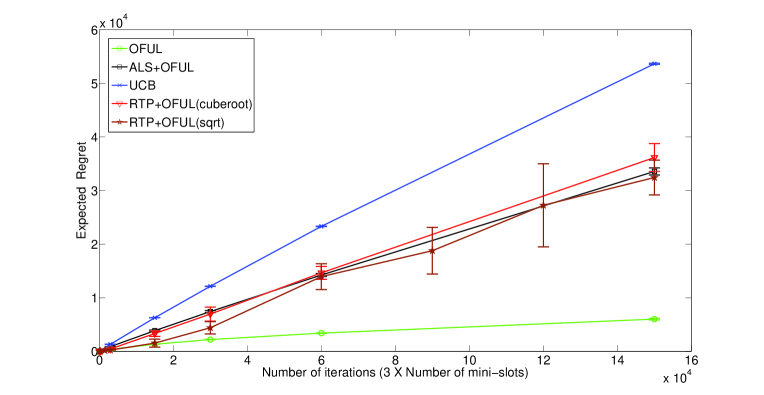
Figure 1: Regret of the proposed algorithm (‘RTP+OFUL’ or Algorithm 3) for two different exploration rate schedules, compared with (a) independent UCB per-user, (b) OFUL per-user with perfect knowledge of latent classes $U$, and (c) Alternating Least Squares estimation for the matrix $U$, along with OFUL per-user. Here, $B=20$ users, $C=3$ classes, and $A=200$, with randomly generated $U$ and $V$. Plots show the sample mean of cumulative regret with time, with $1$ standard deviation-error bars over $10$ sample experiments.

Related work. The popular low-rank matrix completion problem studies the recovery $U$ and $V$ given a small number of entries sampled at random from $UV^{T}$ with both $U$ and $V$ being tall matrices, see for instance Jain et al. (2013) and citations therein. However, its setting is different than ours for several reasons. It typically deals with batch data arising from a sampling process that is not active but uniform across entries of $UV^{T}$. Further, it requires sensing operators having strong properties (such as the RIP property), and most importantly, the performance metric is not regret but reconstruction error (Frobenius or $2$-norm).

In the linear bandit literature (Abbasi-Yadkori et al., 2011; Rusmevichientong and Tsitsiklis, 2010; Dani et al., 2008), the key constraining assumption is that either user side ($V$) or item side ($U$) features are precisely and completely known a priori. In contrast, the problem of low regret recommendation across users with latent mixtures does not afford us the luxury of knowing either $U$ or $V$, and so they must be learnt “on the fly”. Another related work in the context of bandit type schemes for latent mixture model recommender systems is that of Bresler et al. (2014), in which, under the very specific uniform mixture model for all users, they exhibit strategies with good regret.

Nguyen et al. (2014) consider an alternating minimization type scheme in linear bandit models with two-sided uncertainty (an alternative model involving latent “factors”). However no rigorous guarantees are given for the bandit schemes they present; moreover, it is not known if alternating minimization finds global minima in general. Another related work is in the transfer learning setting from Lazaric et al. (2013): The method combines the RTP method (Anandkumar et al., 2014b, 2012) essentially with a standard UCB (Auer et al., 2002), but however works in the setting of a large number interactions with a same user, without assuming access to “user ids”. As a result, the regret bound in this setting scales linearly with the number of rounds. Our result in this paper shows that with additional access to just user identifiers, we can reduce the regret rate to be sublinear in time.

The RTP method has been used as a processing step to the EM algorithm in crowdsourcing (Zhang et al., 2014), but only convergence properties are considered, which is not enough to provide regret guarantees.

On the theoretical side, our contribution generalizes the setting of clustered bandits (Maillard and Mannor, 2014; Gentile et al., 2014) in which a hard clustering model is assumed (one user is assigned to one class, or equivalently mixture distributions can only have support size $1$). In particular, Maillard and Mannor (2014) specifically highlight the benefit of a collaborative gain across users against using a vanilla UCB for each user. However their setting is less general than assuming a soft clustering of users (one user corresponds to a mixture of classes) across various “representative” taste profiles as we study here.

The Alternating Least-Squares (ALS) method (Takács and Tikk, 2012; Mary et al., 2014) has been shown to yield promising experimental results in similar settings where both $U$ and $V$ are unknown. However, no theoretical guarantees are known for this algorithm that may converge to a local optimum in general.

The work of Valko et al. (2014) studies stochastic bandits with a linear model over a low-rank (graph Laplacian) structure. However, they assume complete knowledge of the graph and hence knowledge of the eigenvectors of the Laplacian, converting it into a bilinear problem with only one-sided uncertainty. This is in contrast to our setup where both $U$, $V$ are completely uncertain.

Perhaps the closest work to ours is that of Djolonga et al. (2013) where the authors develop a flexible approach for bandit problems in high dimension but with low-dimensional reward dependence. They use a two-phase algorithm: First a low-rank matrix completion technique (the Dantzig selector) estimates the feature-reward map, then a Gaussian Process-UCB (GP-UCB) bandit algorithm controls the regret, and show that if after $n$ iterations the approximation error between the feature matrix and its estimate is less then $\eta$, the final regret is given by the sum of the regret of GP-UCB when given perfect knowledge of the features and of $n+\eta(T-n)$ (due to the learning phase and approximation error). This results in an overall regret scaling with $O(T^{4/5})$. We depart from their results in two fundamental ways: Firstly, they have the possibility of uniformly sampling the entries (a common assumption in low-rank matrix completion techniques). We do not have this luxury in our setting as we do not control the process of user arrivals, that is not constrained to be uniform. Secondly, we prove and exploit a novel robustness property (see Theorem 8) of the bandit subroutine we use (OFUL in our case instead of GP-UCB), which allows us to effectively eliminate the approximation error in their work and obtain a $O(\sqrt{T})$ regret bound (see Theorem 4).

6 Conclusion & Directions

We consider a full-blown latent class mixture model in which users are described by unknown mixtures across unknown user classes, more general and challenging than when users are assumed to fall perfectly in one class (Gentile et al., 2014; Maillard and Mannor, 2014).

We provide the first provable sublinear regret guarantees in this setting, when both the canonical classes and user mixture weights are completely unknown, which we believe is striking when compared to existing work in the setting, e.g., alternate minimization typically gets stuck in local minima. We currently use a combination of noisy tensor factorization and linear bandit techniques, and control the uncertainty in the estimates resulting from each one of these techniques. This enables us to effectively recover the latent class structure.

Future directions include reducing the numerical constant (e.g. using an alternative to RTP), and studying how to combine our work with the aggregation of user parameters suggested in Maillard and Mannor (2014).

A Proofs of Lemmas 1 and 2

Proof of Lemma 1 This result holds by construction of the estimates $\tilde{r}_{a,a^{\prime},n}$ and $\tilde{r}_{a,a^{\prime},a^{\prime\prime},n}$. Note that

$$\mathbb{E}\big{[}\tilde{r}_{a,a^{\prime},n}\big{]} = \frac{1}{n}\sum_{i=1}^{n}\sum_{b\in[B]}\mathbb{E}\bigg{[}\frac{X_{a_{i,1},b_{i},i,1}X_{a_{i,2},b_{i},i,2}}{p_{i}(a,a^{\prime}|b_{i})}\mathbb{I}\{a_{i,1}=a,a_{i,2}=a^{\prime}\}\bigg{|}b_{i}=b\bigg{]}\beta(b)$$

$$= \frac{1}{n}\sum_{i=1}^{n}\sum_{b\in[B]}\sum_{c\in[C]}\mathbb{E}\bigg{[}\frac{X_{a_{i,1},b,i,1}X_{a_{i,2},b,i,2}}{p_{i}(a,a^{\prime}|b)}\mathbb{I}\{a_{i,1}=a,a_{i,2}=a^{\prime}\}\bigg{|}b_{i}=b,c_{i}=c\bigg{]}v_{b,c}\beta(b)$$

$$= \frac{1}{n}\sum_{i=1}^{n}\sum_{b\in[B]}\sum_{c\in[C]}\mathbb{E}\bigg{[}X_{a,b,i,1}X_{a^{\prime},b,i,2}\bigg{|}b_{i}=b,c_{i}=c\bigg{]}v_{b,c}\beta(b)$$

$$\stackrel{{\scriptstyle(a)}}{{=}} \frac{1}{n}\sum_{i=1}^{n}\sum_{b\in[B]}\sum_{c\in[C]}\mathbb{E}\bigg{[}X_{a,b,i,1}\bigg{|}b_{i}=b,c_{i}=c\bigg{]}\mathbb{E}\bigg{[}X_{a^{\prime},b,i,2}\bigg{|}b_{i}=b,c_{i}=c\bigg{]}v_{b,c}\beta(b)$$

$$= \frac{1}{n}\sum_{i=1}^{n}\sum_{b\in[B]}\sum_{c\in[C]}u_{a,c}u_{a^{\prime},c}v_{b,c}\beta(b)$$

$$= \sum_{c\in[C]}(\sum_{b\in[B]}v_{b,c}\beta(b))u_{a,c}u_{a^{\prime},c}$$

$$= \sum_{c\in[C]}v_{\beta,c}u_{a,c}u_{a^{\prime},c}\,,$$

where $(a)$ holds by independence of the sample generated by user $b$ when in the same class $c$. Note that $c_{i}$ is the same for all $\ell=1,2,3$ interaction steps, that is $c_{i}=c_{i,1}=c_{i,2}=c_{i,3}$, where $c_{i,\ell}$ is the class corresponding to sample $X_{a,b,i,\ell}$. This is the reason why we get $u_{a,c}u_{a^{\prime},c}v_{b,c}$ and not a product $u_{a,c}u_{a^{\prime},c}v_{b,c}^{2}$ for instance.

Proof of Lemma 2 Since the rewards generated by each source $a,b$ are i.i.d., the estimate $\tilde{r}_{a,a^{\prime},n}$ is a sum of i.i.d. random variables bounded in $[0,1]$, re-weighted by the probability weights $p_{i}(a,a^{\prime}|b_{i})$, which are measurable functions of the past. Assuming that there exists some deterministic $q_{2,i}>0$ such that $\forall i\in\mathbb{N},p_{i}(a,a^{\prime}|b_{i})\geqslant q_{2,i}$, we can thus apply a version of Azuma-Hoeffding inequality for bounded martingale difference sequence. Let us recall that by this inequality, for a deterministic time $s$, and $(Y_{m})_{m\leqslant s}\in[0,1]$ being a bounded martingale difference sequence, then for all $\delta\in(0,1)$ it holds

$$\mathbb{P}(|\frac{1}{s}\sum_{i=1}^{s}Y_{i}|\geqslant\sqrt{\frac{\log(2/\delta)}{2s}})\leqslant\delta\,.$$

In our case, $Y_{i}=\frac{X_{a_{i,1},b_{i},i,1}X_{a_{i,2},b_{i},i,2}}{p_{i}(a,a^{\prime}|b_{i})}\mathbb{I}\{a_{i,1}=a,a_{i,2}=a^{\prime}\}-m_{a,a^{\prime}}$, and we deduce that

$$\mathbb{P}(|\tilde{r}_{a,a^{\prime},n}-m_{a,a^{\prime}}|\geqslant\sqrt{\sum_{i=1}^{n}q_{2,i}^{-2}\frac{\log(2/\delta)}{2n^{2}}})\leqslant\delta\,.$$

Likewise, we get that

$$\mathbb{P}(|\tilde{r}_{a,a^{\prime},a^{\prime\prime},n}-m_{a,a^{\prime},a^{\prime\prime}}|\geqslant\sqrt{\sum_{i=1}^{n}q_{3,i}^{-2}\frac{\log(2/\delta)}{2n^{2}}})\leqslant\delta\,.$$

Taking a union bound over the actions in each case, and then over the two events concludes the proof. $\square$

Proof of Corollary 1 From Lemma 2, we deduce that on an event of probability higher than $1-\delta$, it holds simultaneously that

$$e_{n}^{(2)} \stackrel{{\scriptstyle\rm def}}{{=}} \|\widehat{M}_{n,2}-M_{2}\|\leqslant A\sqrt{\sum_{m=1}^{n}q_{2,m}^{-2}\frac{\log(4A^{2}/\delta)}{2n^{2}}})\,\,\text{ and }\,\,$$

$$e_{n}^{(3)} \stackrel{{\scriptstyle\rm def}}{{=}} \|\widehat{M}_{n,3}-M_{3}\|\leqslant A^{3/2}\sqrt{\sum_{m=1}^{n}q_{3,m}^{-2}\frac{\log(4A^{3}/\delta)}{2n^{2}}})\,.$$

This indeed holds by relating the norm of the matrix (tensor) with each of the elements. We conclude by replacing the values of $q_{2,i}$ and $q_{3,i}$.

B Proof of Theorem 1

We prove in this section a slightly more detailed result, namely, the following:

Theorem 1. Assume that $\{\gamma_{i}\}_{i\geqslant 1}$ are chosen such that $n^{-2}\sum_{i=1}^{n}\gamma_{i}^{-2}\stackrel{{\scriptstyle n}}{{\to}}0$. Let $\lambda_{\min}$ be the minimum robust eigenvalue of the tensor $T=M_{3}(W,W,W)$. Let $\delta\in(0,1)$. Provided that

$$\frac{n^{2}}{\sum_{i=1}^{n}\gamma_{i}^{-2}}\geqslant\max\bigg{\{}\frac{2A^{6}\log(4A^{2}/\delta)}{\min\{\Gamma,\sigma_{\min}\}^{2}},\frac{A^{9}(1+10(\frac{1}{\Gamma}+\frac{1}{\sigma_{\min}})(1+u_{\max}^{3}))^{2}C^{5}\log(4A^{3}/\delta)}{2C^{2}_{1}\lambda_{min}^{2}\sigma_{min}^{3}}\bigg{\}}\,,$$

with probability higher than $1-2\delta$, there exists some permutation $\pi\in\mathbb{S}_{C}$ such that for all $c\in[C]$,

$$||u_{c}-\overline{u}_{n,\pi(c)}||\leqslant\Delta A^{3}\sqrt{\sum_{i=1}^{n}\gamma_{i}^{-2}\frac{C\log(4A^{3}/\delta)}{2n^{2}}}+o(n^{-2}\sum_{i=1}^{n}\gamma_{i}^{-2}),$$

where we introduced the problem-dependent constant

$$\Delta = 13\sqrt{\sigma_{max}}\Big{(}\frac{CA}{\sigma_{min}}\Big{)}^{3/2}\Big{(}1+10(\frac{1}{\Gamma}+\frac{1}{\sigma_{\min}})(1+u_{\max}^{3})\Big{)}+\big{(}\frac{2\sigma_{max}}{\Gamma}+\frac{1}{\sigma_{max}}\big{)}\frac{1}{v_{\min}^{2}}\,.$$

For general $\{\gamma_{i}\}_{i\geqslant 1}$ (not necessarily such that $n^{-2}\sum_{i=1}^{n}\gamma_{i}^{-2}\stackrel{{\scriptstyle n}}{{\to}}0$), it holds with same probability that

$$||{\bf u}_{c}-\overline{\bf u}_{n,\pi(c)}||\leqslant\Diamond A^{3}\sqrt{\sum_{i=1}^{n}\gamma_{i}^{-2}\frac{C\log(4A^{3}/\delta)}{2n^{2}}}\,,$$

where, using the notation $\aleph=1+10(\frac{1}{\Gamma}+\frac{1}{\sigma_{\min}})(1+u_{\max}^{3})$, we have introduced the constant

$$\Diamond=\Big{(}\frac{CA}{\sigma_{min}}\Big{)}^{3/2}\bigg{(}13\sqrt{\sigma_{max}}+4\sqrt{2\min\{\Gamma,\sigma_{\min}\}}+5\big{(}\frac{\sigma_{max}}{\Gamma}+\frac{1}{2\sigma_{max}}\big{)}\min\{\Gamma,\sigma_{\min}\}\bigg{)}\aleph$$

$$+\,\,\big{(}\frac{2\sigma_{max}}{\Gamma}+\frac{1}{\sigma_{max}}\big{)}\frac{1}{v_{\min}^{2}}+5\sqrt{3/8}\Big{(}\sqrt{\sigma_{\max}}+\sqrt{\min\{\Gamma,\sigma_{\min}\}/2}\Big{)}\big{(}\frac{2CA}{\sigma_{\min}}\big{)}^{3}\aleph^{2}\min\{\Gamma,\sigma_{\min}\}\,.$$

Proof  The proof closely follows that of Gheshlaghi Azar et al. (2013). First, note that by property of the rank $1$ decomposition ((Anandkumar et al., 2014b, Theorem 4.3)), it holds that $\lambda_{c}=(\sum_{b\in[B]}v_{b,c}\beta(b))^{-2}$ and thus $v_{\min}^{-2}\geqslant\lambda_{\max}\geqslant\lambda_{\min}\geqslant 1$.

We first decompose the following term to make appear the terms from Proposition 1:

$$||{\bf u}_{c}-\overline{{\bf u}}_{n,\pi(c)}||\leqslant$$

$$\underbrace{|\lambda_{c}-\widehat{\lambda}_{n,\pi(c)}|}_{RTP.1}\underbrace{\|{W^{\top}}^{\dagger}\|}_{b}\underbrace{||\varphi_{c}||}_{a}+\underbrace{|\widehat{\lambda}_{\pi(c)}|}_{RTP.3}\underbrace{\|{W^{\top}}^{\dagger}-{\widehat{W}}^{\top}{}^{\dagger}\|}_{d}\underbrace{||\varphi_{c}||}_{1}+\underbrace{|\widehat{\lambda}_{\pi(c)}|}_{RTP.3}\underbrace{\|{\widehat{W}}^{\top}{}^{\dagger}\|}_{c}\underbrace{||\varphi_{c}-\widehat{\varphi}_{n,\pi(c)}||}_{RTP.2}\,.$$

Note that $\varphi_{c}$, and $\widehat{\varphi}_{n,\pi(c)}$ are both normalized vectors. Thus, $(a)$ is bounded as $||\varphi_{c}||\leqslant 1$. It holds for $(b)$ that $\|{W^{\top}}^{\dagger}\|\leqslant\sqrt{C\sigma_{max}}$, and for $(c)$, on the $1-\delta$ event $\Omega$ from Corollary 1, that

$$\|{\widehat{W}}^{\top}{}^{\dagger}\|\leqslant\sqrt{C\widehat{\sigma}_{max}}\leqslant\sqrt{C}(\sqrt{\sigma_{max}}+\sqrt{e_{n}^{(2)}})\,.$$ (4)

The term $(d)$ requires a little more work. It holds that

$$\|{W^{\top}}^{\dagger}-{\widehat{W}}^{\top}{}^{\dagger}\| = \|\widehat{U}\widehat{D}^{1/2}-UD^{1/2}\|$$

$$\leqslant \|(\widehat{U}-U)D^{1/2}\|+\|\widehat{U}(\widehat{D}^{1/2}-D^{1/2})\|$$

$$\leqslant \underbrace{\|\widehat{U}-U\|}_{e}\sigma_{max}+\underbrace{\|\widehat{D}^{1/2}-D^{1/2}\|}_{f}\sqrt{C}\,.$$

We use the result of Lemma 5 from Gheshlaghi Azar et al. (2013) to control $(e)$ and $(f)$. If $e_{n}^{(2)}\leqslant\frac{1}{2}\Gamma$, then it holds

$$\|\widehat{D}^{1/2}-D^{1/2}\|\leqslant\frac{e_{n}^{(2)}}{\sigma_{\max}}\qquad\|\widehat{U}-U\|\leqslant\frac{2\sqrt{C}e_{n}^{(2)}}{\Gamma}\,,$$

from which we deduce that

$$\|{W^{\top}}^{\dagger}-{\widehat{W}}^{\top}{}^{\dagger}\|\leqslant(\frac{2\sigma_{\max}}{\Gamma}+\frac{1}{\sigma_{\max}})\sqrt{C}e_{n}^{(2)}\,.$$ (5)

At this point, $(RTP.1),(RTP.2)$ and $(RTP.3)$ are controlled by the perturbation method from Anandkumar et al. (2014b), under the condition that $e_{n}=\|T-\widehat{T}\|\leqslant C_{1}\frac{\lambda_{min}}{C}$ (where $C_{1}$ is a universal constant). In this case, with probability $1-\delta$, the RTP algorithm with well-chosen parameters achieves

$$|\lambda_{c}-\widehat{\lambda}_{n,\pi(c)}| \leqslant 5\|T-\widehat{T}_{n}\|$$

$$\|\varphi_{c}-\widehat{\varphi}_{n,\pi(c)}\| \leqslant 8\frac{\|T-\widehat{T}_{n}\|}{\lambda_{c}}\,.$$

In order to make the condition explicit in our setting, we use the fact that by Lemma 6 from Gheshlaghi Azar et al. (2013), if $e_{n}^{(2)}\leqslant\frac{1}{2}\min\{\Gamma,\sigma_{\min}\}$ then

$$e_{n}\leqslant\Big{(}\frac{C}{\sigma_{\min}}\Big{)}^{3/2}\bigg{(}e_{n}^{(3)}+2(1+\sqrt{2}+2)e_{n}^{(2)}(\frac{1}{\Gamma_{\sigma}}+\frac{1}{\sigma_{min}})(e_{n}^{(3)}+\max_{c}||{\bf u}_{c}||^{3})\bigg{)}\,.$$ (6)

The condition $e_{n}^{(2)}\leqslant\frac{1}{2}\min\{\Gamma,\sigma_{\min}\}$ holds if the number of sessions $n$ is sufficiently large: Indeed on an event of probability higher than $1-\delta$, then it is enough that

$$A^{3}\sqrt{\sum_{i=1}^{n}\gamma_{i}^{-2}\frac{\log(4A^{2}/\delta)}{2n^{2}}}\leqslant\frac{1}{2}\min\{\Gamma,\sigma_{\min}\}\,,$$

that is, reordering the terms, that

$$\frac{n^{2}}{\sum_{i=1}^{n}\gamma_{i}^{-2}}\geqslant\frac{2A^{6}\log(4A^{2}/\delta)}{\min\{\Gamma,\sigma_{\min}\}^{2}}\,.$$ (7)

Now, in order to satisfy the condition $e_{n}=\|T-\widehat{T}_{n}\|\leqslant C_{1}\frac{\lambda_{\min}}{C}$, it is enough that

$$\Big{(}\frac{C}{\sigma_{\min}}\Big{)}^{3/2}\bigg{(}e_{n}^{(3)}+2(1+\sqrt{2}+2)e_{n}^{(2)}(\frac{1}{\Gamma}+\frac{1}{\sigma_{\min}})(e_{n}^{(3)}+\max_{c}||u_{c}||^{3})\bigg{)}\leqslant C_{1}\frac{\lambda_{\min}}{C}\,.$$

Let us decompose the left-hand-side term: After some simplifications using $\max_{c}||{\bf u}_{c}||^{3}\leqslant A^{3/2}u_{\max}^{3}$ and $e_{n}^{(3)}\leqslant A^{3/2}$, the previous inequality happens when

$$e_{n}^{(3)}+A^{3/2}\varhexagon e_{n}^{(2)}\leqslant C_{1}\frac{\lambda_{min}\sigma_{min}^{3/2}}{C^{5/2}}\,.$$

where $\varhexagon=2(1+\sqrt{2}+2)(\frac{1}{\Gamma}+\frac{1}{\sigma_{\min}})(1+u_{\max}^{3})$. Using the definition of $e_{n}^{(3)}$ and $e_{n}^{(2)}$ then we deduce that it is enough that

$$(1+\varhexagon)A^{9/2}\sqrt{\sum_{i=1}^{n}\gamma_{i}^{-2}\frac{\log(4A^{3}/\delta)}{2n^{2}}}\leqslant C_{1}\frac{\lambda_{min}\sigma_{min}^{3/2}}{C^{5/2}}\,,$$

that is, reordering the terms that

$$\frac{n^{2}}{\sum_{i=1}^{n}\gamma_{i}^{-2}}\geqslant\frac{A^{9}(1+\varhexagon)^{2}C^{5}\log(4A^{3}/\delta)}{2C^{2}_{1}\lambda_{min}^{2}\sigma_{min}^{3}}\,.$$ (8)

Combining the decomposition (B) with (4),(5), and using the fact that $v_{\min}^{-2}\geqslant\lambda_{c}\geqslant 1$, we obtain

$$||{\bf u}_{c}-\bar{\bf u}_{n,\pi(c)}|| \leqslant 5e_{n}\sqrt{C}\sqrt{\sigma_{\max}}+(\lambda_{c}+5e_{n})\sqrt{C}\big{(}\frac{2\sigma_{\max}}{\Gamma}+\frac{1}{\sigma_{\max}}\big{)}e_{n}^{(2)}$$

$$+8\sqrt{C}(\lambda_{c}+5e_{n})(\sqrt{\sigma_{\max}}+\sqrt{e_{n}^{(2)}})\frac{e_{n}}{\lambda_{c}}\,.$$

$$\leqslant \sqrt{C}\bigg{[}13\sqrt{\sigma_{\max}}e_{n}+\big{(}\frac{2\sigma_{\max}}{\Gamma}+\frac{1}{\sigma_{\max}}\big{)}\frac{e_{n}^{(2)}}{v_{\min}^{2}}+8\sqrt{e_{n}^{(2)}}e_{n}$$

$$+5\big{(}\frac{2\sigma_{\max}}{\Gamma}+\frac{1}{\sigma_{\max}}\big{)}e_{n}^{(2)}e_{n}+40(\sqrt{\sigma_{\max}}+\sqrt{e_{n}^{(2)}})e_{n}^{2}\bigg{]}\,.$$

Now, using (6) and unfolding the last inequality, it holds with probability higher than $1-2\delta$ that

$$||{\bf u}_{c}-\bar{\bf u}_{n,\pi(c)}||$$

$$\leqslant \sqrt{C}\bigg{[}13\sqrt{\sigma_{max}}\Big{(}\frac{C}{\sigma_{min}}\Big{)}^{3/2}(e_{n}^{(3)}+e_{n}^{(2)}A^{3/2}\varhexagon)+\big{(}\frac{2\sigma_{max}}{\Gamma_{\sigma}}+\frac{1}{\sigma_{max}}\big{)}\frac{e_{n}^{(2)}}{v_{\min}^{2}}$$

$$+8\Big{(}\frac{C}{\sigma_{min}}\Big{)}^{3/2}\sqrt{e_{n}^{(2)}}(e_{n}^{(3)}+e_{n}^{(2)}A^{3/2}\varhexagon)$$

$$+5\Big{(}\frac{C}{\sigma_{min}}\Big{)}^{3/2}\big{(}\frac{2\sigma_{max}}{\Gamma_{\sigma}}+\frac{1}{\sigma_{max}}\big{)}e_{n}^{(2)}(e_{n}^{(3)}+e_{n}^{(2)}A^{3/2}\varhexagon)+40(\sqrt{\sigma_{max}}+\sqrt{e_{n}^{(2)}})e_{n}^{2}\bigg{]}$$

$$\leqslant \bigg{[}13\sqrt{\sigma_{max}}\Big{(}\frac{CA}{\sigma_{min}}\Big{)}^{3/2}(1+\varhexagon)+\big{(}\frac{2\sigma_{max}}{\Gamma_{\sigma}}+\frac{1}{\sigma_{max}}\big{)}\frac{1}{v_{\min}^{2}}\bigg{]}$$

$$\times A^{3}\sqrt{\sum_{i=1}^{n}\gamma_{i}^{-2}\frac{C\log(4A^{3}/\delta)}{2n^{2}}}+o(n^{-2}\sum_{i=1}^{n}\gamma_{i}^{-2})\,,$$

which, after some cosmetic simplifications, concludes the first part of the proof of Theorem 1.

Alternatively, when $n^{-2}\sum_{i=1}^{n}\gamma_{i}^{-2}\not\to\infty$, we can always resort to the condition that $e_{n}^{(2)}\leqslant 1/2\min\{\Gamma,\sigma_{\min}\}$ in order to simplify the previous derivation. We deduce, similarly, that

$$||{\bf u}_{c}-\bar{\bf u}_{n,\pi(c)}||$$

$$\leqslant \sqrt{C}\bigg{[}13\sqrt{\sigma_{max}}\Big{(}\frac{C}{\sigma_{min}}\Big{)}^{3/2}(e_{n}^{(3)}+e_{n}^{(2)}A^{3/2}\varhexagon)+\big{(}\frac{2\sigma_{max}}{\Gamma_{\sigma}}+\frac{1}{\sigma_{max}}\big{)}\frac{e_{n}^{(2)}}{v_{\min}^{2}}$$

$$+8\Big{(}\frac{C}{\sigma_{min}}\Big{)}^{3/2}\sqrt{e_{n}^{(2)}}(e_{n}^{(3)}+e_{n}^{(2)}A^{3/2}\varhexagon)$$

$$+5\Big{(}\frac{C}{\sigma_{min}}\Big{)}^{3/2}\big{(}\frac{2\sigma_{max}}{\Gamma_{\sigma}}+\frac{1}{\sigma_{max}}\big{)}e_{n}^{(2)}(e_{n}^{(3)}+e_{n}^{(2)}A^{3/2}\varhexagon)+40(\sqrt{\sigma_{max}}+\sqrt{e_{n}^{(2)}})e_{n}^{2}\bigg{]}$$

$$\leqslant \bigg{[}\bigg{(}13\sqrt{\sigma_{max}}\Big{(}\frac{CA}{\sigma_{min}}\Big{)}^{3/2}+8\Big{(}\frac{CA}{\sigma_{min}}\Big{)}^{3/2}\sqrt{\min\{\Gamma,\sigma_{\min}\}/2}$$

$$+5\Big{(}\frac{CA}{\sigma_{min}}\Big{)}^{3/2}\big{(}\frac{\sigma_{max}}{\Gamma_{\sigma}}+\frac{1}{2\sigma_{max}}\big{)}\min\{\Gamma,\sigma_{\min}\}\bigg{)}(1+\varhexagon)+\big{(}\frac{2\sigma_{max}}{\Gamma_{\sigma}}+\frac{1}{\sigma_{max}}\big{)}\frac{1}{v_{\min}^{2}}$$

$$+40\Big{(}\sqrt{\sigma_{\max}}+\sqrt{\min\{\Gamma,\sigma_{\min}\}/2}\Big{)}\big{(}\frac{CA}{\sigma_{\min}}\big{)}^{3}(1+\varhexagon)^{2}\min\{\Gamma,\sigma_{\min}\}\sqrt{3/8}\bigg{]}$$

$$\times A^{3}\sqrt{\sum_{i=1}^{n}\gamma_{i}^{-2}\frac{C\log(4A^{3}/\delta)}{2n^{2}}}\,,$$

where, in order to control the last term $e_{n}^{2}$, we used the property that

$$e_{n} \leqslant \Big{(}\frac{CA}{\sigma_{\min}}\Big{)}^{3/2}\Big{(}1+\varhexagon\Big{)}\min\{e_{n}^{(2)}\sqrt{\frac{\log(4A^{3}/\delta)}{\log(4A^{2}/\delta)}},A^{-3/2}e_{n}^{(3)}\}$$

$$\leqslant \Big{(}\frac{CA}{\sigma_{\min}}\Big{)}^{3/2}\Big{(}1+\varhexagon\Big{)}\min\{\sqrt{3/2}e_{n}^{(2)},A^{-3/2}e_{n}^{(3)}\}\,.$$

 

C Proof of Theorem 3

Proof  Let $\mathbf{M}_{1:t}=({\bf m}_{A_{1}},\ldots,{\bf m}_{A_{t}})^{\top}$. The argument used to prove Theorem 2 in Yadkori et al, 2011, can be used to show that

$$\widehat{\bf v}_{t-1} =V_{t-1}^{-1}\bar{\bf U}_{1:t-1}\eta_{1:t-1}+V_{t-1}^{-1}\bar{\bf U}_{1:t-1}\mathbf{M}_{1:t-1}$$

where $\eta_{1:t-1}:=(\eta_{1},\ldots,\eta_{t-1})$ is the observed noise sequence. Let $\mathbf{E}_{1:t-1}:=(\varepsilon_{A_{1}},\ldots,\varepsilon_{A_{t}})^{\top}=\mathbf{M}_{1:t-1}-\bar{\bf U}_{1:t-1}{\bf v}^{\circ}$. We then have

$$\widehat{\bf v}_{t-1} =V_{t-1}^{-1}\bar{\bf U}_{1:t-1}\eta_{1:t-1}+V_{t-1}^{-1}\bar{\bf U}_{1:t-1}\mathbf{M}_{1:t-1}$$

$$=V_{t-1}^{-1}\bar{\bf U}_{1:t-1}\eta_{1:t-1}+V_{t-1}^{-1}\bar{\bf U}_{1:t-1}\left(\bar{\bf U}_{1:t-1}^{\top}{\bf v}^{\circ}+\mathbf{E}_{1:t-1}\right)$$

$$=V_{t-1}^{-1}\bar{\bf U}_{1:t-1}\eta_{1:t-1}+{\bf v}^{\circ}-\lambda V_{t-1}^{-1}{\bf v}^{\circ}+V_{t-1}^{-1}\bar{\bf U}_{1:t-1}\mathbf{E}_{1:t-1}.$$

Thus, letting ${\bf v}_{t-1}^{+}:={\bf v}^{\circ}+V_{t-1}^{-1}\bar{U}_{1:t-1}\mathbf{E}_{1:t-1}$ and using the above with techniques from Yadkori et al together with $\left\lVert{\bf v}^{\circ}\right\rVert_{2}\leqslant R_{\Theta}$, we have that

$${\bf v}_{t-1}^{+}\in\mathcal{C}_{t-1}$$

with probability at least $1-\delta$.

Now, let $a_{t-1}^{+}\in\arg\max_{a\in\mathcal{A}}\bar{\bf u}_{a}^{\top}{\bf v}_{t-1}^{+}$ be an optimal action corresponding to the approximate parameter ${\bf v}_{t-1}^{+}$, and define the instantaneous regret at time $t$ with respect to the approximate parameter as

$$r_{t}^{+}:=\bar{\bf u}_{a_{t-1}^{+}}^{\top}{\bf v}_{t-1}^{+}-\bar{\bf u}_{A_{t}}^{\top}{\bf v}_{t-1}^{+}\geqslant 0.$$

We now bound this approximate regret using arguments along the lines of Yadkori et al, 2011. Consider

$$r_{t}^{+} =\bar{\bf u}_{a_{t-1}^{+}}^{\top}{\bf v}_{t-1}^{+}-\bar{\bf u}_{A_{t}}^{\top}{\bf v}_{t-1}^{+}$$

$$\leqslant\bar{\bf u}_{A_{t}}^{\top}\tilde{{\bf v}}_{t}-\bar{\bf u}_{A_{t}}^{\top}{\bf v}_{t-1}^{+}\quad\quad\mbox{(since $(A_{t},\tilde{{\bf v}}_{t})$ is optimistic)}$$

$$=\bar{\bf u}_{A_{t}}^{\top}\left(\tilde{{\bf v}}_{t}-{\bf v}_{t-1}^{+}\right)$$

$$=\bar{\bf u}_{A_{t}}^{\top}\left(\tilde{{\bf v}}_{t}-\widehat{{\bf v}}_{t-1}\right)+\bar{\bf u}_{A_{t}}^{\top}\left(\widehat{{\bf v}}_{t-1}-{\bf v}_{t-1}^{+}\right)$$

$$\leqslant\left\lVert\bar{\bf u}_{A_{t}}\right\rVert_{V_{t-1}^{-1}}\left\lVert\tilde{{\bf v}}_{t}-\widehat{{\bf v}}_{t-1}\right\rVert_{V_{t-1}}+\left\lVert\bar{\bf u}_{A_{t}}\right\rVert_{V_{t-1}^{-1}}\left\lVert\widehat{{\bf v}}_{t-1}-{\bf v}_{t-1}^{+}\right\rVert_{V_{t-1}}\quad\quad\mbox{(Cauchy-Schwarz's inequality)}$$

$$\leqslant 2{D_{t-1}}\left\lVert\bar{\bf u}_{A_{t}}\right\rVert_{V_{t-1}^{-1}}.$$ (9)

Noting that $m_{a}\in[-1,1]$ $\forall a$, the regret can be written as

$$R_{T} =\sum_{t=1}^{T}\left(m_{a^{\star}}-m_{A_{t}}\right)=\sum_{t=1}^{T}\min\{m_{a^{\star}}-m_{A_{t}},2\}$$

$$=\rho^{\prime}\sum_{a\neq a^{\star}}\sum_{t=1}^{T}\min\left\{\frac{m_{a^{\star}}-m_{a}}{\rho^{\prime}},\frac{2}{\rho^{\prime}}\right\}\mathbb{I}\{A_{t}=a\}$$

$$\leqslant\rho^{\prime}\sum_{a\neq a^{\star}}\sum_{t=1}^{T}\min\left\{\bar{\bf u}_{a^{\star}}^{\top}{\bf v}^{\circ}-\bar{\bf u}_{a}^{\top}{\bf v}^{\circ},\frac{2}{\rho^{\prime}}\right\}\mathbb{I}\{A_{t}=a\}\quad\mbox{(using the definition of $\rho^{\prime}$)}$$

$$\stackrel{{\scriptstyle(a)}}{{\leqslant}}\rho^{\prime}\sum_{t=1}^{T}\min\left\{2\left(\bar{\bf u}_{a^{\star}}^{\top}{\bf v}_{t-1}^{+}-\bar{\bf u}_{A_{t}}^{\top}{\bf v}_{t-1}^{+}\right),\frac{2}{\rho^{\prime}}\right\}\stackrel{{\scriptstyle(b)}}{{=}}2\rho^{\prime}\sum_{t=1}^{T}\min\left\{\bar{\bf u}_{a_{t-1}^{+}}^{\top}{\bf v}_{t-1}^{+}-\bar{\bf u}_{A_{t}}^{\top}{\bf v}_{t-1}^{+},\frac{1}{\rho^{\prime}}\right\}$$

$$=2\rho^{\prime}\sum_{t=1}^{T}\min\left\{r_{t}^{+},\frac{1}{\rho^{\prime}}\right\}=\rho^{\prime}\sum_{t=1}^{T}\frac{2}{\rho^{\prime}}\min\left\{{\rho^{\prime}r_{t}^{+}},1\right\}\stackrel{{\scriptstyle(c)}}{{\leqslant}}\rho^{\prime}\sum_{t=1}^{T}\frac{2}{\rho^{\prime}}\min\left\{2\rho^{\prime}{D_{t-1}}\left\lVert\bar{\bf u}_{A_{t}}\right\rVert_{V_{t-1}^{-1}},1\right\}$$

$$\stackrel{{\scriptstyle(d)}}{{\leqslant}}\rho^{\prime}\sum_{t=1}^{T}{4}D_{t-1}\min\left\{\left\lVert\bar{\bf u}_{A_{t}}\right\rVert_{V_{t-1}^{-1}},1\right\}$$

$$\leqslant\rho^{\prime}\sqrt{T\sum_{t=1}^{T}16{D_{T}}^{2}\min\left\{\left\lVert\bar{\bf u}_{A_{t}}\right\rVert_{V_{t-1}^{-1}}^{2},1\right\}}\quad\mbox{(by using Cauchy-Schwarz's inequality)}.$$

In the derivation above,

• Steps $(a)$ and $(b)$ hold because of the following. By Lemma 4 (to follow below), $\left\lVert{\bf v}_{t-1}^{+}-{\bf v}^{\circ}\right\rVert_{2}=\left\lVert V_{t-1}^{-1}\bar{\bf U}_{1:t-1}\mathbf{E}_{1:t-1}\right\rVert_{2}\leqslant\alpha(\bar{U})\left\lVert\varepsilon\right\rVert_{2}$. Since $\arg\max_{a\in\mathcal{A}}\bar{\bf u}_{a}^{\top}{\bf v}^{\circ}$ is uniquely $a^{\star}$ by hypothesis, we have, thanks to Lemma 5 (to follow below), that $\bar{\bf u}_{a^{\star}}^{\top}{\bf v}_{t-1}^{+}-\bar{\bf u}_{a}^{\top}{\bf v}_{t-1}^{+}>\frac{\bar{\bf u}_{a^{\star}}^{\top}{\bf v}^{\circ}-\bar{\bf u}_{a}^{\top}{\bf v}^{\circ}}{2}>0$ $\forall a\neq a^{\star}$, establishing $(a)$. This in turn shows that the optimal action for ${\bf v}_{t-1}^{+}$ is uniquely $a^{\star}$ at all times $t$, i.e., $a_{t-1}^{+}=\arg\max_{a\in\mathcal{A}}\bar{\bf u}_{a}^{\top}{\bf v}_{t-1}^{+}=a^{\star}$, which is equality $(b)$.

• Inequality $(c)$ holds by (9) and $(d)$ holds because $\rho^{\prime}\geqslant 1$ by definition, and $D_{t-1}\geqslant\lambda^{1/2}R_{\Theta}\geqslant 1/2$ by hypothesis, implying that $2\rho^{\prime}D_{t-1}\geqslant 1$.

The argument from here can be continued in the same way as in Abbasi-Yadkori et al. (2011) to yield

$$R_{T}\leqslant 8\rho^{\prime}\sqrt{TC\log\left(1+\frac{TR_{\mathcal{X}}^{2}}{\lambda C}\right)}\left(\lambda^{1/2}R_{\Theta}+R\sqrt{2\log\frac{1}{\delta}+C\log\left(1+\frac{TR_{\mathcal{X}}^{2}}{\lambda C}\right)}\right).$$

This proves the theorem.

 

Lemma 4 (Analysis of the time-varying parameter error $V_{t-1}^{-1}\bar{\bf U}_{1:t-1}\mathbf{E}_{1:t-1}$)

Let $\varepsilon_{a}=m_{a}-\bar{\bf u}_{a}^{\top}{\bf v}^{\circ}$ be the bias in arm $a$’s reward due to model error, and let $\varepsilon\equiv(\varepsilon_{a})_{a\in\mathcal{A}}$ be the $|\mathcal{A}|$ dimensional vector of arm reward biases. Then,

$$\left\lVert V_{t-1}^{-1}\bar{\bf U}_{1:t-1}\mathbf{E}_{1:t-1}\right\rVert_{2}\leqslant\left(\max_{J}\left\lVert\mathbf{A}_{J}^{-1}\right\rVert_{2}\right)\left\lVert\varepsilon\right\rVert_{2},$$

where $\mathbf{A}_{(A+C)\times C}=\left[\begin{array}[]{c}\bar{U}\\ I_{d}\end{array}\right]$, $\mathbf{A}_{J}$ is the $C\times C$ submatrix of $\mathbf{A}$ formed by picking rows $J$, and $J$ ranges over all subsets of full-rank rows of $\mathbf{A}$.

Proof [Proof of Lemma 4] Let $z_{t-1}:=V_{t-1}^{-1}\bar{\bf U}_{1:t-1}\mathbf{E}_{1:t-1}={\bf v}_{t-1}-{\bf v}^{\circ}\in\mathbb{R}^{C}$, with $\left\lVert{\bf E}_{1:t-1}\right\rVert_{\infty}\leqslant\left\lVert\varepsilon\right\rVert_{\infty}=\left\lVert{\bf m}-\bar{U}{\bf v}^{\circ}\right\rVert_{\infty}$. We have

$$z_{t-1} =\left(\sum_{s=1}^{t-1}\bar{\bf u}_{A_{s}}\bar{\bf u}_{A_{s}}^{\top}+\lambda I\right)^{-1}\sum_{s=1}^{t-1}\varepsilon_{A_{s}}\bar{\bf u}_{A_{s}}$$

$$=\left(\frac{1}{t-1}\sum_{s=1}^{t-1}\bar{\bf u}_{A_{s}}\bar{\bf u}_{A_{s}}^{\top}+\frac{\lambda}{t-1}I\right)^{-1}\frac{1}{t-1}\sum_{s=1}^{t-1}\varepsilon_{A_{s}}\bar{\bf u}_{A_{s}}$$

$$=\left(\sum_{a\in\mathcal{A}}\bar{\bf u}_{a}\bar{\bf u}_{a}^{\top}\frac{\sum_{s=1}^{t-1}\mathbb{I}\{A_{s}=a\}}{t-1}+\frac{\lambda}{t-1}I\right)^{-1}\sum_{a\in\mathcal{A}}\varepsilon_{a}\bar{\bf u}_{a}\frac{\sum_{s=1}^{t-1}\mathbb{I}\{A_{s}=a\}}{t-1}$$

$$=\left(\sum_{a\in\mathcal{A}}\bar{\bf u}_{a}\bar{\bf u}_{a}^{\top}f_{a}(t-1)+\frac{\lambda}{t-1}I\right)^{-1}\sum_{a\in\mathcal{A}}\varepsilon_{a}\bar{\bf u}_{a}f_{a}(t-1),$$

where $f_{a}(t-1)\equiv f_{a}$ represents the empirical frequency with which action $a\in\mathcal{A}$ has been played up to and including time $t-1$. This allows us to equivalently interpret $z_{t-1}$ as the solution of a weighted $\ell^{2}$-regularized least squares regression problem with $K=|\mathcal{A}|$ observations (instead of the original interpretation with $t-1$ observations) as follows.

Let $\mathbf{F}^{1/2}$ be the $A\times A$ diagonal matrix with the values $\sqrt{f_{1}},\ldots,\sqrt{f_{A}}$ on the diagonal (note: $\sum_{a=1}^{A}f_{a}=1$). With this, we can express $z_{t-1}$ as

$$z_{t-1} =\arg\min_{z\in\mathbb{R}^{C}}\left\lVert\mathbf{F}^{1/2}\bar{U}z-\mathbf{F}^{1/2}\varepsilon\right\rVert_{2}^{2}+\frac{\lambda}{t-1}\left\lVert z\right\rVert_{2}^{2}$$

$$=\arg\min_{z\in\mathbb{R}^{C}}\left\lVert\mathbf{F}^{1/2}\left(\bar{U}z-\varepsilon\right)\right\rVert_{2}^{2}+\frac{\lambda}{t-1}\left\lVert z\right\rVert_{2}^{2}$$

$$=\arg\min_{z\in\mathbb{R}^{C}}\left\lVert\left[\begin{array}[]{cc}\mathbf{F}^{1/2}&0\\ 0&\sqrt{\frac{\lambda}{t-1}}I_{C}\end{array}\right]\left(\left[\begin{array}[]{c}\bar{U}\\ I_{C}\end{array}\right]z-\left[\begin{array}[]{c}\varepsilon\\ 0\end{array}\right]\right)\right\rVert_{2}^{2}$$

$$\equiv\arg\min_{z\in\mathbb{R}^{C}}\left\lVert\mathbf{D}^{1/2}\left(\mathbf{A}z-\mathbf{b}\right)\right\rVert_{2}^{2}=(\mathbf{A}^{\top}\mathbf{D}\mathbf{A})^{-1}\mathbf{A}^{\top}\mathbf{D}\mathbf{b},$$

with $\mathbf{D}^{1/2}$ being a $(A+C)\times(A+C)$ diagonal & positive semidefinite matrix, $\mathbf{A}^{\top}\mathbf{D}\mathbf{A}=\sum_{a\in\mathcal{A}}\bar{\bf u}_{a}\bar{\bf u}_{a}^{\top}f_{a}(t-1)+\frac{\lambda}{t-1}I$ positive definite, and $\mathbf{A}$ having full column rank $C$. A result of Forsgren (1996, Corollary 2.3) can now be applied to yield

$$\left\lVert(\mathbf{A}^{\top}\mathbf{D}\mathbf{A})^{-1}\mathbf{A}^{\top}\mathbf{D}\right\rVert_{2} \leqslant\max_{J}\left\lVert\mathbf{A}_{J}^{-1}\right\rVert_{2}$$

where $J$ ranges over all subsets of full-rank rows of $\mathbf{A}$, and $\mathbf{A}_{J}$ is the $C\times C$ submatrix of $\mathbf{A}$ formed by picking rows $J$. Thus, $\left\lVert z_{t-1}\right\rVert_{2}\leqslant\left(\max_{J}\left\lVert\mathbf{A}_{J}^{-1}\right\rVert_{2}\right)\left\lVert\varepsilon\right\rVert_{2}$. This proves the lemma.  

Lemma 5 (Critical radius)

Let $\bar{\bf u}_{a^{\star}}^{\top}{\bf v}^{\circ}>\bar{\bf u}_{a}^{\top}{\bf v}^{\circ}$ $\forall a\neq a^{\star}$. Then, the following are equivalent:

$$\left\lVert{\bf v}-{\bf v}^{\circ}\right\rVert_{2}\leqslant\alpha(\bar{U})\left\lVert\varepsilon\right\rVert_{2}\;\Rightarrow\;\bar{\bf u}_{a^{\star}}^{\top}{\bf v}-\bar{\bf u}_{a}^{\top}{\bf v}>\frac{\bar{\bf u}_{a^{\star}}^{\top}{\bf v}^{\circ}-\bar{\bf u}_{a}^{\top}{\bf v}^{\circ}}{2}\quad\forall a\neq a^{\star},$$ (10)

and

$$\left\lVert\varepsilon\right\rVert_{2}<\min_{a\neq a^{\star}}\;\frac{\bar{\bf u}_{a^{\star}}^{\top}{\bf v}^{\circ}-\bar{\bf u}_{a}^{\top}{\bf v}^{\circ}}{2\alpha(\bar{U})\left\lVert\bar{\bf u}_{a^{\star}}-\bar{\bf u}_{a}\right\rVert_{2}}.$$ (11)

Proof [Proof of Lemma 5] Assuming (11), observe that when ${\bf v}$ lies in the interior of an $\alpha(\bar{U})\left\lVert\varepsilon\right\rVert_{2}$-ball around ${\bf v}^{\circ}$, we have, for any $a\neq a^{\star}$,

$$\left(\bar{\bf u}_{a^{\star}}-\bar{\bf u}_{a}\right)^{\top}{\bf v} =\left(\bar{\bf u}_{a^{\star}}-\bar{\bf u}_{a}\right)^{\top}{\bf v}^{\circ}+\left(\bar{\bf u}_{a^{\star}}-\bar{\bf u}_{a}\right)^{\top}\left({\bf v}-{\bf v}^{\circ}\right)$$

$$\geqslant\left(\bar{\bf u}_{a^{\star}}-\bar{\bf u}_{a}\right)^{\top}{\bf v}^{\circ}+\min_{\left\lVert\psi\right\rVert_{2}\leqslant\alpha(\bar{U})\left\lVert\varepsilon\right\rVert_{2}}\left(\bar{\bf u}_{a^{\star}}-\bar{\bf u}_{a}\right)^{\top}\psi$$

$$=\left(\bar{\bf u}_{a^{\star}}-\bar{\bf u}_{a}\right)^{\top}{\bf v}^{\circ}-{\alpha(\bar{U})\left\lVert\varepsilon\right\rVert_{2}}{\left\lVert\bar{\bf u}_{a^{\star}}-\bar{\bf u}_{a}\right\rVert_{2}}$$

$$>\left(\bar{\bf u}_{a^{\star}}-\bar{\bf u}_{a}\right)^{\top}{\bf v}^{\circ}-{\alpha(\bar{U})}{\left\lVert\bar{\bf u}_{a^{\star}}-\bar{\bf u}_{a}\right\rVert_{2}}\frac{\bar{\bf u}_{a^{\star}}^{\top}{\bf v}^{\circ}-\bar{\bf u}_{a}^{\top}{\bf v}^{\circ}}{2\alpha(\bar{U})\left\lVert\bar{\bf u}_{a^{\star}}-\bar{\bf u}_{a}\right\rVert_{2}}$$

$$=\frac{\bar{\bf u}_{a^{\star}}^{\top}{\bf v}^{\circ}-\bar{\bf u}_{a}^{\top}{\bf v}^{\circ}}{2},$$

which proves one direction of the lemma. For the other direction, note that if $\left\lVert\varepsilon\right\rVert_{2}\geqslant\frac{\bar{\bf u}_{a^{\star}}^{\top}{\bf v}^{\circ}-\bar{\bf u}_{a}^{\top}{\bf v}^{\circ}}{2\alpha(\bar{U})\left\lVert\bar{\bf u}_{a^{\star}}-\bar{\bf u}_{a}\right\rVert_{2}}$ for some $a\neq a^{\star}$, then by setting ${\bf v}={\bf v}^{\circ}-\frac{\left(\bar{\bf u}_{a^{\star}}^{\top}{\bf v}^{\circ}-\bar{\bf u}_{a}^{\top}{\bf v}^{\circ}\right)(\bar{\bf u}_{a^{\star}}-\bar{\bf u}_{a})}{2\left\lVert\bar{\bf u}_{a^{\star}}-\bar{\bf u}_{a}\right\rVert_{2}^{2}}$, we have both

$$\left\lVert{\bf v}-{\bf v}^{\circ}\right\rVert_{2} =\left\lVert\frac{\left(\bar{\bf u}_{a^{\star}}^{\top}{\bf v}^{\circ}-\bar{\bf u}_{a}^{\top}{\bf v}^{\circ}\right)(\bar{\bf u}_{a^{\star}}-\bar{\bf u}_{a})}{2\left\lVert\bar{\bf u}_{a^{\star}}-\bar{\bf u}_{a}\right\rVert_{2}^{2}}\right\rVert_{2}=\frac{\bar{\bf u}_{a^{\star}}^{\top}{\bf v}^{\circ}-\bar{\bf u}_{a}^{\top}{\bf v}^{\circ}}{2\left\lVert\bar{\bf u}_{a^{\star}}-\bar{\bf u}_{a}\right\rVert_{2}}\leqslant\alpha(\bar{U})\left\lVert\varepsilon\right\rVert_{2}$$

and

$$\left(\bar{\bf u}_{a^{\star}}-\bar{\bf u}_{a}\right)^{\top}{\bf v} =\left(\bar{\bf u}_{a^{\star}}-\bar{\bf u}_{a}\right)^{\top}{\bf v}^{\circ}-\left(\bar{\bf u}_{a^{\star}}-\bar{\bf u}_{a}\right)^{\top}\frac{\left(\bar{\bf u}_{a^{\star}}^{\top}{\bf v}^{\circ}-\bar{\bf u}_{a}^{\top}{\bf v}^{\circ}\right)(\bar{\bf u}_{a^{\star}}-\bar{\bf u}_{a})}{2\left\lVert\bar{\bf u}_{a^{\star}}-\bar{\bf u}_{a}\right\rVert_{2}^{2}}=\frac{\left(\bar{\bf u}_{a^{\star}}-\bar{\bf u}_{a}\right)^{\top}{\bf v}^{\circ}}{2}$$

which contradicts (10), and we are done.  

C.1 Proof of Lemma 3

We begin by establishing some auxiliary technical results, which together imply Lemma 3.

Lemma 6 (Controlling $\alpha_{n}$)

If $n$ is large enough so that (1) and

$$\Diamond A^{3}C\sqrt{\sum_{i=1}^{n}\gamma_{i}^{-2}\frac{\log(4A^{3}/\delta)}{2n^{2}}}\leqslant\frac{1}{2\alpha_{\star}},$$ (12)

hold, then with probability at least $1-\delta$,

$$\alpha_{n}\leqslant 2\alpha_{\star}.$$ (13)

Proof [Proof of Lemma 6] The first step is to estimate the factor $\alpha$ in the analysis of Perturbed OFUL. Towards this, note that the quantity $\alpha\equiv\alpha(\bar{U})$ in our setting becomes

$$\alpha_{n}\equiv\alpha_{n}(\bar{U}_{n})=\max_{J}\left\lVert(u^{\diamond}_{n})_{J}^{-1}\right\rVert_{2},$$

where $u^{\diamond}_{n}:=\left[\begin{array}[]{c}\bar{U}_{n}\\ I_{C}\end{array}\right]$ has rank $C$, and $J$ ranges over all combinations of its $C$ full-rank rows. For any such subset of $C$ linearly independent rows $J$, we have, after denoting $u^{\diamond}:=\left[\begin{array}[]{c}U\\ I_{C}\end{array}\right]$, that

$$\left\lVert(u^{\diamond}_{n})_{J}^{-1}\right\rVert_{2} \leqslant\left\lVert(u^{\diamond})_{J}^{-1}\right\rVert_{2}+\left\lVert(u^{\diamond}_{n})_{J}^{-1}-(u^{\diamond})_{J}^{-1}\right\rVert_{2}.$$

The final term above can be bounded using Anandkumar et al. (2012, Lemma E.4) – a version of Theorem 2.5 in Stewart et al. (1990). Assuming $(u^{\diamond})_{J}$ is invertible, and $\left\lVert(u^{\diamond})_{J}^{-1}\left((u^{\diamond}_{n})_{J}-(u^{\diamond})_{J}\right)\right\rVert_{2}<1$, then $(u^{\diamond}_{n})_{J}$ is invertible, and a resulting bound on the norm of its inverse lets us write

$$\left\lVert(u^{\diamond})_{J}^{-1}\right\rVert_{2}+\left\lVert(u^{\diamond}_{n})_{J}^{-1}-(u^{\diamond})_{J}^{-1}\right\rVert_{2} \leqslant\left\lVert(u^{\diamond})_{J}^{-1}\right\rVert_{2}+\frac{\left\lVert(u^{\diamond}_{n})_{J}-(u^{\diamond})_{J}\right\rVert_{2}\left\lVert(u^{\diamond})_{J}^{-1}\right\rVert_{2}^{2}}{1-\left\lVert(u^{\diamond})_{J}^{-1}\left((u^{\diamond}_{n})_{J}-(u^{\diamond})_{J}\right)\right\rVert_{2}}.$$

Writing $J=J_{u}\cup J_{l}$ ($u$ and $l$ stand for “upper” and “lower”) with $J_{l}$ representing the subset of rows taken from the bottom $C$ rows of $u^{\diamond}_{n}$ (i.e., $I_{C}$), we have

$$(u^{\diamond}_{n})_{J}-(u^{\diamond})_{J}=\left[\begin{array}[]{c}(\bar{U}_{n}-U)_{J_{u}}\\ 0\end{array}\right].$$

Thus, with $\left\lVert\cdot\right\rVert_{F}$ denoting the Frobenius norm, and using the dominance of the Frobenius norm over the matrix $2$-norm, with probability at least $1-\delta$,

$$\left\lVert(u^{\diamond}_{n})_{J}-(u^{\diamond})_{J}\right\rVert_{2} \leqslant\left\lVert(u^{\diamond}_{n})_{J}-(u^{\diamond})_{J}\right\rVert_{F}=\left\lVert(\bar{U}_{n}-U)_{J_{u}}\right\rVert_{F}\leqslant\left\lVert\bar{U}_{n}-U\right\rVert_{F}$$

$$=\sqrt{\sum_{c\in[C]}\left\lVert\bar{U}_{n,c}-U_{c}\right\rVert_{2}^{2}}$$

$$\leqslant\Diamond A^{3}C\sqrt{\sum_{i=1}^{n}\gamma_{i}^{-2}\frac{\log(4A^{3}/\delta)}{2n^{2}}},$$ (14)

from the RTP error estimate (1).

Now, letting $\alpha\equiv\alpha(U)=\max_{J}\left\lVert\left(u^{\diamond}_{J}\right)^{-1}\right\rVert_{2}$, the result above implies that for any suitable $J$,

$$\left\lVert(u^{\diamond})_{J}^{-1}\left((u^{\diamond}_{n})_{J}-(u^{\diamond})_{J}\right)\right\rVert_{2} \leqslant\left\lVert(u^{\diamond})_{J}^{-1}\right\rVert_{2}\left\lVert(u^{\diamond}_{n})_{J}-(u^{\diamond})_{J}\right\rVert_{2}$$

$$\leqslant\alpha\left\lVert(u^{\diamond}_{n})_{J}-(u^{\diamond})_{J}\right\rVert_{2}$$

$$\leqslant\alpha\Diamond A^{3}C\sqrt{\sum_{i=1}^{n}\gamma_{i}^{-2}\frac{\log(4A^{3}/\delta)}{2n^{2}}}$$

$$<1/2$$

whenever $n$ is large enough to satisfy (12).

When the condition (12) above holds, we get, for any $J$ at time $n$,

$$\left\lVert(u^{\diamond}_{n})_{J}^{-1}\right\rVert_{2} \leqslant\left\lVert(u^{\diamond})_{J}^{-1}\right\rVert_{2}+\frac{\left\lVert(u^{\diamond}_{n})_{J}-(u^{\diamond})_{J}\right\rVert_{2}\left\lVert(u^{\diamond})_{J}^{-1}\right\rVert_{2}^{2}}{1-\left\lVert(u^{\diamond})_{J}^{-1}\left((u^{\diamond}_{n})_{J}-(u^{\diamond})_{J}\right)\right\rVert_{2}}$$

$$\leqslant\alpha+2\alpha^{2}\left\lVert(u^{\diamond}_{n})_{J}-(u^{\diamond})_{J}\right\rVert_{2}$$

$$\leqslant\alpha+2\alpha^{2}\Diamond A^{3}C\sqrt{\sum_{i=1}^{n}\gamma_{i}^{-2}\frac{\log(4A^{3}/\delta)}{2n^{2}}}\quad\mbox{[by (\ref{eqn:rtperror})]}$$

$$\leqslant\alpha+2\alpha^{2}\frac{1}{2\alpha}=2\alpha\,.$$

This shows that $\alpha_{n}=\max_{J}\left\lVert(u^{\diamond}_{n})_{J}^{-1}\right\rVert_{2}\leqslant 2\alpha$.

 

Lemma 7 (Sufficient condition for (2))

If $n$ is large enough so that (1), (12) and

$$\Diamond A^{3}C\sqrt{\sum_{i=1}^{n}\gamma_{i}^{-2}\frac{\log(4A^{3}/\delta)}{2n^{2}}} \leqslant\min\left\{\frac{g_{b}}{4\sqrt{A}\left\lVert{\bf v}_{b}\right\rVert_{2}},\frac{g_{b}}{16\alpha_{\star}\sqrt{C}u_{\max}\left\lVert{\bf v}_{b}\right\rVert_{2}+g_{b}}\right\}$$ (15)

hold, then (2) is satisfied with probability at least $1-\delta$.

Proof [Proof of Lemma 7] The term $\left\lVert\varepsilon\right\rVert_{2}=\left\lVert\left(U-\bar{U}_{n}\right){\bf v}_{b}\right\rVert_{2}$ is bounded from above by

$$\left\lVert U-\bar{U}_{n}\right\rVert_{2}\left\lVert{\bf v}_{b}\right\rVert_{2} \leqslant\left\lVert U-\bar{U}_{n}\right\rVert_{F}\left\lVert{\bf v}_{b}\right\rVert_{2}$$

$$\leqslant\sqrt{C}\left\lVert{\bf v}_{b}\right\rVert_{2}\Diamond A^{3}\sqrt{\sum_{i=1}^{n}\gamma_{i}^{-2}\frac{C\log(4A^{3}/\delta)}{2n^{2}}}\quad\mbox{(by (\ref{eqn:rtperror}))}$$

$$\equiv\sqrt{C}\left\lVert{\bf v}_{b}\right\rVert_{2}\aleph_{n},\mbox{say}.$$ (16)

For any $a\neq a^{\star}$,

$$\left(\bar{\bf u}_{n,a^{\star}}-\bar{\bf u}_{n,a}\right)^{\top}{\bf v}_{b} =\left(\bf{u}_{a^{\star}}-\bf{u}_{a}\right)^{\top}{\bf v}_{b}+\partial_{a}{\bf v}_{b}\geqslant\zeta_{a},$$ (17)

with $\partial_{a}^{\top}:=\left(\bar{\bf u}_{n,a^{\star}}-\bf{u}_{a^{\star}}\right)-\left(\bar{\bf u}_{n,a}-\bf{u}_{a}\right)$, and $\zeta_{a}:=\inf_{\left\lVert\xi\right\rVert_{2}\leqslant\left\lVert\partial_{a}\right\rVert_{2}}\left(\bf{u}_{a^{\star}}-\bf{u}_{a}\right)^{\top}{\bf v}_{b}+\xi^{\top}{\bf v}_{b}$.

Also, by (14), we have

$$\max_{a\in[A]}\left\lVert\bar{\bf u}_{n,a}-{\bf u}_{a}\right\rVert_{2} \leqslant\sqrt{AC}\max_{c\in[C]}\left\lVert\bar{\bf u}_{n,c}-{\bf u}_{c}\right\rVert_{2}$$

$$\leqslant\sqrt{AC}\Diamond A^{3}\sqrt{\sum_{i=1}^{n}\gamma_{i}^{-2}\frac{C\log(4A^{3}/\delta)}{2n^{2}}}$$

$$=:\aleph_{n}\sqrt{AC}.$$

Thus,

$$\zeta_{a} \geqslant\inf_{\left\lVert\xi\right\rVert_{2}\leqslant 2\aleph_{n}\sqrt{AC}}\left(\bf{u}_{a^{\star}}-\bf{u}_{a}\right)^{\top}{\bf v}_{b}+\xi^{\top}{\bf v}_{b}=\left(\bf{u}_{a^{\star}}-\bf{u}_{a}\right)^{\top}{\bf v}_{b}-2\aleph_{n}\sqrt{AC}\left\lVert{\bf v}_{b}\right\rVert_{2}.$$ (18)

By (17) and (18), for any $a\neq a^{\star}$,

$$\left(\bar{\bf u}_{n,a^{\star}}-\bar{\bf u}_{n,a}\right)^{\top}{\bf v}_{b} \geqslant\left(\bf{u}_{a^{\star}}-\bf{u}_{a}\right)^{\top}{\bf v}_{b}-2\aleph_{n}\sqrt{AC}\left\lVert{\bf v}_{b}\right\rVert_{2}.$$ (19)

We also have

$$\left\lVert\bar{\bf u}_{n,a^{\star}}-\bar{\bf u}_{n,a}\right\rVert_{2} \leqslant\left\lVert\bf{u}_{a^{\star}}-\bf{u}_{a}\right\rVert_{2}+\left\lVert\bar{\bf u}_{n,a^{\star}}-\bf{u}_{a^{\star}}\right\rVert_{2}+\left\lVert\bar{\bf u}_{n,a}-\bf{u}_{a}\right\rVert_{2}$$

$$\leqslant\left\lVert\bf{u}_{a^{\star}}-\bf{u}_{a}\right\rVert_{2}+2\aleph_{n}\sqrt{AC}$$ (20)

whenever (12) holds. Putting (16), (19), (20) and the conclusion of Lemma 6 together, we have that condition (2) in our case, i.e,

$$\left\lVert\varepsilon\right\rVert_{2}\equiv\left\lVert\left(U-\bar{U}_{n}\right){\bf v}_{b}\right\rVert_{2}\leqslant\min_{a\neq a^{\star}}\frac{\left(\bar{\bf u}_{n,a^{\star}}-\bar{\bf u}_{n,a}\right)^{\top}{\bf v}_{b}}{2\alpha_{n}\left\lVert\bar{\bf u}_{n,a^{\star}}-\bar{\bf u}_{n,a}\right\rVert_{2}}$$

is satisfied when

$$\sqrt{C}\left\lVert{\bf v}_{b}\right\rVert_{2}\aleph_{n}\leqslant\min_{a\neq a^{\star}}\frac{\left(\bf{u}_{a^{\star}}-\bf{u}_{a}\right)^{\top}{\bf v}_{b}-2\aleph_{n}\sqrt{AC}\left\lVert{\bf v}_{b}\right\rVert_{2}}{4\alpha_{\star}\left\lVert\bf{u}_{a^{\star}}-\bf{u}_{a}\right\rVert_{2}+2\aleph_{n}\sqrt{AC}}.$$

This, in turn, is satisfied if

$$2\aleph_{n}\sqrt{AC}\left\lVert{\bf v}_{b}\right\rVert_{2} \leqslant\frac{1}{2}\min_{a\neq a^{\star}}\left(\bf{u}_{a^{\star}}-\bf{u}_{a}\right)^{\top}{\bf v}_{b}=\frac{g_{b}}{2},\quad\mbox{and}$$

$$\sqrt{C}\left\lVert{\bf v}_{b}\right\rVert_{2}\aleph_{n} \leqslant\frac{g_{b}/2}{8\alpha_{\star}\sqrt{C}u_{\max}+g_{b}/(2\left\lVert{\bf v}_{b}\right\rVert_{2})}$$

$$\Leftrightarrow\quad\aleph_{n} \leqslant\frac{g_{b}}{16\alpha_{\star}{C}u_{\max}\left\lVert{\bf v}_{b}\right\rVert_{2}+g_{b}\sqrt{C}}.$$

 

Lemma 8 (Control of the distortion $\rho$ due to noisy feature estimates)

If $n$ is large enough so that (1), (12) and (15) hold, then $\rho^{\prime}\leqslant 2$ with probability at least $1-\delta$.

Proof [Proof of Lemma 8] We begin by considering

$$\max_{a\neq a^{\star}}\;\frac{\left({\bf u}_{a^{\star}}-{\bf u}_{a}\right)^{\top}{\bf v}_{b}}{\left(\bar{{\bf u}}_{n,a^{\star}}-\bar{{\bf u}}_{n,a}\right)^{\top}{\bf v}_{b}} \leqslant\max_{a\neq a^{\star}}\;\frac{\left({\bf u}_{a^{\star}}-{\bf u}_{a}\right)^{\top}{\bf v}_{b}}{\left({\bf u}_{a^{\star}}-{\bf u}_{a}\right)^{\top}{\bf v}_{b}+\partial_{a}{\bf v}_{b}}\leqslant\max_{a\neq a^{\star}}\;\frac{\left({\bf u}_{a^{\star}}-{\bf u}_{a}\right)^{\top}{\bf v}_{b}}{\zeta_{a}},$$

with $\partial_{a}^{\top}:=\left(\bar{{\bf u}}_{n,a^{\star}}-{{\bf u}}_{a^{\star}}\right)-\left(\bar{{\bf u}}_{n,a}-{{\bf u}}_{a}\right)$, and

$$\zeta_{a}:=\inf_{\left\lVert\xi\right\rVert_{2}\leqslant\left\lVert\partial_{a}\right\rVert_{2}}\left({\bf u}_{a^{\star}}-{\bf u}_{a}\right)^{\top}{\bf v}_{b}+\xi^{\top}{\bf v}_{b}$$

as in the proof of Lemma 7. Also, by (14), we have that with probability at least $1-\delta$,

$$\max_{a\in[A]}\left\lVert\bar{{\bf u}}_{n,a}-{\bf u}_{a}\right\rVert_{2} \leqslant\sqrt{AC}\max_{c\in[C]}\left\lVert\bar{{\bf u}}_{n,c}-{\bf u}_{c}\right\rVert_{2}$$

$$\leqslant\sqrt{AC}\Diamond A^{3}\sqrt{\sum_{i=1}^{n}\gamma_{i}^{-2}\frac{C\log(4A^{3}/\delta)}{2n^{2}}}$$

$$=:\aleph_{n}\sqrt{AC},\quad\mbox{say}.$$

Thus,

$$\zeta_{a} \geqslant\inf_{\left\lVert\xi\right\rVert_{2}\leqslant 2\aleph_{n}\sqrt{AC}}\left({\bf u}_{a^{\star}}-{\bf u}_{a}\right)^{\top}{\bf v}_{b}+\xi^{\top}{\bf v}_{b}$$

$$=\left({\bf u}_{a^{\star}}-{\bf u}_{a}\right)^{\top}{\bf v}_{b}-2\aleph_{n}\sqrt{AC}\left\lVert{\bf v}_{b}\right\rVert_{2}$$

$$\Rightarrow\;\frac{\zeta_{a}}{\left({\bf u}_{a^{\star}}-{\bf u}_{a}\right)^{\top}{\bf v}_{b}} \geqslant 1-\frac{2\aleph_{n}\sqrt{AC}\left\lVert{\bf v}_{b}\right\rVert_{2}}{\left({\bf u}_{a^{\star}}-{\bf u}_{a}\right)^{\top}{\bf v}_{b}}\geqslant 1-\frac{2\aleph_{n}\sqrt{AC}\left\lVert{\bf v}_{b}\right\rVert_{2}}{g_{b}},$$

where $g_{b}:=\min_{a\neq a^{\star}}\left({\bf u}_{a^{\star}}-{\bf u}_{a}\right)^{\top}{\bf v}_{b}>0$ is the minimum gap for user $b$ across suboptimal actions.

Provided that (1), (12) and (15) hold, we get that with probability at least $1-\delta$, $\frac{\zeta_{a}}{\left({\bf u}_{a^{\star}}-{\bf u}_{a}\right)^{\top}{\bf v}_{b}}\geqslant\frac{1}{2}$ for each $a\neq a^{\star}$. Also, by the definition of $a^{\star}$, the denominator is positive, i.e., $\left({\bf u}_{a^{\star}}-{\bf u}_{a}\right)^{\top}{\bf v}_{b}>0$. Hence,

$$\max_{a\neq a^{\star}}\;\frac{\left({\bf u}_{a^{\star}}-{\bf u}_{a}\right)^{\top}{\bf v}_{b}}{\left(\bar{{\bf u}}_{n,a^{\star}}-\bar{{\bf u}}_{n,a}\right)^{\top}{\bf v}_{b}}\leqslant 2,$$

completing the proof of the result.  

Lemma 9 (Bounding $R_{\mathcal{X}}$)

If $n$ is large enough so that (1) and (12) hold, then

$$R_{\mathcal{X}}\leqslant\frac{\sqrt{A}}{2\alpha_{\star}}+\max_{a\in\mathcal{A}}\left\lVert{\bf u}_{a}\right\rVert_{2},$$

with probability at least $1-\delta$.

Proof [Proof of Lemma 9] Conditions (1) and (12), together with the estimate (20), imply that for any action $a$,

$$\left\lVert\bar{{\bf u}}_{n,a}\right\rVert_{2} \leqslant\left\lVert{{\bf u}}_{a}\right\rVert_{2}+\left\lVert\bar{{\bf u}}_{n,a}-{{\bf u}}_{a}\right\rVert_{2}\leqslant\left\lVert{{\bf u}}_{a}\right\rVert_{2}+\aleph_{n}\sqrt{AC}\leqslant\left\lVert{{\bf u}}_{a}\right\rVert_{2}+\sqrt{A}/(2\alpha_{\star}).$$

with probability at least $1-\delta$.  

In order to conclude the proof of Lemma 3, we gather the conditions from Lemma 6 and Lemma 7. After some simplifications, both conditions are satisfied as soon as

$$\frac{n^{2}}{\sum_{i=1}^{n}\gamma_{i}^{-2}}\geqslant\Diamond^{2}A^{6}C^{2}\log(4A^{3}/\delta)\max\bigg{\{}2\alpha_{\star}^{2},\frac{8A||{\bf v}_{b}||_{2}^{2}}{g_{b}^{2}},\frac{2^{7}\alpha_{\star}^{2}Cu_{\max}^{2}||{\bf v}_{b}||_{2}^{2}}{g_{b}^{2}}+1/2\bigg{\}}\,.$$

D Proof of Theorem 4

Proof  Let $n_{0}$ be the first mini-session such that both conditions in Lemma 3 are satisfied, that is such that

$$\frac{n_{0}}{\sum_{i=1}^{n_{0}}\gamma_{i}^{-2}}\geqslant\varhexagon_{\delta}\,.$$

The cumulative regret $\mathfrak{R}_{T}=\sum_{t=1}^{T}r_{t}$ of Algorithm 3 satisfies

$$\mathfrak{R}_{T} = \sum_{n=1}^{N}\sum_{l=1}^{\ell}r_{n,l}$$

$$\leqslant (n_{0}-1)\ell+\sum_{b\in[B]}\sum_{n=n_{0}}^{N}\sum_{l=1}^{\ell}r_{n,l}\mathbb{I}\{b_{n}=b\}$$

where $r_{t}\equiv r_{n,l}\stackrel{{\scriptstyle\rm def}}{{=}}{\bf u}_{a^{\star}_{b_{n}}}^{\top}{\bf v}_{b_{n}}-{\bf u}_{a_{n,l}}^{\top}{\bf v}_{b_{n}}$ is the instantaneous regret of Algorithm 3 at time $t=\ell n+k$ when the current user is $b_{n}=b$. Using the notations of Algorithm 3, it holds that

$$\mathbb{E}[r_{t}|b_{n}=b] = \mathbb{E}[r_{t}\mathbb{I}\{p_{n}=1\}|b_{n}=b]+\mathbb{E}[r_{t}\mathbb{I}\{p_{n}=0\}|b_{n}=b]$$

$$\leqslant \mathbb{E}[{\bf u}_{a^{\star}_{b}}^{\top}{\bf v}_{b}-{\bf u}_{\tilde{a}_{n,k}}^{\top}{\bf v}_{b}](1-\gamma_{n})+\gamma_{n}.$$

$$\leqslant \mathbb{E}[{\bf u}_{a^{\star}_{b}}^{\top}{\bf v}_{b}-{\bf u}_{\tilde{a}_{n,k}}^{\top}{\bf u}_{b}]+\gamma_{n},$$

where $\tilde{a}_{n,k}$ is an action output by an instance of OFUL for user $b_{n}=b$. Thus, we have

$$\mathbb{E}[\mathfrak{R}_{T}|b_{1},\dots,b_{N}]$$

$$\leqslant(n_{0}-1)\ell+\mathbb{E}\Bigg{[}\sum_{b\in[B]}\sum_{n=n_{0}}^{N}\sum_{l=1}^{\ell}\Big{(}{\bf u}_{a^{\star}_{b}}^{\top}{\bf v}_{b}-{\bf u}_{\tilde{a}_{n,l}}^{\top}{\bf v}_{b}\Big{)}\mathbb{I}\{b_{n}=b\}\bigg{|}b_{1},\dots,b_{N}\Bigg{]}+\ell\sum_{n=n_{0}}^{N}\gamma_{n}\,.$$

$$=(n_{0}-1)\ell+\sum_{b\in[B]}\mathbb{E}\Bigg{[}\underbrace{\sum_{\begin{subarray}{c}n_{0}\leqslant n\leqslant N,\\ b_{n}=b\end{subarray}}\;\sum_{l=1}^{\ell}\Big{(}{\bf u}_{a^{\star}_{b}}^{\top}{\bf v}_{b}-{\bf u}_{\tilde{a}_{n,l}}^{\top}{\bf v}_{b}\Big{)}}_{(\star)}\bigg{|}b_{1},\dots,b_{N}\Bigg{]}+\ell\sum_{n=n_{0}}^{N}\gamma_{n}.$$ (21)

For each user $b\in[B]$, the expectation in the right-hand side above corresponds to the cumulative regret of the OFUL strategy when interacting with user $b$ in mini-sessions $n_{0}$ through $N$, and when given at each mini-session $n$ the set of perturbed feature vectors $\overline{U}_{n}$. Let $N_{b,n_{0}}=\sum_{n=n_{0}}^{N}\mathbb{I}\{b_{n}=b\}$ count the total number of mini-sessions from $n_{0}$ in which user $b$ is present (note that $\sum_{b\in[B]}N_{b,1}=N$ and $\sum_{b\in[B]}\ell N_{b,1}=T$). Let us denote the term $(\star)$ in the above explicitly using $\mathfrak{R}_{b,N_{b,n_{0}}}(\{\overline{U}_{n}\}_{n\in[n_{0},N],b_{n}=b})$.

We can now use the OFUL robustness guarantee – a natural technical extension of Theorem 3 along with Lemma 3 – to obtain that, for a given user sequence $b_{1},\ldots,b_{N}$, with probability at least $1-2\delta-\delta=1-3\delta$,

$$\mathfrak{R}_{b,N_{b,n_{0}}}(\{\overline{U}_{n}\}_{n\in[n_{0},N],b_{n}=b})\leqslant$$

$$16\sqrt{\ell N_{b,n_{0}}\;C\log\left(1+\frac{\ell N_{b,n_{0}}R_{\mathcal{X}}^{2}}{\lambda C}\right)}\left(\lambda^{1/2}R_{\Theta}+R\sqrt{2\log\frac{1}{\delta}+C\log\left(1+\frac{\ell N_{b,n_{0}}R_{\mathcal{X}}^{2}}{\lambda C}\right)}\right).$$

This in turn implies that

$$\sum_{b\in B}\mathbb{E}\left[\mathfrak{R}_{b,N_{b,n_{0}}}(\{\overline{U}_{n}\}_{n\in[n_{0},N],b_{n}=b})\bigg{|}b_{1},\dots,b_{N}\right]$$

$$\stackrel{{\scriptstyle(a)}}{{\leqslant}}16\sum_{b\in B}\sqrt{\ell N_{b,n_{0}}\;C\log\left(1+\frac{\ell N_{b,n_{0}}R_{\mathcal{X}}^{2}}{\lambda C}\right)}\left(\lambda^{1/2}R_{\Theta}+R\sqrt{2\log\frac{1}{\delta}+C\log\left(1+\frac{\ell N_{b,n_{0}}R_{\mathcal{X}}^{2}}{\lambda C}\right)}\right)$$

$$\quad\quad+\sum_{b\in B}3\delta\ell N_{b,n_{0}}$$

$$\stackrel{{\scriptstyle(b)}}{{\leqslant}}16\sum_{b\in B}\sqrt{\ell N_{b,n_{0}}\;C\log\left(1+\frac{\ell N_{b,n_{0}}R_{\mathcal{X}}^{2}}{\lambda C}\right)}\left(\lambda^{1/2}R_{\Theta}+R\sqrt{2\log\frac{1}{\delta}+C\log\left(1+\frac{\ell N_{b,n_{0}}R_{\mathcal{X}}^{2}}{\lambda C}\right)}\right)$$

$$\quad\quad+3\delta T.$$

The last term on the right-hand side in $(a)$ is due to the fact that with probability at most $3\delta$, the per-user regret $\mathfrak{R}_{b,N_{b,n_{0}}}(\{\overline{U}_{n}\}_{n\in[n_{0},N],b_{n}=b})$ can be as large as $\ell N_{b,n_{0}}$ (the total number of time slots for which user $b$ interacts with the system). The corresponding term in $(b)$ is by using $\sum_{b\in[B]}\ell N_{b,1}=T$. Further bounding using the Cauchy-Schwarz inequality $\sum_{b\in B}\sqrt{\ell N_{b,n_{0}}}\leqslant\sqrt{BT}$ gives

$$\sum_{b\in B}\mathbb{E}\left[\mathfrak{R}_{b,N_{b,n_{0}}}(\{\overline{U}_{n}\}_{n\in[n_{0},N],b_{n}=b})\bigg{|}b_{1},\dots,b_{N}\right]$$

$$\leqslant 16\sum_{b\in B}\sqrt{\ell N_{b,n_{0}}\;C\log\left(1+\frac{TR_{\mathcal{X}}^{2}}{\lambda C}\right)}\left(\lambda^{1/2}R_{\Theta}+R\sqrt{2\log\frac{1}{\delta}+C\log\left(1+\frac{TR_{\mathcal{X}}^{2}}{\lambda C}\right)}\right)+3\delta T$$

$$\leqslant 16\sqrt{BTC\log\left(1+\frac{TR_{\mathcal{X}}^{2}}{\lambda C}\right)}\left(\lambda^{1/2}R_{\Theta}+R\sqrt{2\log\frac{1}{\delta}+C\log\left(1+\frac{TR_{\mathcal{X}}^{2}}{\lambda C}\right)}\right)+3\delta T.$$

Plugging this estimate into (21), we obtain that

$$\mathbb{E}[R_{T}|b_{1},\dots b_{N}]\leqslant\ell\left(n_{0}-1+\sum_{n=n_{0}}^{N}\gamma_{n}\right)$$

$$+16\sqrt{BTC\log\left(1+\frac{TR_{\mathcal{X}}^{2}}{\lambda C}\right)}\left(\lambda^{1/2}R_{\Theta}+R\sqrt{2\log\frac{1}{\delta}+C\log\left(1+\frac{TR_{\mathcal{X}}^{2}}{\lambda C}\right)}\right)+3\delta T.$$

Expliciting $n_{0}$ and tuning $\gamma_{n}$ The next step is to control the term $n_{0}-1+\sum_{n=n_{0}}^{N}\gamma_{n}$. To this end, we explicit $n_{0}$ and optimize $\gamma_{n}$. We write $\varhexagon\equiv\varhexagon_{\delta}$ in the sequel for convenience.

If $\gamma_{n}=\min\{1,\varhexagon^{1/2}n^{-1/2}\}$, then

$$\frac{n^{2}}{\sum_{m=1}^{n}\gamma_{m}^{-2}} = \frac{n^{2}}{\lceil\varhexagon\rceil+\frac{1}{\varhexagon}\sum_{m>\lceil\varhexagon\rceil}^{n}m}$$

$$= \frac{2\varhexagon n^{2}}{\lceil\varhexagon\rceil 2\varhexagon+n(n+1)-\lceil\varhexagon\rceil(\lceil\varhexagon\rceil-1)}$$

$$\geqslant \frac{2\varhexagon}{1+1/n+(\lceil\varhexagon\rceil\varhexagon)/n^{2}}\,.$$

Thus, this is higher than $\varhexagon$ if $n^{2}-n-\lceil\varhexagon\rceil\varhexagon\geqslant 0$, that is if $n\geqslant n_{0}\stackrel{{\scriptstyle\rm def}}{{=}}\lceil 1/2+\sqrt{\lceil\varhexagon\rceil\varhexagon+1/4}\rceil$. Since $n_{0}\geqslant\lceil\varhexagon\rceil$, we immediately get

$$\sum_{n=n_{0}}^{N}\gamma_{n} \leqslant \varhexagon^{1/2}n_{0}^{-\frac{1}{2}}+2\varhexagon^{1/2}\Big{(}N^{\frac{1}{2}}-n_{0}^{\frac{1}{2}}\Big{)}$$

$$\leqslant 1+2\varhexagon^{1/2}\Big{(}N^{\frac{1}{2}}-n_{0}^{\frac{1}{2}}\Big{)}\,.$$

Thus, we obtain

$$n_{0}-1+\sum_{n=n_{0}}^{N}\gamma_{n} \leqslant 2\varhexagon^{1/2}N^{\frac{1}{2}}+n_{0}-2\varhexagon^{1/2}n_{0}^{1/2}$$

$$\leqslant 2\varhexagon^{1/2}N^{\frac{1}{2}}+n_{0}-2\sqrt{\varhexagon\lceil\varhexagon\rceil}$$

Using the fact that $\varhexagon>1$, the bound simplifies to

$$n_{0}-1+\sum_{n=n_{0}}^{N}\gamma_{n}\leqslant 2\sqrt{\varhexagon N}+1\,.$$

If, on the other hand, a bound on $\varhexagon$ is not readily available beforehand, then choosing $\gamma_{n}=\sqrt{\log(1+n)/n}$, $n\geqslant 1$, gives, via a crude bound,

$$\sum_{m=1}^{n}\gamma_{m}^{-2} =\sum_{m=1}^{n}m/\log(1+m)\leqslant\sum_{m=1}^{\sqrt{n}}m/\log 2+\sum_{m=\sqrt{n}}^{n}m/\log(1+\sqrt{n})$$

$$\leqslant n/\log 2+n^{2}/\log\sqrt{n}\leqslant 2n^{2}/\log\sqrt{n}$$

$$\Rightarrow\quad\frac{n_{0}^{2}}{\sum_{m=1}^{n_{0}}\gamma_{m}^{-2}} \geqslant\frac{n_{0}^{2}}{2n_{0}^{2}/\log\sqrt{n_{0}}}=\frac{\log n_{0}}{4}.$$

The bound above is at least $\varhexagon$ provided $n_{0}\geqslant\exp(4\varhexagon)$. Thus, we finally get that, upon setting $\delta=1/\sqrt{T}$, the total expected regret satisfies (as an order-wise function of $T$)

$$\mathbb{E}[R_{T}]$$

$$\leqslant\ell\left(\exp(4\varhexagon)+\sum_{n=1}^{N}\sqrt{\log(n+1)/n}\right)$$

$$\quad\quad+16\sqrt{BTC\log\left(1+\frac{TR_{\mathcal{X}}^{2}}{\lambda C}\right)}\left(\lambda^{1/2}R_{\Theta}+R\sqrt{\log T+C\log\left(1+\frac{TR_{\mathcal{X}}^{2}}{\lambda C}\right)}\right)+3\sqrt{T}$$

$$=O\left(C\sqrt{BT}\log T\right)\,.$$

 

E Extension of Theorem 3: Robustness of OFUL’s regret with time-varying features

We now control the robust regret for user $b$ $\mathfrak{R}_{b,N_{b,n_{0}}}(\{\overline{U}_{n}\}_{n\in[n_{0},N],b_{n}=b})=\sum_{\begin{subarray}{c}n_{0}\leqslant n\leqslant N,\\ b_{n}=b\end{subarray}}\;\sum_{l=1}^{\ell}\Big{(}{\bf u}_{a^{\star}_{b}}^{\top}{\bf v}_{b}-{\bf u}_{\tilde{a}_{n,l}}^{\top}{\bf v}_{b}\Big{)}$, when OFUL is run with evolving feature matrices $\{\overline{U}_{n}\}_{n\in[n_{0},N],b_{n}=b}$ with decreasing feature error $\varepsilon_{n}=(U-\overline{U}_{n}){\bf v}_{b}$, instead of a fixed $\overline{U}$ with fixed error $\varepsilon=(U-\overline{U}){\bf v}_{b}$.

We reindex the ${n\in[n_{0},N],b_{n}=b}$ as $t=1,\dots,..$ and prove the following result.

Theorem 5 (OFUL robustness result, extension of Theorem 3 for time-varying features)

Assume $||{\bf v}^{\circ}||_{2}\leqslant R_{\Theta}$, $\lambda\geqslant\max\left\{1,R_{\mathcal{X}}^{2},1/{4R_{\Theta}^{2}}\right\}$, $\forall a\in\mathcal{A}$, $t\leqslant T$, $||\bar{\bf u}_{a}^{(t)}||_{2}\leqslant R_{\mathcal{X}}$ and $|m_{a}|\leqslant 1$, and that for all $t\leqslant T$, $\arg\max_{a\in\mathcal{A}}\bar{\bf u}_{a}^{{(t)}\top}{\bf v}^{\circ}=\{a^{\star}\}$ (i.e., the linearly realizable approximation with respect to the current features has $a^{\star}$ as its unique optimal action). If

$$\left\lVert\varepsilon^{(t)}\right\rVert_{2}\equiv\left\lVert{\bf m}-\bar{U}^{(t)}{\bf v}^{\circ}\right\rVert_{2}<\min_{a\neq a^{\star}}\;\frac{\bar{\bf u}_{a^{\star}}^{{(t)}\top}{\bf v}^{\circ}-\bar{\bf u}_{a}^{{(t)}\top}{\bf v}^{\circ}}{2\alpha(\bar{U}^{{(t)}\top})\left\lVert\bar{\bf u}_{a^{\star}}^{(t)}-\bar{\bf u}_{a}^{(t)}\right\rVert_{2}},$$ (22)

then with probability at least $1-\delta$, for all $T\geqslant 0$,

$$\mathfrak{R}_{T} \leqslant 8\rho^{\prime}\sqrt{TC\log\left(1+\frac{TR_{\mathcal{X}}^{2}}{\lambda C}\right)}\left(\lambda^{1/2}R_{\Theta}+R\sqrt{2\log\frac{1}{\delta}+C\log\left(1+\frac{TR_{\mathcal{X}}^{2}}{\lambda C}\right)}\right),$$

where $\rho^{\prime}:=\max_{t}\max\left\{1,\max_{a\neq a^{\star}}\;\frac{m_{a^{\star}}-m_{a}}{\bar{\bf u}_{a^{\star}}^{{(t)}\top}{\bf v}^{\circ}-\bar{\bf u}_{a}^{{(t)}\top}{\bf v}^{\circ}}\right\}$.

Proof  Let $\mathbf{M}_{1:t}=({\bf m}_{A_{1}},\ldots,{\bf m}_{A_{t}})^{\top}$. The argument used to prove Theorem 2 in Yadkori et al, 2011, shows that

$$\widehat{\bf v}_{t-1} =V_{t-1}^{-1}\bar{\bf U}_{1:t-1}^{(t)}\eta_{1:t-1}+V_{t-1}^{-1}\bar{\bf U}_{1:t-1}^{(t)}\mathbf{M}_{1:t-1}$$

where $\eta_{1:t-1}:=(\eta_{1},\ldots,\eta_{t-1})$ is the observed noise sequence, and where $\bar{\bf U}_{1:t-1}^{(t)}$ is the matrix built from the time varying features at time $t$ and the action sequence thus far. Let $\mathbf{E}_{1:t-1}^{(t)}:=(\varepsilon_{A_{1}}^{(t)},\ldots,\varepsilon_{A_{t}}^{(t)})^{\top}=\mathbf{M}_{1:t-1}-\bar{\bf U}_{1:t-1}^{(t)}{\bf v}^{\circ}$. We then have

$$\widehat{\bf v}_{t-1} =V_{t-1}^{-1}\bar{\bf U}_{1:t-1}^{(t)}\eta_{1:t-1}+V_{t-1}^{-1}\bar{\bf U}_{1:t-1}^{(t)}\mathbf{M}_{1:t-1}$$

$$=V_{t-1}^{-1}\bar{\bf U}_{1:t-1}^{(t)}\eta_{1:t-1}+V_{t-1}^{-1}\bar{\bf U}_{1:t-1}^{(t)}\left(\bar{\bf U}_{1:t-1}^{{(t)}\top}{\bf v}^{\circ}+\mathbf{E}_{1:t-1}^{(t)}\right)$$

$$=V_{t-1}^{-1}\bar{\bf U}_{1:t-1}^{(t)}\eta_{1:t-1}+{\bf v}^{\circ}-\lambda V_{t-1}^{-1}{\bf v}^{\circ}+V_{t-1}^{-1}\bar{\bf U}_{1:t-1}^{(t)}\mathbf{E}_{1:t-1}^{(t)}.$$

Thus, letting ${\bf v}_{t-1}^{+}:={\bf v}^{\circ}+V_{t-1}^{-1}\bar{U}_{1:t-1}^{(t)}\mathbf{E}_{1:t-1}^{(t)}$, and using the above with techniques from Yadkori et al together with $\left\lVert{\bf v}^{\circ}\right\rVert_{2}\leqslant R_{\Theta}$, we have that

$${\bf v}_{t-1}^{+}\in\mathcal{C}_{t-1}$$

with probability at least $1-\delta$.

Now, let $a_{t-1}^{+}\in\arg\max_{a\in\mathcal{A}}\bar{\bf u}_{a}^{{(t)}\top}{\bf v}_{t-1}^{+}$ be an optimal action corresponding to the approximate parameter ${\bf v}_{t-1}^{+}$ and approximate feature $\bar{\bf u}_{a}^{{(t)}\top}$, and define the instantaneous regret at time $t$ with respect to the approximate parameter as

$$r_{t}^{+}:=\bar{\bf u}_{a_{t-1}^{+}}^{{(t)}\top}{\bf v}_{t-1}^{+}-\bar{\bf u}_{A_{t}}^{{(t)}\top}{\bf v}_{t-1}^{+}\geqslant 0.$$

We now bound this approximate regret using arguments along the lines of Yadkori et al, 2011 as follows. Write

$$r_{t}^{+} =\bar{\bf u}_{a_{t-1}^{+}}^{{(t)}\top}{\bf v}_{t-1}^{+}-\bar{\bf u}_{A_{t}}^{{(t)}\top}{\bf v}_{t-1}^{+}$$

$$\leqslant\bar{\bf u}_{A_{t}}^{{(t)}\top}\tilde{{\bf v}}_{t}-\bar{\bf u}_{A_{t}}^{{(t)}\top}{\bf v}_{t-1}^{+}\quad\quad\mbox{(since $(A_{t},\tilde{{\bf v}}_{t})$ is optimistic)}$$

$$=\bar{\bf u}_{A_{t}}^{{(t)}\top}\left(\tilde{{\bf v}}_{t}-{\bf v}_{t-1}^{+}\right)$$

$$=\bar{\bf u}_{A_{t}}^{{(t)}\top}\left(\tilde{{\bf v}}_{t}-\widehat{{\bf v}}_{t-1}\right)+\bar{\bf u}_{A_{t}}^{{(t)}\top}\left(\widehat{{\bf v}}_{t-1}-{\bf v}_{t-1}^{+}\right)$$

$$\leqslant\left\lVert\bar{\bf u}_{A_{t}}^{(t)}\right\rVert_{V_{t-1}^{-1}}\left\lVert\tilde{{\bf v}}_{t}-\widehat{{\bf v}}_{t-1}\right\rVert_{V_{t-1}}+\left\lVert\bar{\bf u}_{A_{t}}^{(t)}\right\rVert_{V_{t-1}^{-1}}\left\lVert\widehat{{\bf v}}_{t-1}-{\bf v}_{t-1}^{+}\right\rVert_{V_{t-1}}\quad\quad\mbox{(Cauchy-Schwarz's inequality)}$$

$$\leqslant 2{D_{t-1}}\left\lVert\bar{\bf u}_{A_{t}}^{(t)}\right\rVert_{V_{t-1}^{-1}}.$$ (23)

Noting that $m_{a}\in[-1,1]$ $\forall a$, the regret can be written as

$$R_{T} =\sum_{t=1}^{T}\left(m_{a^{\star}}-m_{A_{t}}\right)=\sum_{t=1}^{T}\min\{m_{a^{\star}}-m_{A_{t}},2\}$$

$$=\rho^{\prime}\sum_{a\neq a^{\star}}\sum_{t=1}^{T}\min\left\{\frac{m_{a^{\star}}-m_{a}}{\rho^{\prime}},\frac{2}{\rho^{\prime}}\right\}\mathbb{I}\{A_{t}=a\}$$

$$\leqslant\rho^{\prime}\sum_{a\neq a^{\star}}\sum_{t=1}^{T}\min\left\{\bar{\bf u}_{a^{\star}}^{{(t)}\top}{\bf v}^{\circ}-\bar{\bf u}_{a}^{{(t)}\top}{\bf v}^{\circ},\frac{2}{\rho^{\prime}}\right\}\mathbb{I}\{A_{t}=a\}\quad\mbox{(using the definition of $\rho^{\prime}$)}$$

$$\stackrel{{\scriptstyle(a)}}{{\leqslant}}\rho^{\prime}\sum_{t=1}^{T}\min\left\{2\left(\bar{\bf u}_{a^{\star}}^{{(t)}\top}{\bf v}_{t-1}^{+}-\bar{\bf u}_{A_{t}}^{{(t)}\top}{\bf v}_{t-1}^{+}\right),\frac{2}{\rho^{\prime}}\right\}\stackrel{{\scriptstyle(b)}}{{=}}2\rho^{\prime}\sum_{t=1}^{T}\min\left\{\bar{\bf u}_{a_{t-1}^{+}}^{{(t)}\top}{\bf v}_{t-1}^{+}-\bar{\bf u}_{A_{t}}^{{(t)}\top}{\bf v}_{t-1}^{+},\frac{1}{\rho^{\prime}}\right\}$$

$$=2\rho^{\prime}\sum_{t=1}^{T}\min\left\{r_{t}^{+},\frac{1}{\rho^{\prime}}\right\}=\rho^{\prime}\sum_{t=1}^{T}\frac{2}{\rho^{\prime}}\min\left\{{\rho^{\prime}r_{t}^{+}},1\right\}\stackrel{{\scriptstyle(c)}}{{\leqslant}}\rho^{\prime}\sum_{t=1}^{T}\frac{2}{\rho^{\prime}}\min\left\{2\rho^{\prime}{D_{t-1}}\left\lVert\bar{\bf u}_{A_{t}}^{(t)}\right\rVert_{V_{t-1}^{-1}},1\right\}$$

$$\stackrel{{\scriptstyle(d)}}{{\leqslant}}\rho^{\prime}\sum_{t=1}^{T}{4}D_{t-1}\min\left\{\left\lVert\bar{\bf u}_{A_{t}}^{(t)}\right\rVert_{V_{t-1}^{-1}},1\right\}$$

$$\leqslant\rho^{\prime}\sqrt{T\sum_{t=1}^{T}16{D_{T}}^{2}\min\left\{\left\lVert\bar{\bf u}_{A_{t}}^{(t)}\right\rVert_{V_{t-1}^{-1}}^{2},1\right\}}\quad\mbox{(by using Cauchy-Schwarz's inequality)}.$$

In the derivation above,

• Steps $(a)$ and $(b)$ hold because of the following. By Lemma 10 (to follow below), $\left\lVert{\bf v}_{t-1}^{+}-{\bf v}^{\circ}\right\rVert_{2}=\left\lVert V_{t-1}^{-1}\bar{\bf U}_{1:t-1}^{(t)}\mathbf{E}_{1:t-1}^{(t)}\right\rVert_{2}\leqslant\alpha(\bar{U}_{t})\left\lVert\varepsilon^{(t)}\right\rVert_{2}$. Since $\arg\max_{a\in\mathcal{A}}\;\bar{\bf u}_{a}^{{(t)}\top}{\bf v}^{\circ}$ is uniquely $a^{\star}$ by hypothesis, we have, thanks to Lemma 5, that $\bar{\bf u}_{a^{\star}}^{{(t)}\top}{\bf v}_{t-1}^{+}-\bar{\bf u}_{a}^{{(t)}\top}{\bf v}_{t-1}^{+}>\frac{\bar{\bf u}_{a^{\star}}^{{(t)}\top}{\bf v}^{\circ}-\bar{\bf u}_{a}^{{(t)}\top}{\bf v}^{\circ}}{2}>0$ $\forall a\neq a^{\star}$, establishing $(a)$. This in turn shows that the optimal action for ${\bf v}_{t-1}^{+}$ is uniquely $a^{\star}$ at all times $t$, i.e., $a_{t-1}^{+}=\arg\max_{a\in\mathcal{A}}\bar{\bf u}_{a}^{{(t)}\top}{\bf v}_{t-1}^{+}=a^{\star}$, which is precisely equality $(b)$.

• Remark. In the above, Lemma  5 is written for generic $\bar{\bf u}_{a}$, $\varepsilon$, so in particular applies to each time varying $\bar{\bf u}_{a}^{(t)}$, $\varepsilon^{(t)}$. We also used an extended version of Lemma  4 to the case of varying $\bar{\bf u}_{a}^{(t)}$, $\varepsilon^{(t)}$, which we state and prove below as Lemma  10.

• Inequality $(c)$ holds by (23) and $(d)$ holds because $\rho^{\prime}\geqslant 1$ by definition, and $D_{t-1}\geqslant\lambda^{1/2}R_{\Theta}\geqslant 1/2$ by hypothesis, implying that $2\rho^{\prime}D_{t-1}\geqslant 1$.

The argument from here can be continued in the same way as in Abbasi-Yadkori et al. (2011, proof of Theorem 3) to yield

$$R_{T}\leqslant 8\rho^{\prime}\sqrt{TC\log\left(1+\frac{TR_{\mathcal{X}}^{2}}{\lambda C}\right)}\left(\lambda^{1/2}R_{\Theta}+R\sqrt{2\log\frac{1}{\delta}+C\log\left(1+\frac{TR_{\mathcal{X}}^{2}}{\lambda C}\right)}\right).$$

This proves the theorem.

 

Lemma 10 (Extension of Lemma 4 to time-varying feature sets)

Let $\varepsilon_{a}^{(t)}=m_{a}-\bar{\bf u}_{a}^{{(t)}\top}{\bf v}^{\circ}$ be the bias in arm $a$’s reward due to model error, with respect to the features ${\bar{U}}_{t}$, and let $\varepsilon^{(t)}\equiv\left(\varepsilon_{a}^{(t)}\right)_{a\in\mathcal{A}}$. Then, we have

$$\left\lVert V_{t-1}^{-1}\bar{\bf U}_{1:t-1}^{(t)}\mathbf{E}_{1:t-1}^{(t)}\right\rVert_{2}\leqslant\left(\max_{J}\left\lVert\mathbf{A}_{J}^{{(t)}-1}\right\rVert_{2}\right)\left\lVert\varepsilon^{(t)}\right\rVert_{2},$$

where $\mathbf{A}_{(A+C)\times C}^{(t)}=\left[\begin{array}[]{c}\bar{U}^{(t)}\\ I_{d}\end{array}\right]$, $\mathbf{A}_{J}^{(t)}$ is the $C\times C$ submatrix of $\mathbf{A}^{(t)}$ consisting of rows in $J$, and $J$ ranges over all subsets of full-rank rows of $\mathbf{A}^{(t)}$.

Proof [Proof of Lemma 10] Let $z_{t-1}^{(t)}:=V_{t-1}^{-1}\bar{\bf U}_{1:t-1}^{(t)}\mathbf{E}_{1:t-1}^{(t)}={\bf v}_{t-1}^{+}-{\bf v}^{\circ}\in\mathbb{R}^{C}$, thus $\left\lVert\mathbf{E}_{1:t-1}^{(t)}\right\rVert_{\infty}\leqslant\left\lVert\varepsilon^{(t)}\right\rVert_{\infty}=\left\lVert{\bf m}-\bar{U}^{(t)}{\bf v}^{\circ}\right\rVert_{\infty}$. We now write

$$z_{t-1}^{(t)} =\left(\sum_{s=1}^{t-1}\bar{\bf u}_{A_{s}}^{(t)}\bar{\bf u}_{A_{s}}^{{(t)}\top}+\lambda I\right)^{-1}\sum_{s=1}^{t-1}\varepsilon_{A_{s}}^{(t)}\bar{\bf u}_{A_{s}}^{(t)}$$

$$=\left(\frac{1}{t-1}\sum_{s=1}^{t-1}\bar{\bf u}_{A_{s}}^{(t)}\bar{\bf u}_{A_{s}}^{{(t)}\top}+\frac{\lambda}{t-1}I\right)^{-1}\frac{1}{t-1}\sum_{s=1}^{t-1}\varepsilon_{A_{s}}^{(t)}\bar{\bf u}_{A_{s}}^{(t)}$$

$$=\left(\sum_{a\in\mathcal{A}}\bar{\bf u}_{a}^{(t)}\bar{\bf u}_{a}^{{(t)}\top}\frac{\sum_{s=1}^{t-1}\mathbb{I}\{A_{s}=a\}}{t-1}+\frac{\lambda}{t-1}I\right)^{-1}\sum_{a\in\mathcal{A}}\varepsilon_{a}^{(t)}\bar{\bf u}_{a}^{(t)}\frac{\sum_{s=1}^{t-1}\mathbb{I}\{A_{s}=a\}}{t-1}$$

$$=\left(\sum_{a\in\mathcal{A}}\bar{\bf u}_{a}^{(t)}\bar{\bf u}_{a}^{{(t)}\top}f_{a}(t-1)+\frac{\lambda}{t-1}I\right)^{-1}\sum_{a\in\mathcal{A}}\varepsilon_{a}^{(t)}\bar{\bf u}_{a}^{(t)}f_{a}(t-1),$$

where $f_{a}(t-1)$ is the empirical frequency with which action $a\in\mathcal{A}$ has been played up to and including time $t-1$. This allows us to equivalently interpret $z_{t-1}$ as the solution of a weighted $\ell^{2}$-regularized least squares regression problem with $K=|\mathcal{A}|$ observations (instead of the original interpretation with $t-1$ observations) as follows (we suppress the dependence of $f_{a}$ on $t$ as per the context for clarity of notation).

Let $\mathbf{F}^{1/2}$ be the $A\times A$ diagonal matrix with the values $\sqrt{f_{1}},\ldots,\sqrt{f_{A}}$ on the diagonal (note: $\sum_{a=1}^{A}f_{a}=1$). With this, we can express $z_{t-1}$ as

$$z_{t-1}^{(t)} =\arg\min_{z\in\mathbb{R}^{C}}\left\lVert\mathbf{F}^{1/2}\bar{U}^{(t)}z-\mathbf{F}^{1/2}\varepsilon^{(t)}\right\rVert_{2}^{2}+\frac{\lambda}{t-1}\left\lVert z\right\rVert_{2}^{2}$$

$$=\arg\min_{z\in\mathbb{R}^{C}}\left\lVert\mathbf{F}^{1/2}\left(\bar{U}^{(t)}z-\varepsilon^{(t)}\right)\right\rVert_{2}^{2}+\frac{\lambda}{t-1}\left\lVert z\right\rVert_{2}^{2}$$

$$=\arg\min_{z\in\mathbb{R}^{C}}\left\lVert\left[\begin{array}[]{cc}\mathbf{F}^{1/2}&0\\ 0&\sqrt{\frac{\lambda}{t-1}}I_{C}\end{array}\right]\left(\left[\begin{array}[]{c}\bar{U}^{(t)}\\ I_{C}\end{array}\right]z-\left[\begin{array}[]{c}\varepsilon^{(t)}\\ 0\end{array}\right]\right)\right\rVert_{2}^{2}$$

$$\equiv\arg\min_{z\in\mathbb{R}^{C}}\left\lVert\mathbf{D}^{1/2}\left(\mathbf{A}z-\mathbf{b}\right)\right\rVert_{2}^{2}=(\mathbf{A}^{\top}\mathbf{D}\mathbf{A})^{-1}\mathbf{A}^{\top}\mathbf{D}\mathbf{b},$$

with $\mathbf{D}^{1/2}$ being a $(A+C)\times(A+C)$ diagonal & positive semidefinite matrix, $\mathbf{A}^{\top}\mathbf{D}\mathbf{A}=\sum_{a\in\mathcal{A}}\bar{\bf u}_{a}^{(t)}\bar{\bf u}_{a}^{{(t)}\top}f_{a}(t-1)+\frac{\lambda}{t-1}I$ being positive definite, and $\mathbf{A}$ having full column rank $C$. A result of Forsgren (1996, Corollary 2.3) now gives

$$\left\lVert(\mathbf{A}^{\top}\mathbf{D}\mathbf{A})^{-1}\mathbf{A}^{\top}\mathbf{D}\right\rVert_{2} \leqslant\max_{J}\left\lVert\mathbf{A}_{J}^{-1}\right\rVert_{2}$$

where $J$ ranges over all subsets of full-rank rows of $\mathbf{A}$, and $\mathbf{A}_{J}$ is the $C\times C$ submatrix of $\mathbf{A}$ formed by picking rows $J$. Thus, $\left\lVert z_{t-1}^{(t)}\right\rVert_{2}\leqslant\left(\max_{J}\left\lVert\mathbf{A}_{J}^{-1}\right\rVert_{2}\right)\left\lVert\varepsilon^{(t)}\right\rVert_{2}$. This proves the lemma.  

F Unregularized Least squares

In our setting where we consider finitely many arms, one way wonder whether it is possible to remove the regularization parameter $\lambda$. Following Rusmevichientong and Tsitsiklis (2010), this is indeed possible under the assumption that the minimum eigenvalue of $\sum_{a\in\mathcal{A}}{\bf u}_{a}{\bf u}_{a}^{\top}$ is away from $0$. Then, we first play each arm once (once for all users $B$, not for each of them) before running Algorithm 3, where OFUL is used with $\lambda=0$ and with $D_{t-1}$ redefined to be $4R^{2}\bigg{(}A\log(t)+\log(A/\delta)\bigg{)}$. This leads essentially to similar bounds, with $\alpha^{\star}$ replaced by $\max_{J}||U_{J}^{-1}||_{2}$, as we show below.

Let $\mathcal{U}\subset\mathbb{R}^{C}$. We receive at time $s$, observation $y_{s}={\bf u}_{s}^{\top}{\bf v}^{\star}+\eta_{s}\in\mathbb{R}$ where ${\bf v}^{\star}\in\mathbb{R}^{C}$ and ${\bf u}_{s}\in\mathcal{U}$.

We make the following

Assumption 2

There exists $R_{\mathcal{X}},R,\lambda_{0}\in\mathbb{R}^{+}_{\star}$ such that

1. $\forall s,||{\bf u}_{s}||\leqslant R_{\mathcal{X}}$

2. $\forall\lambda\in\mathbb{R},\,\,\log\mathbb{E}\exp(\lambda\eta_{s})\leqslant\lambda^{2}R^{2}/2$.

3. $\lambda_{\min}(\sum_{s=1}^{t}{\bf u}_{s}{\bf u}_{s}^{\top})\geqslant\lambda_{0}$.

Assumption 2.3 is satisfied for instance when there are $C$ points $({\bf u}_{0,i})_{i\in[C]}$ in $\mathbb{R}^{d}$ such that $\lambda_{\min}(\sum_{i=1}^{C}{\bf u}_{0,i}{\bf u}_{0,i}^{\top})=\lambda_{0}>0$, and ${\bf u}_{s}={\bf u}_{0,s}$ for $s\in[C]$. We consider the least-squares estimate

$${\bf v}_{t}=\Big{(}\sum_{s=1}^{t}{\bf u}_{s}{\bf u}_{s}^{\top}\Big{)}^{-1}\sum_{s=1}^{\top}{\bf u}_{s}y_{s}\,,$$

F.1 Preliminary

In case $\mathcal{U}$ is finite, one can get the following result

Theorem 6

Let us introduce the confidence set

$$\mathcal{C}_{t}=\bigg{\{}w\in\mathbb{R}^{C}:w^{\top}G_{t}w\leqslant D_{t,\delta}\bigg{\}}\,,\text{ where }G_{t}=\sum_{s=1}^{t}{\bf u}_{s}{\bf u}_{s}^{\top}$$

$$\text{ and }\quad D_{t,\delta}=4R^{2}\Big{(}|\mathcal{U}|\log(t)+\log(|\mathcal{U}|/\delta)\Big{)}\,.$$

Then, under Assumption 2, it holds

$$\mathbb{P}\bigg{(}{\bf v}_{t}-{\bf v}^{\star}\in\mathcal{C}_{t}\bigg{)}\geqslant 1-\delta\,.$$

In the general case, it holds

Theorem 7

Let us introduce the confidence set

$$\mathcal{C}_{t}=\bigg{\{}w\in\mathbb{R}^{C}:w^{\top}G_{t}w\leqslant D_{t,\delta}\bigg{\}}\,,\text{ where }G_{t}=\sum_{s=1}^{t}{\bf u}_{s}{\bf u}_{s}^{\top}$$

$$\text{ and }\quad D_{t,\delta}=16R^{2}\bigg{[}1+\log\left(1+\frac{36R_{\mathcal{X}}^{2}}{\lambda_{0}}\right)\bigg{]}\bigg{[}C\log\left(\frac{36R_{\mathcal{X}}^{2}}{\lambda_{0}}t\right)+\log(1/\delta)\bigg{]}\log(t)\,.$$

Then, under Assumption 2, and if $t\geqslant\frac{\lambda_{0}}{12R_{\mathcal{X}}^{2}}$ it holds

$$\mathbb{P}\bigg{(}{\bf v}_{t}-{\bf v}^{\star}\in\mathcal{C}_{t}\bigg{)}\geqslant 1-\delta\,.$$

Proof: Indeed, let $z_{t}=\sum_{s=1}^{\top}{\bf u}_{s}\eta_{s}$. Since $G_{t}$ is invertible, it holds that ${\bf v}_{t}={\bf v}_{\star}+G_{t}^{-1}z_{t}$, and thus

$$({\bf v}_{t}-{\bf v}^{\star})^{\top}G_{t}({\bf v}_{t}-{\bf v}^{\star}) = z_{t}G_{t}^{-1}z_{t}$$

In the case when $\mathcal{U}$ is finite, using the Proof of Theorem B.1 in Rusmevichientong and Tsitsiklis (2010) then we further get for all $\varepsilon>0$,

$$\mathbb{P}\bigg{(}z_{t}G_{t}^{-1}z_{t}\geqslant\varepsilon^{2}R^{2}\bigg{)}\leqslant|\mathcal{U}|t^{|\mathcal{U}|}e^{-\varepsilon^{2}/4}\,,$$

Thus, choosing $\varepsilon=2\sqrt{\log(|\mathcal{U}|t^{|\mathcal{U}|}/\delta)}$, we obtain that

$$\mathbb{P}\bigg{(}z_{t}G_{t}^{-1}z_{t}\geqslant 4R^{2}\Big{(}|\mathcal{U}|\log(t)+\log(|\mathcal{U}|/\delta)\Big{)}\bigg{)}\leqslant\delta\,,$$

which concludes the proof of Theorem 6.

From the Proof of Theorem B.2 in Rusmevichientong and Tsitsiklis (2010), it holds that for all $\varepsilon>2$,

$$\mathbb{P}\bigg{(}z_{t}G_{t}^{-1}z_{t}\geqslant\varepsilon^{2}k_{0}^{2}R^{2}\log(t)\bigg{)}\leqslant\big{(}36R_{\mathcal{X}}^{2}t/\lambda_{0}\big{)}^{C}e^{-\varepsilon^{2}/4}\,,$$

where $k_{0}=2\sqrt{1+\log(1+36R_{\mathcal{X}}^{2}/\lambda_{0})}$, which leads to

$$\mathbb{P}\bigg{(}z_{t}G_{t}^{-1}z_{t}\geqslant 4\big{(}1+\log(1+36R_{\mathcal{X}}^{2}/\lambda_{0}))R^{2}\log(t)\varepsilon^{2}\bigg{)}\leqslant\big{(}36R_{\mathcal{X}}^{2}t/\lambda_{0}\big{)}^{C}e^{-\varepsilon^{2}/4}\,,$$

Thus, let us use $\varepsilon=2\sqrt{\log\big{(}\big{(}36R_{\mathcal{X}}^{2}t/\lambda_{0}\big{)}^{C}/\delta\big{)}}$, which satisfies $\varepsilon>2$ as soon as $t>\frac{\lambda_{0}e^{1/C}}{36R_{\mathcal{X}}^{2}}$, thus in particular if $t\geqslant\frac{\lambda_{0}}{12R_{\mathcal{X}}^{2}}$. Now, introducing the constant $c=36R_{\mathcal{X}}^{2}/\lambda_{0}$, we obtain

$$\mathbb{P}\bigg{(}z_{t}G_{t}^{-1}z_{t}\geqslant 16R^{2}(1+\log(1+c))\log(t)\Big{(}C\log(ct)+\log(1/\delta)\Big{)}\bigg{)}\leqslant\delta\,,$$

which concludes the proof of theorem 7. $\square$

F.2 Application to Low-Rank bandits

In order to apply this result to the low-rank bandit problem, we need to show that $G_{t}$ is invertible. In our case, this matrix is at mini-session $n$ $\tilde{M}_{t}=\sum_{s=1}^{t}\tilde{\bf u}_{n,a_{s}}\tilde{\bf u}_{n,a_{s}}^{\top}$.

Let us assume that all actions are sample at least once in the beginning. Thus, in this case $\lambda_{\min}(\tilde{M}_{t})\geqslant\lambda_{\min}(\tilde{A})$, where $\tilde{A}=\sum_{a\in[A]}\tilde{\bf u}_{n,a}\tilde{\bf u}_{n,a}^{\top}$. For convenience, let us also introduce the $C\times C$ matrix $A=\sum_{a\in[A]}{\bf u}_{a}{\bf u}_{a}^{\top}=U^{\top}U$.

In order to show that $\tilde{M}_{t}$ is invertible, it us enough to show that $\lambda_{\min}(\tilde{A})>0$.

Now, by the result of reconstruction of the feature matrix $M$, we know that there exists with high probability a permutation $\pi$ such that the columns are well estimated:

$$\forall c,||{\bf u}_{\pi(c)}-\tilde{\bf u}_{n,c}||\leqslant\Diamond A^{3}\sqrt{\sum_{i=1}^{n}\gamma_{i}^{-2}\frac{C\log(4A^{3}/\delta)}{2n^{2}}}\,.$$

Thus, we study $E=\tilde{A}-A$. Let $\lambda$ be any eigenvalue of $E$, then it holds

$$\lambda \leqslant \text{trace}(E)=\sum_{a\in[A]}\text{trace}\bigg{(}\tilde{\bf u}_{n,a}\tilde{\bf u}_{n,a}^{\top}-{\bf u}_{a}{\bf u}_{a}^{\top}\bigg{)}$$

$$\leqslant \sum_{a\in[A]}||\tilde{\bf u}_{n,a}||^{2}-||{\bf u}_{a}||^{2}$$

$$\leqslant \sum_{a\in[A]}\sum_{c\in[C]}\tilde{u}_{n,a,c}^{2}-u_{a,c}^{2}$$

$$\leqslant \sum_{a\in[A]}\sum_{c\in[C]}(\tilde{u}_{n,a,c}-u_{a,c})^{2}+2u_{a,c}(\tilde{u}_{n,a,c}-u_{a,c})$$

$$\leqslant \sum_{c\in[C]}||\tilde{u}_{n,c}-u_{c}||^{2}+2\sum_{c\in[C]}\sqrt{\sum_{a\in[A]}u_{a,c}^{2}}\sqrt{\sum_{a\in[A]}(\tilde{u}_{n,a,c}-u_{a,c})^{2}}$$

$$\leqslant \sum_{c\in[C]}||\tilde{\bf u}_{n,c}-{\bf u}_{c}||^{2}+2||{\bf u}_{c}||||\tilde{\bf u}_{n,c}-{\bf u}_{c}||$$

$$\leqslant (2u_{max}+1)\sum_{c\in[C]}||\tilde{\bf u}_{n,c}-{\bf u}_{c}||\,.$$

Thus, provided that $n$ is large enough that

$$\lambda_{\min}(A)>2(2u_{max}+1)\sum_{c\in[C]}||\tilde{\bf u}_{n,c}-{\bf u}_{c}||\,,$$

we deduce that $\tilde{M}_{t}$ is invertible. Using the fact that $A=U^{\top}U$, This translates to the condition

$$\lambda_{\min}(U^{\top}U)>2\Diamond(2u_{max}+1)CA^{3}\sqrt{\sum_{i=1}^{n}\gamma_{i}^{-2}\frac{C\log(4A^{3}/\delta)}{2n^{2}}}\,$$

that is

$$\frac{n^{2}}{\sum_{i=1}^{n}\gamma_{i}^{-2}}>\frac{4\Diamond^{2}(2u_{max}+1)^{2}C^{3}A^{6}\log(4A^{3}/\delta)}{\lambda^{2}_{\min}(U^{\top}U)}\,.$$

Thus, assuming that all actions are chosen at least once in the beginning, and that

$$\frac{n^{2}}{\sum_{m=1}^{n}\gamma_{m}^{-2}}>\frac{4\Diamond^{2}(2u_{max}+1)^{2}C^{3}A^{6}\log(4A^{3}/\delta)}{\lambda^{2}_{\min}(U^{\top}U)}\,,$$

then $\lambda_{\min}(\tilde{M}_{t})\geqslant\lambda_{\min}(U^{\top}U)/2=\lambda_{0}/2>0$ and Theorem 6 and Theorem 7 both apply.

In order to control the regret of the unregularized version of OFUL, we now use the proof of Rusmevichientong and Tsitsiklis (2010, Theorem 4.1) combined with the fact that $\lambda_{\min}(\tilde{M}_{t})\geqslant\lambda_{0}/2$ to get

$$\sum_{t=A+1}^{n}\min\{||\bar{\bf u}_{A_{t}}||^{2}_{\tilde{M}_{t-1}^{-1}},1\}\leqslant 2\max\{1,\frac{2R_{\mathcal{X}}^{2}}{\lambda_{0}}\}\bigg{(}C\log(\max\{1,\frac{2R_{\mathcal{X}}^{2}}{\lambda_{0}}\})+(C+1)\log(n+1)\bigg{)}\,.$$

A straightforward adaptation of the proof of Theorem 3 then gives

$$\mathfrak{R}_{n} \leqslant \rho^{\prime}\sqrt{n(A+16D_{n,\delta}^{2}\sum_{t=A+1}^{n}\min\{||\bar{\bf u}_{A_{t}}||^{2}_{\tilde{M}_{t-1}^{-1}},1\})}$$

$$\leqslant 16\rho^{\prime}R^{2}\bigg{(}A\log(n)+\log(A/\delta)\bigg{)}\sqrt{n\Big{(}2+\frac{4R_{\mathcal{X}}^{2}}{\lambda_{0}}\Big{)}\bigg{(}C\log\Big{(}1+\frac{2R_{\mathcal{X}}^{2}}{\lambda_{0}}\Big{)}+(C+1)\log(n+1)\bigg{)}}$$

$$+\rho^{\prime}\sqrt{An}\,.$$

Following the same steps as for Lemma 3, we finally obtain the result:

Theorem 8 (Unregularized OFUL robustness result)

Assume $||{\bf v}^{\circ}||_{2}\leqslant R_{\Theta}$, for all $a\in\mathcal{A}$, $||\bar{\bf u}_{a}||_{2}\leqslant R_{\mathcal{X}}$ and $|m_{a}|\leqslant 1$, and that $\arg\max_{a\in\mathcal{A}}\bar{\bf u}_{a}^{\top}{\bf v}^{\circ}=\{a^{\star}\}$ (i.e., the linearly realizable approximation has $a^{\star}$ as its unique optimal action). Assume that each action has been played once. Let $0<\delta\leqslant 1$. Provided that the number of mini-sessions $n_{0}$ is large enough to satisfy

$$\frac{n_{0}^{2}}{\sum_{i=1}^{n_{0}}\gamma_{i}^{-2}} \geqslant \tilde{\varhexagon}_{b,\delta}$$

where

$$\tilde{\varhexagon}_{b,\delta} = \max\bigg{\{}\frac{2A^{6}\log(4A^{2}/\delta)}{\min\{\Gamma,\sigma_{\min}\}^{2}},\frac{A^{9}(1+10(\frac{1}{\Gamma}+\frac{1}{\sigma_{\min}})(1+u_{\max}^{3}))^{2}C^{5}\log(4A^{3}/\delta)}{2C^{2}_{1}\sigma_{min}^{3}}$$

$$\frac{4\Diamond^{2}(2u_{max}+1)^{2}C^{3}A^{6}\log(4A^{3}/\delta)}{\lambda^{2}_{\min}(U^{\top}U)},$$

$$\Diamond^{2}A^{6}C^{2}\log(4A^{3}/\delta)\max\bigg{\{}2\overline{\alpha}_{\star}^{2},\frac{8A||{\bf v}_{b}||_{2}^{2}}{g_{b}^{2}},\frac{2^{7}\overline{\alpha}_{\star}^{2}Cu_{\max}^{2}||{\bf v}_{b}||_{2}^{2}}{g_{b}^{2}}+1/2\bigg{\}}\bigg{\}},$$

then with probability at least $1-\delta$ for all $T\geqslant 0$, the regret $\mathfrak{R}_{A+1:n}$ of the OFUL algorithm from decision $A+1$ to $n$ satisfies

$$\mathfrak{R}_{A+1:n}\leqslant 32R^{2}\bigg{[}A\log(n)+\log(A/\delta)\bigg{]}\sqrt{n\Big{(}2+\frac{4\overline{R}_{\mathcal{X}}^{2}}{\lambda_{0}}\Big{)}\bigg{(}C\log\Big{(}1+\frac{2\overline{R}_{\mathcal{X}}^{2}}{\lambda_{0}}\Big{)}+(C+1)\log(n+1)\bigg{)}},$$

where we introduced

$$\overline{R}_{\mathcal{X}}=\max_{a\in\mathcal{A}}||{\bf u}_{a}||_{2}+\frac{\sqrt{A}}{2\overline{\alpha}_{\star}}\quad\text{and}\quad\overline{\alpha}_{\star}=\min_{J}||U_{J}^{-1}||\,.$$

This result enables to get the corresponding variant of Theorem 4 using an unregularized OFUL.

References

Abbasi-Yadkori et al. (2011)
Yasin Abbasi-Yadkori, David Pal, and Csaba Szepesvari.
Improved Algorithms for Linear Stochastic Bandits.
In Proc. NIPS, pages 2312–2320, 2011.
Anandkumar et al. (2012)
Animashree Anandkumar, Daniel Hsu, and Sham M Kakade.
A method of moments for mixture models and hidden markov models.
arXiv preprint arXiv:1203.0683, 2012.
Anandkumar et al. (2014a)
Animashree Anandkumar, Rong Ge, Daniel Hsu, and Sham M Kakade.
A tensor approach to learning mixed membership community models.
Journal of Machine Learning Research, 15(1):2239–2312, 2014a.
Anandkumar et al. (2014b)
Animashree Anandkumar, Rong Ge, Daniel Hsu, Sham M. Kakade, and Matus
Telgarsky.
Tensor decompositions for learning latent variable models.
J. Mach. Learn. Res., 15(1):2773–2832,
January 2014b.
Auer et al. (2002)
P. Auer, N. Cesa-Bianchi, and P. Fischer.
Finite-time analysis of the multiarmed bandit problem.
Machine Learning, 47(2):235–256, 2002.
Bresler et al. (2014)
Guy Bresler, George H Chen, and Devavrat Shah.
A latent source model for online collaborative filtering.
In Proc. NIPS 27, pages 3347–3355. Curran Associates, Inc.,
2014.
Dani et al. (2008)
Varsha Dani, Thomas P. Hayes, and Sham M. Kakade.
Stochastic Linear Optimization under Bandit Feedback.
In Proc. COLT, 2008.
Djolonga et al. (2013)
Josip Djolonga, Andreas Krause, and Volkan Cevher.
High-dimensional Gaussian process bandits.
In Proc. NIPS, pages 1025–1033, 2013.
Forsgren (1996)
Anders Forsgren.
On linear least-squares problems with diagonally dominant weight
matrices.
SIAM Journal on Matrix Analysis and Applications, 17(4):763–788, 1996.
Gentile et al. (2014)
Claudio Gentile, Shuai Li, and Giovanni Zappella.
Online clustering of bandits.
In Proc. ICML, pages 757–765, 2014.
Gheshlaghi Azar et al. (2013)
Mohammad Gheshlaghi Azar, Alessandro Lazaric, and Emma Brunskill.
Sequential transfer in multi-armed bandit with finite set of models.
In Proc. NIPS, pages 2220–2228. Curran Associates, Inc.,
2013.
Hofmann and Puzicha (1999)
Thomas Hofmann and Jan Puzicha.
Latent class models for collaborative filtering.
In IJCAI, volume 99, pages 688–693, 1999.
Jain et al. (2013)
Prateek Jain, Praneeth Netrapalli, and Sujay Sanghavi.
Low-rank matrix completion using alternating minimization.
In Proc. ACM Symposium on Theory Of computing (STOC), pages
665–674. ACM, 2013.
Kleinberg and Sandler (2004)
Jon Kleinberg and Mark Sandler.
Using mixture models for collaborative filtering.
In Proc. ACM Symposium on Theory Of Computing (STOC), pages
569–578. ACM, 2004.
Kocák et al. (2014)
Tomáš Kocák, Gergely Neu, Michal Valko, and Rémi Munos.
Efficient learning by implicit exploration in bandit problems with
side observations.
In Proc. NIPS, pages 613–621, 2014.
Lazaric et al. (2013)
Alessandro Lazaric, Emma Brunskill, et al.
Sequential transfer in multi-armed bandit with finite set of models.
In Proc. NIPS, pages 2220–2228, 2013.
Maillard and Mannor (2014)
Odalric-Ambrym Maillard and Shie Mannor.
Latent bandits.
In Proc. ICML, pages 136–144, 2014.
Mary et al. (2014)
Jérémie Mary, Romaric Gaudel, and Preux Philippe.
Bandits warm-up cold recommender systems.
arXiv preprint arXiv:1407.2806, 2014.