Origin of space-separated charges in photoexcited organic heterojunctions on ultrafast time scales

Abstract

We present a detailed investigation of ultrafast (subpicosecond) exciton dynamics in the lattice model of a donor/acceptor heterojunction. Exciton generation by means of a photoexcitation, exciton dissociation, and further charge separation are treated on equal footing. The experimentally observed presence of space-separated charges at $\lesssim 100$ fs after the photoexcitation is usually attributed to ultrafast transitions from excitons in the donor to charge transfer and charge separated states. Here, we show, however, that the space-separated charges appearing on $\lesssim 100$-fs time scales are predominantly directly optically generated. Our theoretical insights into the ultrafast pump-probe spectroscopy challenge usual interpretations of pump-probe spectra in terms of ultrafast population transfer from donor excitons to space-separated charges.

I Introduction

The past two decades have seen rapidly growing research efforts in the field of organic photovoltaics (OPVs), driven mainly by the promise of economically viable and environmentally friendly power generation. Clarke and Durrant (2010); Deibel and Dyakonov (2010); Gao and Inganäs (2014); Zhugayevych and Tretiak (2015); Bässler and Köhler (2015) In spite of vigorous and interdisciplinary research activities, there is a number of fundamental questions that still have to be properly answered in order to rationally design more efficient OPV devices. It is commonly believed Clarke and Durrant (2010); Brédas et al. (2009) that photocurrent generation in OPV devices is a series of the following sequential steps. Light absorption in the donor material creates an exciton, which subsequently diffuses towards the donor/acceptor (D/A) interface where it dissociates producing an interfacial charge transfer (CT) state. The electron and hole in this state are tightly bound and localized at the D/A interface. The CT state further separates into a free electron and a hole (the so-called charge-separated (CS) state), which are then transported to the respective electrodes. On the other hand, several recent spectroscopic studies Grancini et al. (2013); Jailaubekov et al. (2013); Gélinas et al. (2014); Paraecattil and Banerji (2014) have indicated the presence of spatially separated electrons and holes on ultrafast ($\lesssim 100$ fs) time scales after the photoexcitation. These findings challenge the described picture of free-charge generation in OPV devices as the following issues arise. (i) It is not expected that an exciton created in the donor can diffuse in such a short time to the D/A interface since the distance it can cover in 100 fs is rather small compared to the typical size of phase segregated domains in bulk heterojunctions. Cowan et al. (2012) (ii) The mechanism by which a CT state would transform into a CS state is not clear. The binding energy of a CT exciton is rather large Brédas et al. (2009); Deibel et al. (2010) and there is an energy barrier preventing it from the transition to a CS state, especially at such short time scales.

To resolve question (ii), many experimental Grancini et al. (2013); Jailaubekov et al. (2013); Bakulin et al. (2012); Chen et al. (2013) and theoretical Troisi (2013); Vázquez and Troisi (2013); Sun and Stafström (2014); Nan et al. (2015); Smith and Chin (2015) studies have challenged the implicit assumption that the lowest CT state is involved in the process. These studies emphasized the critical role of electronically hot (energetically higher) CT states as intermediate states before the transition to CS states. Having significantly larger electron-hole separations, i.e., more delocalized carriers, compared to the interface-bound CT states, these hot CT states are also more likely to exhibit ultrafast charge separation and thus bypass the relaxation to the lowest CT state. The time scale of the described hot exciton dissociation mechanism is comparable to the time scale of hot CT exciton relaxation to the lowest CT state. Jailaubekov et al. (2013); Nan et al. (2015) Other studies suggested that electron delocalization in the acceptor may reduce the Coulomb barrier Gélinas et al. (2014); Tamura and Burghardt (2013); Smith and Chin (2014) and allow the transition from CT to CS states. Experimental results of Vandewal et al., Vandewal et al. (2014) who studied the consequences of the direct optical excitation of the lowest CT state, suggest that the charge separation can occur very efficiently from this state. To resolve issue (i), it has been proposed that a direct transition from donor excitons to CS states provides an efficient route for charge separation. Bittner and Silva (2014); Savoie et al. (2014)

All the aforementioned studies implicitly assume that an optical excitation creates a donor exciton and address the mechanisms by which it can evolve into a CT or CS state on a $\sim 100$ fs time scale. In this work, we demonstrate that the majority of space-separated charges that are present $\sim 100$ fs after photoexcitation are directly optically generated, in contrast to the usual belief that they originate from optical generation of donor excitons followed by some of the proposed mechanisms of transfer to CT or CS states. We note that in a recent theoretical work Ma and Troisi Ma and Troisi (2014) concluded that space-separated electron-hole pairs significantly contribute to the absorption spectrum of the heterojunction, suggesting the possibility of their direct optical generation. A similar conclusion was also obtained in the most recent study of D’Avino et al. D’Avino et al. (2016) These works, however, do not provide information about the relative importance of direct optical generation of space-separated charges in comparison to other hypothesized mechanisms of their generation. On the other hand, in the framework of a simple, yet physically grounded model, we simulate the time evolution of populations of various exciton states during and after optical excitation. Working with a model Hamiltonian whose parameters have clear physical meanings, we are able to vary model parameters and demonstrate that these variations do not violate our principal conclusion that the space-separated charges present at $\sim 100$ fs following photoexcitation originate from direct optical generation. In addition, we numerically investigate the ultrafast pump-probe spectroscopy and find that the signal on ultrafast time scales is dominated by coherences rather than by state populations. This makes the interpretation of the experimental spectra in terms of state populations rather difficult.

The paper is organized as follows. Section II introduces the model, its parametrization, and the theoretical treatment of ultrafast exciton dynamics. The central conclusion of our study is presented in Sec. III, where we also assess its robustness against variations of most of the model parameters. Section IV is devoted to the theoretical approach to ultrafast pump-probe experiments and numerical computations of the corresponding pump-probe signals. We discuss our results and draw conclusions in Sec. V.

II Theoretical framework

In this section, we lay out the essential elements of the model (Sec. II.1) and of the theoretical approach (Sec. II.2) we use to study ultrafast exciton dynamics at a heterointerface. Section II.3 presents the parametrization of the model Hamiltonian and analyzes its spectrum.

II.1 One-dimensional lattice model of a heterojunction

In this study, a one-dimensional two-band lattice semiconductor model is employed to describe a heterojunction. It takes into account electronic couplings, carrier-carrier, and carrier-phonon interactions, as well as the interaction of carriers with the external electric field. There are $2N$ sites in total, see Fig. 2(a); first $N$ sites (labeled by $0,\dots,N-1$) belong to the donor part of the heterojunction, while sites labeled by $N,\dots,2N-1$ belong to the acceptor part. Each site $i$ has one valence-band and one conduction-band orbital and also contributes localized phonon modes counted by index $\lambda_{i}$.

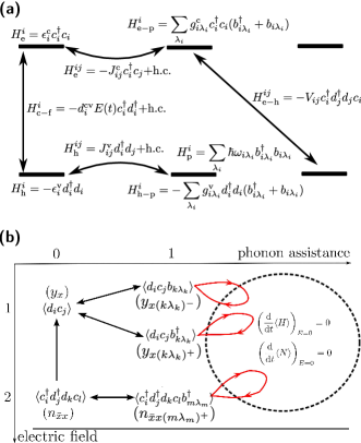
Figure 1: (Color online) (a) Illustration of the model Hamiltonian used in our study. (b) Active variables in the density matrix formalism and their interrelations in the resulting hierarchy of equations. The direction of a straight arrow indicates that in the equation for the variable at its start appears the variable at its end. Loops represent couplings to higher-order phonon-assisted density matrices which are truncated so that the particle number and energy of the free system are conserved.

The model Hamiltonian is pictorially presented in Fig. 1(a), the total Hamiltonian being

$$H=H_{\mathrm{c}}+H_{\mathrm{p}}+H_{\mathrm{c-p}}+H_{\mathrm{c-f}}.$$ (1)

Interacting carriers are described by

$$\begin{split}H_{\mathrm{c}}=\sum_{i=0}^{2N-1}\left(H^{i}_{\mathrm{e}}+H^{i}_{\mathrm{h}}+\sum_{\begin{subarray}{c}j=0\\ j\neq i\end{subarray}}^{2N-1}\left(H^{ij}_{\mathrm{e}}+H^{ij}_{\mathrm{h}}\right)+\sum_{j=0}^{2N-1}H^{ij}_{\mathrm{e}-\mathrm{h}}\right),\end{split}$$ (2)

the phonon Hamiltonian is

$$H_{\mathrm{p}}=\sum_{i=0}^{2N-1}H^{i}_{\mathrm{p}},$$ (3)

the carrier-phonon interaction is

$$H_{\mathrm{c-p}}=\sum_{i=0}^{2N-1}\left(H^{i}_{\mathrm{e}-\mathrm{p}}+H^{i}_{\mathrm{h}-\mathrm{p}}\right),$$ (4)

while the interaction of carriers with the external exciting field $E(t)$ is given as

$$H_{\mathrm{c-f}}=\sum_{i=0}^{2N-1}H^{i}_{\mathrm{c}-\mathrm{f}}.$$ (5)

In Fig. 1(a), Fermi operators $c_{i}^{\dagger}$ and $d_{i}^{\dagger}$ ($c_{i}$ and $d_{i}$) create (destroy) electrons and holes on site $i$, whereas Bose operators $b_{i\lambda_{i}}^{\dagger}$ ($b_{i\lambda_{i}}$) create (destroy) phonons in mode $\lambda_{i}$ on site $i$. $\epsilon^{\mathrm{c}}_{i}$ and $\epsilon^{\mathrm{v}}_{i}$ are electron and hole on-site energies, while $J^{\mathrm{c}}_{ij}$ and $J^{\mathrm{v}}_{ij}$ denote electron and hole transfer integrals, respectively. The carrier-phonon interaction is taken to be of the Holstein form, where a charge carrier is locally and linearly coupled to dispersionless optical modes, and $g^{\mathrm{c}}_{i\lambda_{i}}$ and $g^{\mathrm{v}}_{i\lambda_{i}}$ are the interaction strengths with electrons and holes, respectively. Electron-hole interaction is accounted for in the lowest monopole-monopole approximation and $V_{ij}$ is the carrier-carrier interaction potential. Interband dipole matrix elements are denoted by $d^{\mathrm{c}\mathrm{v}}_{i}$.

II.2 Theoretical approach to exciton dynamics

We examine the ultrafast exciton dynamics during and after pulsed photoexcitation of a heterointerface in the previously developed framework of the density matrix theory complemented with the dynamics controlled truncation (DCT) scheme Axt and Stahl (1994); Axt et al. (1996); Axt and Mukamel (1998) (see Ref. Janković and Vukmirović, 2015 and references therein), starting from initially unexcited heterojunction. We confine ourselves to the case of weak optical field and low carrier densities, in which it is justified to work in the subspace of single-exciton excitations (spanned by the so-called exciton basis) and truncate the carrier branch of the hierarchy of equations for density matrices retaining only contributions up to the second order in the optical field. The phonon branch of the hierarchy is truncated independently so as to ensure the particle-number and energy conservation after the pulsed excitation, as described in detail in Ref. Janković and Vukmirović, 2015.

In more detail, the exciton basis is obtained solving the eigenvalue problem

$$\sum_{i^{\prime}j^{\prime}}\left(\delta_{i^{\prime}i}\epsilon^{\mathrm{c}}_{jj^{\prime}}-\delta_{j^{\prime}j}\epsilon^{\mathrm{v}}_{ii^{\prime}}-\delta_{i^{\prime}i}\delta_{j^{\prime}j}V_{ij}\right)\psi^{x}_{i^{\prime}j^{\prime}}=\hbar\omega_{x}\psi^{x}_{ij},$$ (6)

where indices $i,i^{\prime}$ ($j,j^{\prime}$) correspond to the position of the hole (electron) and quantities $\epsilon^{\mathrm{c}}_{mn}$ ($\epsilon^{\mathrm{v}}_{mn}$) denote on-site electron (hole) energies (for $m=n$) or electron (hole) transfer integrals (for $m\neq n$) in the donor, in the acceptor, or between the donor and the acceptor. The creation operator for the exciton in the state $x$ is then defined as

$$X_{x}^{\dagger}=\sum_{ij}\psi^{x}_{ij}c_{j}^{\dagger}d_{i}^{\dagger}.$$ (7)

As we pointed out, Janković and Vukmirović (2015) the total Hamiltonian, in which only contributions whose expectation values are at most of the second order in the optical field are kept, can be expressed in terms of exciton operators $X_{x}^{\dagger},X_{x}$ as

$$\begin{split}H=&\sum_{x}\hbar\omega_{x}X_{x}^{\dagger}X_{x}+\sum_{i\lambda_{i}}\hbar\omega_{i\lambda_{i}}b_{i\lambda_{i}}^{\dagger}b_{i\lambda_{i}}\\ +&\sum_{\begin{subarray}{c}\bar{x}x\\ i\lambda_{i}\end{subarray}}\left(\Gamma^{i\lambda_{i}}_{\bar{x}x}X_{\bar{x}}^{\dagger}X_{x}b_{i\lambda_{i}}^{\dagger}+\Gamma^{i\lambda_{i}*}_{\bar{x}x}X_{x}^{\dagger}X_{\bar{x}}b_{i\lambda_{i}}\right)\\ -&E(t)\sum_{x}\left(M_{x}^{*}X_{x}+M_{x}X_{x}^{\dagger}\right),\end{split}$$ (8)

where the exciton-phonon coupling constants are given as

$$\Gamma^{i\lambda_{i}}_{\bar{x}x}=g^{\mathrm{c}}_{i\lambda_{i}}\sum_{j}\psi^{\bar{x}*}_{ji}\psi^{x}_{ji}-g^{\mathrm{v}}_{i\lambda_{i}}\sum_{j}\psi^{\bar{x}*}_{ij}\psi^{x}_{ij},$$ (9)

while the dipole moment for the generation of the state $x$ from the ground state is

$$M_{x}=\sum_{i}\psi^{x*}_{ii}d^{\mathrm{c}\mathrm{v}}_{i}.$$ (10)

Active variables in our formalism are the coherences between exciton state $x$ and the ground state, $y_{x}=\langle X_{x}\rangle$, exciton populations (for $\bar{x}=x$), and exciton-exciton coherences (for $\bar{x}\neq x$) $n_{\bar{x}x}=\langle X_{\bar{x}}^{\dagger}X_{x}\rangle$, together with their single-phonon-assisted counterparts $y_{x(i\lambda_{i})^{-}}=\langle X_{x}b_{i\lambda_{i}}\rangle$, $y_{x(i\lambda_{i})^{+}}=\langle X_{x}b_{i\lambda_{i}}^{\dagger}\rangle$, and $n_{\bar{x}x(i\lambda_{i})^{+}}=\langle X_{\bar{x}}^{\dagger}X_{x}b_{i\lambda_{i}}^{\dagger}\rangle$. Their mutual interrelations in the resulting hierarchy are schematically shown in Fig. 1(b), while the equations themselves are presented in Supplemental Material.  In order to quantitatively monitor ultrafast processes at the model heterojunction during and after its pulsed photoexcitation, the incoherent population of exciton state $x$, which gives the number of truly bound (Coulomb-correlated) electron-hole pairs in the state $x$,

$$\bar{n}_{xx}=n_{xx}-|y_{x}|^{2},$$ (11)

will be used. Coherent populations of exciton states, $|y_{x}|^{2}$, dominate early stages of the optical experiment, typically decay quickly due to different scattering mechanisms (in our case, the carrier-phonon interaction), and do not represent bound electron-hole pairs. The populations of truly bound electron-hole pairs build up on the expense of coherent exciton populations. We frequently normalize $\bar{n}_{xx}$ to the total exciton population in the system,

$$N_{\mathrm{tot}}=\sum_{x}n_{xx},$$ (12)

which, together with the expectation value of the Hamiltonian $\langle H\rangle$, is conserved in the absence of the external field. Probabilities $f_{\mathrm{e}}(t,r)$ [$f_{\mathrm{h}}(t,r)$] that an electron (a hole) is located at site $r$ at instant $t$ can be obtained using the so-called contraction identities (see, e.g., Ref. Axt and Mukamel, 1998) and are given as

$$f_{\mathrm{e}}(t,r)=\frac{\sum_{\bar{x}x}\left(\sum_{r_{\mathrm{h}}}\psi^{\bar{x}*}_{r_{\mathrm{h}}r}\psi^{x}_{r_{\mathrm{h}}r}\right)n_{\bar{x}x}(t)}{\sum_{x}n_{xx}(t)},$$ (13)

$$f_{\mathrm{h}}(t,r)=\frac{\sum_{\bar{x}x}\left(\sum_{r_{\mathrm{e}}}\psi^{\bar{x}*}_{rr_{\mathrm{e}}}\psi^{x}_{rr_{\mathrm{e}}}\right)n_{\bar{x}x}(t)}{\sum_{x}n_{xx}(t)}.$$ (14)

Consequently, the probability that an electron is in the acceptor at time $t$ is

$$P^{\mathrm{e}}_{A}(t)=\sum_{r=N}^{2N-1}f_{\mathrm{e}}(t,r).$$ (15)

II.3 Model parameters and Hamiltonian spectrum

The model Hamiltonian was parameterized to yield values of band gaps, bandwidths, band offsets, and exciton binding energies that are representative of typical OPV materials. The values of model parameters used in numerical computations are summarized in Table 1.

Table 1: Values of model parameters used in calculations.

Parameter	Value
$E_{g,D}$ (meV)	1500
$E_{g,A}$ (meV)	1950
$\Delta E^{\mathrm{c}}_{DA}$ (meV)	500
$|J^{\mathrm{c}}_{D}|$ (meV)	105
$|J^{\mathrm{v}}_{D}|$ (meV)	295
$|J^{\mathrm{c}}_{A}|$ (meV)	150
$|J^{\mathrm{v}}_{A}|$ (meV)	150
$|J^{\mathrm{c}}_{DA}|,|J^{\mathrm{v}}_{DA}|$ (meV)	75
$\varepsilon_{r}$	3.0
$N$	11
$a$ (nm)	1.0
$U$ (meV)	480
$\hbar\omega_{\mathrm{p,1}}$ (meV)	10
$g_{1}$ (meV)	28.5
$\hbar\omega_{\mathrm{p,2}}$ (meV)	185
$g_{2}$ (meV)	57.0
$T$ (K)	300
$t_{0}$ (fs)	50

While these values largely correspond to the PCPDTBT/PCBM interface, we note that our goal is to reach general conclusions valid for a broad class of interfaces. Consequently, later in this study, we also vary most of the model parameters and study the effects of these variations. Figures 2(a) and 2(b) illustrate the meaning of some of the model parameters.

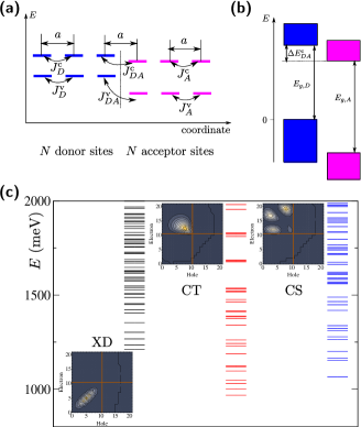
Figure 2: (Color online) (a) One-dimensional lattice model of a heterojunction. Various types of electronic couplings (in the donor, in the acceptor, and among them) are indicated. There is an energy offset between single-electron/hole levels in the donor and acceptor. (b) Band alignment produced by our model. (c) Energies of exciton states, in particular of donor excitons (black lines), CT (red lines) and CS (blue lines) states. Exciton wave function square moduli are shown for the lowest donor, CT and CS state.

All electron and hole transfer integrals are restricted to nearest neighbors. The single-particle band gap of the donor $E_{g,D}$, as well as the offset $\Delta E^{\mathrm{c}}_{DA}$ between the lowest single-electron levels in the donor and acceptor, assume values that are representative of the low-bandgap PCPDTBT polymer used in the most efficient solar cells. Hwang et al. (2007); Mühlbacher et al. (2006) The single-particle band gap of the acceptor $E_{g,A}$ and electron/hole transfer integrals $J^{\mathrm{c}/\mathrm{v}}_{A}$ are tuned to values typical of fullerene and its derivatives. Street et al. (2014); Tamura and Tsukada (2012) Electron/hole transfer integrals $J^{\mathrm{c}/\mathrm{v}}_{D}$ in the donor were extracted from the conduction and valence bandwidths of the PCPDTBT polymer. To obtain the bandwidths, an electronic structure calculation was performed on a straight infinite polymer. The calculation is based on the density functional theory (DFT) in the local density approximation (LDA), as implemented in the QUANTUM-ESPRESSO et al. (2009) package. Transfer integrals were then obtained as 1/4 of the respective bandwidth. The values of the transfer integral between the two materials are chosen to be similar to the values obtained in the ab initio study of P3HT/PCBM heterojunctions. Kanai and Grossman (2007) We set the number of sites in a single material to $N=11$, which is reasonable having in mind that the typical dimensions of phase segregated domains in bulk heterojunction morphology are considered to be $10-20$ nm. Cowan et al. (2012) The electron-hole interaction potential $V_{ij}$ is modeled using the Ohno potential

$$V_{ij}=\frac{U}{\sqrt{1+\left(\frac{r_{ij}}{a_{0}}\right)^{2}}},$$ (16)

where $r_{ij}$ is the distance between sites $i$ and $j$, and $a_{0}=e^{2}/(4\pi\varepsilon_{0}\varepsilon_{r}U)$ is the characteristic length. The relative dielectric constant $\varepsilon_{r}$ assumes a value typical for organic materials, while the magnitude of the on-site Coulomb interaction $U$ was chosen so that the exciton binding energy in both the donor and the acceptor is around 300 meV. Following common practice when studying all-organic heterojunctions, Lee et al. (2015); Bittner and Ramon (2007) we take one low-energy and one high-energy phonon mode. For simplicity, we assume that energies of both phonon modes, as well as their couplings to carriers, have the same values in both materials. The high-frequency phonon mode of energy 185 meV (approx. 1500 cm^-1), which is present in both materials, was suggested to be crucial for ultrafast electron transfer in the P3HT/PCBM blend. Falke et al. (2014) Recent theoretical calculations of the phonon spectrum and electron-phonon coupling constants in P3HT indicate the presence of low-energy phonon modes ($\lesssim 10$ meV) that strongly couple to carriers. Lücke et al. (2016) The chosen values of phonon-mode energies fall in the ranges in which the phonon density of states in conjugated polymers is large Vukmirović and Wang (2009) and the local electron-vibration couplings in PCBM are pronounced. Cheung and Troisi (2010) We estimate the carrier-phonon coupling constants from the value of polaron binding energy, which can be estimated using the result of the second-order weak-coupling perturbation theory at $T=0$ in the vicinity of the point $k=0$: Cheng and Silbey (2008)

$$\epsilon_{\mathrm{b}}^{\mathrm{pol}}=\sum_{i=1}^{2}\frac{g_{i}^{2}}{2|J|}\frac{1}{\sqrt{\left(1+\frac{\hbar\omega_{\mathrm{p},i}}{2|J|}\right)^{2}-1}}.$$ (17)

We took $g_{2}/g_{1}=2$ and estimated the numerical values assuming that $\epsilon_{\mathrm{b}}^{\mathrm{pol}}=20$ meV and $|J|=125$ meV. The electric field is centered around $t=0$ and assumes the form

$$E(t)=E_{0}\cos(\omega_{c}t)\theta(t+t_{0})\theta(t_{0}-t),$$ (18)

where $\omega_{c}$ is its central frequency, $\theta(t)$ is the step function, and the duration of the pulse is $2t_{0}$. The time $t_{0}$ should be chosen large enough so that the pulse is spectrally narrow enough (the energy of the initially generated excitons is around the central frequency of the pulse). On the other hand, since our focus is on processes happening on sub-picosecond time scale, the pulse should be as short as possible in order to disentangle the carrier generation during the pulse from free-system evolution after the pulse. Trying to reconcile the aforementioned requirements, we choose $t_{0}=50$ fs. We note that the results and conclusions to be presented do not crucially depend on the particular value of $t_{0}$ nor on the wave form of the excitation. This is shown in greater detail in Supplemental Material (Supplemental Figs. 1 and 2), where we present the dynamics for shorter pulses of wave forms given in Eqs. (18) and (33). Interband dipole matrix elements $d_{i}^{\mathrm{cv}}$ are zero in the acceptor ($i=N,\dots,2N-1$), while in the donor they all assume the same value $d^{\mathrm{cv}}$ so that $d^{\mathrm{cv}}E_{0}=0.2$ meV (weak excitation).

Figure 2(c) displays part of the exciton spectrum produced by our model. Exciton states can be classified according to the relative position of the electron and the hole. The classification is straightforward only for the noninteracting heterojunction ($J^{\mathrm{c}/\mathrm{v}}_{DA}=0$), in which case any exciton state can be classified into four groups:

• both the electron and the hole are in the donor [donor exciton (XD) state],

• both the electron and the hole are in the acceptor (acceptor exciton state),

• the electron is in the acceptor, while the hole is in the donor (space-separated exciton state),

• the electron is in the donor, while the hole is in the acceptor.

Space-separated excitons can be further discriminated according to their mean electron-hole distance defined as

$$\langle r_{\mathrm{e-h}}\rangle_{x}=\sum_{ij}|i-j||\psi^{x}_{ij}|^{2}.$$ (19)

When the electron-hole interaction is set to zero, the mean electron-hole distance for all the states from group (c) is equal to $N$. For the non-zero Coulomb interaction, we consider a space-separated exciton as a CS exciton if its mean electron-hole distance is larger than (or equal to) $N$, otherwise we consider it as a CT exciton. In the general case, the character of an exciton state is established by calculating its overlap with each of the aforementioned groups of the exciton states at the noninteracting heterojunction; this state then inherits the character of the group with which the overlap is maximal.

III Numerical results

Here, the results of our numerical calculations on the model system defined in Sec. II are presented. In Sec. III.1, we observe that the populations of CT and CS states predominantly build up during the action of the excitation, and that the changes in these populations occurring on $\sim$100-fs time scales after the excitation are rather small. This conclusion, i.e., the direct optical generation as the principal source of space-separated charges on ultrafast time scales following the excitation, is shown in Sec. III.2 to be robust against variations of model parameters. Since the focus of our study is on the ultrafast exciton dynamics at photoexcited heterojunctions, all the computations are carried out for 1 ps in total (involving the duration of the pulse).

III.1 Interfacial dynamics on ultrafast time scales

Figure 3(a) shows the time dependence of the numbers of donor, CT, and CS excitons for the 100-fs-long excitation with central frequency $\hbar\omega_{c}=1500$ meV, which excites the system well above the lowest donor or space-separated exciton state, see Fig. 2(c).

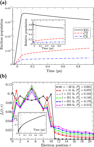
Figure 3: (Color online) (a) Time dependence of the numbers of donor (XD), CT, and CS excitons. The inset shows the time dependence of these quantities normalized to the total exciton population in the system. (b) Probability that at time $t$ an electron is located at site $r$ as a function of $r$ for various values of $t$. In the legend, the probability that at instant $t$ an electron is located in the acceptor is given, while the inset shows its full time dependence. Dotted vertical lines indicate the end of the excitation.

The number of all three types of excitons grows during the action of the electric field, whereas after the electric field has vanished, the number of donor excitons decreases and the numbers of CT and CS excitons increase. However, the changes in the exciton numbers brought about by the free-system evolution alone are much less pronounced than the corresponding changes during the action of the electric field, as is shown in Fig. 3(a). The population of CS excitons builds up during the action of the electric field, so that after the first 100 fs of the calculation, CS excitons comprise 7.6% of the total exciton population, see the inset of Fig. 3(a). In the remaining 900 fs, when the dynamics is governed by the free Hamiltonian, the population of CS excitons further increases to 9.6%. A similar, but less extreme, situation is also observed in the relative number of CT excitons, which at the end of the pulse form 14% of the total population and in the remaining 900 fs of the computation their number further grows to 24%. Therefore, if only the free-system evolution were responsible for the conversion from donor to CT and CS excitons, the population of CT and CS states at the end of the pulsed excitation would assume much smaller values than we observe. We are led to conclude that the population of CT and CS excitons on ultrafast ($\lesssim 100$-fs) time scales is mainly established by direct optical generation. Transitions from donor to CT and CS excitons are present, but on this time scale are not as important as is currently thought.

Exciton dissociation and charge separation can also be monitored using the probabilities $f_{\mathrm{e}}(t,r)$ [$f_{\mathrm{h}}(t,r)$] that an electron (a hole) is located on site $r$ at instant $t$, as well as the probability $P^{\mathrm{e}}_{A}(t)$ that an electron is in the acceptor at time $t$, see Eqs. (13)–(15). Figure 3(b) displays quantity $f_{\mathrm{e}}$ as a function of site index $r$ at different times $t$. The probability of an electron being in the acceptor is a monotonically increasing function of time $t$, see the inset of Fig. 3(b). It increases, however, more rapidly during the action of the electric field than after the electric field has vanished: in the first 100 fs of the calculation, it increases from virtually 0 to 0.070, while in the next 100 fs it only rises from 0.070 to 0.104, and at the end of the computation it assumes the value 0.210. The observed time dependence of the probability that an electron is located in the acceptor further corroborates our hypothesis of direct optical generation as the main source of separated carriers on ultrafast time scales. If only transitions from donor to CT and CS excitons led to ultrafast charge separation starting from a donor exciton, the values of the considered probability would be smaller than we observe.

The rationale behind the direct optical generation of space-separated charges is the resonant coupling between donor excitons and (higher-lying) space-separated states, which stems from the resonant mixing between single-electron states in the donor and acceptor modulated by the electronic coupling between materials, see the level alignment in Fig. 2(b). This mixing leads to higher-lying CT and CS states having non-negligible amount of donor character and acquiring nonzero dipole moment from donor excitons; these states can thus be directly generated from the ground state. It should be stressed that the mixing, in turn, influences donor states, which have certain amount of space-separated character.

III.2 Impact of model parameters on ultrafast exciton dynamics

Our central conclusion was so far obtained using only one set of model parameters and it is therefore important to check its sensitivity on system parameters. To this end, we vary one model parameter at a time, while all the other parameters retain the values listed in Table 1.

We start by investigating the effect of the transfer integral between the donor and acceptor $J^{\mathrm{c}/\mathrm{v}}_{DA}$. Higher values of $J^{\mathrm{c}/\mathrm{v}}_{DA}$ favor charge separation, since the relative numbers of CT and CS excitons, together with the probability that an electron is in the acceptor, increase, whereas the relative number of donor excitons decreases with increasing $J^{\mathrm{c}/\mathrm{v}}_{DA}$, see Figs. 4(a)–4(c).

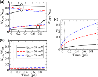
Figure 4: (Color online) Time dependence of the relative number of (a) donor and CT, (b) CS excitons, and (c) the probability $P^{\mathrm{e}}_{A}$ that an electron is in the acceptor, for different values of the transfer integrals $|J^{\mathrm{c}}_{DA}|=|J^{\mathrm{v}}_{DA}|=J_{DA}$ between the donor and the acceptor. Dotted vertical lines indicate the end of the excitation.

In light of the proposed mechanism of ultrafast direct optical generation of space-separated charges, the observed trends can be easily rationalized. Stronger electronic coupling between materials leads to stronger mixing between donor and space-separated states, i.e., a more pronounced donor character of CT and CS states and consequently a larger dipole moment for direct creation of CT and CS states from the ground state.

The results concerning the effects of the energy offset $\Delta E^{\mathrm{c}}_{DA}$ between LUMO levels in the donor and acceptor are summarized in Figs. 5(a)–5(c).

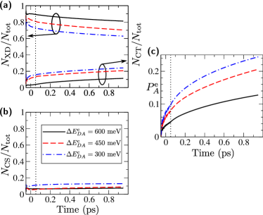
Figure 5: (Color online) Time dependence of the relative number of (a) donor and CT, (b) CS excitons, and (c) the probability $P^{\mathrm{e}}_{A}$ that an electron is in the acceptor, for different values of the LUMO-LUMO energy offset $\Delta E^{\mathrm{c}}_{DA}$. Dotted vertical lines indicate the end of the excitation.

The parameter $\Delta E^{\mathrm{c}}_{DA}$ determines the energy width of the overlap region between single-electron states in the donor and acceptor, see Fig. 2(b). The smaller is $\Delta E^{\mathrm{c}}_{DA}$, the greater is the number of virtually resonant single-electron states in the donor and in the acceptor and therefore the greater is the number of (higher-lying) CT and CS states that inherit nonzero dipole moments from donor states and may thus be directly excited from the ground state. This manifests as a larger number of CT and CS excitons, as well as a larger probability that an electron is in the acceptor, with decreasing $\Delta E^{\mathrm{c}}_{DA}$.

Figures 6(a)–6(c) show the effects of electron delocalization in the acceptor on the ultrafast dynamics at the model heterojunction.

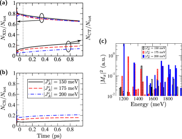
Figure 6: (Color online) Time dependence of the relative number of (a) donor and CT, and (b) CS excitons, for different values of electronic coupling in the acceptor $J^{\mathrm{c}}_{A}$. (c) Squared moduli of dipole matrix elements (in arbitrary units) for direct generation of CS excitons from the ground state for different values of electronic coupling in the acceptor $J^{\mathrm{c}}_{A}$. Dotted vertical lines indicate the end of the excitation. Note that, globally, squared moduli of dipole matrix elements are largest for $|J^{\mathrm{c}}_{A}|=200$ meV (completely filled bars).

Delocalization effects are mimicked by varying the electronic coupling in the acceptor. While increasing $|J^{\mathrm{c}}_{A}|$ has virtually no effect on the relative number of donor excitons, it leads to an increased participation of CS and a decreased participation of CT excitons in the total exciton population. CT states, in which the electron-hole interaction is rather strong, are mainly formed from lower-energy single-electron states in the acceptor and higher-energy single-hole states in the donor. These single-particle states are not subject to strong resonant mixing with single-particle states of the other material. However, CS states are predominantly composed of lower-energy single-hole donor states and higher-energy single-electron acceptor states; the mixing of the latter group of states with single-electron donor states is stronger for larger $|J^{\mathrm{c}}_{A}|$, just as in case of smaller $\Delta E^{\mathrm{c}}_{DA}$, see Fig. 2(b). Therefore the dipole moments for direct generation of CS excitons generally increase when increasing $|J^{\mathrm{c}}_{A}|$, see Fig. 6(c), whereas the dipole moments for direct generation of CT excitons at the same time change only slightly, which can account for the trends of the participation of CS and CT excitons in Figs. 6(a) and 6(b).

We now turn our attention to the effects that the strength of the carrier-phonon interaction has on the ultrafast exciton dynamics at heterointerfaces.

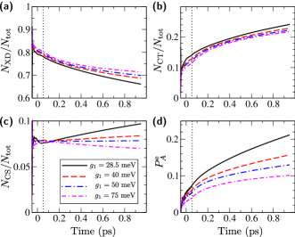
Figure 7: (Color online) Time dependence of the relative number of (a) donor, (b) CT , (c) CS excitons, and (d) the probability $P^{\mathrm{e}}_{A}$ that an electron is in the acceptor, for different strengths of the carrier-phonon interaction. Dotted vertical lines indicate the end of the excitation.

In Figs. 7(a)–7(d), we present the results with the fixed ratio $g_{2}/g_{1}=2.0$ and the polaron binding energies defined in Eq. (17) assuming the values of approximately 20, 40, 60, and 140 meV, in ascending order of $g_{1}$. We note that it is not straightforward to predict the effect of the variations of carrier-phonon interaction strength on the population of space-separated states. Single-phonon-assisted processes preferentially couple exciton states of the same character, i.e., a donor exciton state is more strongly coupled to another donor state, than to a space-separated state. On the one hand, stronger carrier-phonon interaction implies more pronounced exciton dissociation and charge separation because of stronger coupling between donor and space-separated states. On the other hand, stronger carrier-phonon interaction leads to faster relaxation of initially generated donor excitons within the donor exciton manifold to low-lying donor states. Low-lying donor states are essentially uncoupled from space-separated states, i.e., they exhibit low probabilities of exciton dissociation and charge separation. Our results, shown in Figs. 7(a)–7(d), indicate that stronger carrier-phonon interaction leads to smaller number of CT and CS excitons, as well as the probability that an electron is in the acceptor, and to greater number of donor excitons. We also note that stronger carrier-phonon interaction changes the trend displayed by the population of CS states. While for the weakest interaction studied CS population grows after the excitation, for the strongest interaction studied CS population decays after the excitation. This is a consequence of more pronounced phonon-assisted processes leading to population of low-energy CT states once a donor exciton performs a transition to a space-separated state. This discussion can rationalize the changes in relevant quantities summarized in Figs. 7(a)- 7(d); the magnitudes of the changes observed are, however, rather small. In previous studies, Lee et al. (2015); Bera et al. (2015) which did not deal with the initial exciton generation step, stronger carrier-phonon interaction is found to suppress quite strongly the charge separation process. The weak influence of the carrier-phonon interaction strength on ultrafast heterojunction dynamics that we observe supports the mechanism of ultrafast direct optical generation of space-separated charges. If the charge separation process at heterointerfaces were mainly driven by the free-system evolution, greater changes in the quantities describing charge separation efficiency would be expected with varying carrier-phonon interaction strength.

Additionally, we have performed computations for a fixed value of $\epsilon^{\mathrm{pol}}_{\mathrm{b}}$ [Eq. (17)] and different values of the ratio $g_{2}/g_{1}$ among coupling constants of high- and low-frequency phonon modes. The result, which is presented in Supplemental Material (Supplemental Fig. 4), shows that the increase of the ratio $g_{2}/g_{1}$ increases the number of CT excitons and decreases the number of donor excitons, while the population of CS states exhibits only a weak increase. Stronger coupling to the high-frequency phonon mode (with respect to the low-frequency one) enhances charge separation by decreasing the number of donor excitons, but at the same time promotes phonon-assisted processes towards more strongly bound CT states, so that the population of CS states remains nearly constant.

Our formalism takes into account the influence of phonons on excitons. However, if this influence were too strong, the hierarchy of equations would have to be truncated at a higher level, which would make it computationally intractable. When the effects of lattice motion on excitons are strong, one has, in turn, to consider the feedback of excitons on phonons, which is not captured by the current approach. The feedback of excitons on the lattice motion can be easily included in a mixed quantum/classical approach, where excitons are treated quantum mechanically, while the lattice motion is treated classically. To estimate the importance of the feedback of excitons on the lattice motion, we have performed the computation using the surface hopping approach Tully (1990); Wang and Prezhdo (2014) (see Supplemental Material for more details). In Supplemental Fig. 3 we show the time dependence of the probability that an electron is in the acceptor obtained from simulations with and without feedback effects. The result is nearly the same in both cases, suggesting that feedback effects are small. As a consequence, our approach is sufficient for properly taking into account the influence of phonons on excitons.

We have also studied the influence of the temperature on the ultrafast exciton dynamics at a heterojunction. It exhibits a weak temperature dependence, see Supplemental Fig. 5, which is consistent with existing theoretical Chenel et al. (2014) and experimental Pensack and Asbury (2010) insights, and also with the mechanism of direct optical generation of space-separated carriers.

Finally, the consequences of introducing diagonal static disorder in our model will be studied. It is done by drawing the (uncorrelated) on-site energies of electrons and holes in the donor and the acceptor from Gaussian distributions centered at the values that can be obtained from Table 1. We have for simplicity assumed that the standard deviations of all the Gaussian distributions are equal to $\sigma$. As we do not intend to obtain any of the system properties by a statistical analysis of various realizations of disorder, but merely to check whether or not the presence of disorder may significantly alter qualitative features of the proposed picture of ultrafast exciton dynamics at heterointerfaces, we present our results only for a couple of different disorder realizations and compare them to the results for ordered system. In Figs. 8(a)–8(d) we show the time dependence of the relative number of space-separated (CS and CT) excitons and of the probability $P^{\mathrm{e}}_{A}$ for three different realizations of disorder with standard deviations $\sigma=50$ and $100$ meV.

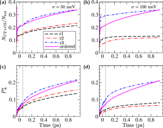
Figure 8: (Color online) (a) and (b) Time dependence of the relative number of space-separated (CT and CS) excitons for three different disorder realizations (r1,r2,and r3). (c) and (d) Time dependence of the probability that an electron is in the acceptor for three different disorder realizations. Time evolution of the respective quantities in ordered system is shown on each graph for comparison. Disorder is diagonal (affects only on-site energies), static, and Gaussian, standard deviations being $\sigma=50$ [(a) and (c)] and $100$ meV [(b) and (d)].

For these disorder realizations, the quantities we use to describe ultrafast heterojunction dynamics show qualitatively similar behavior to the case of the ordered system. Namely, changes in the relative number of space-separated excitons and the probability of an electron being in the acceptor are more pronounced during the action of the pulse than after its end. The characteristic time scales of these changes (for the disorder realizations studied) are not drastically different from the corresponding time scale in the ordered system. The presence of disorder in our model does not necessarily lead to less efficient charge separation as monitored by the two aforementioned quantities. Our results based on the considered disorder realizations are in agreement with the more detailed study of the effects of disorder on charge separation at model D/A interfaces, Vázquez and Troisi (2013) from which emerged that regardless of the degree of disorder, the essential physics of free hole and electron generation remains the same.

In summary, we find that regardless of the particular values of varied model parameters ($J^{\mathrm{c}/\mathrm{v}}_{DA},\Delta E^{\mathrm{c}}_{DA},J^{\mathrm{c}}_{A}$, carrier-phonon coupling constants), the majority of CT and CS states that are present at $\sim 100$ fs after photoexcitation have been directly generated during the excitation. Trends in quantities describing ultrafast heterojunction dynamics that we observe varying model parameters can be explained by taking into consideration the proposed mechanism of ultrafast direct optical generation of space-separated charges.

IV Ultrafast spectroscopy signatures

Exciton dynamics on ultrafast time scales is typically probed experimentally using the ultrafast pump-probe spectroscopy, see, e.g., Refs. Grancini et al., 2013; Jailaubekov et al., 2013. In such experiments, the presence of space-separated charges on ultrafast time scales after photoexcitation has been established and the energy resonance between donor exciton and space-separated states was identified as responsible for efficient charge generation, Grancini et al. (2013) in agreement with our numerical results. However, while our results indicate that the majority of space-separated charges that are present at $\sim 100$ fs after photoexcitation have been directly optically generated, interpretation of experiments Grancini et al. (2013) suggests that these states become populated by the transition from donor exciton states. To understand the origin of this apparent difference, we numerically compute ultrafast pump-probe signals in the framework of our heterojunction model. In Sec. IV.1, we present the theoretical treatment of ultrafast pump-probe experiments adapted for the system at hand. Assuming that the probe pulse is deltalike, we obtain an analytic expression relating the differential transmission $\Delta T$ to the nonequilibrium state of the system “seen” by the probe pulse. The expression provides a very clear and direct interpretation of the results of ultrafast pump-probe experiments and allows to distinguish between contributions stemming from exciton populations and coherences, challenging the existing interpretations. It is used in Sec. IV.2 to numerically compute differential transmission signals.

IV.1 Theoretical treatment of the ultrafast pump-probe spectroscopy

In a pump-probe experiment, the sample is firstly irradiated by an energetic pump pulse and the resulting excited (nonequilibrium) state of the sample is consequently examined using a second, weaker, probe pulse, whose time delay with respect to the pump pulse can be tuned. Mukamel (1995); Cabanillas-Gonzalez et al. (2011); Perfetto and Stefanucci (2015) Our theoretical approach to a pump-probe experiment considers the interaction with the pump pulse as desribed in Sec. II.2 and Ref. Janković and Vukmirović, 2015, i.e., within the density matrix formalism employing the DCT scheme up to the second order in the pump field. The interaction with the probe pulse is assumed not to change significantly the nonequilibrium state created by the pump pulse and is treated in the linear response regime. The corresponding nonequilibrium dipole-dipole retarded correlation function is then used to calculate pump-probe signals. Perfetto and Stefanucci (2015); Walkenhorst et al. (2016)

To study pump-probe experiments, we extended our two-band lattice semiconductor model including more single-electron (single-hole) energy levels per site. Multiple single-electron (single-hole) levels on each site should be dipole-coupled among themselves in order to enable probe-induced dipole transitions between various exciton states. We denote by $c_{i\beta_{i}}^{\dagger}$ ($c_{i\beta_{i}}$) creation (annihilation) operators for electrons on site $i$ in conduction-band orbital $\beta_{i}$; similarly, $d_{i\alpha_{i}}^{\dagger}$ ($d_{i\alpha_{i}}$) create (annihilate) a hole on site $i$ in valence-band orbital $\alpha_{i}$. The dipole-moment operator in terms of electron and hole operators assumes the form

$$\begin{split}P&=\sum_{\begin{subarray}{c}i\\ \beta_{i}\alpha_{i}\end{subarray}}\left(d^{\mathrm{cv}}_{i}c_{i\beta_{i}}^{\dagger}d_{i\alpha_{i}}^{\dagger}+\mathrm{h.c.}\right)\\ &+\sum_{\begin{subarray}{c}i\\ \beta_{i}\neq\beta_{i}^{\prime}\end{subarray}}d^{\mathrm{cc}}_{i}c_{i\beta_{i}}^{\dagger}c_{i\beta_{i}^{\prime}}-\sum_{\begin{subarray}{c}i\\ \alpha_{i}\neq\alpha_{i}^{\prime}\end{subarray}}d^{\mathrm{vv}}_{i}d_{i\alpha_{i}^{\prime}}^{\dagger}d_{i\alpha_{i}}.\end{split}$$ (20)

Intraband dipole matrix elements $d^{\mathrm{cc}}_{i}$ ($d^{\mathrm{vv}}_{i}$) describe electron (hole) transitions between different single-electron (single-hole) states on site $i$, as opposed to the interband matrix elements $d^{\mathrm{c}\mathrm{v}}_{i}$, which are responsible for the exciton generation. Performing transition to the exciton basis, which is defined analogously to Eq. (6), dipole matrix elements for transitions from the ground state to exciton state $x$ are

$$M_{x}=\sum_{\begin{subarray}{c}i\\ \beta_{i}\alpha_{i}\end{subarray}}d^{\mathrm{cv}}_{i}\psi_{(i\alpha_{i})(i\beta_{i})}^{x*},$$ (21)

while those for transitions from exciton state $x$ to exciton state $\bar{x}$ are

$$\begin{split}M_{\bar{x}}^{x}&=\sum_{\begin{subarray}{c}i\\ \alpha_{i}\neq\alpha_{i}^{\prime}\end{subarray}}\sum_{\begin{subarray}{c}j\\ \beta_{j}\end{subarray}}\psi_{(i\alpha_{i})(j\beta_{j})}^{\bar{x}*}d^{\mathrm{vv}}_{i}\psi_{(i\alpha_{i}^{\prime})(j\beta_{j})}^{x}\\ &-\sum_{\begin{subarray}{c}i\\ \beta_{i}\neq\beta_{i}^{\prime}\end{subarray}}\sum_{\begin{subarray}{c}j\\ \alpha_{j}\end{subarray}}\psi_{(j\alpha_{j})(i\beta_{i}^{\prime})}^{\bar{x}*}d^{\mathrm{cc}}_{i}\psi_{(j\alpha_{j})(i\beta_{i})}^{x}.\end{split}$$ (22)

Operator $P$ [Eq. (20)] expressed in terms of operators $X_{x},X_{x}^{\dagger}$ assumes the form (keeping only contributions whose expectation values are at most of the second order in the pump field)

$$P=\sum_{x}\left(M_{x}X_{x}^{\dagger}+M_{x}^{*}X_{x}\right)-\sum_{\bar{x}x}M_{\bar{x}}^{x}X_{\bar{x}}^{\dagger}X_{x}.$$ (23)

We concentrate on the so-called nonoverlapping regime, Perfetto and Stefanucci (2015) in which the probe pulse, described by its electric field $e(t)$, acts after the pump pulse. We take that our system meets the condition of optical thinness, i.e., the electromagnetic field originating from probe-induced dipole moment can be neglected compared to the electromagnetic field of the probe. In the following considerations, the origin of time axis $t=0$ is taken to be the instant at which the probe pulse starts. The pump pulse finishes at $t=-\tau$, where $\tau$ is the time delay between (the end of) the pump and (the start of) the probe. The pump creates a nonequilibrium state of the system which is, at the moment when the probe pulse starts, given by the density matrix $\rho(0)$, which implicitly depends on the pump-probe delay $\tau$.

In the linear-response regime, the probe-induced dipole moment $d_{p}(t)$ for $t>0$ is expressed as Perfetto and Stefanucci (2015)

$$d_{p}(t)=\int\mathrm{d}t^{\prime}\mbox{\hskip 1.70717pt}\chi(t,t^{\prime})\mbox{\hskip 1.70717pt}e(t^{\prime}),$$ (24)

where $\chi(t,t^{\prime})$ is the nonequilibrium retarded dipole-dipole correlation function

$$\chi(t,t^{\prime})=-\frac{\mathrm{i}}{\hbar}\theta(t-t^{\prime})\mbox{\hskip 1.70717pt}\mathrm{Tr}\left(\rho(0)[P(t),P(t^{\prime})]\right).$$ (25)

Time dependence in Eq. (25) is governed by the Hamiltonian of the system in the absence of external fields [Eq. (8)]

$$H_{E(t)=0}=H_{0}+H_{\mathrm{e-ph}},$$ (26)

where $H_{0}$ is the noninteracting Hamiltonian of excitons in the phonon field [the first two terms in Eq. (8)], while $H_{\mathrm{e-ph}}$ accounts for exciton-phonon interaction [the third term in Eq. (8)]. For an ultrashort probe pulse, $e(t)=e_{0}\delta(t)$, the probe-induced dipole moment assumes the form

$$d_{p}(t)=e_{0}\chi(t,0)=e_{0}\left(-\frac{\mathrm{i}}{\hbar}\right)\mathrm{Tr}\left(\rho(0)[P(t),P(0)]\right).$$ (27)

Probe pulse tests the possibility of transitions between various exciton states, i.e., it primarily affects carriers. Therefore, as a reasonable approximation to the full time dependent operator $P(t)$ appearing in Eq. (27), operator $P^{(0)}(t)$, evolving according to the noninteracting Hamiltonian $H_{0}$ in Eq. (26), may be used. This leads us to the central result for the probe-induced dipole moment:

$$d_{p}(t)=e_{0}\left(-\frac{\mathrm{i}}{\hbar}\right)\mathrm{Tr}\left(\rho(0)[P^{(0)}(t),P(0)]\right).$$ (28)

Deriving the commutator in Eq. (28), in the expression for $d_{p}(t)$ we obtain two types of contributions, see Eq. (38) in Appendix A. Contributions of the first type oscillate at frequencies $\omega_{x}$ corresponding to probe-induced transitions between the ground state and exciton state $x$, while those of the second type oscillate at frequencies $\omega_{\bar{x}}-\omega_{x}$ corresponding to probe-induced transitions between exciton states $\bar{x}$ and $x$. Here, we focus our attention to the process of photoinduced absorption (PIA), in which an exciton in state $x$ performs a transition to another state $\bar{x}$ under the influence of the probe field. Therefore we will further consider only the second type of contributions.

The frequency-dependent transmission coefficient $T(\omega)$ is defined as (we use SI units)

$$T(\omega)=1+\frac{c\mu_{0}}{\mathcal{S}\hbar}\mbox{\hskip 1.70717pt}\mathrm{Im}\left\{\hbar\omega\mbox{\hskip 1.70717pt}\frac{d_{p}(\omega)}{e(\omega)}\right\},$$ (29)

where $d_{p}(\omega)$ and $e(\omega)$ are Fourier transformations of $d_{p}(t)$ and $e(t)$, respectively, while $\mathcal{S}$ is the irradiated area of the sample. The differential transmission is given as

$$\Delta T(\tau;\omega)=T^{\mathrm{neq}}(\tau;\omega)-T^{\mathrm{eq}}(\omega).$$ (30)

The transmission of a system, which is initially (before the action of the probe) unexcited, is denoted by $T^{\mathrm{eq}}(\omega)$. The transmission of a pump-driven system $T^{\mathrm{neq}}(\tau;\omega)$ depends on the time delay $\tau$ between the pump and the probe through the nonequilibrium density matrix $\rho(0)$. Since our aim is to study the process of PIA and since $T^{\mathrm{eq}}(\omega)$ is expected to reflect only transitions involving the ground state, we will not further consider this term. After a derivation, the details of which are given in Appendix A, we obtain the expression for the part of the differential transmission signal $\Delta T_{\mathrm{PIA}}(\tau;\omega)$ accounting for the PIA:

$$\begin{split}\Delta T_{\mathrm{PIA}}(\tau;\omega)&\propto\mathrm{Im}\left\{\sum_{xx^{\prime}}\left((M_{x}M^{x}_{x^{\prime}})^{*}\frac{\hbar\omega}{\hbar\omega-(\hbar\omega_{x^{\prime}}-\hbar\omega_{x})+\mathrm{i}\eta}y_{x^{\prime}}(0)-M_{x}M^{x}_{x^{\prime}}\frac{\hbar\omega}{\hbar\omega+(\hbar\omega_{x^{\prime}}-\hbar\omega_{x})+\mathrm{i}\eta}y_{x^{\prime}}^{*}(0)\right)\right.+\\ &+\left.\sum_{\bar{x}xx^{\prime}}\left(M^{x}_{x^{\prime}}M^{\bar{x}}_{x}\frac{\hbar\omega}{\hbar\omega+(\hbar\omega_{x^{\prime}}-\hbar\omega_{x})+\mathrm{i}\eta}y_{x^{\prime}}^{*}(0)y_{\bar{x}}(0)-M^{x^{\prime}}_{x}M^{x}_{\bar{x}}\frac{\hbar\omega}{\hbar\omega-(\hbar\omega_{x^{\prime}}-\hbar\omega_{x})+\mathrm{i}\eta}y_{\bar{x}}^{*}(0)y_{x^{\prime}}(0)\right)\right.+\\ &+\left.\sum_{\bar{x}xx^{\prime}}\left(M^{x}_{x^{\prime}}M^{\bar{x}}_{x}\frac{\hbar\omega}{\hbar\omega+(\hbar\omega_{x^{\prime}}-\hbar\omega_{x})+\mathrm{i}\eta}\bar{n}_{x^{\prime}\bar{x}}(0)-M^{x^{\prime}}_{x}M^{x}_{\bar{x}}\frac{\hbar\omega}{\hbar\omega-(\hbar\omega_{x^{\prime}}-\hbar\omega_{x})+\mathrm{i}\eta}\bar{n}_{\bar{x}x^{\prime}}(0)\right)\right\}.\end{split}$$ (31)

In the last equation, we have explicitly separated the coherent contributions by introducing the correlated parts of exciton populations and exciton-exciton coherences $\bar{n}_{\bar{x}x}=n_{\bar{x}x}-y_{\bar{x}}^{*}y_{x}$ [see also Eq. (11) defining incoherent exciton populations], while $\eta$ is a positive parameter effectively accounting for the spectral line broadening. Walkenhorst et al. (2016) $y_{x}(0)$ denotes the value of the electronic density matrix $y_{x}$ at the moment when the probe pulse starts, and similarly for $\bar{n}_{\bar{x}x}(0)$. The coherences between exciton states and the ground state $y_{x}(0)$, as well as correlated parts of exciton-exciton coherences $\bar{n}_{\bar{x}x}(0)$ ($\bar{x}\neq x$), are expected to approach zero for sufficiently long time delays between the pump and the probe.  In this limit, Eq. (31) contains only the incoherent exciton populations $\bar{n}_{xx}$:

$$\Delta T_{\mathrm{PIA}}(\tau;\omega)\propto\sum_{xx^{\prime}}|M^{x}_{x^{\prime}}|^{2}\left(-\frac{\eta\cdot\hbar\omega}{(\hbar\omega+(\hbar\omega_{x^{\prime}}-\hbar\omega_{x}))^{2}+\eta^{2}}+\frac{\eta\cdot\hbar\omega}{(\hbar\omega-(\hbar\omega_{x^{\prime}}-\hbar\omega_{x}))^{2}+\eta^{2}}\right)\bar{n}_{x^{\prime}x^{\prime}}(0).$$ (32)

This expression is manifestly negative when it describes probe-induced transitions from exciton state $x^{\prime}$ to some higher-energy exciton state $x$. The last conclusion is in agreement with the usual experimental interpretation of pump-probe spectra, where a negative differential transmission signal corresponds either to PIA or to stimulated emission. Cabanillas-Gonzalez et al. (2011) Our expression [Eq. (31)] demonstrates, however, that this correspondence can not be uniquely established in the ultrafast regime, where it is expected that both coherences between exciton states and the ground state $y_{x}(0)$ and exciton-exciton coherences $\bar{n}_{\bar{x}x}(0)$ ($\bar{x}\neq x$), along with incoherent exciton populations $\bar{n}_{xx}(0)$, play significant role. This is indeed the case in our numerical computations of pump-probe spectra, which are presented in the following subsection. For each studied case, we separately show the total signal [full Eq. (31)], the $y$-part of the signal [the first two terms in Eq. (31)], and the $\bar{n}$-part of the signal [the third term in Eq. (31)]. We note that it would be possible to further separate the $\bar{n}$-part of the signal into the contribution stemming from incoherent exciton populations $\bar{n}_{xx}$ [Eq. (32)] and exciton-exciton coherences $\bar{n}_{\bar{x}x}$ $(\bar{x}\neq x)$. As shown in more detail in Supplemental Material (Supplemental Fig. 7), the overall $\bar{n}$-part of the signal is qualitatively very similar to its contribution stemming from incoherent exciton populations. Therefore, for the simplicity of further discussion, we may consider the $\bar{n}$-part of the signal as completely originating from incoherent exciton populations.

IV.2 Numerical results: ultrafast pump-probe signals

In order to compute pump-probe signals and at the same time keep the numerics manageable, we extended our model by introducing only one additional single-electron level both in the donor and in the acceptor and one additional single-hole level in the donor. Additional energy levels in the donor and the corresponding bandwidths are extracted from the aforementioned electronic structure calculation on the infinitely long PCPDTBT polymer. The additional single-electron level is located at 1160 meV above the single-electron level used in all the calculations and the bandwidth of the corresponding zone is estimated to be 480 meV. The additional single-hole level is located at 1130 meV below the single-hole level used in all the calculations and the bandwidth of the corresponding zone is estimated to be 570 meV. The additional single-electron level in the acceptor is extracted from an electronic structure calculation on the C₆₀ molecule. The calculation is based on DFT using either LDA or B3LYP exchange-correlation functional (both choices give similar results) and 6-31G basis set and was performed using the NWChem package. Valiev et al. (2010) We found that the additional single-electron level lies around 1000 meV above the single-electron level used in all the calculations. The bandwidth of the corresponding zone is set to 600 meV, see Table 1.

In this subsection we assume that the waveform of the pump pulse is

$$E(t)=E_{0}\cos(\omega_{c}t)\exp\left(-\frac{t^{2}}{\tau_{G}^{2}}\right)\theta(t+t_{0})\theta(t_{0}-t),$$ (33)

where we take $\tau_{G}=20$ fs and $t_{0}=50$ fs, while the probe is

$$e(t)=e_{0}\delta(t-(t_{0}+\tau)),$$ (34)

with variable pump-probe delay $\tau$. The intraband dipole matrix elements $d^{\mathrm{c}\mathrm{c}}_{i},d^{\mathrm{v}\mathrm{v}}_{i}$ in Eq. (20) are assumed to be equal in the whole system

$$d^{\mathrm{cc}}_{i}=d^{\mathrm{vv}}_{i}=d^{\mathrm{intra}}=\frac{1}{2}d^{\mathrm{c}\mathrm{v}}.$$ (35)

The positive parameter $\eta$, which effectively accounts for the line broadening, is set to $\eta=50$ meV. We have checked that variations in $\eta$ do not change the qualitative features of the presented PIA spectra, see Supplemental Fig. 6. In actual computations of the signal given in Eq. (31), we should remember that the pump pulse finishes at instant $t_{0}$, while in Eq. (31) all the quantities are taken at the moment when the probe starts, which is now $t_{0}+\tau$; in other words, $y_{x}(0)\to y_{x}(t_{0}+\tau)$, $\bar{n}_{\bar{x}x}(0)\to\bar{n}_{\bar{x}x}(t_{0}+\tau)$ when we compute pump-probe signals using Eq. (31) and the pump and probe are given by Eqs. (33) and (34), respectively.

In Figs. 9(a) and 9(b) we show the PIA signal from space-separated states after the excitation by the pump at 1500 meV. The frequency $\omega$ in Eq. (31) is set to 1000 meV, which is (for the adopted values of model parameters) appropriate for observing PIA from space-separated states. At small pump-probe delays ($\tau\lesssim 300$ fs), we see that the oscillatory features stemming from coherences between exciton states and the ground state ($y$-part of the signal) dominate the dynamics. At larger delays, the part originating from established (incoherent) exciton populations ($\bar{n}$-part of the signal) prevails, see Fig. 9(b), and the shape of the signal resembles the shapes of signals from space-separated states in Fig. 4(c) of Ref. Grancini et al., 2013. The signal decreases at larger delays, which correlates very well with the fact that the numbers of CT and CS excitons increase, see Fig. 3(a). In other words, at larger pump-probe delays, at which the influence of coherences between exciton states and the ground state is small, the signal can be unambiguously interpreted in terms of charge transfer from the donor to the acceptor.

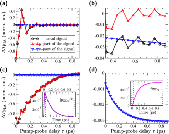
Figure 9: (Color online) Differential transmission signal $\Delta T_{\mathrm{PIA}}$ [Eq. (31)] as a function of the pump-probe delay for: (a) pump at 1500 meV (826 nm) and probe at 1000 meV (1240 nm) testing PIA dynamics from space-separated states, and (c) pump resonant with the lowest donor exciton (1210 meV, 1025 nm) and probe at 1130 meV (1096 nm) testing PIA dynamics from donor states. The inset of (c) shows the coherent exciton population $|y_{\mathrm{XD}_{0}}|^{2}$ of the lowest donor state XD₀. (b) The same signal as in (a) at longer pump-probe delays ($>300$ fs). (d) $\bar{n}$-part of the signal shown in (c); the inset displays the incoherent exciton population $\bar{n}_{\mathrm{XD}_{0}}$ of the lowest donor state.

Figures 9(c) and 9(d) display PIA signal from donor excitons following the pump excitation at the lowest donor exciton (1210 meV). The frequency $\omega$ in Eq. (31) is set to 1130 meV. The overall signal shape is qualitatively similar to the shape of donor exciton PIA signal in Fig. 4(a) of Ref. Grancini et al., 2013, but its interpretation is rather different. While the authors of Ref. Grancini et al., 2013 suggest that the monotonically increasing PIA signal from donor excitons reflects their transfer to space-separated states, our signal predominantly originates from coherences between donor states and the ground state [$y$-part of the signal in Fig. 9(c)]. Furthermore, the shape of the total signal matches very well the decay of the coherent population of the lowest donor exciton, see the inset of Fig. 9(c), while the shape of the $\bar{n}$-part of the signal corresponds well to the changes in the incoherent population of the lowest donor state, see the inset of Fig. 9(d). This incoherent population does not decay during our computation: immediately after the pump pulse, it rises and at longer times it reaches a plateau, which signals that the donor exciton population is ”blocked” in the lowest donor state. The lowest donor exciton is very strongly dipole-coupled to the ground state, its population comprising around 75% of the total generated population. Therefore, according to our numerical results, the observed PIA signal from donor excitons in this case mimics the conversion from coherent to incoherent exciton population of the lowest donor state. This, however, does not necessarily mean that the concomitant charge transfer is completely absent in this case. Instead, the presence of coherences between exciton states and the ground state, which dominate the signal for all pump-probe delays we studied, prevents us from attributing the signal to the population transfer from donor excitons to space-separated states. The aforementioned conversion from coherent to incoherent exciton population of the lowest donor state is rather slow because of the relatively weak coupling between low-lying donor excitons on the one hand and space-separated states on the other hand (this weak coupling was also appreciated in Ref. Grancini et al., 2013). On the other hand, pumping well above the lowest donor and space-separated states, the couplings between these species are stronger and more diverse than for the pump resonant with the lowest donor exciton; this situation resembles the one encountered for the excitation condition in Fig. 4(c) of Ref. Grancini et al., 2013.

In conclusion, our computations yield spectra which overall agree with experimental spectra, Grancini et al. (2013) and we find that the shape of the spectrum in Figs. 9(c),(d) originates from the decay of coherences between donor excitons and the ground state, rather than from transitions from donor excitons to space-separated states.

V Discussion and conclusion

We studied ultrafast exciton dynamics in a one-dimensional model of a heterointerface. Even though similar theoretical models have been lately proposed, Kocherzhenko et al. (2015); Lee et al. (2015) we believe that our theoretical treatment goes beyond the existing approaches, since it treats both the exciton generation and their further separation on equal footing and it deals with all the relevant interactions on a fully quantum level. Namely, the vast majority of the existing theoretical studies on charge separation at heterointerfaces does not treat explicitly the interaction with the electric field which creates excitons from an initially unexcited system, Kocherzhenko et al. (2015); Lee et al. (2015); Sun and Stafström (2014); Bera et al. (2015); Smith and Chin (2015) but rather assumes that the exciton has already been generated and then follows its evolution at the interface between two materials. If we are to explore the possibility of direct optical generation of space-separated charges, we should certainly monitor the initial process of exciton generation, which we are able to achieve with the present formalism. We find that the resonant electronic coupling between donor and space-separated states not only enhances transfer from the former to the latter group of states, Grancini et al. (2013); Troisi (2013) but also opens up a new pathway to obtain space-separated charges: their direct optical generation. Ma and Troisi (2014); D’Avino et al. (2016) While this mechanism has been proposed on the basis of electronic structure and model Hamiltonian calculations (which did not include any dynamics), our study is, to the best of our knowledge, the first to investigate the possibility of direct optical generation of separated charges studying the ultrafast exciton dynamics at a heterointerface. We conclude that the largest part of space-separated charges which are present $\sim 100$ fs after the initial photoexcitation are directly optically generated, contrary to the general belief that they originate from ultrafast transitions from donor excitons. Although the D/A coupling in our model is restricted to only two nearest sites (labeled by $N-1$ and $N$) in the donor and acceptor, there are space-separated states which acquire nonzero dipole moment from donor excitons. The last point was previously highlighted in studies conducted on two- Ma and Troisi (2014) and three-dimensional D’Avino et al. (2016) heterojunction models, in which the dominant part of the D/A coupling involves more than a single pair of sites. We thus speculate that the main conclusions of our study would remain valid in a more realistic higher-dimensional model of a heterointerface. While there is absorption intensity transfer from donor to space-separated states brought about by their resonant mixing, the absorption still primarily occurs in the donor part of a heterojunction. Our results show that on ultrafast time scales the direct optical generation as a source of space-separated carriers is more important than transitions from donor to space-separated states. This, however, does not mean that initially generated donor excitons do not transform into space-separated states. They indeed do, see Figs. 3(a) and (b), but the characteristic time scale on which populations of space-separated states change due to the free-system evolution is longer than 100 fs.

The ultrafast generation of separated charges at heterointerfaces is more pronounced when the electronic coupling between materials is larger or when the energy overlap region between single-electron states in the donor and acceptor is wider, either by increasing the electronic coupling in the acceptor or decreasing the LUMO-LUMO offset between the two materials, see Fig. 2b. Our results are therefore in agreement with studies emphasizing the beneficial effects of larger electronic couplings among materials, Kocherzhenko et al. (2015) charge delocalization, Sun and Stafström (2014); Kocherzhenko et al. (2015); Lee et al. (2015); Smith and Chin (2014) and smaller LUMO-LUMO offset Koster et al. (2006) on charge separation. We find that strong carrier-phonon interaction suppresses charge separation, in agreement with previous theoretical studies Lee et al. (2015); Bera et al. (2015) in which the effects of variations of carrier-phonon coupling constants have been systematically investigated. However, changes in the quantities we use to monitor charge separation with variations of carrier-phonon coupling strength are rather small, which we interpret to be consistent with the ultrafast direct optical generation of space-separated charges. Our theoretical treatment of ultrafast exciton dynamics is fully quantum, but it is expected to be valid for not too strong coupling of excitons to lattice vibrations, since the phonon branch of the hierarchy is truncated at a finite order, see Sec. I in Supplemental Material. Results of our mixed quantum/classical approach to exciton dynamics show that the feedback effect of excitons on the lattice motion, which is expected to be important for stronger exciton-phonon interaction, is rather small. We therefore expect that more accurate treatment of exciton-phonon interaction is not crucial to describe heterojunction dynamics on ultrafast time scales. If one wants to treat more accurately strong exciton-phonon interaction and yet remain in the quantum framework, other theoretical approaches, such as the one adopted in Ref. Bera et al., 2015, have to be employed.

Despite a simplified model of organic semiconductors, our theoretical treatment takes into account all relevant effects. Consequently, our approach to ultrafast pump-probe experiments produces results that are in qualitative agreement with experiments and confirms the previously observed dependence of the exciton dynamics on the excess photon energy. Grancini et al. (2013) Our results indicate that the interpretation of ultrafast pump-probe signals is involved, as it is hindered by coherences (dominantly by those between exciton states and the ground state) which cannot be neglected on the time scales studied. Time scales on which coherent features are prominent depend on the excess photon energy. We find that higher values of the excess photon energy enable faster disappearance of the coherent part of the signal since they offer diverse transitions between exciton states which make conversion from coherent to incoherent exciton populations faster. Pumping at the lowest donor exciton, our signal is (at sub-ps pump-probe delays) dominated by its coherent part, conversion from coherent to incoherent exciton populations is slow, and therefore it cannot be interpreted in terms of exciton population transfer between various states.

Appendix A Details of the theoretical treatment of pump-probe experiments

The commutator in Eq. (28) is to be evaluated in the nonequilibrium state $\rho(0)$ at the moment when the probe pulse starts. Therefore, deriving this commutator, only contributions whose expectation values are at most of the second order in the pump field should be retained. The commutation relations of exciton operators, which are correct up to the second order in the pump field, read as

$$[X_{x},X_{\bar{x}}^{\dagger}]=\delta_{x\bar{x}}-\sum_{\bar{x}^{\prime}x^{\prime}}C^{\bar{x}^{\prime}x^{\prime}}_{\bar{x}x}X_{\bar{x}^{\prime}}^{\dagger}X_{x^{\prime}},$$ (36)

where four-index coefficients $C^{\bar{x}^{\prime}x^{\prime}}_{\bar{x}x}$ are given as

$$\begin{split}C^{\bar{x}^{\prime}x^{\prime}}_{\bar{x}x}&=\sum_{\begin{subarray}{c}\bar{j}\bar{\beta}_{j}\\ j\beta_{j}\end{subarray}}\left(\sum_{i\alpha_{i}}\psi^{\bar{x}^{\prime}*}_{(i\alpha_{i})(\bar{j}\bar{\beta}_{j})}\psi^{x^{\prime}}_{(i\alpha_{i})(j\beta_{j})}\right)\left(\sum_{i\alpha_{i}}\psi^{\bar{x}}_{(i\alpha_{i})(\bar{j}\bar{\beta}_{j})}\psi^{x*}_{(i\alpha_{i})(j\beta_{j})}\right)\\ &+\sum_{\begin{subarray}{c}\bar{i}\bar{\alpha}_{i}\\ i\alpha_{i}\end{subarray}}\left(\sum_{j\beta_{j}}\psi^{\bar{x}^{\prime}*}_{(\bar{i}\bar{\alpha}_{i})(j\beta_{j})}\psi^{x^{\prime}}_{(i\alpha_{i})(j\beta_{j})}\right)\left(\sum_{j\beta_{j}}\psi^{\bar{x}}_{(\bar{i}\bar{\alpha}_{i})(j\beta_{j})}\psi^{x*}_{(i\alpha_{i})(j\beta_{j})}\right).\end{split}$$ (37)

The final result for the commutator $[P^{(0)}(t),P(0)]$ is

$$\begin{split}[P^{(0)}(t),P(0)]&=\sum_{x}|M_{x}|^{2}\left(\mathrm{e}^{-\mathrm{i}\omega_{x}t}-\mathrm{e}^{\mathrm{i}\omega_{x}t}\right)-\sum_{\bar{x}_{1}x_{1}}\sum_{xx^{\prime}}\left(M_{x}^{*}M_{x^{\prime}}C^{\bar{x}_{1}x_{1}}_{x^{\prime}x}\mathrm{e}^{-\mathrm{i}\omega_{x}t}-M_{x}M_{x^{\prime}}^{*}C^{\bar{x}_{1}x_{1}}_{xx^{\prime}}\mathrm{e}^{\mathrm{i}\omega_{x}t}\right)X_{\bar{x}_{1}}^{\dagger}X_{x_{1}}\\ &-\sum_{xx^{\prime}}\left(M_{x}M^{x}_{x^{\prime}}\right)^{*}\mathrm{e}^{-\mathrm{i}\omega_{x}t}X_{x^{\prime}}+\sum_{xx^{\prime}}M_{x}M^{x}_{x^{\prime}}\mathrm{e}^{\mathrm{i}\omega_{x}t}X_{x^{\prime}}^{\dagger}\\ &+\sum_{xx^{\prime}}\left(M_{x}M^{x}_{x^{\prime}}\right)^{*}\mathrm{e}^{-\mathrm{i}(\omega_{x^{\prime}}-\omega_{x})t}X_{x^{\prime}}-\sum_{xx^{\prime}}M_{x}M^{x}_{x^{\prime}}\mathrm{e}^{\mathrm{i}(\omega_{x^{\prime}}-\omega_{x})t}X_{x^{\prime}}^{\dagger}\\ &+\sum_{\bar{x}xx^{\prime}}M^{x}_{x^{\prime}}M^{\bar{x}}_{x}\mathrm{e}^{\mathrm{i}(\omega_{x^{\prime}}-\omega_{x})t}X_{x^{\prime}}^{\dagger}X_{\bar{x}}-\sum_{\bar{x}xx^{\prime}}M^{x^{\prime}}_{x}M^{x}_{\bar{x}}\mathrm{e}^{-\mathrm{i}(\omega_{x^{\prime}}-\omega_{x})t}X_{\bar{x}}^{\dagger}X_{x^{\prime}}.\end{split}$$ (38)

The expectation values (with respect to $\rho(0)$) of the operators appearing in the last equation are simply the active purely electronic density matrices of our formalism computed when the probe pulse starts, i.e., $\mathrm{Tr}\left(\rho(0)X_{x}\right)=y_{x}(0)$ and $\mathrm{Tr}\left(\rho(0)X_{\bar{x}}^{\dagger}X_{x}\right)=n_{\bar{x}x}(0)$.

As already mentioned, in order to study the process of PIA, in Eq. (38) only terms which oscillate at differences of two exciton frequencies should be retained. Computing the Fourier transformation of $d_{p}(t)$ [Eq. (28)], we obtain integrals of the type

$$\int_{0}^{+\infty}\mathrm{d}t\mbox{\hskip 1.70717pt}\mathrm{e}^{\mathrm{i}(\omega-\Omega+\mathrm{i}\eta)t}=\frac{\mathrm{i}}{\omega-\Omega+\mathrm{i}\eta},$$ (39)

where we have introduced a positive infinitesimal parameter $\eta$ to ensure the integral convergence. Physically, introducing $\eta$ effectively accounts for the line broadening. For simplicity, we assume that only one value of $\eta$ is used in all the integrals of the type (39). Using the computed Fourier transformation $d_{p}(\omega)$ in Eqs. (29) and (30) we obtain the result for $\Delta T_{\mathrm{PIA}}(\tau;\omega)$ given in Eq. (31).

References

- Clarke and Durrant (2010) T. M. Clarke and J. R. Durrant, “Charge photogeneration in organic solar cells,” Chem. Rev. 110, 6736–6767 (2010).
- Deibel and Dyakonov (2010) C. Deibel and V. Dyakonov, “Polymer-fullerene bulk heterojunction solar cells,” Rep. Prog. Phys. 73, 096401 (2010).
- Gao and Inganäs (2014) F. Gao and O. Inganäs, “Charge generation in polymer-fullerene bulk-heterojunction solar cells,” Phys. Chem. Chem. Phys. 16, 20291–20304 (2014).
- Zhugayevych and Tretiak (2015) A. Zhugayevych and S. Tretiak, “Theoretical description of structural and electronic properties of organic photovoltaic materials,” Annu. Rev. Phys. Chem. 66, 305–330 (2015).
- Bässler and Köhler (2015) H. Bässler and A. Köhler, “”Hot or cold”: how do charge transfer states at the donor-acceptor interface of an organic solar cell dissociate?” Phys. Chem. Chem. Phys. 17, 28451–28462 (2015).
- Brédas et al. (2009) J. L. Brédas, J. E. Norton, J. Cornil, and V. Coropceanu, “Molecular understanding of organic solar cells: the challenges,” Acc. Chem. Res. 42, 1691–1699 (2009).
- Grancini et al. (2013) G. Grancini, M. Maiuri, D. Fazzi, A. Petrozza, H-J. Egelhaaf, D. Brida, G. Cerullo, and G. Lanzani, “Hot exciton dissociation in polymer solar cells,” Nat. Mater. 12, 29–33 (2013).
- Jailaubekov et al. (2013) A. E. Jailaubekov, A. P. Willard, J. R. Tritsch, W.-L. Chan, N. Sai, R. Gearba, L. G. Kaake, K. J. Williams, K. Leung, P. J. Rossky, and X-Y. Zhu, “Hot charge-transfer excitons set the time limit for charge separation at donor/acceptor interfaces in organic photovoltaics,” Nat. Mater. 12, 66–73 (2013).
- Gélinas et al. (2014) S. Gélinas, A. Rao, A. Kumar, S. L. Smith, A. W. Chin, J. Clark, T. S. van der Poll, G. C. Bazan, and R. H. Friend, “Ultrafast long-range charge separation in organic semiconductor photovoltaic diodes,” Science 343, 512–516 (2014).
- Paraecattil and Banerji (2014) A. A. Paraecattil and N. Banerji, “Charge separation pathways in a highly efficient polymer:fullerene solar cell material,” J. Am. Chem. Soc. 136, 1472–1482 (2014).
- Cowan et al. (2012) S. R. Cowan, N. Banerji, W. L. Leong, and A. J. Heeger, “Charge formation, recombination, and sweep-out dynamics in organic solar cells,” Adv. Funct. Mater. 22, 1116–1128 (2012).
- Deibel et al. (2010) C. Deibel, T. Strobel, and V. Dyakonov, “Role of the charge transfer state in organic donor-acceptor solar cells,” Adv. Mater. 22, 4097–4111 (2010).
- Bakulin et al. (2012) A. A. Bakulin, A. Rao, V. G. Pavelyev, P. H. M. van Loosdrecht, M. S. Pshenichnikov, D. Niedzialek, J. Cornil, D. Beljonne, and R. H. Friend, “The role of driving energy and delocalized states for charge separation in organic semiconductors,” Science 335, 1340–1344 (2012).
- Chen et al. (2013) K. Chen, A. J. Barker, M. E. Reish, K. C. Gordon, and J. M. Hodgkiss, “Broadband ultrafast photoluminescence spectroscopy resolves charge photogeneration via delocalized hot excitons in polymer:fullerene photovoltaic blends,” J. Am. Chem. Soc. 135, 18502–18512 (2013).
- Troisi (2013) A. Troisi, “How quasi-free holes and electrons are generated in organic photovoltaic interfaces,” Faraday Discuss. 163, 377–392 (2013).
- Vázquez and Troisi (2013) H. Vázquez and A. Troisi, “Calculation of rates of exciton dissociation into hot charge-transfer states in model organic photovoltaic interfaces,” Phys. Rev. B 88, 205304 (2013).
- Sun and Stafström (2014) Z. Sun and S. Stafström, “Dynamics of charge separation at an organic donor-acceptor interface,” Phys. Rev. B 90, 115420 (2014).
- Nan et al. (2015) G. Nan, X. Zhang, and G. Lu, “Do ”hot” charge-transfer excitons promote free carrier generation in organic photovoltaics?” J. Phys. Chem. C 119, 15028–15035 (2015).
- Smith and Chin (2015) S. L. Smith and A. W. Chin, “Phonon-assisted ultrafast charge separation in the PCBM band structure,” Phys. Rev. B 91, 201302 (2015).
- Tamura and Burghardt (2013) H. Tamura and I. Burghardt, “Ultrafast charge separation in organic photovoltaics enhanced by charge delocalization and vibronically hot exciton dissociation,” J. Am. Chem. Soc. 135, 16364–16367 (2013).
- Smith and Chin (2014) S. L. Smith and A. W. Chin, “Ultrafast charge separation and nongeminate electron-hole recombination in organic photovoltaics,” Phys. Chem. Chem. Phys. 16, 20305–20309 (2014).
- Vandewal et al. (2014) K. Vandewal, S. Albrecht, E. T. Hoke, K. R. Graham, J. Widmer, J. D. Douglas, M. Schubert, W. R. Mateker, J. T. Bloking, G. F. Burkhard, A. Sellinger, J. M. J. Fréchet, A. Amassian, M. K. Riede, M. D. McGehee, D. Neher, and A. Salleo, “Efficient charge generation by relaxed charge-transfer states at organic interfaces,” Nat. Mater. 13, 63–68 (2014).
- Bittner and Silva (2014) E. R. Bittner and C. Silva, “Noise-induced quantum coherence drives photo-carrier generation dynamics at polymeric semiconductor heterojunctions,” Nat. Commun. 5, 3119 (2014).
- Savoie et al. (2014) B. M. Savoie, A. Rao, A. A. Bakulin, S. Gelinas, B. Movaghar, R. H. Friend, T. J. Marks, and M. A. Ratner, “Unequal partnership: Asymmetric roles of polymeric donor and fullerene acceptor in generating free charge,” J. Am. Chem. Soc. 136, 2876–2884 (2014).
- Ma and Troisi (2014) H. Ma and A. Troisi, “Direct optical generation of long-range charge-transfer states in organic photovoltaics,” Adv. Mater. 26, 6163–6167 (2014).
- D’Avino et al. (2016) G. D’Avino, L. Muccioli, Y. Olivier, and D. Beljonne, “Charge separation and recombination at polymer-fullerene heterojunctions: delocalization and hybridization effects,” J. Phys. Chem. Lett. 7, 536–540 (2016).
- Axt and Stahl (1994) V.M. Axt and A. Stahl, “A dynamics-controlled truncation scheme for the hierarchy of density matrices in semiconductor optics,” Z. Phys. B 93, 195–204 (1994).
- Axt et al. (1996) V. M. Axt, K. Victor, and A. Stahl, “Influence of a phonon bath on the hierarchy of electronic densities in an optically excited semiconductor,” Phys. Rev. B 53, 7244–7258 (1996).
- Axt and Mukamel (1998) V. M. Axt and S. Mukamel, “Nonlinear optics of semiconductor and molecular nanostructures; a common perspective,” Rev. Mod. Phys. 70, 145–174 (1998).
- Janković and Vukmirović (2015) V. Janković and N. Vukmirović, “Dynamics of exciton formation and relaxation in photoexcited semiconductors,” Phys. Rev. B 92, 235208 (2015).
- Note (1) See Supplemental Material at for equations of motion of active density matrices, further results concerning the impact of model parameters on ultrafast exciton dynamics, the mixed quantum/classical approach to exciton dynamics, and additional details regarding numerical computations of ultrafast pump-probe spectra.
- Hwang et al. (2007) I.-W. Hwang, C. Soci, D. Moses, Z. Zhu, D. Waller, R. Gaudiana, C. J. Brabec, and A. J. Heeger, “Ultrafast electron transfer and decay dynamics in a small band gap bulk heterojunction material,” Adv. Mater. 19, 2307–2312 (2007).
- Mühlbacher et al. (2006) D. Mühlbacher, M. Scharber, M. Morana, Z. Zhu, D. Waller, R. Gaudiana, and C. Brabec, “High photovoltaic performance of a low-bandgap polymer,” Adv. Mater. 18, 2884–2889 (2006).
- Street et al. (2014) R. A. Street, S. A. Hawks, P. P. Khlyabich, G. Li, B. J. Schwartz, B. C. Thompson, and Y. Yang, “Electronic structure and transition energies in polymer-fullerene bulk heterojunctions,” J. Phys. Chem. C 118, 21873–21883 (2014).
- Tamura and Tsukada (2012) H. Tamura and M. Tsukada, “Role of intermolecular charge delocalization on electron transport in fullerene aggregates,” Phys. Rev. B 85, 054301 (2012).
- et al. (2009) P. Giannozzi et al., “Quantum espresso: a modular and open-source software project for quantum simulations of materials,” J. Phys.: Condens. Matter 21, 395502 (2009).
- Kanai and Grossman (2007) Y. Kanai and J. C. Grossman, “Insights on interfacial charge transfer across P3HT/fullerene photovoltaic heterojunction from ab initio calculations,” Nano Lett. 7, 1967–1972 (2007).
- Lee et al. (2015) M. H. Lee, J. Aragó, and A. Troisi, “Charge dynamics in organic photovoltaic materials: Interplay between quantum diffusion and quantum relaxation,” J. Phys. Chem. C 119, 14989–14998 (2015).
- Bittner and Ramon (2007) E. R. Bittner and J. G. S. Ramon, “Exciton and charge-transfer dynamics in polymer semiconductors,” in Quantum Dynamics of Complex Molecular Systems, edited by D. A. Micha and I. Burghardt (Springer-Verlag, Berlin Heidelberg, 2007).
- Falke et al. (2014) S. M. Falke, C. A. Rozzi, D. Brida, M. Maiuri, M. Amato, E. Sommer, A. De Sio, A. Rubio, G. Cerullo, E. Molinari, and C. Lienau, “Coherent ultrafast charge transfer in an organic photovoltaic blend,” Science 344, 1001–1005 (2014).
- Lücke et al. (2016) A. Lücke, F. Ortmann, M. Panhans, S. Sanna, E. Rauls, U. Gerstmann, and W. G. Schmidt, “Temperature-dependent hole mobility and its limit in crystal-phase P3HT calculated from first principles,” J. Phys. Chem. B 120, 5572–5580 (2016).
- Vukmirović and Wang (2009) N. Vukmirović and L.-W. Wang, “Charge carrier motion in disordered conjugated polymers: A multiscale ab initio study,” Nano Lett. 9, 3996–4000 (2009).
- Cheung and Troisi (2010) D. L. Cheung and A. Troisi, “Theoretical study of the organic photovoltaic electron acceptor PCBM: Morphology, electronic structure, and charge localization,” J. Phys. Chem. C 114, 20479–20488 (2010).
- Cheng and Silbey (2008) Y.-C. Cheng and R. J. Silbey, “A unified theory for charge-carrier transport in organic crystals,” J. Chem. Phys. 128, 114713 (2008).
- Bera et al. (2015) S. Bera, N. Gheeraert, S. Fratini, S. Ciuchi, and S. Florens, “Impact of quantized vibrations on the efficiency of interfacial charge separation in photovoltaic devices,” Phys. Rev. B 91, 041107 (2015).
- Tully (1990) J. C. Tully, “Molecular dynamics with electronic transitions,” J. Chem. Phys. 93, 1061–1071 (1990).
- Wang and Prezhdo (2014) L. Wang and O. V. Prezhdo, “A simple solution to the trivial crossing problem in surface hopping,” J. Phys. Chem. Lett. 5, 713–719 (2014).
- Chenel et al. (2014) A. Chenel, E. Mangaud, I. Burghardt, C. Meier, and M. Desouter-Lecomte, “Exciton dissociation at donor-acceptor heterojunctions: Dynamics using the collective effective mode representation of the spin-boson model,” J. Chem. Phys. 140, 044104 (2014).
- Pensack and Asbury (2010) R. D. Pensack and J. B. Asbury, “Beyond the adiabatic limit: Charge photogeneration in organic photovoltaic materials,” J. Phys. Chem. Lett. 1, 2255–2263 (2010).
- Mukamel (1995) S. Mukamel, Principles of Nonlinear Optical Spectroscopy (Oxford University Press, New York, 1995).
- Cabanillas-Gonzalez et al. (2011) J. Cabanillas-Gonzalez, G. Grancini, and G. Lanzani, “Pump-probe spectroscopy in organic semiconductors: Monitoring fundamental processes of relevance in optoelectronics,” Adv. Mater. 23, 5468–5485 (2011).
- Perfetto and Stefanucci (2015) E. Perfetto and G. Stefanucci, “Some exact properties of the nonequilibrium response function for transient photoabsorption,” Phys. Rev. A 91, 033416 (2015).
- Walkenhorst et al. (2016) J. Walkenhorst, U. De Giovannini, A. Castro, and A. Rubio, “Tailored pump-probe transient spectroscopy with time-dependent density-functional theory: controlling absorption spectra,” Eur. Phys. J. B 89, 128 (2016).
- Note (2) Coherences between exciton states and the ground state typically decay on 100-fs time scale after the pump field has vanished, while exciton-exciton coherences typically decay on ps time scales or longer. Therefore, in our computations, we expect to see the decay of coherences between exciton states and the ground state, but not of the exciton-exciton coherences, and time scales on which Eq. (32\@@italiccorr) is valid are in principle at least ps or longer.
- Valiev et al. (2010) M. Valiev, E.J. Bylaska, N. Govind, K. Kowalski, T.P. Straatsma, H.J.J. Van Dam, D. Wang, J. Nieplocha, E. Apra, T.L. Windus, and W.A. de Jong, “NWChem: A comprehensive and scalable open-source solution for large scale molecular simulations,” Comput. Phys. Commun. 181, 1477 (2010).
- Kocherzhenko et al. (2015) A. A. Kocherzhenko, D. Lee, M. A. Forsuelo, and K. B. Whaley, “Coherent and incoherent contributions to charge separation in multichromophore systems,” J. Phys. Chem. C 119, 7590–7603 (2015).
- Koster et al. (2006) L. J. A. Koster, V. D. Mihailetchi, and P. W. M. Blom, “Ultimate efficiency of polymer/fullerene bulk heterojunction solar cells,” Appl. Phys. Lett. 88, 093511 (2006).