Depth Estimation Through a
Generative Model of Light Field Synthesis

Abstract

Light field photography captures rich structural information that may facilitate a number of traditional image processing and computer vision tasks. A crucial ingredient in such endeavors is accurate depth recovery. We present a novel framework that allows the recovery of a high quality continuous depth map from light field data. To this end we propose a generative model of a light field that is fully parametrized by its corresponding depth map. The model allows for the integration of powerful regularization techniques such as a non-local means prior, facilitating accurate depth map estimation. Comparisons with previous methods show that we are able to recover faithful depth maps with much finer details. In a number of challenging real-world examples we demonstrate both the effectiveness and robustness of our approach.

1 Introduction

Research on light fields has increasingly gained popularity driven by technological developments and especially by the launch of the Lytro consumer light field camera [25] in 2012. In 2014, Lytro launched the Illum follow-up model. While these cameras are targeted to the end-consumer market, the company Raytrix [28] manufactures high-end light field cameras, some of which are also capable of video recording, but aimed for the industrial sector. Both Lytro and Raytrix use an array of microlenses to capture a light field with a single camera.

Prior to the first commercially available light field cameras, other practical methods have been proposed to capture light fields, such as a camera array [34], a gantry robot mounted with a DSLR camera that was used to produce the Stanford Light Field dataset [1] or a programmable aperture which can be used in conjunction with a normal 2D camera to simulate a light field camera [23].

Previously proposed approaches [20, 32, 12] model a depth map as a Markov Random Field and cast depth estimation as a multi-labelling problem, so the reconstructed depth map consists of discrete values. In order to keep the computational cost to a manageable size, the number of depth labels is typically kept low which results in cartoon-like staircase depth maps.

In contrast, we propose an algorithm which is capable of producing a continuous depth map from a recorded light field and which hence provides more accurate depth labels, especially for fine structures. Before we discuss related work in Section 3 and present our method in Section 4, we lay down our notation and light field parametrization in the following section.

2 Light field parametrization

It is instructive to think of a light field as a collection of images of the same scene, taken by several cameras at different positions. The 4D light field is commonly parametrized using the two plane parametrization introduced in the seminal paper by [21]. It is a mapping

$$L:\Pi\times\Omega\to\mathbb{R}\qquad\qquad(s,t,x,y)\mapsto L(s,t,x,y)$$

where $\Omega\subset\mathbb{R}^{2}$ denotes the image plane and $\Pi\subset\mathbb{R}^{2}$ denotes the focal plane containing the focal points of the different virtual cameras. $(x,y)$ and $(s,t)$ denote points in the image plane and camera plane respectively. In a discretely sampled light field, $(x,y)$ can be regarded as a pixel in an image and $(s,t)$ can be regarded as the position of the camera in the grid of cameras. We store the light field as a 4D object with $\operatorname{dim}(L)=(S,T,X,Y)$.

For the discrete case, also called light field photography, each virtual camera is placed on a cross-section of an equispaced $n\times n$ grid providing a view on the same scene from a slightly different perspective. Two descriptive visualizations of the light field arise if different parameters are fixed. If $s=s^{*}$ and $t=t^{*}$ are fixed, so-called sub-aperture images $I_{s^{*},t^{*}}$ arise. A sub-aperture image is the image of one camera looking at the scene from a fixed viewpoint $(s^{*},t^{*})$ and looks like a normal 2D image. If ($y=y^{*}$, $t=t^{*}$) or ($x=x^{*}$, $s=s^{*}$) are kept fixed, so-called epipolar plane images (EPI) [4] $E_{y^{*},t^{*}}$ or $E_{x^{*},s^{*}}$ arise.

An interesting property of an EPI is that a point $P$ that is visible in all sub-aperture images is mapped to a straight line in the EPI, see Fig. 2b. This characteristic property has been employed for a number of tasks such as denoising [15, 9], in-painting [15], segmentation [40, 22], matting [8], super-resolution [38, 37, 3] and depth estimation (see related work in Section 3). Our depth estimation algorithm also takes advantage of this property.

3 Related work and our contributions

Various algorithms have been proposed to estimate depth from light field images. To construct the depth map of the sub-aperture image $I_{s^{*},t^{*}}$ a structure tensor on each EPI $E_{y,t^{*}}$ ($y={1,\ldots,Y})$ and $E_{x,s^{*}}$ ($x={1,\ldots,X}$) is used by [36] to estimate the slopes of the EPI-lines. For each pixel in the image $I_{s^{*},t^{*}}$ they get two slope estimations, one from each EPI. They combine both estimations by minimizing an objective function. In that objective they use a regularization on the gradients of the depth map to make the resulting depth map smooth. Additionally, they encourage that object edges in the image $I_{s^{*},t^{*}}$ and in the depth map coincide. A coherence measure for each slope estimation is constructed and used to combine the two slope estimations. Despite not using the full light field but only the sub-aperture images $I_{s^{*},t}$ ($t={1,\ldots,T}$) and $I_{s,t^{*}}$ ($s={1,\ldots S}$) for a given $(s^{*},t^{*})$, they achieve appealing results.

In [20] a fast GPU-based algorithm for light fields of about 100 high resolution DSLR images is presented. The algorithm also makes use of the lines appearing in an EPI. The rough idea for a 3D light field is as follows: to find the disparity of a pixel $(x,s)$ in an EPI, its RGB pixel value is compared with all other pixel values in the EPI that lie on a slope that includes this pixel. They loop over a discretized range of possible slopes. If the variance in pixel color is minimal along that slope, the slope is accepted. For a 4D light field not a line is used, but a plane. [33] note that uniformly colored areas in the light field form not lines but thick rays in the EPI’s, so they convolve a Ray-Gaussian kernel with the light field and use resulting maxima to detect areas of even depth.

In [32] the refocusing equation described in [26] is used to discretely sheer the 4D ligthfield in order to get correspondence and defocus clues, which are combined using a Markov random field. A similar approach is used by [12]. [35] build on [32] by checking edges in the sub-aperture images for occlusion boundaries, yielding a higher accuracy around fine structured occlusions. [24] estimate the focal stack, which is the set of images taken from the same position but with different focus settings and also apply Markov random field energy minimization for depth estimation.

[41] introduce a generative model from binary images which is initialized with a disparity map for the binary views and subsequently refined step by step in Fourier space by testing different directions for the disparity map. [17] suggest an optimization approach, which makes use of the fact that the sub-aperture images of a light field look very similar: sub-aperture images are warped to a reference image by minimizing the rank of the set of warped images. In their preceding work [18] the same authors match all sub-aperture images against the center view using a generalized stereo model, based on variational principles. [29] uses a multi-focus plenoptic camera and calculates the depth from the raw images using triangulation techniques. [2] uses displacement estimation between sub-aperture image pairs and combines the different estimations via a weighted sum, where the weights are proportional to the coherence of the displacement estimation.

Contributions of this paper:

While a number of different approaches for depth estimation from light field images exists, we derive to the best of our knowledge for the first time a fully generative model of EPI images that allows a principled approach for depth map estimation and the ready incorporation of informative priors. In particular, we show

1. a principled, fully generative model of light fields that enables the estimation of continuous depth labels (as opposed to discrete values),

2. an efficient gradient-based optimization approach that can be readily extended with additional priors. In this work we demonstrate the integration of a powerful non-local means (NLM) prior term, and

3. favourable results on a number of challenging real-world examples. Especially at object boundaries, significantly sharper edges can be obtained.

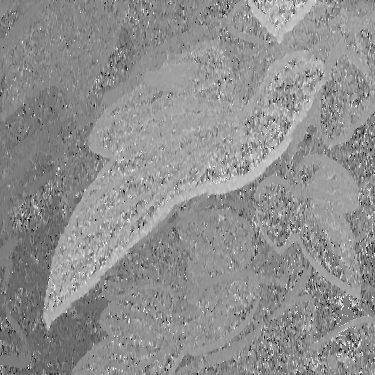
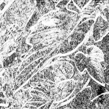
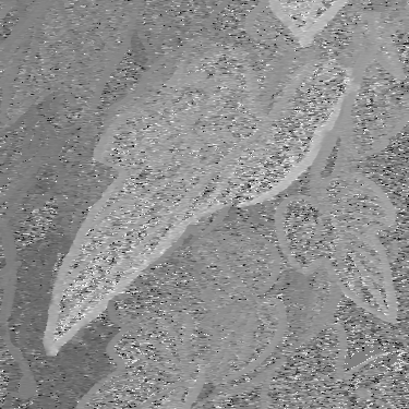
(a) depth estimation on $E_{x^{*},s^{*}}$	(b) coherence for depth estimation on $E_{x^{*},s^{*}}$	(c) depth estimation on $E_{y^{*},t^{*}}$	(d) $m_{init}$, thresholded, combined a) & c)
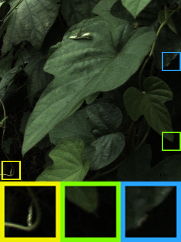
(e) center sub-aperture image	(f) smooth propagation of d)	(g) result without NLM prior	(h) result with NLM prior

Figure 1: Overview of our method on an image by [32], best viewed on screen. Note: each image was normalized to [0,1], so gray values between images may vary. Images (a)&(c) show rough depth maps, computed using the first part of the local depth estimation method of [36], (a) on the EPI $E_{x^{*},s^{*}}$, and (c) on the EPI $E_{y^{*},t^{*}}$. (b) Coherence map for the depth estimation on the EPI $E_{x^{*},s^{*}}$. (d) The two noisy depth maps are thresholded using their corresponding coherence maps and then combined. Evidently, coherent depth values are mainly located at edges while non-coherent depth values (in red) occur in smoother regions. (f) To fill the non-coherent areas, the coherent depth values are propagated using an NLM approach. (g) Our result without a prior shows more details than (f), but also introduces speckles in the depth map. (h) The NLM prior is able to get reduce speckles while preserving fine details, especially on edges.

4 Overview

Our proposed algorithm computes the depth map of a selected sub-aperture image from a light field. In this paper – without loss of generality – we choose the center sub-aperture image. Our method works in a two step procedure: as a first step, a rough estimation of the depth map is computed locally (Sec. 5). This serves as an initialization to the second step (Sec. 6), in which the estimated depth map is refined using a gradient based optimization approach.

The following implicit assumptions are made by our algorithm:

• All objects in the scene are Lambertian, a common assumption, which is also made by [38, 30, 20, 7].

• There exist no occlusions in the scene. This means that lines in the EPI images do not cross. This is a reasonable assumption, especially for the Lytro camera, as the angular resolution is not very large, as also stated by [10, 9].

• Object boundaries in the depth image coincide with changes in the RGB image. This assumption is also explicitly made in [27, 14].

Note that these assumptions are not perfectly met in real scenes. Despite relying implicitly on these assumptions, our algorithm works well on real world images as we will demonstrate in Sec. 8.

5 Rough depth map estimation using NLM

To get an initialization for the depth map, we adopt the initial part of the depth estimation algorithm of [36]: the local depth estimation on EPIs. It estimates the slopes of the lines visible in the epipolar image using the structure tensor of the EPI. It only uses the epipolar images of the angular center row ($E_{y,t^{*}}$ with $t^{*}=T/2$, $y=\{1,\ldots Y\}$) and angular center column ($E_{x,s^{*}}$ with $s^{*}=S/2$, $x=\{1,\ldots X\}$) and yields two rough depth estimates for each pixel in the center image, see Fig. 1 (a,c). Additionally, it returns a coherence map $C(\cdot)$ that provides a measure for the certainty of the estimated depth values (Fig. 1 (b)).

This approach returns consistent estimates at image edges but provides quite noisy and unreliable estimates at smoother regions, see Fig. 1 (a,c). We take the two noisy depth estimates and threshold them by setting depth values with a low coherence value to non-defined. This gives us an initial estimate for the depth values at the edges. After thresholding, the two estimates are combined: if both estimates on $E_{y,t^{*}}$ and $E_{x,s^{*}}$ for a pixel in the depth map have coherent values, we will take the depth estimation with the higher coherence value. The result is shown in Fig. 1 (d). This rough depth map estimate is denoted by $m_{init}$.

To propagate depth information into regions of non-coherent pixels (red pixels in Fig. 1 (d)), we solve the optimization problem

$$\operatornamewithlimits{argmin}_{m}\sum\limits_{p}\sum\limits_{q\in N(p)}w_{pq}\biggl{[}\,\,\big{(}m(p)-m(q)\big{)}^{2}+\,C(p)\,\big{(}m_{init}(p)-m(q)\big{)}^{2}\biggr{]}$$ (1)

where $w_{pq}\in[0,1]$ is a weighting term on the RGB image that captures the similarity of the color and gradient values of the $3\times 3$ window around $p$ and $q$ (see Sec. 6.1, Eq. (2)). $N(p)$ are the neighboring pixels around $p$, e.g. in an $11\times 11$ window with $p$ in the center. The term $w_{pq}(m(p)-m(q))^{2}$ ensures that pixels in $N(p)$ have similar depth values as $p$ if they are similar in the RGB image (high $w_{pq}$). The term $w_{pq}C(p)(m(q)-m_{init}(p))^{2}$ enforces that a pixel with high coherence $C(p)$ propagates its depth value $m_{init}(p)$ to neighboring pixels $q$ which are similar in the RGB image. Fig. 1(f) shows the result of this propagation step. Eq. (1) is minimized using L-BFGS-B [6].

(a) Overview of the refinement step visualized with sub-aperture images, best viewed on screen: The estimated light field (LF) is constructed by shifting pixels from the center sub-aperture image to the other sub-aperture images. The shifting depends on the current depth value of the shifted pixel and the distance to the sub-aperture image. The objective is to minimize the squared L2 distance between the estimated LF and the original LF.

(b) Top: Original EPI $E_{y^{*},t^{*}}$ from 7 sub-aperture images using the row in each image, which is highlighted in red above. Bottom: Estimated EPI constructed solely from the center row by shifting center row pixels according to their depth values. Note that for better visualization, the EPI’s are vertically stretched to twice their heights. Four red lines are overlaid to visualize the emergence of lines in the EPI.

(c) Overview of the refinement step visualized with an EPI.

Figure 2: Overview of the refinement step.

6 Refinement step

The refinement step is based on the observation that the sub-aperture images can be almost entirely explained and predicted from the center image $I:=I_{S/2,T/2}$ alone, namely by shifting the pixels from the image $I$ along the lines visible in the epipolar image. This has already been observed by others [16, 19, 41]. Fig. 2c visualizes the case for an EPI $E_{y^{*},t^{*}}$.

To make full use of the recorded 4D light field, the center image pixels are not only moved along a line, but along a 2D plane. For a fixed $s^{*}$ or $t^{*}$ this 2D plane becomes a line visible in the respective EPI views $E_{x^{*},s^{*}}$ or $E_{y^{*},t^{*}}$. Note that the slopes of the line $m_{x_{c},y_{c}}$ going through the center pixel $(x_{c},y_{c})$ are the same in $E_{y_{c},t^{*}}$ and $E_{x_{c},s^{*}}$.

When moving a center image pixel $I(x_{c},y_{c})$ along the 2D plane with given slope $m_{x_{c},y_{c}}$, its new coordinates in the sub-aperture image $I_{S/2+d_{s},T/2+d_{t}}$ become $(x_{c}+m_{x_{c},y_{c}}d_{s},y_{c}+m_{x_{c},y_{c}}d_{t})$, where $d_{s}$ and $d_{t}$ denote the angular distances from the center sub-aperture image to the target sub-aperture image, formally ${d_{s}=s-S/2}$, ${d_{t}=t-T/2}$. The estimated light field that arises from shifting pixels from the center sub-aperture image to all other sub-aperture views is denoted by $\widetilde{L}_{m}(s,t,x,y)$.

The influence of pixel $I(x_{c},y_{c})$ on pixel $\widetilde{L}_{m}(s,t,x,y)$ is determined by the distances $x-(x_{c}+m_{x_{c},y_{c}}d_{s})$ and $y-(y_{c}+m_{x_{c},y_{c}}d_{t})$. Only if the absolute values of both distances are smaller than one, the pixel $I(x_{c},y_{c})$ influences $\widetilde{L}_{m}(s,t,x,y)$, see Fig. 3. Any pixel in the light field $\widetilde{L}_{m}(s,t,x,y)$ can thus be computed as the weighted sum of all pixels from the center image $I$:

$$\widetilde{L}_{m}(s,t,x,y)=\sum\limits_{x_{c}}\sum\limits_{y_{c}}I(x_{c},y_{c})\cdot\Lambda\big{(}x-(x_{c}+m_{x_{c},y_{c}}d_{t})\big{)}\cdot\Lambda\big{(}y-(y_{c}+m_{x_{c},y_{c}}d_{s})\big{)}$$

where $\Lambda:\mathbb{R}\to[0,1]$ is a weighting function and denotes the differentiable version of the triangular function defined as

$$\bar{\Lambda}(x)=\begin{cases}1+x&\mbox{if }-1<x<0\\ 1-x&\mbox{if }0\leq x<1\\ 0&\mbox{otherwise, i.e. if }|x|\geq 1\end{cases}$$

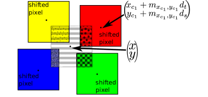
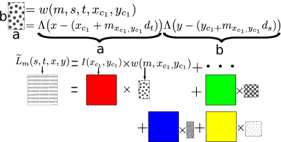
Figure 3: Modified Bilinear Interpolation: The color of the estimated pixel is determined by using a weighted sum of the shifted pixels that overlap with it. The weight of each pixel is the area of overlap with the estimated pixel.

To allow for sub-pixel shifts, we use the following bilinear interpolation scheme: As shown in Fig. 3, the intensity value of the pixel $\widetilde{L}_{m}(s,t,x,y)$ is the weighted sum of all overlapping pixels (the four colored pixels in Fig. 3). The weight of each pixel is the area of overlap with the pixel $\widetilde{L}_{m}(s,t,x,y)$, which is given by the triangular term.

Note that in practice, it is not necessary to iterate over all pixels in the center image for every pixel $\widetilde{L}_{m}(s,t,x,y)$. Instead, the projection of each pixel in the center image is calculated and added to the (up to) 4 pixels in the subview where the overlapping area is nonzero, leading to a linear runtime complexity in the size of the light field. To get a refined depth estimation map we optimize the following objective function:

$$m=\operatornamewithlimits{argmin}_{m}||\widetilde{L}_{m}-L||^{2}_{2}+\lambda\,R(m)$$

where $R(m)$ is a regularization term which we will describe in more detail in the remainder of this section.

6.1 Non-local means regularization

The NLM regularizer was first proposed in [5] and has proven useful for the refinement of depth maps in other contexts [13]. We define it as

$$R(m)=\sum\limits_{p}\sum\limits_{q\in N(p)}w_{pq}(m(p)-m(q))^{2}$$

with $N(p)$ being the search window around a pixel $p$, e.g. an $11\times 11$ window, and $w_{pq}$ is the weight expressing the similarity of the pixels $p$ and $q$. We define $w_{pq}$ as

$$w_{pq}=\exp\Bigg{(}-\mathop{\sum_{p^{\prime}\in N^{\prime}(p)}}_{q^{\prime}\in N^{\prime}(q)}\frac{[I(p^{\prime})-I(q^{\prime})]^{2}}{\sigma_{Color}^{2}}+\frac{[\nabla_{p,p^{\prime}}I-\nabla_{q,q^{\prime}}I]^{2}}{\sigma_{Grad}^{2}}\Bigg{)}$$ (2)

where $\sigma_{Color}^{2}$ and $\sigma_{Grad}^{2}$ are the variances in the color and gradient values of the image and $\nabla_{p,p^{\prime}}I:=I(p)-I(p^{\prime})$ is the image gradient at pixel position $p$. This encourages edges in the depth map at locations where edges exist in the RGB image and smoothens out the remaining regions. In all experiments, $N^{\prime}$ was a $3\times 3$ window.

7 Implementation Details

Our implementation is in MATLAB. For numerical optimization we used the MATLAB interface by Peter Carbonetto [6] of the gradient based optimizer L-BFGS-B [42]. The only code-wise optimization we applied is implementing some of the computationally expensive parts (light field synthesis) in C (MEX) using the multiprocessing API OpenMP. Current runtime for computing the depth map from the $7\times 7\times 375\times 375\times 3$ light field from the Lytro camera is about 270 seconds on a 64bit Intel Xeon CPU E5-2650L 0 @ 1.80GHz architecture using 8 cores. All parameter settings for the experiments are included in the supplementary and in the source code and are omitted here for brevity. In particular, we refer the interested reader to the supplementary for explanations of their influence to the depth map estimation along with reasonable ranges that work well for different types of images. The code as well as our Lytro dataset is publicly available.

8 Experimental results

Comparison on Lytro images

In Fig. 4 we show a comprehensive comparison of our results with several other works including the recent work of [35] and [24]. The resolution of the Lytro light field is $S\times T=7\times 7$, and the resolution of each sub-aperture image is $X\times Y=375\times 375$ pixels. We decoded the raw Lytro images with the algorithm by [11], whereas others have developed proprietary decoding procedures leading to slightly different image dimensions.

Overall, our algorithm is able to recover more details and better defined edges while introducing no speckles to the depth maps. Depth variations on surfaces are much smoother in our results than e.g. in [35] or [24] while being able to preserve sharp edges. Even small details are resolved in the depth map, see e.g. the small petiole in the lower left corner of the leaf image (second row from the top, not visible in print).

Reference	Our results	[32]	[35]	[24]	[31]	[36]

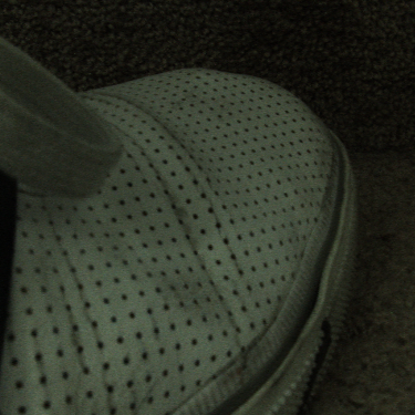
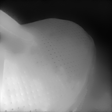
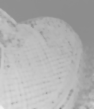
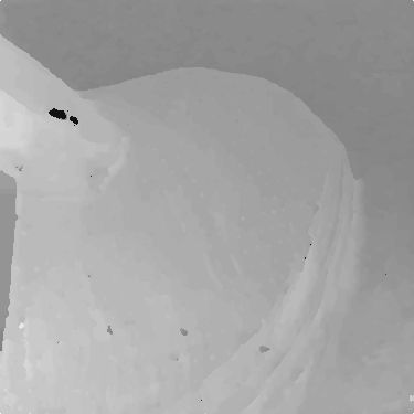
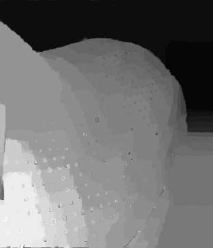
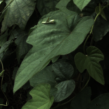
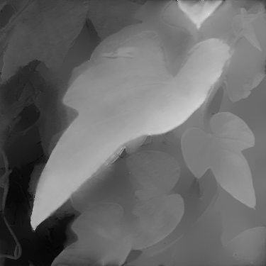
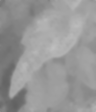
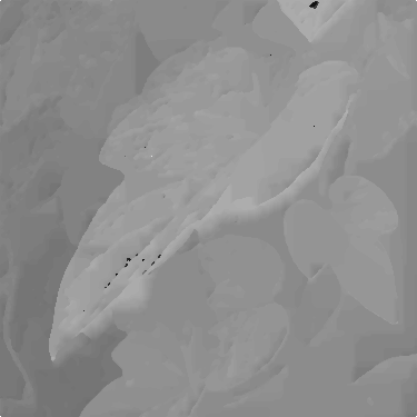
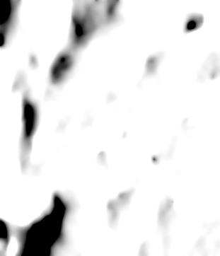
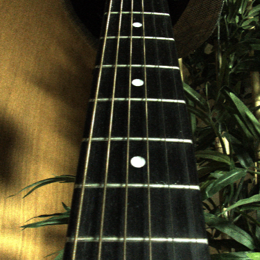
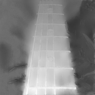
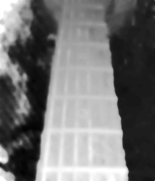
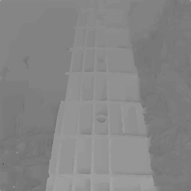
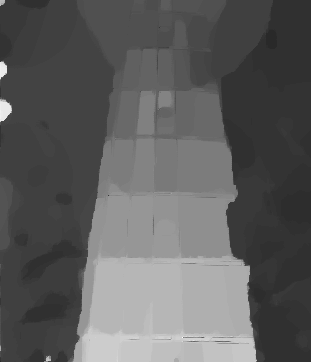
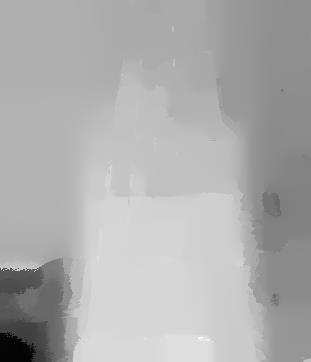
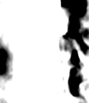
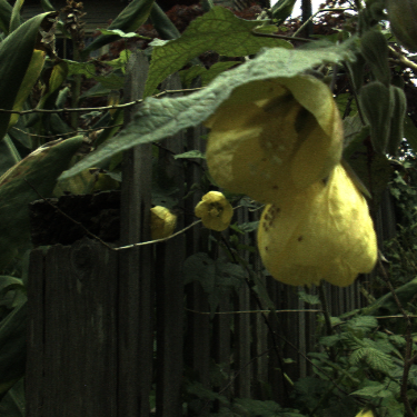
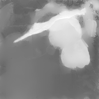
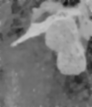
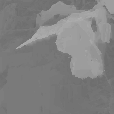
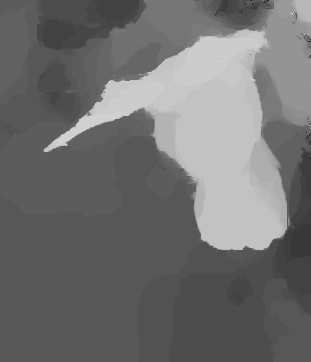
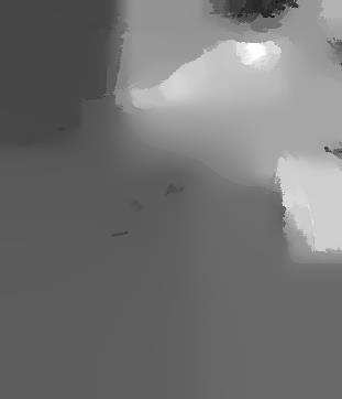
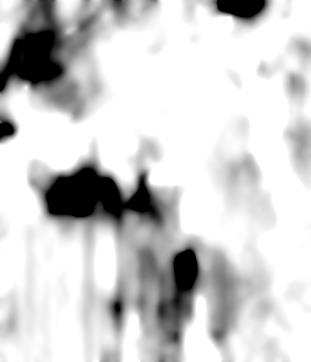
Figure 4: Comparison on Lytro images taken from [32], best viewed on screen. The results for [31] and [36] are taken from [24]. Our algorithm is able to recover finer details and produces fewer speckles in the depth map. Note that [31] is originally an optical flow algorithm whose results are included for comparison.

Comparison on the Stanford light field dataset

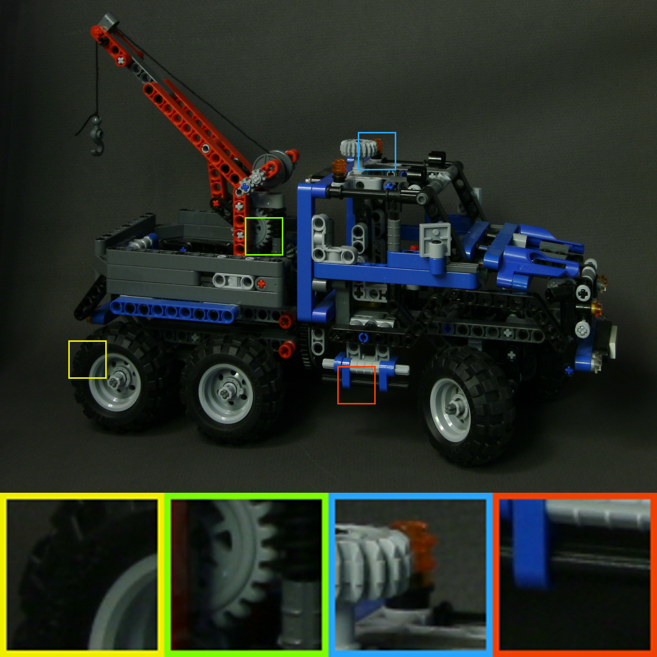
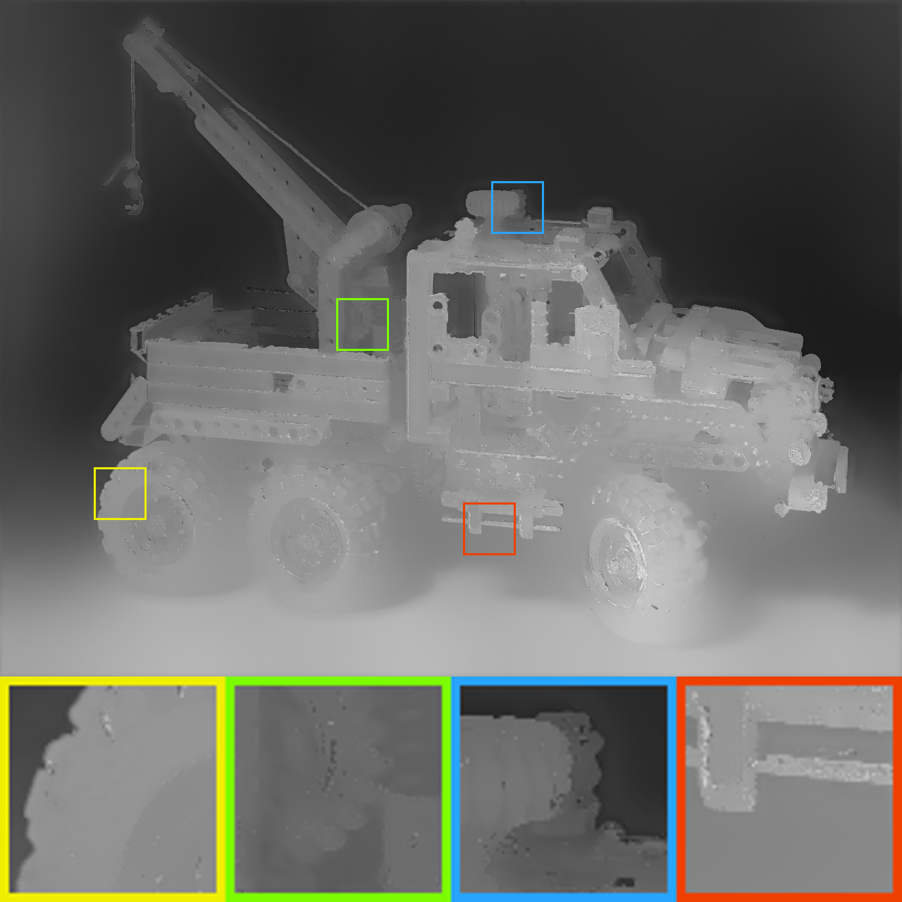
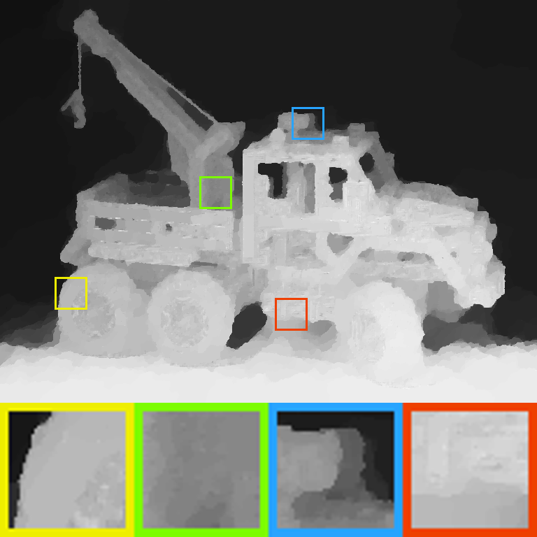
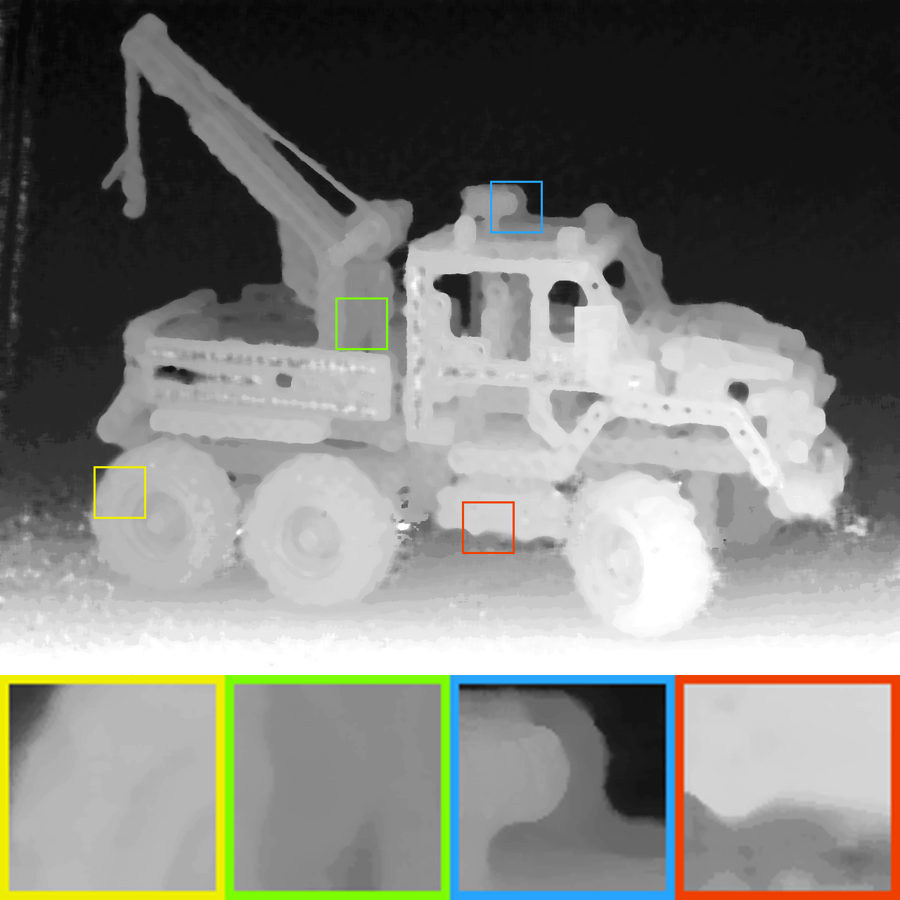
(a) center image	(b) our result	(c) result of [36]	(d) result of [20]

Figure 5: Comparison on images of the Stanford light field dataset [1], best viewed on screen. We are able to recover finer details and our depth boundaries match better with the RGB image boundaries. The resolution is $1280\times 960$ for all images except for [36], where it is $768\times 576$ as the image is taken from the respective paper.

In Fig. 5 we compare our method on the truck image of the Stanford light field dataset [1]. The light field has a resolution of $S\times T=17\times 17$ sub-aperture views. Each sub-aperture image has a resolution of $X\times Y=1280\times 960$ pixels. Compared to the already visually pleasing results of [36] and [20], we are able to recover finer and more accurate details (see closeups in Fig. 5). Additionally, the edges of the depth map match better with the edges of the RGB image. The results on the Amethyst image and further comparisons are shown in the supplementary.

Quantitative evaluation on artificial dataset

We compare our algorithm with the state of the art [35] on the artificial dataset provided by [39]. We could not reproduce the given numerical results, so we used the provided code for the comparison. The average root mean square error on the whole dataset is 0.067 for [35] and 0.063 for our algoritm. The depth maps and further details are given in the supplementary.

9 Conclusion and future work

We presented a novel approach to estimate the depth map from light field images. A crucial ingredient of our approach is a generative model for light field images which can also be used for other image processing tasks on light fields. Our approach consists of two steps. First, a rough initialization of the depth map is computed. In the second step, this initialization is refined by using a gradient based optimization approach.

We have evaluated our approach on a light field image from the Stanford dataset [1], on real-world images taken with a Lytro camera and on artificially generated light field images. Despite the Lytro images being rather noisy, our recovered depth maps exhibit fine details with well-defined boundaries.

Our work can be extended and improved in several directions. The algorithm lends itself well to parallelization and seems ideally suited for a GPU implementation. Another interesting direction is to modify our generative light field model to explicitly account for occlusions. While our forward model can be readily adapted to allow for cross-sections in the EPI, optimization becomes more intricate. We leave a solution to this problem for future work.

References

- [1] The (new) stanford light field archive. http://lightfield.stanford.edu (2008), [Online; accessed 07-April-2016]
- [2] Adelson, E.H., Wang, J.Y.A.: Single lens stereo with a plenoptic camera. IEEE Transactions on Pattern Analysis and Machine Intelligence (PAMI) 14(2), 99–106 (1992)
- [3] Bishop, T.E., Favaro, P.: The light field camera: Extended depth of field, aliasing, and superresolution. IEEE Transactions on Pattern Analysis and Machine Intelligence (PAMI) 34(5), 972–986 (2012)
- [4] Bolles, R.C., Baker, H.H., Marimont, D.H.: Epipolar-plane image analysis: An approach to determining structure from motion. International Journal of Computer Vision 1(1), 7–55 (1987)
- [5] Buades, A., Coll, B., Morel, J.M.: A non-local algorithm for image denoising. In: CVPR (2005)
- [6] Carbonetto, P.: A programming interface for L-BFGS-B in MATLAB. https://github.com/pcarbo/lbfgsb-matlab (2014), [Online; accessed 15-April-2015]
- [7] Chai, J.X., Tong, X., Chan, S.C., Shum, H.Y.: Plenoptic sampling. In: ACM SIGGRAPH (2000)
- [8] Cho, D., Kim, S., Tai, Y.W.: Consistent matting for light field images. In: ECCV (2014)
- [9] Dansereau, D.G., Bongiorno, D.L., Pizarro, O., Williams, S.B.: Light field image denoising using a linear 4D frequency-hyperfan all-in-focus filter. In: IS&T/SPIE Electronic Imaging (2013)
- [10] Dansereau, D.G., Mahon, I., Pizarro, O., Williams, S.B.: Plenoptic flow: Closed-form visual odometry for light field cameras. In: IROS (2011)
- [11] Dansereau, D.G., Pizarro, O., Williams, S.B.: Decoding, calibration and rectification for lenselet-based plenoptic cameras. In: CVPR (2013)
- [12] Diebold, M., Goldlücke, B.: Epipolar plane image refocusing for improved depth estimation and occlusion handling. In: Annual Workshop on Vision, Modeling and Visualization: VMV (2013)
- [13] Favaro, P.: Recovering thin structures via nonlocal-means regularization with application to depth from defocus. In: CVPR (2010)
- [14] Ferstl, D., Reinbacher, C., Ranftl, R., Rüther, M., Bischof, H.: Image guided depth upsampling using anisotropic total generalized variation. In: ICCV (2013)
- [15] Goldluecke, B., Wanner, S.: The variational structure of disparity and regularization of 4D light fields. In: CVPR (2013)
- [16] Gortler, S.J., Grzeszczuk, R., Szeliski, R., Cohen, M.F.: The lumigraph. In: ACM SIGGRAPH (1996)
- [17] Heber, S., Pock, T.: Shape from light field meets robust PCA. In: ECCV (2014)
- [18] Heber, S., Ranftl, R., Pock, T.: Variational shape from light field. In: Energy Minimization Methods in Computer Vision and Pattern Recognition. Springer (2013)
- [19] Isaksen, A., McMillan, L., Gortler, S.J.: Dynamically reparameterized light fields. In: ACM SIGGRAPH. ACM (1996)
- [20] Kim, C., Zimmer, H., Pritch, Y., Sorkine-Hornung, A., Gross, M.H.: Scene reconstruction from high spatio-angular resolution light fields. ACM SIGGRAPH (2013)
- [21] Levoy, M., Hanrahan, P.: Light field rendering. In: ACM SIGGRAPH. ACM (1996)
- [22] Li, N., Ye, J., Ji, Y., Ling, H., Yu, J.: Saliency detection on light field. In: CVPR (2014)
- [23] Liang, C.K., Lin, T.H., Wong, B.Y., Liu, C., Chen, H.H.: Programmable aperture photography: multiplexed light field acquisition. ACM SIGGRAPH (2008)
- [24] Lin, H., Chen, C., Bing Kang, S., Yu, J.: Depth recovery from light field using focal stack symmetry. In: ICCV (2015)
- [25] Ng, R.: Digital light field photography. Ph.D. thesis, stanford university (2006), [Ren Ng founded Lytro]
- [26] Ng, R., Levoy, M., Brédif, M., Duval, G., Horowitz, M., Hanrahan, P.: Light field photography with a hand-held plenoptic camera. Computer Science Technical Report CSTR 2(11) (2005)
- [27] Park, J., Kim, H., Tai, Y.W., Brown, M.S., Kweon, I.: High quality depth map upsampling for 3D-TOF cameras. In: ICCV (2011)
- [28] Perwass, C., Wietzke, L.: The next generation of photography. https://github.com/pcarbo/lbfgsb-matlab (2010), [Online; accessed 15-April-2015; Perwass and Wietzke founded Raytrix]
- [29] Perwass, C., Wietzke, L.: Single lens 3D-camera with extended depth-of-field. In: IS&T/SPIE Electronic Imaging (2012)
- [30] Sebe, I.O., Ramanathan, P., Girod, B.: Multi-view geometry estimation for light field compression. In: Annual Workshop on Vision, Modeling and Visualization: VMV (2002)
- [31] Sun, D., Roth, S., Black, M.J.: Secrets of optical flow estimation and their principles. In: CVPR (2010)
- [32] Tao, M.W., Hadap, S., Malik, J., Ramamoorthi, R.: Depth from combining defocus and correspondence using light-field cameras. In: ICCV (2013)
- [33] Tosic, I., Berkner, K.: Light field scale-depth space transform for dense depth estimation. In: CVPR Workshops (2014)
- [34] Vaish, V., Wilburn, B., Joshi, N., Levoy, M.: Using plane+ parallax for calibrating dense camera arrays. In: CVPR (2004)
- [35] Wang, T.C., Efros, A.A., Ramamoorthi, R.: Occlusion-aware depth estimation using light-field cameras. In: ICCV (2015)
- [36] Wanner, S., Goldluecke, B.: Globally consistent depth labeling of 4D light fields. In: CVPR (2012)
- [37] Wanner, S., Goldluecke, B.: Spatial and angular variational super-resolution of 4D light fields. In: ECCV (2012)
- [38] Wanner, S., Goldluecke, B.: Variational light field analysis for disparity estimation and super-resolution. IEEE Transactions on Pattern Analysis and Machine Intelligence (PAMI) 36(3), 606–619 (2014)
- [39] Wanner, S., Meister, S., Goldluecke, B.: Datasets and benchmarks for densely sampled 4d light fields. In: Annual Workshop on Vision, Modeling and Visualization: VMV (2013)
- [40] Wanner, S., Straehle, C., Goldluecke, B.: Globally consistent multi-label assignment on the ray space of 4D light fields. In: CVPR (2013)
- [41] Zhang, Z., Liu, Y., Dai, Q.: Light field from micro-baseline image pair. In: CVPR (2015)
- [42] Zhu, C., Byrd, R.H., Lu, P., Nocedal, J.: Algorithm 778: L-BFGS-B: Fortran subroutines for large-scale bound-constrained optimization. ACM TOMS 23(4), 550–560 (1997)