Trochoidal trajectories of self-propelled Janus particles in a diverging laser beam

Abstract

We describe colloidal Janus particles with metallic and dielectric faces that swim vigorously when illuminated by defocused optical tweezers without consuming any chemical fuel. Rather than wandering randomly, these optically-activated colloidal swimmers circulate back and forth through the beam of light, tracing out sinuous rosette patterns. We propose a model for this mode of light-activated transport that accounts for the observed behavior through a combination of self-thermophoresis and optically-induced torque. In the deterministic limit, this model yields trajectories that resemble rosette curves known as hypotrochoids.

I Introduction

Colloidal particles that consume fuel to translate and rotate are important examples of active matter Golestanian et al. (2005); Marchetti et al. (2013). Typically taking the form of bifunctional Janus particles Walther and Müller (2008), such colloidal swimmers are driven by gradients of concentration and temperature that result from chemical reactions Paxton et al. (2004); Golestanian et al. (2005). Several examples of light-activated colloidal swimmers have been reported whose motions are driven by thermophoresis Jiang et al. (2010); Volpe et al. (2011); Buttinoni et al. (2012, 2013); Qian et al. (2013). This mode of motion recently has been analyzed theoretically Bickel et al. (2014). Here, we describe experimental studies of the motion of light-activated colloidal swimmers in nonuniform light fields. The interplay of thermophoresis and optical forces in this system gives rise to highly structured single-particle trajectories resembling the class of rosette curves known as trochoids.

I.1 Light-activated swimmers

Our experimental system, shown schematically in Figure 1(a), consists of a colloidal particle illuminated by a diverging laser beam. Each bifunctional particle is comprised of a $300\text{\,}\mathrm{nm}$-wide hematite cube partially embedded in the surface of a $2\text{\,}\mathrm{\SIUnitSymbolMicro m}$-diameter sphere made of 3-methacryloxypropyl trimethoxysilane (TPM) Sacanna et al. (2012); Abrikosov et al. (2013); Palacci et al. (2013, 2014). The bright-field microscope image in Figure 1(b) shows a typical particle with its cube visible on the left side. These particles are dispersed in deionized water at a volume fraction of ${10}^{-5}$, with $5\text{\,}\mathrm{mM}$ tetramethylammonium hydroxide (TMAH) added to increase the pH to $8.5$. Raising the pH prevents the spheres from sticking to the glass walls of their container, which is made from a $2\text{\,}\mathrm{cm}$-long glass capillary with cross-section area $$1\text{\,}\mathrm{mm}$\times$100\text{\,}\mathrm{\SIUnitSymbolMicro m}$$ (Vitrocom, catalog number 5010). Both TPM and hematite are substantially denser than water, and the composite particles rapidly sediment to the bottom wall, as depicted in Figure 1(a).

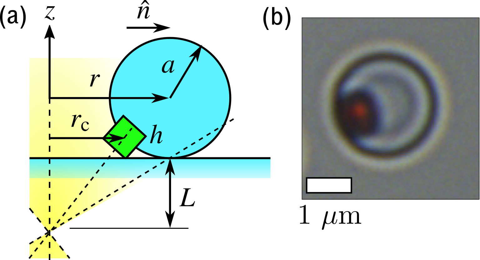
Figure 1: (a) Schematic representation of a hematite-TPM composite particle being illuminated by a diverging laser beam as it rests on a horizontal glass surface. (b) Bright-field image of a $2\text{\,}\mathrm{\SIUnitSymbolMicro m}$-diameter swimmer. Scale bar indicates $1\text{\,}\mathrm{\SIUnitSymbolMicro m}$.

TPM is a transparent dielectric at optical wavelengths. Hematite, by contrast, absorbs visible light strongly. When a composite particle is illuminated, its hematite side becomes warmer than its TPM side. The local temperature gradient gives rise to thermophoresis, which causes the particle to move Weinert and Braun (2008); Jiang et al. (2010); Yang and Ripoll (2013). In uniform illumination, this motion is essentially ballistic, with rotational diffusion causing small deviations in a swimmer’s trajectory Jiang et al. (2010); Bickel et al. (2014). Here, we show that nonuniform illumination engenders motion of a very different nature, with the particle tracing out continuous loops that pass through the intensity maximum and turn around near the periphery of the light field. This behavior differs from previous reports of thermophoretic swimmers in optical traps Jiang et al. (2010) whose trajectories appeared diffusive.

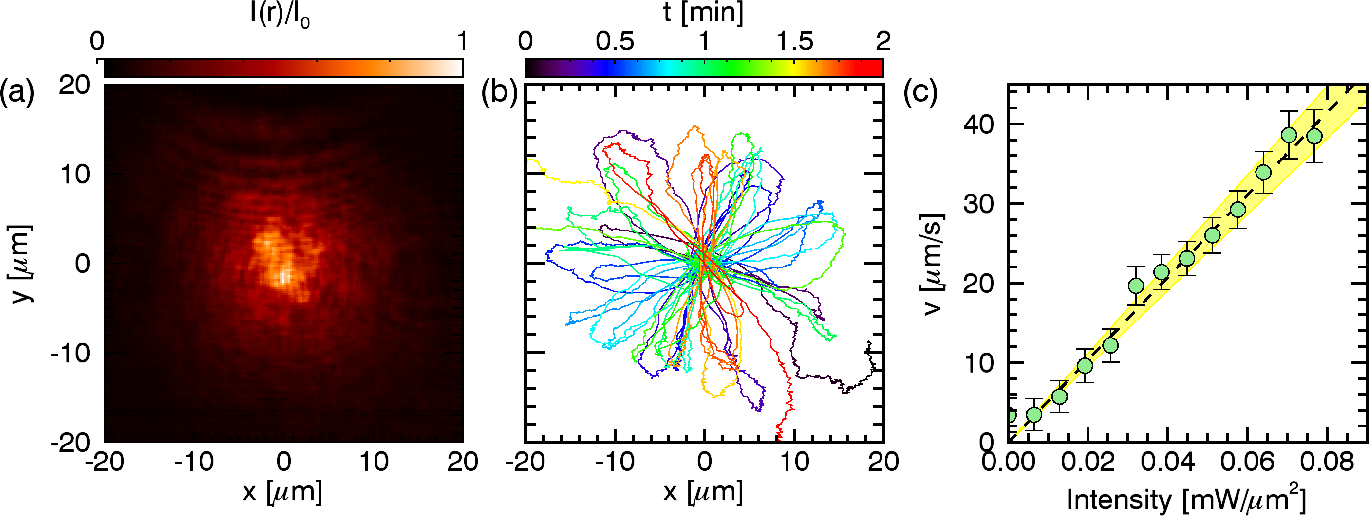
Figure 2: (a) Measured intensity distribution $I(\mathbf{r})$ of laser illumination in the plane of the swimmer’s motion. The color bar indicates values relative to the peak value, $I_{0}$, at the center. (b) Two minutes of a typical swimmer’s trajectory colored by time. The trajectory loops repeatedly through the center of the intensity distribution. (c) Relationship between the swimming speed, $v(\mathbf{r})$, and the local light intensity, $I(\mathbf{r})$. The dashed line is a one-parameter fit for the associated mobility, $\alpha=$518\pm 41.\text{\,}{\mathrm{\SIUnitSymbolMicro m}}^{3}\text{\,}{\mathrm{s}}^{-1}\text{\,}{\mathrm{mW}}^{-1}$$.

I.2 Illumination and imaging

Our instrument consists of an inverted holographic optical trapping system that operates at a vacuum wavelength of $532\text{\,}\mathrm{nm}$ (Coherent Verdi) and creates patterns of optical tweezers with computer-generated holograms that are imprinted onto the laser beam with a liquid-crystal spatial light modulator (Hamamatsu X13267-04 LCoS SLM). These holograms are projected into the sample using a microscope objective lens (Nikon Plan-Apo $60\times$, numerical aperture 1.4, oil immersion). The single trap used for this study was powered with $0.6\text{\,}\mathrm{W}$ at the laser’s output, which corresponds to roughly $0.1\text{\,}\mathrm{W}$ delivered to the sample.

The same objective lens is used to relay images of swimmers interacting with the optical traps onto an integrated video camera (NEC TI-324A), which records them at even time intervals of $\tau=$33.3\text{\,}\mathrm{ms}$$. The microscope’s $$90\text{\,}\mathrm{\SIUnitSymbolMicro m}$\times$70\text{\,}\mathrm{\SIUnitSymbolMicro m}$$ field of view typically contains one particle. Images are analyzed with standard methods of digital video microscopy Crocker and Grier (1996); Krishnatreya and Grier (2014) to measure a swimmer’s trajectory, $\mathbf{r}_{n}=\mathbf{r}(t_{n})$ at times $t_{n}=n\tau$ that are integer multiples of the frame interval. Because the particle remains sedimented onto the lower glass surface with its hematite cube inclined downward, we can define its orientation $\hat{n}(t)$ to be directed from the center of the cube to the center of the sphere along the horizontal plane.

The illuminated particle swims in the direction of $\hat{n}(t)$, which is to say away from its hotter end. This differs from these particles’ motion in the presence of hydrogen peroxide Palacci et al. (2013, 2014). In this case, decomposition of the chemical fuel engenders osmotic flows that propel the particle in the opposite direction. In both cases, the phoretic flow responsible for propulsion does not lift the swimmers off the lower glass surface; their motions are essential two-dimensional.

Rather than focusing an optical trap onto such a particle, we instead focus it $L\approx$10\text{\,}\mathrm{\SIUnitSymbolMicro m}$$ below the lower glass surface, as indicated in Figure 1(a), so that the colloidal particle is illuminated by a diverging beam that propagates upward and outward. Figure 2(a) shows the intensity distribution, $I(\mathbf{r})$, in the plane of the particle that is measured by replacing the sample with a front-surface mirror in the same plane. This distribution is well described by a Gaussian surface of revolution,

$$I(\mathbf{r})=I_{0}\,\exp\left(-\frac{r^{2}}{2\sigma^{2}}\right),$$ (1)

with width $\sigma=$7.3\pm 0.2\text{\,}\mathrm{\SIUnitSymbolMicro m}$$.

I.3 Trajectory analysis

As soon as the particle is illuminated, it starts to translate across the lower glass wall of its container. The data in Figure 2(b) show a typical $2\text{\,}\mathrm{min}$ trajectory. The swimmer’s trajectory is localized around the center of brightness and has a looping character that is quite distinct from Brownian motion. The trajectory curves gently as the swimmer passes through the center of the laser beam, and loops back around at the beam’s periphery to create a rosette pattern. Thermal randomness is evident in the trajectory’s small deviations. The coherent large-scale motion, however, suggests the action of an underlying deterministic process. Comparable behavior is observed for all particles in the sample; the example in Figure 2(b) is typical. This motion continues for several minutes at a time, and ends when the particle eventually moves out of the light and stops moving altogether.

We estimate the swimmer’s instantaneous velocity from the measured trajectory as

$$\mathbf{v}_{n}=\frac{\mathbf{r}_{n}-\mathbf{r}_{n-1}}{\tau}$$ (2)

at the mid-point position

$$\bar{\mathbf{r}}_{n}=\frac{1}{2}(\mathbf{r}_{n}+\mathbf{r}_{n-1}).$$ (3)

The trajectory-averaged position dependence of the swimmer’s speed then can be computed from the $N$-point trajectory using an adaptive kernel density estimator Silverman (1992),

$$v(\mathbf{r})=\frac{1}{\sqrt{2}(N-1)\rho(\mathbf{r})}\sum_{n=2}^{N}\frac{v_{n}}{\sigma_{n}}\,\exp\left(-\frac{\left|\mathbf{r}-\bar{\mathbf{r}}_{n}\right|^{2}}{2\sigma_{n}^{2}}\right),$$ (4)

whose width $\sigma_{n}$ is selected based on the density of measurements. The speed estimate is normalized by the density of measurements,

$$\rho(\mathbf{r})=\frac{1}{\sqrt{2}(N-1)}\sum_{n=2}^{N}\frac{1}{\sigma_{n}}\exp\left(\frac{\left|\mathbf{r}-\bar{\mathbf{r}}_{n}\right|^{2}}{2\sigma_{n}^{2}}\right).$$ (5)

The data in Figure 2(c) show how the swimming speed depends on the local light intensity obtained by combining results for $v(\mathbf{r})$ with those for $I(\mathbf{r})$. The swimmer moves most rapidly as it passes through the center of the beam, where the light is brightest.

II Self-thermophoretic swimming

We propose that the swimmer moves through the light field primarily by self-thermophoresis engendered by optically-induced heating. Specifically, the hematite cube’s temperature rises as it absorbs light from the beam. The resulting temperature gradient, $\nabla T(\mathbf{r})$, then induces motion through thermophoresis with a drift velocity,

$$\mathbf{v}(\mathbf{r})=D_{T}\,\nabla T(\mathbf{r}).$$ (6)

The thermal diffusion coefficient, $D_{T}$, depends on the properties of the species dissolved in the solvent Iacopini et al. (2006); Yang and Ripoll (2013), and presumably is dominated by TMAH. When dispersed in solutions without TMAH, these particles still move under laser illumination, but at only a tenth of the speed. The resulting trajectories are far more strongly influenced by both rotational and translational Brownian motion and lack the looping nature of the trajectory plotted in Figure 2(b). This is consistent with previous studies of bulk thermophoresis in which added salt is found to play a similar role Fayolle et al. (2008).

Unlike previous studies of particle motion in externally-imposed temperature gradients Yang and Ripoll (2013), the temperature gradient in this system is generated at the position of the particle through optically-induced heating of the hematite cube. Both $T(\mathbf{r})$ and $\nabla T(\mathbf{r})$ vary as the particle moves through $I(\mathbf{r})$. Previous reports suggest that $D_{T}$ may be largely independent of the temperature Iacopini et al. (2006); Yang and Ripoll (2013). In that case, we might expect the swimmer’s translation speed $v(\mathbf{r})$ to be proportional to the local intensity, $I(\mathbf{r})$. A straightforward model for the swimmer’s motion is therefore

$$\mathbf{v}(\mathbf{r})=\alpha\,I(\mathbf{r})\,\hat{n},$$ (7)

where $\hat{n}$ denotes the orientation of the swimmer from the center of the cube to center of the sphere, as indicated in Figure 1(a). The dashed line superimposed on the data in Figure 2(c) is a one-parameter fit to Eq. (7) with $\alpha=$518\pm 41.\text{\,}\mathrm{{}^{3}}{\mathrm{\SIUnitSymbolMicro}\mathrm{m}}\mathrm{/}\mathrm{s}\,\mathrm{m}\mathrm{W}$$. Without a direct probe of the local temperature, however, the relationship between $I(\mathbf{r})$ and $\nabla T(\mathbf{r})$ is difficult to gauge, which precludes using $\alpha$ to estimate $D_{T}$.

II.1 Flow field generated by a stationary swimmer

We test this model for self-thermophoretic swimming by using tracer particles to map the flow field created by a stationary swimmer that is affixed to the lower glass surface. We then compare the measured velocity field to predictions of a hydrodynamic model that accounts for the tracer particles’ own thermophoresis. Correcting for the tracers’ thermophoresis yields an estimate for the stationary swimmer’s intrinsic flow field. This, in turn, is related to the hydrodynamic forces that enable a free particle to swim.

The external force that prevents the stuck swimmer from moving is transferred to the fluid, thereby generating a flow field. Because we are primarily interested in the far-field flow profile, we model this force as a point source of flow, or stokeslet, located at the center of the swimmer and directed opposite to the orientation vector, $\hat{n}$. The Oseen tensor for this flow is Pozrikidis (1992)

$$\mathsf{{G}}_{\alpha\beta}^{S}(\mathbf{r})=\frac{1}{8\pi\eta r}\,\left(\delta_{\alpha\beta}+\frac{r_{\alpha}r_{\beta}}{r^{2}}\right),$$ (8)

where $\eta=${10}^{-3}\text{\,}\mathrm{Pa}\text{\,}\mathrm{s}$$ is the viscosity of water. The flow at position $\mathbf{r}$ due to a force $\mathbf{f}(\mathbf{r}_{0})$ acting on a particle at $\mathbf{r}_{0}$ is

$$\mathbf{u}^{S}(\mathbf{r})=\mathsf{{G}}^{S}(\mathbf{r}-\mathbf{r}_{0})\cdot\mathbf{f}(\mathbf{r}_{0}).$$ (9)

For the particular case of light-induced self-thermophoresis, the driving force acting on the fluid should be comparable to the force responsible for the free swimmer’s motion,

$$\mathbf{f}(\mathbf{r}_{0}) \approx\frac{1}{\mu}\,\mathbf{v}(\mathbf{r}_{0})$$ (10a)

$$=\frac{1}{\mu}\,\alpha\,I(\mathbf{r}_{0})\,\hat{n},$$ (10b)

where $\mu$ is the swimmer’s wall-corrected mobility. We further assume that this point force operates on the fluid at the center of the sphere.

To satisfy no-slip boundary conditions at the nearby glass surface, we adopt the method of images Blake (1971); Pozrikidis (1992), in which the flow at the surface is identically canceled by the source’s hydrodynamic image in the surface. The hydrodynamic image for the stokeslet at $\mathbf{r}_{0}$ consists of a stokeslet located at the mirror position, $\mathbf{r}_{1}=\mathbf{r}_{0}-2a\hat{z}$, and oriented in the opposite direction, plus additional contributions Blake (1971) from a source doublet (SD),

$$\mathsf{{G}}_{\alpha\beta}^{SD}(\mathbf{r})=\frac{1}{8\pi\eta r^{3}}\left(-\delta_{\alpha\beta}+3\frac{r_{\alpha}r_{\beta}}{r^{2}}\right),$$ (11)

and a stokeslet dipole (D) oriented in direction $\hat{d}=\hat{n}-2n_{z}\hat{z}$,

$$\mathsf{{G}}_{\alpha\beta}^{D}(\mathbf{r},\hat{d})=\frac{1}{8\pi\eta r^{3}}\biggl{[}\hat{d}\cdot\mathbf{r}\left(\delta_{\alpha\beta}+3\frac{r_{\alpha}r_{\beta}}{r^{2}}\right)-(r_{\alpha}d_{\beta}+r_{\beta}d_{\alpha})\biggr{]}.$$ (12)

The flow field generated by this image system is

$$\mathbf{u}^{I}(\mathbf{r}) =-\mathsf{{G}}^{S}(\mathbf{r}-\mathbf{r}_{1})\cdot\mathbf{f}(\mathbf{r}_{0})-2a^{2}\,\mathsf{{G}}^{SD}(\mathbf{r}-\mathbf{r}_{1})\cdot\hat{d}\,f(\mathbf{r}_{0})$$

$$\quad\quad+2a\,\mathsf{{G}}^{D}(\mathbf{r}-\mathbf{r}_{1},\hat{d})\cdot\hat{z}\,\mathbf{f}(\mathbf{r}_{0})\cdot\hat{z}$$ (13a)

$$=\mathsf{{G}}^{I}(\mathbf{r}-\mathbf{r}_{1})\cdot\mathbf{f}(\mathbf{r}_{0}).$$ (13b)

The total Oseen tensor for this model is then

$$\mathsf{{G}}(\mathbf{r}-\mathbf{r}_{0})=\mathsf{{G}}^{\text{S}}(\mathbf{r}-\mathbf{r}_{0})+\mathsf{{G}}^{\text{I}}(\mathbf{r}-\mathbf{r}_{1}),$$ (14)

and the total flow at position $\mathbf{r}$ is

$$\mathbf{u}(\mathbf{r})=-\alpha I(\mathbf{r}_{c})\,\mathsf{{G}}(\mathbf{r}-\mathbf{r}_{0})\cdot\hat{n}.$$ (15)

We neglect hydrodynamic coupling to the more distant parallel wall, which would add substantially to the complexity of the model Liron and Mochon (1976), but would not appreciably influence particles’ motions near the lower wall Dufresne et al. (2001).

Were the particle free to move, the reaction force, $-\mathbf{f}(\mathbf{r}_{0})$, would give rise to a stresslet flow associated with force-free motion Spagnolie and Lauga (2012). In the absence of the external restraining force, the swimmer then would move with velocity

$$\mathbf{v}(\mathbf{r})=-\mathbf{u}(\mathbf{r}).$$ (16)

II.2 Accounting for tracer thermophoresis

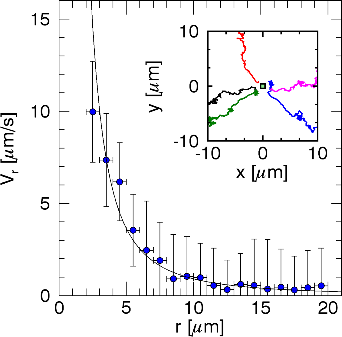
Figure 3: The measured radial speed, $V_{r}(r)$, of tracer particles approaching an illuminated hematite cube at $r=0$, computed according to Eq. (20). The solid curve is a one-parameter fit to Eq. (19). Inset: Representative trajectories of five tracer spheres drifting inward toward the stationary hematite cube.

We map the flow field, $\mathbf{u}(\mathbf{r})$, by measuring the trajectories Crocker and Grier (1996) of silica spheres of radius $a_{tr}=$150\text{\,}\mathrm{nm}$$ that are dispersed in the system as tracer particles. Their velocity, $\mathbf{V}(\mathbf{r})$, in the presence of a stationary swimmer located at $\mathbf{r}=0$ provides insight into the swimmer-induced flow field. According to Faxén’s first law, a tracer sphere of radius $a_{tr}$ immersed in a flow field $\mathbf{u}(\mathbf{r})$ and driven by an external force $\mathbf{F}(\mathbf{r})$ has an instantaneous velocity

$$\mathbf{V}(\mathbf{r})=\mathbf{u}(\mathbf{r})+\frac{a_{tr}^{2}}{6}\nabla^{2}\mathbf{u}+\mathsf{{b}}(\mathbf{r})\cdot\mathbf{F}(\mathbf{r}),$$ (17)

where $\mathsf{{b}}(\mathbf{r})$ is the sphere’s mobility tensor.

We include $\mathbf{F}(\mathbf{r})$ in Eq. (17) to account for thermophoresis of the tracer particles in the non-uniform temperature field generated by the hot hematite cube. The steady-state temperature profile around the heated cube satisfies the Laplace equation and therefore may be modeled as

$$T(\mathbf{r})=T_{\infty}+\frac{h}{r}(T_{c}-T_{\infty}),$$ (18)

where $T_{\infty}$ is the temperature far from the cube, $T_{c}$ is the cube’s temperature, and $h$ is the length of the cube’s side. Equation (18) applies in the far field, for $r>h$. A tracer particle’s thermophoretic velocity therefore should be

$$\mathsf{{b}}(\mathbf{r})\cdot\mathbf{F}(\mathbf{r})=-D_{T}^{tr}(T_{c}-T_{\infty})h\,\frac{1}{r^{2}}\hat{r},$$ (19)

where $D_{T}^{tr}$ is the tracers’ thermal diffusion coefficient. Thermophoresis causes the tracers to drift inward toward the cube.

To test this model and to estimate the relevant coefficients, we measure tracer particles’ trajectories in the presence of bare hematite cubes stuck to the lower glass wall. This isolates the drift due to tracer thermophoresis from the flow due to the swimmer’s self-thermophoresis. Figure 3 shows the ensemble average of tracers’ measured radial speeds,

$$V_{r}(r)=\frac{1}{2\pi}\int_{0}^{2\pi}\left|\mathbf{V}(\mathbf{r})\cdot\hat{r}\right|\,d\theta,$$ (20)

averaged over angles centered on the heated cube. Typical trajectories are plotted in the inset to Figure 3. The solid curve in Figure 3 is a one-parameter fit of $V_{r}(r)$ to the prediction of Eq. (19), which yields $D_{T}^{tr}(T_{c}-T_{\infty})h=$90\pm 10.\text{\,}{\mathrm{\SIUnitSymbolMicro m}}^{3}\text{\,}{\mathrm{s}}^{-1}$$.

This model for tracer thermophoresis omits other possible optically-mediated influences on the tracers’ motion such as advection by thermally-induced convection currents. Omitting such contributions is justified for the present system by the observation that Eq. (20) agrees well with experimental results.

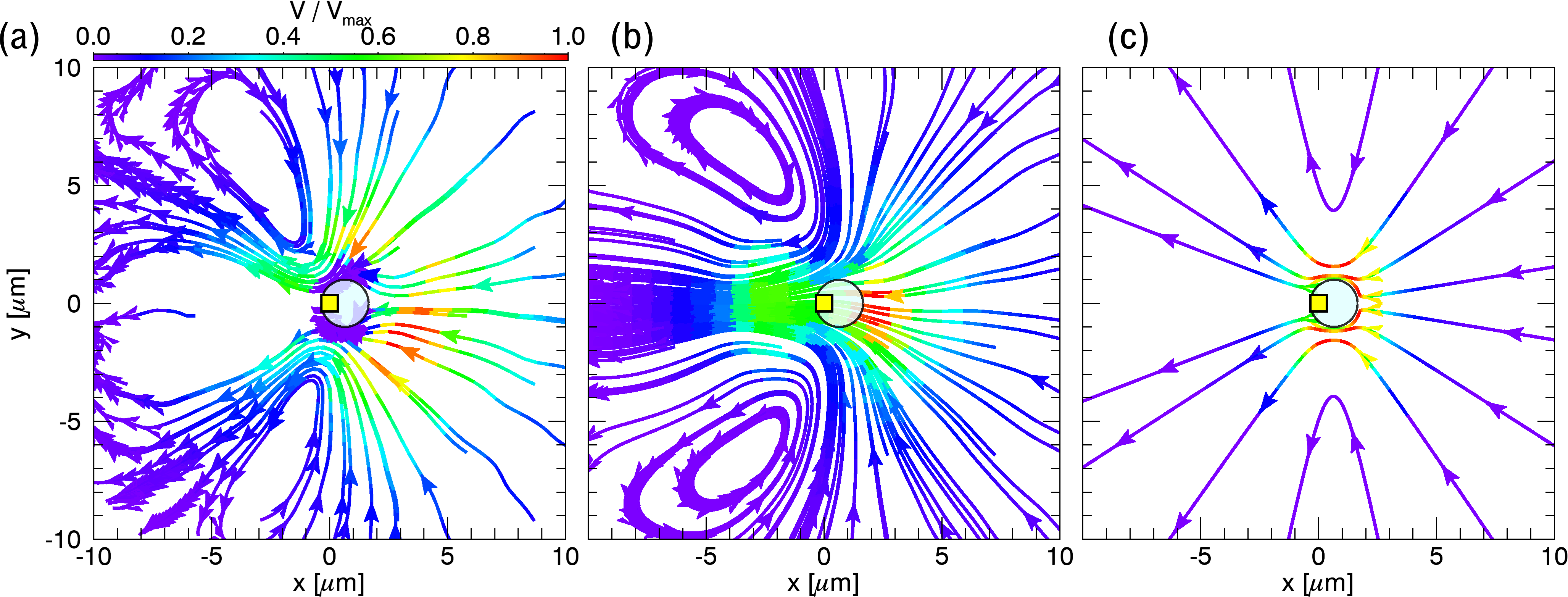
Figure 4: (a) Streamlines of the velocity field, $\mathbf{V}(\mathbf{r})$, of silica tracer particles moving in the vicinity of a stuck swimmer illuminated by a diverging laser beam. (b) Streamlines of the velocity field obtained from simulated trajectories of tracer particles moving under the combined influence of a stuck swimmer’s flow field and thermophoresis in the swimmer’s temperature field. (c) Streamlines of the swimmer’s flow field, $\mathbf{u}(\mathbf{r})$, used in computing (b).

II.3 Other influences on the tracers’ motions

The silica tracer spheres also are acted upon directly by optical forces. We measure this influence by moving the illumination into a region without any hematite cubes and tracking nearby spheres’ motions. These measurements reveal that the spheres are very weakly repelled from the optical axis by the diverging beam’s radiation pressure. The maximum radial drift velocity induced by radiation pressure is much smaller than $1\text{\,}\mathrm{\SIUnitSymbolMicro m}\text{\,}{\mathrm{s}}^{-1}$ and thus no more than a few percent of the thermophoretic or flow-induced drift.

Gravity also influences the tracers’ motions, causing them to drift toward the lower wall of the sample chamber. The resulting sedimentation is slow enough that it may be ignored without qualitatively influencing the observed velocity field.

II.4 Mapping a stationary swimmer’s flow field

Figure 4(a) shows streamlines of the tracer-particle velocity field, $\mathbf{V}(\mathbf{r})$, under steady illumination. The position of the static swimmer is indicated by a circle plotted to scale near the center of the figure, with the cube plotted to scale as a square to the left of the swimmer’s center. The velocity field was computed from 250 independent tracer-particle trajectories with a kernel-density estimate equivalent to Eq. (4). Streamlines were computed with fourth-order Runge-Kutta integration starting from random initial positions. Colors represent the local speed, $V(\mathbf{r})$, and arrows indicating the direction of motion are evenly separated in time. Tracer particles flow predominantly from right to left in Figure 4, with two clear vortexes appearing slightly downstream of the swimmer. No streamlines are plotted directly downstream of the swimmer because no tracer particles ventured into this region. Any tracers originally in that region were expelled to the left before recording began.

Figure 4(b) shows streamlines of the flow field predicted by Faxén’s law, Eq. (17), using as inputs the model for the swimmer’s self-thermophoretic flow field from Eq. (15) and the result for the tracers’ thermophoretic drift from Eq. (19). Qualitative features of the computed velocity field, $\mathbf{V}(\mathbf{r})$, agree very well with the experimental result. The model’s success at reproducing the experimentally observed tracer-particle velocity field justifies its underlying assumptions and approximations.

Incorporating the influence of radiation pressure and sedimentation has little influence on the computed results. Omitting the tracers’ thermophoresis, however, eliminates the paired vortexes downstream of the swimmer. This can be seen in Figure 4(c), which shows streamlines of the swimmer-generated flow field, $\mathbf{u}(\mathbf{r})$, that is calculated with Eq. (15) and was used to compute Figure 4(b). Tracer thermophoresis therefore qualitatively influences our observations; the swimmer’s intrinsic flow field is a continuous stream. The peak flow speed at the swimmer’s position in Figure 4(c) is consistent with the swimmer’s speed when it swims freely, with no adjustable parameters.

III Optical forces and torques

Although the self-thermophoretic mechanism explains the swimmers’ overall propulsion, it does not explain their trajectories’ looping character. Were this the only mechanism influencing the particles’ motion, they would move rapidly to the periphery of the light field, where they would proceed to diffuse. Only if their rotational and translational diffusion directed them back into light would they swim back toward the axis. This process would be slow, however, and the particles would be more likely to diffuse away from the optical axis. Apparently, another mechanism is at work. The nature of this additional influence reveals itself through subtle biases in the thermophoretically-driven motion.

Figure 2(c) establishes, broadly speaking, that the swimmer’s speed is proportional to the local light intensity. This intensity distribution, moreover, is reasonably well described as a Gaussian surface of revolution. In that case, the swimmer’s speed should fall off as a Gaussian with distance from the optical axis. This is consistent with the tracking data for the swimmer’s radial speed, plotted in Figure 5, using the width $\sigma=$7.3\text{\,}\mathrm{\SIUnitSymbolMicro m}$$ obtained from imaging photometry of the beam.

These data, however, also show a more subtle feature: the radial speed is slightly but systematically higher when the particle is moving radially outward, $\mathbf{v}(t)\cdot\hat{r}>0$, than when it moves radially inward, $\mathbf{v}(t)\cdot\hat{r}<0$. The radial speeds plotted in Figure 5(a) are computed separately for the inward- and outward-moving trajectory segments. For these measurements, the swimmer is defined to be located at the position of its cube, $\mathbf{r}_{c}$. This avoids systematic offsets due to variations in $I(\mathbf{r})$ across the sphere’s diameter. The difference between inward and outward radial speeds, is plotted in Figure 5.

Figure 5: (a) Radial component of the swimmer’s velocity, $v_{r}(r)$, as it moves either inward toward the center of the intensity distribution (blue symbols) or outward (red). The dashed curve is a fit to a Gaussian corresponding to the measured intensity distribution of the illumination. Speeds are normalized by the peak speed, $v_{0}$, of this fit. (b) Difference, $\Delta v_{r}(r)$, between outward and inward radial speeds, together with a fit to Eq. (21).

The difference in radial speeds is consistent with the action of a small outward-directed force. The dashed curve is a comparison with expectations for the in-plane component of radiation pressure,

$$\Delta v_{r}(r)=\alpha_{r}I(\mathbf{r})\frac{r}{\sqrt{r^{2}+L^{2}}},$$ (21)

where the constant $\alpha_{r}$ sets the scale for the light-matter coupling. We already have determined that the influence of radiation pressure on the TPM sphere is negligibly weak. Any influence of radiation pressure therefore must result from absorption of light by the hematite cube, which also is responsible for the swimmer’s self-thermophoresis. The dashed curve in Figure 5(b) is obtained with $\alpha_{r}=$3\pm 2.\text{\,}{\mathrm{\SIUnitSymbolMicro m}}^{3}\text{\,}{\mathrm{s}}^{-1}\text{\,}{\mathrm{mW}}^{-1}$$ and no other adjustable parameters. This is consistent with the expected in-plane component of the radiation pressure that would arise from complete absorption of the light by a cube $300\text{\,}\mathrm{nm}$ on a side.

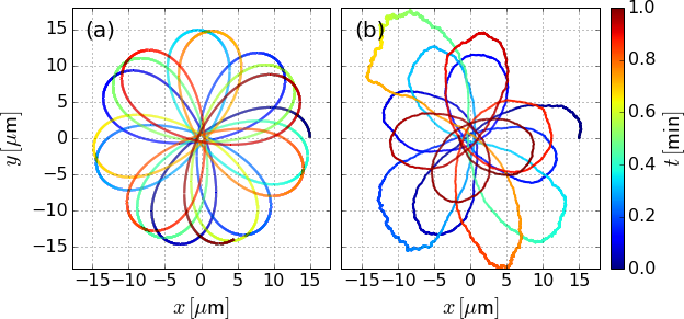
Figure 6: Computed trajectory for a swimmer moving under the combined influence of self-thermophoresis and optical torque. (a) Trajectory traced out in the absence of thermal noise. (b) Equivalent trajectory including both translational and rotational diffusion.

The mean radial velocity of the swimmer thus provides evidence for a small contribution from radiation pressure acting on the cube that supplements the hydrodynamic force acting on the sphere. Although radiation pressure is weak, it strongly influences the swimmer’s motion by exerting a torque on the sphere. The torque arises because radiation pressure acts on the cube rather than on the sphere, and acts in the radial direction, $\hat{r}$, which need not be aligned with the swimmer’s orientation, $\hat{n}$. Radiation pressure therefore causes rotation about the axis of the sphere with an angular velocity

$$\boldsymbol{\omega}(\mathbf{r})=\mu_{\theta}\alpha_{r}\frac{a}{\sqrt{2}}I(\mathbf{r})\,\frac{r}{\sqrt{r^{2}+L^{2}}}\,\hat{r}\times\hat{n},$$ (22)

where $\mu_{\theta}$ is the swimmer’s rotational mobility.

IV Trochoidal motion

If, for the sake of simplicity, we consider optical torque but neglect the contribution of radiation pressure to the swimmer’s velocity, and furthermore treat the sphere as being small ($a\ll\sigma$), we then may model the velocity as being proportional to the local intensity

$$v(r)\approx\frac{v_{0}}{I_{0}}\,I(r)$$ (23)

with a characteristic speed for the present system $v_{0}=$40\pm 2.\text{\,}\mathrm{\SIUnitSymbolMicro m}\text{\,}{\mathrm{s}}^{-1}$$. The particle also diffuses under the influence of random thermal forces. The set of coupled Langevin equations describing the particle’s in-plane are

$$\dot{x}(t) =v(r(t))\cos(\phi(t))+\zeta(t)\quad\text{and}$$ (24a)

$$\dot{y}(t) =v(r(t))\sin(\phi(t))+\zeta(t),$$ (24b)

where $$\phi(t)=\tan^{-1}(y(t)/x(t)) \hat{x} \zeta(t)$$ is the swimmer’s orientation relative to , and is a normally distributed random variable that models thermal noise. The swimmer’s orientation evolves according to Eq. (22), and also is influenced by thermal fluctuations,

$$\dot{\phi}(t)=\frac{x(t)\dot{y}(t)-y(t)\dot{x}(t)}{d\sqrt{r^{2}(t)+L^{2}}}+\sqrt{\frac{3}{4a^{2}}}\,\zeta(t),$$ (24c)

where $d$ sets the scale of rotations relative to translations.

Figure 6(a) shows a typical trajectory obtained by Euler-Maruyama integration of Eq. (24) in the absence of noise ($\zeta(t)=0$) for parameters chosen to mimic the experimental conditions in Figure 2(b). These deterministic equations admit periodic solutions,

$$x(t+T) =x(t)$$ (25a)

$$y(t+T) =y(t)$$ (25b)

$$\phi(t+T) =\phi(t)+2m\pi,$$ (25c)

where $m$ is an integer. Traces such as the example in Figure 6(a) at least qualitatively resemble rosette curves.

One special case of a deterministic rosette trajectory is the circular path,

$$x_{0}(t) =\frac{v_{0}}{\omega}\sin(\omega t)$$ (26a)

$$y_{0}(t) =-\frac{v_{0}}{\omega}\cos(\omega t),$$ (26b)

which is generated by having the swimmer rotate once per orbit:

$$\phi_{0}(t)=\omega t.$$ (26c)

This trajectory has a radius $$R$$ that satisfies

$$R^{2}=\frac{1}{2}\,d^{2}\,\left(1+\sqrt{1+4\frac{L^{2}}{d^{2}}}\right)$$ (26d)

and a corresponding angular frequency

$$\omega=\frac{2\pi}{T}=\frac{v_{0}}{R}\,\exp\left(-\frac{R^{2}}{2\sigma^{2}}\right).$$ (26e)

Perturbing this solution,

$$\phi(t)=\phi_{0}(t)+\epsilon\sin(b\omega t),$$ (27a)

yields the hypotrochoidal solutions

$$x(t) =x_{0}(t)-\frac{\epsilon v_{0}}{2\omega}\left[\frac{\sin\left((1-b)\omega t\right)}{1-b}-\frac{\sin\left((1+b)\omega t\right)}{1+b}\right]$$ (27b)

$$y(t) =y_{0}(t)+\frac{\epsilon v_{0}}{2\omega}\left[\frac{\cos\left((1-b)\omega t\right)}{1-b}-\frac{\cos\left((1+b)\omega t\right)}{1+b}\right],$$ (27c)

up to corrections at $\mathcal{O}\left\{\epsilon^{2}\right\}$. These solutions self-consistently satisfy Eq. (24) up to $\mathcal{O}\left\{\epsilon^{2}\right\}$ for the particular choice $b=\sqrt{2}$, and closely resemble the numerical solution in Figure 6(a) for appropriate choices of the perturbation amplitude, $\epsilon$.

Other solutions include non-repeating trajectories in which the particle swims radially outward, never to return. We designate these as open or escape trajectories.

Figure 6(b) shows a typical numerical solution of the trochoidal trajectory from Figure 6(a) including the influence of random thermal forces and torques at room temperature. This simulation was performed with $d=$3.57\text{\,}\mathrm{\SIUnitSymbolMicro m}$$, which suggests that that the rotation rate due to optical torque is only a third the rate of rotational diffusion. Optical torque, however, acts in a sense governed by the swimmer’s orientation, and so imposes a coherent structure on the trajectory. Small translational displacements roughen the curve but otherwise have little effect on its extent or orbital frequency. Random rotations, however, transfer the swimmer from one trochoidal orbit to another. Because an orbit’s radial extent is strongly influenced by the swimmer’s orientation near the origin, small diffusional rotations can have a disproportionate influence on the scale of the pattern that the swimmer traces out. This process accounts for the ability of the trap to capture a swimmer, and provides a mechanism for the swimmer ultimately to escape.

V Conclusions

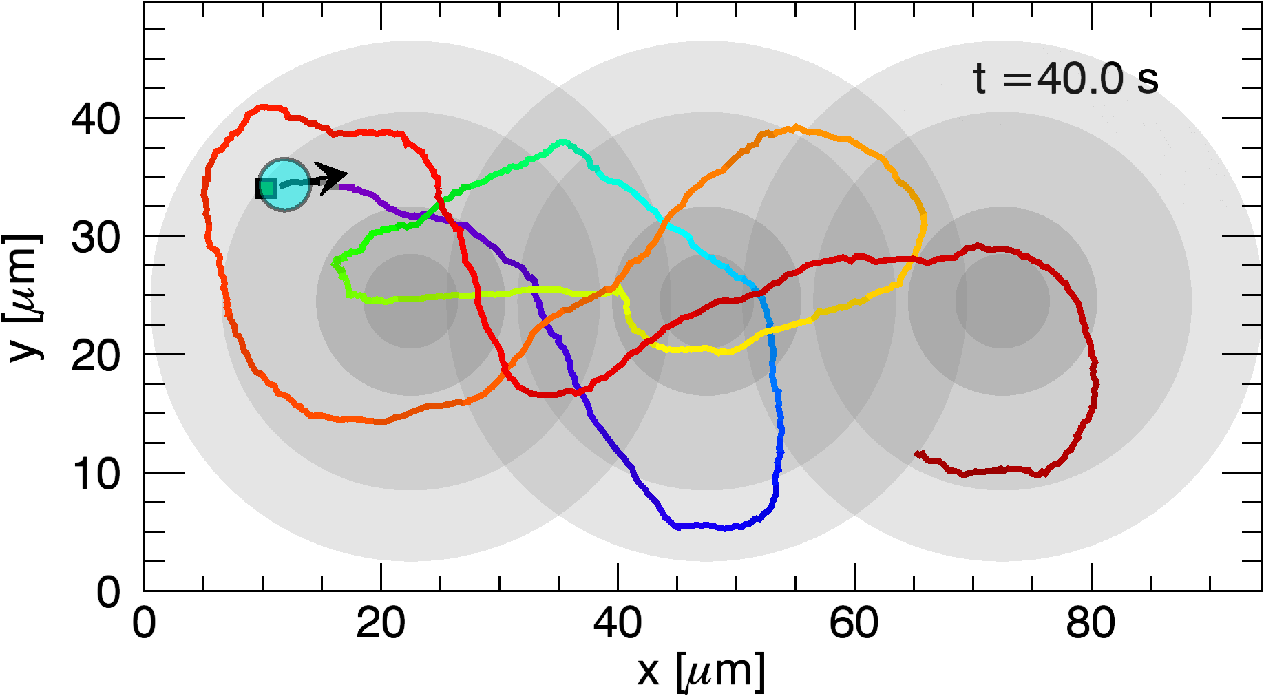
Figure 7: Measured trajectory of a swimmer moving under the influence of three defocused point traps over the course of $40\text{\,}\mathrm{s}$. Gray regions are contours of the light intensity. The swimmer is drawn to scale at the outset of its trajectory.

Composite colloidal particles consisting of optically absorbing hematite cubes embedded in transparent colloidal spheres act as self-thermophoretic swimmers. These particles move through water when illuminated without requiring chemical fuel, employing a propulsion mechanism that is captured by a low-level stokeslet formulation. When activated by a nonuniform light field, these swimmers also experience optically-induced torques that tend to orient their motions. In the particular case of diverging illumination, this causes the swimmers to become confined to looping paths that we identify with rosette curves in general and trochoids in particular. Random thermal forces and torques perturb these patterns into paths that we call stochastic trochoidal trajectories. The observation of such trajectories provides experimental support for the proposed propulsion mechanism.

Optically-activated self-thermophoretic swimmers constitute a rich model system for studying active matter. While the present study focuses on the behavior of a single particle moving in a comparatively simple light field, prospects are bright for studying behavior in more sophisticated systems. Figure 7, for example, shows the experimentally measured trajectory of a single particle moving under the influence of an array of three uniformly bright defocused optical tweezers, each of which resembles the single tweezer used for the foregoing studies. The particle repeatedly loops through the entire pattern.

Multiple swimmers moving through the same light field are driven both by their interaction with the light and also by their long-ranged hydrodynamic interactions. The strength and direction of these interactions depends on the swimmers’ positions in the light field and on their relative orientations. Introducing position-dependent coupling in nonuniform light fields creates an opportunity to study the influence of dynamic heterogeneity on collective behavior in active matter.

References

- Golestanian et al. (2005) R. Golestanian, T. B. Liverpool and A. Ajdari, Phys. Rev. Lett., 2005, 94, 220801.
- Marchetti et al. (2013) M. C. Marchetti, J. F. Joanny, S. Ramaswamy, T. B. Liverpool, J. Prost, M. Rao and R. A. Simha, Rev. Mod. Phys., 2013, 85, 1143.
- Walther and Müller (2008) A. Walther and A. H. E. Müller, Soft Matter, 2008, 4, 663–668.
- Paxton et al. (2004) W. F. Paxton, K. C. Kistler, C. C. Olmeda, A. Sen, S. K. St. Angelo, Y. Cao, T. E. Mallouk, P. E. Lammert and V. H. Crespi, J. Am. Chem. Soc., 2004, 126, 13424–13431.
- Jiang et al. (2010) H.-R. Jiang, N. Yoshinaga and M. Sano, Phys. Rev. Lett., 2010, 105, 268302.
- Volpe et al. (2011) G. Volpe, I. Buttinoni, D. Vogt, H.-J. Kümmerer and C. Bechinger, Soft Matter, 2011, 7, 8810–8815.
- Buttinoni et al. (2012) I. Buttinoni, G. Volpe, F. Kümmel, G. Volpe and C. Bechinger, J. Phys.: Condens. Matter, 2012, 24, 284129.
- Buttinoni et al. (2013) I. Buttinoni, J. Bialké, F. Kümmel, H. Löwen, C. Bechinger and T. Speck, Phys. Rev. Lett., 2013, 110, 238301.
- Qian et al. (2013) B. Qian, D. Montiel, A. Bregulla, F. Cichos and H. Yang, Chem. Sci., 2013, 4, 1420–1429.
- Bickel et al. (2014) T. Bickel, G. Zecua and A. Würger, Phys. Rev. E, 2014, 89, 050303(R).
- Sacanna et al. (2012) S. Sacanna, L. Rossi and D. J. Pine, J. Am. Chem. Soc., 2012, 134, 6112–6115.
- Abrikosov et al. (2013) A. I. Abrikosov, S. Sacanna, A. P. Philipse and P. Linse, Superlattices Microstructures, 2013, 9, 8904–8913.
- Palacci et al. (2013) J. Palacci, S. Sacanna, A. P. Steinberg, D. J. Pine and P. M. Chaikin, Science, 2013, 339, 936–940.
- Palacci et al. (2014) J. Palacci, S. Sacanna, S.-H. Kim, G.-R. Yi, D. J. Pine and P. M. Chaikin, Phil. Trans. Roy. Soc. A, 2014, 372, 20130372.
- Weinert and Braun (2008) F. W. Weinert and D. Braun, Phys. Rev. Lett., 2008, 101, 168301.
- Yang and Ripoll (2013) M. Yang and M. Ripoll, Superlattices Microstructures, 2013, 9, 4661–4671.
- Crocker and Grier (1996) J. C. Crocker and D. G. Grier, J. Colloid Interface Sci., 1996, 179, 298–310.
- Krishnatreya and Grier (2014) B. J. Krishnatreya and D. G. Grier, Opt. Express, 2014, 22, 12773–12778.
- Silverman (1992) B. W. Silverman, Density Estimation for Statistics and Data Analysis, Chapman & Hall, New York, 1992.
- Iacopini et al. (2006) S. Iacopini, R. Rusconi and R. Piazza, Euro. Phys. J. E, 2006, 19, 59–67.
- Fayolle et al. (2008) S. Fayolle, T. Bickel and A. Würger, Phys. Rev. E, 2008, 77, 041404.
- Pozrikidis (1992) C. Pozrikidis, Boundary Integral and Singularity Methods for Linearized Viscous Flow, Cambridge University Press, New York, 1992.
- Blake (1971) J. R. Blake, Proc. Cambridge Phil. Soc., 1971, 70, 303–310.
- Liron and Mochon (1976) N. Liron and S. Mochon, J. Eng. Math., 1976, 10, 287.
- Dufresne et al. (2001) E. R. Dufresne, D. Altman and D. G. Grier, Europhys. Lett., 2001, 53, 264–270.
- Spagnolie and Lauga (2012) S. E. Spagnolie and E. Lauga, J. Fluid Mech., 2012, 700, 105–147.