Renormalization Group Approach to Stability of Two-dimensional Interacting Type-II Dirac Fermions

Abstract

The type-II Weyl/Dirac fermions are a generalization of conventional or type-I Weyl/Dirac fermions, whose conic spectrum is tilted such that the Fermi surface becomes lines in two dimensions, and surface in three dimensions rather than discrete points of the conventional Weyl/Dirac fermions. The mass-independent renormalization group calculations show that the tilting parameter decreases monotonically with respect to the length scale, which leads to a transition from two dimensional type-II Weyl/Dirac fermions to the type-I ones. Because of the non-trivial Fermi surface, a photon gains a finite mass partially via the chiral anomaly, leading to the strong screening effect of the Weyl/Dirac fermions. Consequently, anisotropic type-II Dirac semimetals become stable against the Coulomb interaction. This work provides deep insight into the interplay between the geometry of Fermi surface and the Coulomb interaction.

I Introduction

Three-dimensional (3D) Weyl semimetals are topological states of quantum matter and can be regarded as 3D analogues of graphene Wan et al. (2011); Weng et al. (2016). Their conduction and valence bands with linear dispersion touch each other at a finite number of points, called the Weyl nodes, in the 3D Brillouin zone. These Weyl nodes can be viewed as magnetic monopoles in momentum space Xiao et al. (2010); Volovik (2003), which lead to various novel electromagnetic responses such as the chiral anomaly Nielsen and Ninomiya (1983); Aji (2012); Wang and Zhang (2013); Liu et al. (2013); Goswami and Tewari (2013); Parameswaran et al. (2014), chiral magnetic effect Fukushima et al. (2008); Grushin (2012); Zyuzin and Burkov (2012); Zhou et al. (2013); Vazifeh and Franz (2013); Chang and Yang (2015); Ma and Pesin (2015); Zhong et al. (2016), and exotic magnetoresistance Son and Spivak (2013); Gorbar et al. (2014); Burkov (2014); Lu et al. (2015). Very recently, a new kind of Weyl/Dirac semimetals with the tilted conic spectrum, named type-II Weyl/Dirac semimetals, have been predicted in a series of materials Soluyanov et al. (2015); Sun et al. (2015); Koepernik et al. (2016); Autès et al. (2016), in which the Fermi surface crossing the Weyl nodes is lines in two dimensions Goerbig et al. (2008) and surface in three dimensions Soluyanov et al. (2015) with a finite density of states (DOS). Meanwhile, many experiments have made great efforts to characterize type-II Weyl/Dirac semimetals by angle-resolved photoemission spectroscopy Huang et al. (2016); Xu et al. (2016); Wang et al. (2016). This nontrivial Fermi surface could lead to an exotic magnetic-optical response Yu et al. (2016); Tchoumakov et al. (2016); Udagawa and Bergholtz (2016) and unconventional magnetic breakdown O’Brien et al. (2016).

Coulomb interaction plays a crucial role in understanding the properties and stability of the Fermi surface in both two-dimensional (2D) Kotov et al. (2012) and 3D Dirac/Weyl semimetals Abrikosov and Beneslavskii (1971); Zhou et al. (2015); Hofmann and Das Sarma (2015). For type-I 2D Dirac semimetals, the vanishing DOS at Fermi points does not screen the Coulomb interaction sufficiently Kotov et al. (2012). The renormalization group (RG) Shankar (1994); Polchinski (1992) calculations show that the Coulomb interaction renormalizes the effective velocity and makes it diverge logarithmically González et al. (1999); Son (2007). One solution to this unphysical divergence is to take into account the relativistic effect in the full quantum electrodynamics level Isobe and Nagaosa (2016) such that the velocity of fermions is renormalized up to the speed of light Isobe and Nagaosa (2012). In this work, we study 2D type-II Dirac semimetals that possess an extended Fermi surface (two lines) and finite DOS even when the Fermi surface crosses the Weyl nodes. It is natural to wonder how this nontrivial geometry of Fermi lines interplays with both the Coulomb interaction and the finite DOS.

It has been shown that under the unscreened Coulomb interaction, the tilting parameter is a monotonic decreasing function of length scale such that the 2D type-II Dirac fermions transit to the type-I ones. Because of the non-trivial Fermi surface, a photon gains a finite mass partially via the chiral anomaly, giving rise to a strong screening effect. Consequently, anisotropic type-II Dirac fermions become stable against the Coulomb interaction. In addition, the logarithmic divergence of Fermi velocity is substantially suppressed. This work sheds new light on the interaction effect of 2D type-II Dirac semimetals.

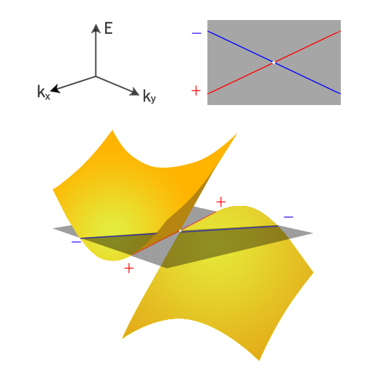
Figure 1: The energy bands and Fermi surface of 2D type-II Dirac fermions. The dark plane is the iso-energy surface crossing the Weyl node located by the white intersection point. The red and blue lines labeled by $\pm$ denote the Fermi lines.

II model for 2d tilted Dirac fermions

In the present work, we shall focus on the 2D tilted Dirac fermions that respect the inversion symmetry or time reversal symmetry to prevent the band-gap opening. Actually, the quasi-2D conducting organic compound $\alpha-\left(\mathrm{BEDT-TTF}\right)_{2}\mathrm{I}_{3}$ supports these tilted Dirac fermions Bender et al. (1984); Katayama et al. (2006); Hirata et al. (2016). We start with the following Hamiltonian for 2D type-II Dirac fermions, in which the conic spectrum is tilted along the $x$-axis (we set $\hbar=1$) Goerbig et al. (2008),

$$H_{0}=v_{x}p_{x}\sigma^{1}+v_{y}p_{y}\sigma^{2}+wv_{x}p_{x},$$ (1)

where $w$ refers to a tilting parameter for type-II Dirac fermions with $|w|>1$ and for type-I ones otherwise. $v_{x}$ and $v_{y}$ denote for the velocity along the $x$-axis and $y$-axis, respectively. For simplicity, we denote the ratio of two velocities by $\eta=v_{x}/v_{y}$. $\sigma^{i}$ with $i=1,2$ are the Pauli matrices. The energy dispersions of Eq. (1) are of the form

$$E_{\pm}=wv_{x}p_{x}\pm\sqrt{v_{x}^{2}p_{x}^{2}+v_{y}^{2}p_{y}^{2}}.$$ (2)

There are two Fermi lines at $E_{\pm}=0$ in the $p_{x}-p_{y}$ plane, described by $p_{y}=\pm\tilde{w}\eta p_{x}$ with $\tilde{w}=\sqrt{w^{2}-1}$. $\pm$ refers to the sign of slope of each Fermi line as shown in Fig. 1. Note that the energy dispersion in Eq. $\left(\ref{Edisp}\right)$ is only valid for a finite region near each Weyl node, we thus introduce a momentum cut-off $\Lambda$ along the $p_{x}$-axis. Since the Fermi surface is not point-like, one needs to expand the Hamiltonian in Eq. (1) around the Fermi lines to capture the low-energy properties Polchinski (1992); Shankar (1994). Namely, we decompose the momentum into two parts: the momentum parallel to the Fermi lines $k_{F}$ and the momentum perpendicular to the Fermi lines $\tilde{p}$,

$$k_{F}^{\pm} = (p_{\parallel},\pm\tilde{w}\eta p_{\parallel}),$$

$$\tilde{p}^{\pm} = (\pm\tilde{w}\eta p_{\perp},-p_{\perp})$$ (3)

with $J=1+\tilde{w}^{2}\eta^{2}$ being the corresponding Jacobian. $p_{\|}$ and $p_{\bot}$ are the $x$-component of $k_{F}^{\pm}$ and $y$-component of $\tilde{p}^{\pm}$, respectively, where the subscript $\|$ $\left(\bot\right)$ denotes for momentum parallel (perpendicular) to the Fermi lines. In terms of $k_{F}^{\pm}$ and $\tilde{p}^{\pm}$, the Hamiltonian in Eq. (1) can be recast as

$$H_{0}=H_{k_{F}^{\pm}}+H_{\tilde{p}^{\pm}},$$ (4)

where $H_{k_{F}^{\pm}}$ and $H_{\tilde{p}^{\pm}}$ only depend on $p_{\parallel}$ and $p_{\perp}$, respectively. The corresponding Lagrangian for electrons can be directly obtained from $H_{k_{F}^{\pm}}$ and $H_{\tilde{p}^{\pm}}$,

$$\mathcal{L}_{e} =\Sigma_{s=\pm}\Psi_{s}^{\dagger}\left[p_{0}-\left(H_{k_{F}^{s}}+H_{\tilde{p}^{s}}\right)p_{\perp}\right]\Psi_{s}$$

$$=\Psi_{+}^{\dagger}(p_{\bot})\left[p_{0}-\left(w\tilde{w}\eta^{2}+\tilde{w}\eta^{2}\sigma^{1}-\sigma^{2}\right)v_{y}p_{\perp}\right]\Psi_{+}(p_{\bot})$$

$$+\Psi_{-}^{\dagger}\left(-p_{\bot}\right)\left(-i\sigma^{2}\right)\left[p_{0}-\left(w\tilde{w}\eta^{2}-\tilde{w}\eta^{2}\sigma^{1}+\sigma^{2}\right)v_{y}p_{\perp}\right]$$

$$\times\left(i\sigma^{2}\right)\Psi_{-}\left(-p_{\bot}\right),$$ (5)

where $\Psi_{s}$ with $s=\pm$ denote for fermions on two different Fermi lines and satisfy the relation $\Psi_{\pm}^{\dagger}H_{k_{F}^{\pm}}\Psi_{\pm}=0$ due to zero Fermi energy. After introducing a new spinor

$$\bar{\Psi}\left(p_{\bot}\right)=\left(\Psi_{-}^{\dagger}\left(-p_{\bot}\right)(-i\sigma^{2}),\Psi_{+}^{\dagger}\right)\gamma^{0},$$ (6)

the action can be recast as

$$S_{0} = \int\frac{dp_{0}dp_{\parallel}dp_{\perp}}{\left(2\pi\right)^{3}}J(\mathcal{L}_{e}+\mathcal{L}_{\gamma}+\mathcal{L}_{I}),$$ (7)

where $\mathcal{L}_{e}$, $\mathcal{L}_{\gamma}$ and $\mathcal{L}_{I}$ denote the Lagrangians for electrons, photons and the interaction between electrons and photons, respectively. Their specific expressions are given as

$$\mathcal{L}_{e} = \bar{\Psi}\left[p_{0}\gamma^{0}-\left(w\tilde{w}\eta^{2}\gamma^{0}+\tilde{w}\eta^{2}\gamma^{1}-\gamma^{2}\right)v_{y}p_{\perp}\right]\Psi,$$

$$\mathcal{L}_{\gamma} = \int\frac{dp_{z}}{4\pi}\phi\left[J\left(p_{\parallel}^{2}+p_{\perp}^{2}\right)+p_{z}^{2}\right]\phi,$$

$$\mathcal{L}_{I} = \bar{\Psi}\left(-e\gamma^{0}\phi\right)\Psi,$$ (8)

where $\gamma^{\mu}$ with $\mu=0,1,2$ are the $4\times 4$ Dirac gamma matrices including the extra two degrees of freedom for the two Fermi lines. $\phi$ refers to the field of photons. By use of the Hubbard-Stratonovich transformation, one obtains both $\mathcal{L}_{\gamma}$ and $\mathcal{L}_{I}$ from the Coulomb interaction,

$$(\bar{\Psi}\gamma^{0}\Psi)(-p)V(q)(\bar{\Psi}\gamma^{0}\Psi)(p),$$

which describes both the inter- and the intra-Fermi line interactions and satisfies the restriction given by the Fermi surface at tree level. $V(q)=e^{2}/\sqrt{q_{x}^{2}+q_{y}^{2}}$ is the Fourier transformation of a bare 2D Coulomb potential. Additionally, $\mathcal{L}_{\gamma}$ is actually the non-relativistic limit of the action $-\frac{1}{4}\int\frac{d^{4}p}{(2\pi)^{4}}F^{\mu\nu}F_{\mu\nu}$ in the Feynman-’t Hooft gauge with $F_{\mu\nu}$ being the electromagnetic field strength tensor. $\int\frac{dp_{z}}{2\pi}$ in $\mathcal{L}_{\gamma}$ comes from Son (2007)

$$\frac{1}{2\sqrt{p_{x}^{2}+p_{y}^{2}}}=\int\frac{dp_{z}}{2\pi}\frac{1}{p_{x}^{2}+p_{y}^{2}+p_{z}^{2}},$$ (9)

where we have set the speed of light $c=1$ for simplicity. It should be noted that when $\tilde{w}=0$, the Fermi surface at $E_{\pm}=0$ becomes a straight line and the Lagrangian for electrons reduces to be

$$\mathcal{L}_{e}=\bar{\Psi}\left(p_{0}\gamma^{0}+\gamma^{2}v_{y}p_{\perp}\right)\Psi,$$ (10)

which is nothing but the famous Schwinger model for the $\left(1+1\right)$D massless Dirac fermions Schwinger (1962). Under this circumstance, the photon gains a finite mass due to the chiral anomaly Adler (1969); Bell and Jackiw (1969); Roskies and Schaposnik (1981). A finite photon mass usually leads to a strong screening effect in the long-range Coulomb interaction. In fact, the screening effect shall play a critical role in suppressing the logarithmic divergence of Fermi velocity and stabilizing the 2D anisotropic type-II Dirac fermions.

III The screening effect from analysis of random phase approximation

The finite DOS and the extended Fermi surface in the type-II Weyl/Dirac semimetals remind us of the role of the screening effect. By calculating the vacuum polarization diagram in Fig. (2b) (the detailed derivations are given in Appendix ), one finds

$$\Pi^{00}\left(p_{0},\vec{p}\right) =-i\int J\mathrm{tr}\left(\Gamma_{0}G_{e0}\Gamma_{0}G_{e0}\right)$$

$$=\frac{4e^{2}}{\pi}\frac{\Lambda^{2}\mathcal{C}^{-1}\left(1+\tilde{w}^{2}\eta^{2}\right)p_{\perp}^{2}}{(p_{0}+w^{2}\tilde{w}^{2}\eta^{4}p_{\perp})^{2}-\mathcal{C}^{-2}p_{\perp}^{2}},$$ (11)

where $\Gamma_{0}$ and $G_{e0}$ are the vertex and electron’s propagator, respectively, and $\mathcal{C}=1/\sqrt{v_{y}^{2}\left(\tilde{w}^{2}\eta^{4}+1\right)}$. Several remarks on $\Pi^{00}\left(p_{0},\vec{p}\right)$ are in order here. First,

$$\Pi^{00}(0,\vec{p})=\frac{4e^{2}}{\pi}\frac{\Lambda^{2}\mathcal{C}^{-1}\left(1+\tilde{w}^{2}\eta^{2}\right)}{w^{4}\tilde{w}^{4}\eta^{8}-\mathcal{C}^{-2}}$$ (12)

is a momentum independent constant and relates to the quadratic potential for photon mass. Second, a negative quadratic potential usually indicates an instability of the system Srednicki (2007). In addition, in the limit of $\tilde{w}\rightarrow 0$, one finds

$$\lim_{\tilde{w}\rightarrow 0}\frac{\Pi^{00}(p_{0},\vec{p})}{2\Lambda^{2}\left(\tilde{w}^{2}\eta^{2}+1\right)\mathcal{C}}=\frac{2e^{2}}{\pi v_{y}}\frac{v_{y}^{2}p_{\bot}^{2}}{p_{0}^{2}-v_{y}^{2}p_{\bot}^{2}},$$ (13)

which is the same as the one of the Schwinger model that is effectively induced by (1+1)D chiral anomaly Schwinger (1962); Roskies and Schaposnik (1981). In the remainder of this paper, we shall focus on the case with negative $\Pi^{00}(0,\vec{p})$ .

The extended Fermi surface makes the random phase approximation (RPA) reasonable Shankar (1994). Following the standard procedure, one finds the effective Coulomb potential within the RPA:

$$V_{\mathrm{eff}}(\vec{p})=V\left(\vec{p}\right)/\epsilon\left(\vec{p}\right),$$ (14)

where the static dielectric function $\epsilon\left(\vec{p}\right)$ is given as

$$\epsilon(\vec{p})=1-V(\vec{p})\text{$\Pi$}^{00}(0,\vec{p}).$$ (15)

According to $\epsilon(\vec{p})$, for the long-range interaction with small momentum $p$, the magnitude of dielectric function is much larger than 1, which reduces the strength of the Coulomb interaction. On the other hand, for the short-range interaction with large momentum, the magnitude of the dielectric function is almost 1, so the Coulomb interaction is almost not modified. That is, the long-range interaction is screened due to the extended Fermi surface, however the short-range one is not screened. Since the renormalized effect upon the one-body operator induced by the short-range interaction can be absorbed by the chemical potential Shankar (1994), the analysis above implies both the Fermi velocities $v_{x}$ and $v_{y}$, and the tilting parameter $w$ are intact under the screened Coulomb interaction.

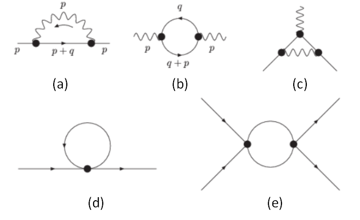
Figure 2: Relevant Feynman diagrams: (a), (b) and (c) are the diagrams without decoupling effect, whereas (d) and (e) are the corresponding diagrams with decoupling effect.

IV renormalization group analysis

Now we turn to consider the running effect of coupling constants under the influence of the Coulomb interaction. We employ the dimensional regularization and the modified minimal subtraction ($\overline{MS}$) scheme Srednicki (2007) to derive the corresponding RG equations, with the help of Feynman’s rules obtained from the Lagrangian in Eq. (8). The bare action is given as

$$\mathcal{L}_{\text{bare}} = \bar{\Psi}[(Z_{\Psi}p_{0}-Z_{w}w\tilde{w}\eta^{2}v_{y}p_{\perp}-Z_{e}e\phi)\gamma^{0}$$ (16)

$$-Z_{\tilde{w}\eta^{2}v_{y}}\tilde{w}\eta^{2}v_{y}p_{\perp}\gamma^{1}+Z_{v_{y}}v_{y}p_{\perp}\gamma^{2}]\Psi,$$

where $Z$’s are the renormalization coefficients. Because of the U(1) symmetry, the Ward identity is valid, which implies the relation: $Z_{\text{$\Psi$\ }}=Z_{e}.$ The vacuum polarization diagram does not diverge in Eq. (11), so no divergence is needed to be canceled by $Z_{\phi}$. Thus, its value is $Z_{\phi}=1.$ The relation between the bare coupling constant $e_{0}$ and the coupling constant $e$ is given as

$$e_{0}=Z_{\Psi}^{-1}Z_{e}Z_{\phi}^{-1}e,$$ (17)

which leads to $e_{0}=e$. It means that the coupling constant $e$ would not be renormalized. Then we use the dimensional regularization to deal with the divergent one-loop self-energy in Fig. (2a) (see Appendix A)

$$-i\Sigma\left(p\right)=\int J\text{ }\Gamma_{0}G_{e0}\Gamma_{0}G_{\gamma 0},$$ (18)

where the photon’s propagator $G_{\gamma 0}$ can be read directly from the Lagrangian in Eq. $\left(\ref{Lagepi}\right)$. Note that we temporarily ignore the screening effect stemming from finite DOS in the photon’s propagator. There exists a natural momentum cut-off $\Lambda$ along the $p_{x}$-direction, which characterizes the length of Fermi lines and is irrelevant to the energy scale. Since the procedure of renormalization is implemented upon the momentum perpendicular to Fermi surface rather than the parallel one, $\Lambda$ plays no role in the renormalization.

By using the $\overline{MS}$ scheme, one can obtain the following RG equations for the effective velocities and the tilting parameter. The bare action is given as

$$\mathcal{L} = \bar{\Psi}[(Z_{\Psi}p_{0}-Z_{w}w\tilde{w}\eta^{2}v_{y}p_{\perp})\gamma^{0}-$$ (19)

$$Z_{\tilde{w}\eta^{2}v_{y}}\tilde{w}\eta^{2}v_{y}p_{\perp}\gamma^{1}+Z_{v_{y}}v_{y}p_{\perp}\gamma^{2}]\Psi.$$

By comparing the bare action with the renormalized one, one gets a set of equations

$$\Psi_{0} = Z_{\Psi}^{1/2}\Psi,$$ (20)

$$v_{y0} = Z_{v_{y}}Z_{\Psi}^{-1}v_{y},$$ (21)

$$\left(\tilde{w}\eta^{2}v_{y}\right)_{0} = Z_{\tilde{w}\eta^{2}v_{y}}Z_{\Psi}^{-1}\left(\tilde{w}\eta^{2}v_{y}\right),$$ (22)

$$w_{0} = Z_{w}Z_{\tilde{w}\eta^{2}v_{y}}^{-1}Z_{\Psi}^{-1}w,$$ (23)

where $Z_{\Psi}$, $Z_{w}$, $Z_{\tilde{w}\eta^{2}v_{y}}$ and $Z_{v_{y}}$ are given as

$$Z_{\Psi}=Z_{w} = 1,$$ (24)

$$Z_{\tilde{w}\eta^{2}v_{y}}=Z_{v_{y}} = 1-\frac{e^{2}}{8\pi^{2}\epsilon}F.$$ (25)

After some standard derivations, one gets the corresponding RG equations

$$\frac{d\ln v_{y}}{d\ln\kappa}=\frac{d\ln(\tilde{w}\eta^{2}v_{y})}{d\ln\kappa}=-\frac{d\ln w}{d\ln\kappa}=\mathcal{B},$$ (26)

where $\kappa$ is the renormalization scale, i.e., the larger $\kappa$, the smaller the energy scale. The function $\mathcal{B}\left(w,\ v_{x},\ v_{y}\right)$ is defined by

$$\mathcal{B}\left(w,v_{x},v_{y}\right) =\frac{e^{2}}{4\pi^{2}} \frac{\sqrt{1+\tilde{w}^{2}\eta^{2}}}{\sqrt{v_{y}^{2}\left(1+\tilde{w}^{2}\eta^{4}\right)}}.$$ (27)

From these RG equations in Eq. $\left(\ref{rgeq3}\right)$, one immediately recognizes that $t_{1}=w\tilde{w}\eta^{2}v_{y}$, $t_{2}=wv_{y}$ and $t_{3}=\tilde{w}\eta^{2}$ are not renormalized, that is, independent of $\kappa$. $w$ does run with energy scale, which implies that both the tilting of the cone and anisotropic ratio $v_{y}/v_{x}$ would be renormalized. The non-negative $\beta_{v_{y}}$ and $\beta_{\tilde{w}\eta v_{x}}$ above imply a logarithmic divergence of Fermi velocity, which is similar to graphene González et al. (1994). Recently, such a velocity enhancement has been experimentally observed by Shubnikov–de Haas oscillations in graphene Elias et al. (2011); Kotov et al. (2012) and by site-selective nuclear magnetic resonance in the weakly tilted compound $\alpha-\left(\mathrm{BEDT-TTF}\right)_{2}\mathrm{I}_{3}$ Hirata et al. (2016). The negative $\beta_{w}$ means that $w$ is a decreasing function of length scale then leads to a transition from type-II Dirac fermions to type-I ones. It is consistent with the recent result in Ref. Isobe and Nagaosa (2016).

As shown above, a mass term for a photon is induced by the chiral anomaly, $m_{\text{ph}}^{2}=-\Pi^{00}\left(0,\thinspace\vec{p}\right).$ By setting small external momentum ($p_{\perp}\ll m_{\mathrm{ph}}$) and using the simplified dressed photon propagator

$$G_{\gamma}=\frac{i}{J\left(p_{\parallel}^{2}+p_{\perp}^{2}\right)+p_{z}^{2}+m_{\mathrm{ph}}^{2}},$$ (28)

it is straightforward to verify that the self energy diagram is proportional to $\ln(1+C^{2}/m_{\mathrm{ph}}^{2}),$ where $C$ is the energy cut-off. The reason $G_{\gamma}$ is referred to as the simplified dressed photon propagator is that, after integrating over $p_{z}$, $G_{\gamma}$ reduces to be an approximation of the dressed photon propagator. In the low-energy regime with $C\ll m_{\mathrm{ph}}$, the divergent part vanishes: $-i\Sigma\sim 0$, which means that $v_{x}$, $v_{y}$ and $w$ are barely renormalized. There are two important consequences. First, the logarithmic divergence of Fermi velocity is substantially suppressed by the screening effect, which differs from the mechanism in Ref. Isobe and Nagaosa (2016). Second, 2D type-II anisotropic Dirac fermions can be stabilized by the screening effect. It is the key finding of this paper. It should be noted that the one-body operators hardly receive quantum corrections from the dressed Coulomb interaction, which coincides with our RPA analysis.

However, the aforementioned $\overline{MS}$ scheme is mass-independent and does not see the mass thresholds. It is the mass of photon in this case. This decoupling effect (see Figs. (2d) and (2e)) is implemented by hand Appelquist and Carazzone (1975): the heavy field (photon) is present at an energy scale higher than the mass of a photon, but it is integrated out at the low energy scale, that is, the full theory in Eq. (7) is valid for the whole energy scale, while the effective field theory $\mathcal{L}_{\mathrm{\mathrm{eff}}}$ only holds for the low-energy region

$$\mathcal{L}_{\mathrm{eff}} =\bar{\Psi}[\left(a_{1}p_{0}-a_{2}w\tilde{w}\eta^{2}v_{y}p_{\perp}\right)\gamma^{0}-a_{3}\tilde{w}\eta^{2}v_{y}p_{\perp}\gamma^{1}$$

$$+a_{4}v_{y}p_{\perp}\gamma^{2}]\Psi+\frac{e^{2}b}{m_{\mathrm{ph}}^{2}}\left(\bar{\Psi}\Psi\right)^{2}+\mathcal{O}\left(m_{\mathrm{ph}}^{-4}\right),$$ (29)

where the coefficients $a_{1,2,3,4}$ and $b$ are determined by matching conditions Pich (1998): at the energy scale $m_{\mathrm{ph}}$, these two theories in Eq. (7) with photon field and $\mathcal{L}_{\mathrm{eff}}$ without the photon field should give rise to the same S-matrix elements for light-particle scatterings. At the tree level, we have $a_{1,2,3,4}=1$, $b=1$. Since the operators $e^{2}b\left(\Psi^{\dagger}\Psi\right)^{2}/m_{\mathrm{ph}}^{2}+\mathcal{O}\left(m_{\mathrm{ph}}^{-4}\right)$ are irrelevant, the corresponding RG equations for $v_{x},\ v_{y},\ w$ equal to zero in the low-energy region. Although there exists marginal channels with specific momentum exchange, their effect on the one-body operator can be absorbed by the chemical potential Shankar (1994). Furthermore, one-loop corrections do not change the dimension of operator $\left(\bar{\Psi}\Psi\right)^{2}$, so this operator remains irrelevant and the argument above is still valid. Hence, anisotropic type-II Dirac semimetals are stable against Coulomb interaction. This anisotropy of the Dirac cone can be accessed by a variety of experimental techniques, such as electronic transport Tajima and Kajita (2009), magnetotransport Morinari et al. (2009) and nuclear magnetic resonance Hirata et al. (2016).

V conclusions

In summary, there exists a phase transition from 2D type-II Dirac fermions to the type-I ones under the unscreened Coulomb interaction. Because of the interplay between the nontrivial Fermi surface and the Coulomb interaction, the logarithmic divergence of Fermi velocity is suppressed in this case. Additionally, the magnitude of the renormalized tilting parameter $w$ remains larger than 1, indicating that the Fermi surface of 2D type-II anisotropic Dirac fermions is stable against the Coulomb interaction. This anisotropy of tilted Weyl node can be detected by several experimental techniques. The RG analysis here can be straightforwardly transplanted to the 3D type-II Weyl semimetals.

Z.M. and J.H. would like to thank Cheng-Feng Cai, Hao-Ran Chang, Kai-Liang Huang, Jing Wang and Jiabin You for valuable discussions. This work was supported by the Research Grant Council, University Grants Committee, Hong Kong under Grant No. 17304414.

Appendix A Self-energy and vacuum polarization

For simplicity, we first transform the Lagrangian into the following form

$$\mathcal{L}_{e}=\bar{\Psi}[(p_{0}-w\tilde{w}\eta^{2}v_{y}p_{\bot})\gamma^{0}+rp_{\bot}\gamma^{1}]\Psi,$$ (30)

with

$$r=\sqrt{v_{y}^{2}\left(\tilde{w}^{2}\eta^{4}+1\right)}.$$

The fermion’s Green’s function and the photon’s Green’s function are of the form

$$G_{e0} = \frac{i}{p_{0}\gamma^{0}-w\tilde{w}\eta^{2}\gamma^{0}+rp_{\perp}\gamma^{1}}$$ (31)

$$G_{\gamma 0} = \frac{i}{\left(1+\tilde{w}^{2}\eta^{2}\right)\left(p_{\parallel}^{2}+p_{\perp}^{2}\right)+p_{3}^{2}}.$$ (32)

And the corresponding one-loop self-energy reads

$$-i\Sigma= J\int\frac{d^{4}q}{(2\pi)^{4}}\left(-ie\gamma^{0}\right)G_{e0}\left(q_{0},q_{\perp}\right)\left(-ie\gamma^{0}\right)$$

$$\times G_{\gamma 0}\left(q_{\parallel},q_{\perp}+p_{\perp},q_{3}\right).$$ (33)

Making use of the Feynman parametrization

$$\frac{1}{AB} = \int_{0}^{1}\frac{dx}{\left[xA+(1-x)B\right]^{2}},$$ (34)

one rewrites the self-energy as follows

$$-i\Sigma =-e^{2}J\int_{0}^{1}dx\left(x^{2}(1-x)\alpha^{2}K\right)^{-1/2}$$

$$\times\int\frac{d^{4}l}{(2\pi)^{4}}\frac{l_{0}\gamma^{0}/\sqrt{1-x}+r\left(l_{1}/\sqrt{K}-x\alpha^{2}p_{\perp}/K\right)\gamma^{1}}{(l_{0}^{2}-l_{1}^{2}-l_{2}^{2}-l_{3}^{2}-\triangle^{2})^{2}},$$ (35)

where $l_{\mu}$ with $\mu=0,1,2,3$ are given as

$$l_{0}^{2} = (1-x)(q_{0}+nq_{\perp})^{2}$$

$$l_{1}^{2} = K(q_{\perp}+\frac{x\alpha^{2}}{K}p_{\perp})^{2}$$

$$l_{2}^{2} = x\alpha^{2}q_{\parallel}^{2}l_{3}^{2}$$

$$l_{3} = xq_{3}^{2}$$

$$\triangle = \alpha^{2}p_{\perp}^{2}x(1-K^{-1}\alpha^{2}x),$$ (36)

with

$$K = (1-x)r^{2}+x\alpha^{2}$$

$$\alpha = \sqrt{1+\tilde{w}^{2}\eta^{2}}$$

$$n = -w\tilde{w}\eta^{2}v_{y}.$$

Since the denominator in the integrand in Eq. $\left(\ref{SF2}\right)$ is an even function of $l_{\mu}$ with $\mu=0,1,2,3$, the terms odd in $l_{\mu}$ in the numerator make no contribution to the integral. We then make a Wick’s rotation and perform integration over $l_{\mu}$ by using the dimensional regularization

$$\int\frac{d^{d}k}{(2\pi)^{d}}\frac{1}{(k^{2}+\triangle)^{m}} = \frac{\Gamma(m-d/2)}{(4\pi)^{d/2}\triangle^{m-d/2}\Gamma(m)},$$ (37)

finally reach the self-energy

$$-i\Sigma =\frac{ie^{2}}{16\pi^{2}}F\left(w,v_{x},v_{y}\right)\left(rp_{\perp}\gamma^{1}\right)$$

$$\times\Gamma\left(\frac{\epsilon}{2}\right)\left(\frac{1}{\triangle}\right)^{\epsilon/2},$$ (38)

where the function $F\left(w,v_{x},v_{y}\right)$ is defined as

$$F\left(w,v_{x},v_{y}\right)=2\sqrt{1+\tilde{w}^{2}\eta^{2}}/\sqrt{v_{y}^{2}\left(\tilde{w}^{2}\eta^{4}+1\right)}.$$ (39)

Carrying out a inverse transformation leads us to find

$$-i\Sigma =\frac{ie^{2}}{16\pi^{2}}F\left(w,v_{x},v_{y}\right)\left(-\tilde{w}\eta^{2}\gamma^{1}+\gamma^{2}\right)$$

$$\times v_{y}p_{\perp}\Gamma\left(\frac{\epsilon}{2}\right)\left(\frac{1}{\triangle}\right)^{\epsilon/2}.$$ (40)

In the limit of $\epsilon\rightarrow 0$, one finds

$$\Gamma\text{(}\frac{\epsilon}{2}\text{)}=\frac{2}{\epsilon}-\gamma+\mathcal{O}(\epsilon^{2}),$$

and

$$(\frac{1}{\triangle})^{\epsilon/2}=1-\frac{\epsilon}{2}\ln\triangle+\mathcal{O}(\epsilon^{2}).$$

Thus the divergent part of self-energy $-i\Sigma$ becomes

$$-i\Sigma \rightarrow \frac{ie^{2}p_{\perp}}{8\pi^{2}\epsilon}F\left(w,v_{x},v_{y}\right)v_{y}\left(-\tilde{w}\eta^{2}\gamma^{1}+\gamma^{2}\right).$$ (41)

The vacuum polarization diagram can be evaluated in a similar manner

$$i\Pi^{00} =-J\int\frac{d^{4}q}{(2\pi)^{2}}\text{tr}\left[(-ie\gamma^{0})G_{e}(q_{0},q_{\perp})\right.$$

$$\times\left.(-ie\gamma^{0})G_{e}(q_{0}+p_{0},q_{\perp}+p_{\perp})\right]$$

$$=\frac{-iJe^{2}}{\pi\sqrt{r^{2}}}\left[\frac{(p_{0}+np_{\perp})^{2}+r^{2}p_{\perp}^{2}}{(p_{0}+np_{\perp})^{2}-r^{2}p_{\perp}^{2}}-1\right]\Lambda^{2},$$ (42)

where $\Lambda$ is the cut-off along the $q_{3}$-direction and

$$\mathcal{A}=\int\frac{d^{2}l}{(2\pi)^{2}}\frac{l_{0}^{2}+l_{1}^{2}}{\left(l_{0}^{2}-l_{1}^{2}-\triangle\right){}^{2}}=-\frac{i}{4\pi}.$$

Note that we have used Feynman parametrization in the second step and carried out Wick’s rotation in the last step.

References

- Wan et al. (2011) X. Wan, A. M. Turner, A. Vishwanath, and S. Y. Savrasov, Phys. Rev. B 83, 205101 (2011).
- Weng et al. (2016) H. Weng, X. Dai, and Z. Fang, Journal of Physics: Condensed Matter 28, 303001 (2016).
- Xiao et al. (2010) D. Xiao, M. C. Chang, and Q. Niu, Rev. Mod. Phys. 82, 1959 (2010).
- Volovik (2003) G. E. Volovik, The Universe in a Helium Droplet (Clarendon Press, Oxford, UK, 2003).
- Nielsen and Ninomiya (1983) H. B. Nielsen and M. Ninomiya, Phys. Lett. B 130, 389 (1983).
- Aji (2012) V. Aji, Phys. Rev. B 85, 241101 (2012).
- Wang and Zhang (2013) Z. Wang and S. C. Zhang, Phys. Rev. B 87, 161107 (2013).
- Liu et al. (2013) C.-X. Liu, P. Ye, and X.-L. Qi, Phys. Rev. B 87, 235306 (2013).
- Goswami and Tewari (2013) P. Goswami and S. Tewari, Phys. Rev. B 88, 245107 (2013).
- Parameswaran et al. (2014) S. A. Parameswaran, T. Grover, D. A. Abanin, D. A. Pesin, and A. Vishwanath, Phys. Rev. X 4, 031035 (2014).
- Fukushima et al. (2008) K. Fukushima, D. E. Kharzeev, and H. J. Warringa, Phys. Rev. D 78, 074033 (2008).
- Grushin (2012) A. G. Grushin, Phys. Rev. D 86, 045001 (2012).
- Zyuzin and Burkov (2012) A. A. Zyuzin and A. A. Burkov, Phys. Rev. B 86, 115133 (2012).
- Zhou et al. (2013) J. Zhou, H. Jiang, Q. Niu, and J. Shi, Chin. Phys. Lett. 30, 27101 (2013).
- Vazifeh and Franz (2013) M. M. Vazifeh and M. Franz, Phys. Rev. Lett. 111, 027201 (2013).
- Chang and Yang (2015) M.-C. Chang and M.-F. Yang, Phys. Rev. B 91, 115203 (2015).
- Ma and Pesin (2015) J. Ma and D. A. Pesin, Phys. Rev. B 92, 235205 (2015).
- Zhong et al. (2016) S. Zhong, J. E. Moore, and I. Souza, Phys. Rev. Lett. 116, 077201 (2016).
- Son and Spivak (2013) D. T. Son and B. Z. Spivak, Phys. Rev. B 88, 104412 (2013).
- Gorbar et al. (2014) E. V. Gorbar, V. A. Miransky, and I. A. Shovkovy, Phys. Rev. B 89, 085126 (2014).
- Burkov (2014) A. A. Burkov, Phys. Rev. Lett. 113, 247203 (2014).
- Lu et al. (2015) H.-Z. Lu, S.-B. Zhang, and S.-Q. Shen, Phys. Rev. B 92, 045203 (2015).
- Soluyanov et al. (2015) A. A. Soluyanov, D. Gresch, Z. Wang, Q. Wu, M. Troyer, X. Dai, and B. A. Bernevig, Nature 527, 495 (2015).
- Sun et al. (2015) Y. Sun, S.-C. Wu, M. N. Ali, C. Felser, and B. Yan, Phys. Rev. B 92, 161107 (2015).
- Koepernik et al. (2016) K. Koepernik, D. Kasinathan, D. V. Efremov, S. Khim, S. Borisenko, B. Büchner, and J. van den Brink, Phys. Rev. B 93, 201101 (2016).
- Autès et al. (2016) G. Autès, D. Gresch, M. Troyer, A. A. Soluyanov, and O. V. Yazyev, Phys. Rev. Lett. 117, 066402 (2016).
- Goerbig et al. (2008) M. O. Goerbig, J.-N. Fuchs, G. Montambaux, and F. Piéchon, Phys. Rev. B 78, 045415 (2008).
- Huang et al. (2016) L. Huang, T. M. McCormick, M. Ochi, Z. Zhao, M.-T. Suzuki, R. Arita, Y. Wu, D. Mou, H. Cao, J. Yan, N. Trivedi, and A. Kaminski, Nat Mater 15, 1155 (2016).
- Xu et al. (2016) S.-Y. Xu, N. Alidoust, G. Chang, H. Lu, B. Singh, I. Belopolski, D. Sanchez, X. Zhang, G. Bian, H. Zheng, et al., arXiv:1603.07318 [cond-mat.mes-hall] (2016).
- Wang et al. (2016) C. Wang, Y. Zhang, J. Huang, S. Nie, G. Liu, A. Liang, Y. Zhang, B. Shen, J. Liu, C. Hu, Y. Ding, D. Liu, Y. Hu, S. He, L. Zhao, L. Yu, J. Hu, J. Wei, Z. Mao, Y. Shi, X. Jia, F. Zhang, S. Zhang, F. Yang, Z. Wang, Q. Peng, H. Weng, X. Dai, Z. Fang, Z. Xu, C. Chen, and X. J. Zhou, Phys. Rev. B 94, 241119 (2016).
- Yu et al. (2016) Z.-M. Yu, Y. Yao, and S. A. Yang, Phys. Rev. Lett. 117, 077202 (2016).
- Tchoumakov et al. (2016) S. Tchoumakov, M. Civelli, and M. O. Goerbig, Phys. Rev. Lett. 117, 086402 (2016).
- Udagawa and Bergholtz (2016) M. Udagawa and E. J. Bergholtz, Phys. Rev. Lett. 117, 086401 (2016).
- O’Brien et al. (2016) T. E. O’Brien, M. Diez, and C. W. J. Beenakker, Phys. Rev. Lett. 116, 236401 (2016).
- Kotov et al. (2012) V. N. Kotov, B. Uchoa, V. M. Pereira, F. Guinea, and A. H. Castro Neto, Rev. Mod. Phys. 84, 1067 (2012).
- Abrikosov and Beneslavskii (1971) A. A. Abrikosov and S. D. Beneslavskii, JETP 32, 699 (1971).
- Zhou et al. (2015) J. Zhou, H.-R. Chang, and D. Xiao, Phys. Rev. B 91, 035114 (2015).
- Hofmann and Das Sarma (2015) J. Hofmann and S. Das Sarma, Phys. Rev. B 91, 241108 (2015).
- Shankar (1994) R. Shankar, Rev. Mod. Phys. 66, 129 (1994).
- Polchinski (1992) J. Polchinski, arXiv:hep-th/9210046 (1992).
- González et al. (1999) J. González, F. Guinea, and M. A. H. Vozmediano, Phys. Rev. B 59, R2474 (1999).
- Son (2007) D. T. Son, Phys. Rev. B 75, 235423 (2007).
- Isobe and Nagaosa (2016) H. Isobe and N. Nagaosa, Phys. Rev. Lett. 116, 116803 (2016).
- Isobe and Nagaosa (2012) H. Isobe and N. Nagaosa, J. Phys. Soc. Jpn. 81, 113704 (2012).
- Bender et al. (1984) K. Bender, I. Hennig, D. Schweitzer, K. Dietz, H. Endres, and H. J. Keller, Mol. Cryst. Liq. Cryst. 108, 359 (1984).
- Katayama et al. (2006) S. Katayama, A. Kobayashi, and Y. Suzumura, J. Phys. Soc. Jpn. 75, 054705 (2006).
- Hirata et al. (2016) M. Hirata, K. Ishikawa, K. Miyagawa, M. Tamura, C. Berthier, D. Basko, A. Kobayashi, G. Matsuno, and K. Kanoda, Nat. Commun. 7, 12666 (2016).
- Schwinger (1962) J. Schwinger, Phys. Rev. 128, 2425 (1962).
- Adler (1969) S. L. Adler, Phys. Rev. 177, 2426 (1969).
- Bell and Jackiw (1969) J. S. Bell and R. Jackiw, Il Nuovo Cimento A 60, 47 (1969).
- Roskies and Schaposnik (1981) R. Roskies and F. Schaposnik, Phys. Rev. D 23, 558 (1981).
- Srednicki (2007) M. Srednicki, Quantum field theory (Cambridge University Press, 2007).
- Note (1) Under certain conditions, the static density-density response function of type-II Dirac semimetals becomes positive . The corresponding electronic compressibility becomes negative and can be detected experimentally Eisenstein et al. (1992).
- González et al. (1994) J. González, F. Guinea, and M. Vozmediano, Nucl. Phys. B 424, 595 (1994).
- Elias et al. (2011) D. Elias, R. Gorbachev, A. Mayorov, S. Morozov, A. Zhukov, P. Blake, L. Ponomarenko, I. Grigorieva, K. Novoselov, F. Guinea, et al., Nat. Phys 7, 701 (2011).
- Appelquist and Carazzone (1975) T. Appelquist and J. Carazzone, Phys. Rev. D 11, 2856 (1975).
- Pich (1998) A. Pich, arXiv:hep-th/9806303 (1998).
- Tajima and Kajita (2009) N. Tajima and K. Kajita, Sci. Technol. Adv. Mater. 10, 024308 (2009).
- Morinari et al. (2009) T. Morinari, T. Himura, and T. Tohyama, J. Phys. Soc. Jpn. 78, 023704 (2009).
- Eisenstein et al. (1992) J. P. Eisenstein, L. N. Pfeiffer, and K. W. West, Phys. Rev. Lett. 68, 674 (1992).