Numerical convergence rate for a diffusive limit of hyperbolic systems: $p$-system with damping

Abstract.

This paper deals with diffusive limit of the $p$-system with damping and its approximation by an Asymptotic Preserving (AP) Finite Volume scheme. Provided the system is endowed with an entropy-entropy flux pair, we give the convergence rate of classical solutions of the $p$-system with damping towards the smooth solutions of the porous media equation using a relative entropy method. Adopting a semi-discrete scheme, we establish that the convergence rate is preserved by the approximated solutions. Several numerical experiments illustrate the relevance of this result.

1. Introduction

The present work is devoted to analyze the behavior of numerical schemes, within some asymptotic regimes, when approximating the solutions of the $p$-system with damping. The system under consideration reads

(1.1) $$\left\{\begin{aligned} &\partial_{t}\tau-\partial_{x}v=0,\\ &\partial_{t}v+\partial_{x}p(\tau)=-\sigma\,v,\end{aligned}\right.\quad(x,t)\in\mathbb{R}\times\mathbb{R}_{+},$$

where $\tau>0$ stands for the specific volume of gas away from zero and $v\in\mathbb{R}$ is the velocity while $\sigma>0$ denotes the friction parameter. The pressure law $p(\tau)$ fulfills the following assumptions:

(1.2) $$p\in\mathcal{C}^{2}(\mathbb{R}_{+}^{*}),\quad p(\tau)>0,\quad p^{\prime}(\tau)<0,$$

if $$\tau\geq c>0 m p(\tau)\geq m>0 p^{\prime}(\tau)\leq-m<0$$ then there exists such that and .

The solution $w={}^{t}(\tau,v)$ is assumed to belong to the following phase space

$$\Omega=\left\{w={}^{t}(\tau,v);~{}\tau>0,v\in\mathbb{R}\right\}.$$

In addition, in order to rule out unphysical solutions, the system (1.1) is endowed with an entropy inequality given by

(1.3) $$\partial_{t}\eta(\tau,v)+\partial_{x}\psi(\tau,v)\leq-\sigma\,v^{2}\leq 0,$$

where the entropy function is given by

$$\eta(\tau,v)=\frac{v^{2}}{2}-P(\tau).$$

The quantity $-P(\tau)$ denotes an internal energy and is defined by

(1.4) $$P(\tau)=\int_{\tau_{\star}}^{\tau}p(s)\,ds,$$

where we have set $\tau_{\star}>0$ an arbitrary fixed reference specific volume. In (1.3), the function $\psi$ is the entropy flux function defined as follows:

(1.5) $$\psi(\tau,u)=u\,p(\tau).$$

The study of long time asymptotic for hyperbolic systems of conservation laws, as (1.1), goes back to the work of Hsiao and Liu [14]. They consider the isentropic Euler system with damping which solutions tend to those of the nonlinear porous media equation time asymptotically. Using the existence of self-similar solutions of the limit parabolic equations proved in [29, 30], they provide convergence rates in $\|(w-\bar{w})(t)\|_{L^{\infty}}=O(1)t^{-1/2}$ for smooth solutions away from zero. Here, $\overline{w}={}^{t}(\overline{\tau},\overline{v})$ defines the solution of the following parabolic-type system, the so-called porous media equation:

(1.6) $$\left\{\begin{aligned} &\partial_{t}\overline{\tau}+\displaystyle{\frac{1}{\sigma}}\partial_{xx}p(\overline{\tau})=0,\\ &\partial_{x}p(\overline{\tau})=-\sigma\,\overline{u},\end{aligned}\right.\qquad(x,t)\in\mathbb{R}\times\mathbb{R}_{+}.$$

Some similar convergence rates have been obtained by Nishihara [25, 26]. Then, under proper assumptions on the initial data, Nishihara and co-authors [27] improve the convergence rate as $\|(w-\bar{w})(t)\|_{L^{\infty}}=O(1)t^{-3/2}$, using energy estimates techniques. For a more general overview, we refer to the review of Mei [22] where the author gives numerous references about convergence results for the long-time asymptotic behavior of the $p$-system with damping (1.1) including references concerning non-linear damping and boundary effects. Let us emphasize that, in [2], the authors exhibit convergence rate in time for general dissipative hyperbolic systems under the Shizuta-Kawashima condition [18].

All the aforementioned results are based on energy estimates which are difficult to transpose in the discrete framework. To overcome these difficulties, an other way to study the time-asymptotic behavior of solutions of (1.1) is to use an appropriate time-rescaling (for instance, see [21, 22]), here governed by a small parameter $\varepsilon>0$. We also refer the reader to [20, 23, 24] devoted to related works where the parameter $\varepsilon>0$ is directly proportional to the Knudsen number and the Mach number of the kinetic model.

Here, we are concerned by solutions within asymptotic regimes governed by long time and dominant friction. As a consequence, a small parameter $\varepsilon>0$ scales the solutions ${}^{t}(\tau^{\varepsilon},v^{\varepsilon})$ under interest which now satisfy the following PDE system:

(1.7) $$\left\{\begin{aligned} &\varepsilon\,\partial_{t}\tau^{\varepsilon}-\partial_{x}v^{\varepsilon}=0,\\ &\varepsilon\,\partial_{t}v^{\varepsilon}+\partial_{x}p(\tau^{\varepsilon})=-\displaystyle{\frac{\sigma}{\varepsilon}}\,v^{\varepsilon},\end{aligned}\right.\qquad(x,t)\in\mathbb{R}\times\mathbb{R}_{+}.$$

Because of the dominant friction, we immediately note that the velocity solution is in the form $v^{\varepsilon}=\varepsilon u^{\varepsilon}$. Therefore, in this paper, we focus on the pair $w^{\varepsilon}={}^{t}(\tau^{\varepsilon},u^{\varepsilon})\in\Omega$ solution of the system given by

(1.8) $$\left\{\begin{aligned} &\partial_{t}\tau^{\varepsilon}-\partial_{x}u^{\varepsilon}=0,\\ &\varepsilon^{2}\,\partial_{t}u^{\varepsilon}+\partial_{x}p(\tau^{\varepsilon})=-\sigma\,u^{\varepsilon},\end{aligned}\right.\qquad(x,t)\in\mathbb{R}\times\mathbb{R}_{+},$$

supplemented by the following entropy inequality

(1.9) $$\partial_{t}\eta^{\varepsilon}(\tau^{\varepsilon},u^{\varepsilon})+\partial_{x}\psi(\tau^{\varepsilon},u^{\varepsilon})\leq-\sigma\,(u^{\varepsilon})^{2}\leq 0,$$

where we have set

(1.10) $$\eta^{\varepsilon}(\tau,u)=\varepsilon^{2}\frac{u^{2}}{2}-P(\tau).$$

From now on, let us underline that, in the limit of $\varepsilon$ to zero, the solutions $w^{\varepsilon}={}^{t}(\tau^{\varepsilon},u^{\varepsilon})$ of (1.8) converge, in a sense to be prescribed, to the solutions $\bar{w}={}^{t}(\overline{\tau},\overline{u})$ of (1.6).

Considering the behavior of the solutions of (1.8) to the solutions of (1.6), we study the convergence of the solutions of a hyperbolic system endowed with a stiff source term to the solution of a parabolic problem.

Next, the existence of an entropy-entropy flux pair $(\eta^{\varepsilon},\psi)$, associated with (1.8), where $\eta^{\varepsilon}\in C^{2}(\Omega)$ is a strictly convex function, turns out to be an essential ingredient in the analysis of the convergence from $w^{\varepsilon}$ to $\bar{w}$ as $\varepsilon$ goes to zero. Indeed, we can define the relative entropy $\eta(w^{\varepsilon}|w)$ of the system (1.8) which corresponds to a first order Taylor expansion of $\eta^{\varepsilon}$ around a smooth solution $\bar{w}$ of (1.6):

(1.11) $$\eta(w^{\varepsilon}|\bar{w})=\eta^{\varepsilon}(w^{\varepsilon})-\eta^{\varepsilon}(\bar{w})-\nabla\eta^{\varepsilon}(\bar{w})\cdot(w^{\varepsilon}-\bar{w}),$$

where $w^{\varepsilon}$ is a (classical) solution of (1.8). Thanks to the convexity of $\eta^{\varepsilon}$, the relative entropy $\eta(w^{\varepsilon}|\bar{w})$ behaves like $\|w^{\varepsilon}-\bar{w}\|^{2}_{L^{2}(\mathbb{R})}$.

The notion of relative entropy for hyperbolic systems of conservation laws goes back to the works of DiPerna [10] and Dafermos [8]. It allows to prove a stability result for classical solutions in the class of entropy weak solutions, see [9] for a condensed proof.

In [28], Tzavaras applies a similar relative entropy technique to study the convergence of the classical solutions of hyperbolic systems with stiff relaxation towards smooth solutions of the limit hyperbolic systems. Thanks to the quadratic behavior of the relative entropy, one can control the distance between the relaxation dynamics and the equilibrium solutions, leading to stability and convergence results. Based on the same ideas, Lattanzio and Tzavaras address in [19] the case of diffusive relaxation. They focus on several hyperbolic systems with diffusive relaxation of type (1.8). Under some regularity assumptions on the pressure law, they provide convergence rate in $\varepsilon^{4}$. Recently in [7], the authors extend the relative entropy method to the class of hyperbolic systems which are symmetrizable, leading to similar convergence results in the zero-viscosity limit to smooth solutions in a $L^{p}$ framework.

The main objective of this work is to recover the convergence rate in $\varepsilon^{4}$ when both $w^{\varepsilon}$ and $\bar{w}$ are approximated by relevant numerical schemes. From a numerical point of view, one of the main difficulty stays in the derivation of a suitable discretization of (1.8) in order to get the required discretization of (1.6) in the limit of $\varepsilon$ to zero.

Let us set $(H_{\Delta}^{\varepsilon})$ a discretization of the hyperbolic system (1.8), where $\Delta$ stands for the discretization parameter. We distinguish two types of numerical schemes:

• The scheme $(H_{\Delta}^{\varepsilon})$ is said to be Asymptotically Consistent with the parabolic limit regime (AC) if it is consistent with the hyperbolic model (1.8) for all $\varepsilon>0$ and if, in the limit $\varepsilon\rightarrow 0$, it converges to a scheme, say $(P_{\Delta})$, consistent with the limit parabolic model (1.6).

• The scheme $(H_{\Delta}^{\varepsilon})$ is said to be Asymptotic Preserving (AP) if it is AC and if the stability conditions stay admissible for all $\varepsilon>0$.

$(H^{\varepsilon})$: Scaled hyperbolic system (1.8)

$(P)$: Parabolic asymptotic regime (1.6)

$(H^{\varepsilon}_{\Delta})$: Discretization of (1.8)

$(P_{\Delta})$: Discretization of (1.6)

Figure 1. Diagram of the asymptotic preserving properties

The notion of asymptotic-preserving scheme was first introduced by Jin et al. in [16, 15] in the context of diffusive limits for kinetic equations. Naldi and Pareschi also proposed several numerical schemes for a two velocities kinetic equation [23, 24]. Since these seminal articles, a large variety of asymptotic-preserving schemes have been proposed, for various physical models. Concerning specifically the discretization of hyperbolic systems with source terms in the diffusive limit, Gosse and Toscani proposed a well-balanced and asymptotic-preserving scheme for the Goldstein-Taylor model in [11], and then for more general discrete kinetic models in [12]. In [1], Berthon and Turpault propose a modification of the HLL scheme [13] for hyperbolic systems to include source terms, and then a correction which allows to be consistent at the diffusive limit. More recently, several works are devoted to the derivation of asymptotic-preserving schemes for 2D problems on unstructured meshes [3, 4, 5].

The purpose of this article is to study the convergence rate of the numerical scheme $(H^{\varepsilon}_{\Delta})$ towards the numerical scheme $(P_{\Delta})$ as $\varepsilon$ tends to 0 (see Figure 1). After the work by Lattanzio and Tzavaras [19], we here adopt an error estimation given by a relative entropy in order to exhibit the required convergence rate from $(H^{\varepsilon}_{\Delta})$ to $(P_{\Delta})$. Indeed, in [19], the relative entropy is considered to establish the expected convergence rate from the scaled $p$-system (1.8) to the porous media problem (1.6). Let us note that the relative entropies have been recently suggested in [17, 6] in order to derive suitable error estimates for finite volume approximations of smooth solutions of nonlinear hyperbolic systems.

The paper is organized as follows. In the next section, for the sake of completeness, we give the main properties satisfied by the relative entropy associated with (1.8). More precisely, we detail the convergence rate obtained by Lattanzio and Tzavaras [19], from the so-called $p$-system (1.8) to the porous media equation (1.6). In fact, the establishment of this result is constructive and it will be suitably adapted to get the expected numerical convergence rate. Section 3 concerns our main result. By adopting a semi-discrete in space numerical scheme to approximate the weak solutions of (1.8), we exhibit the convergence rate as $\varepsilon$ goes to zero, to recover a semi-discrete approximation of the porous media equation (1.6). Moreover, the obtained convergence rate, from a numerical point of view, exactly coincides with the one established in [19] from a continuous point of view. The numerical convergence rate is next illustrated, in the last section, performing several numerical experiments by adopting a full discrete scheme proposed by Jin et al. [16]. The performed simulations give an approximated convergence rate in perfect agreement with the numerical convergence rate established in Section 3. As a consequence, it seems that our main result is thus optimal.

2. Convergence in the diffusive limit

In this section, we recall the convergence result established in [19] since it is useful in the forthcoming numerical development. For the sake of simplicity, the convergence statement is given by arguing smooth solutions. Such an assumption is not at all restrictive in the derivation of our main numerical result established in the next section. We refer to [19] to extend the following results with weak solutions.

To exhibit the rate of convergence from $(\tau^{\varepsilon},u^{\varepsilon})$, solution of (1.8), to $(\bar{\tau},\bar{u})$, solution of (1.6), in the limit of $\varepsilon$ to zero, Lattanzio and Tzavaras [19] adopt the well-known relative entropy to define an error estimate. Considering the $p$-system (1.8), the relative entropy is defined by

(2.3) $$\eta^{\varepsilon}(\tau,u|\overline{\tau},\overline{u}) =\eta^{\varepsilon}(\tau,u)-\eta^{\varepsilon}(\overline{\tau},\overline{u})-\nabla\eta^{\varepsilon}(\overline{\tau},\overline{u})\cdot\left(\begin{array}[]{l}\tau-\overline{\tau}\\ u-\overline{u}\end{array}\right),$$

(2.4) $$=\frac{\varepsilon^{2}}{2}(u-\overline{u})^{2}-P(\tau|\overline{\tau}),$$

with

(2.5) $$P(\tau|\overline{\tau})=P(\tau)-P(\overline{\tau})-p(\overline{\tau})(\tau-\overline{\tau}).$$

This relative entropy satisfies an evolution law given in the following statement.

Lemma 2.1.

Let $(\tau^{\varepsilon},u^{\varepsilon})$ be a strong entropy solution of (1.8) and $(\overline{\tau},\overline{u})$ be a smooth solution of (1.6). Then the relative entropy $\eta^{\varepsilon}$, defined by (2.4), satisfies the following evolution law:

$$\partial_{t}\eta^{\varepsilon}(\tau^{\varepsilon},u^{\varepsilon}|\overline{\tau},\overline{u})+ \partial_{x}\psi(\tau^{\varepsilon},u^{\varepsilon}|\overline{\tau},\overline{u})=$$

(2.6) $$-\sigma(u^{\varepsilon}-\overline{u})^{2}+\frac{1}{\sigma}p(\tau^{\varepsilon}|\overline{\tau})\partial_{xx}p(\overline{\tau})+\frac{\varepsilon^{2}}{\sigma}(u^{\varepsilon}-\overline{u})\partial_{xt}p(\overline{\tau}),$$

where

(2.7) $$\psi(\tau,u|\overline{\tau},\overline{u})=(u-\overline{u})(p(\tau)-p(\overline{\tau})),$$

(2.8) $$p(\tau|\overline{\tau})=p(\tau)-p(\overline{\tau})-p^{\prime}(\overline{\tau})(\tau-\overline{\tau}).$$

Let us emphasize that equality (2.6) becomes an inequality as soon as the smoothness of solution $(\tau^{\varepsilon},u^{\varepsilon})$ is lost. The numerical counterpart is fully proved in the next section.

Proof.

First, let us rewrite the parabolic system (1.6) such that we get the same left hand side than for the scaled $p$-system (1.8). Then, (1.6) reads equivalently as follows:

(2.9) $$\left\{\begin{aligned} &\displaystyle{\partial_{t}\overline{\tau}-\partial_{x}\overline{u}=0},\\ &\displaystyle{\varepsilon^{2}\partial_{t}\overline{u}+\partial_{x}p(\overline{\tau})=-\sigma\,\overline{u}+\varepsilon^{2}\partial_{t}\overline{u}.}\end{aligned}\right.$$

As a consequence, the derivative with respect to time of the relative entropy (2.4) satisfies the following sequence of equalities:

$$\partial_{t}\eta^{\varepsilon}(\tau^{\varepsilon},u^{\varepsilon}|\overline{\tau},\overline{u}) =\varepsilon^{2}(u^{\varepsilon}-\overline{u})\partial_{t}(u^{\varepsilon}-\overline{u})-p(\tau^{\varepsilon})\partial_{t}\tau^{\varepsilon}+p(\overline{\tau})\partial_{t}\overline{\tau}$$

$$\quad\quad\quad+p^{\prime}(\overline{\tau})\partial_{t}\overline{\tau}(\tau^{\varepsilon}-\overline{\tau})+p(\overline{\tau})\partial_{t}(\tau^{\varepsilon}-\overline{\tau})$$

$$=-(u^{\varepsilon}-\overline{u})\partial_{x}\left(p(\tau^{\varepsilon})-p(\overline{\tau})\right)-\sigma(u^{\varepsilon}-\overline{u})^{2}-\varepsilon^{2}(u^{\varepsilon}-\overline{u})\partial_{t}\overline{u}$$

$$\quad\quad\quad-p(\tau^{\varepsilon})\partial_{x}u^{\varepsilon}+p^{\prime}(\overline{\tau})(\tau^{\varepsilon}-\overline{\tau})\partial_{x}\overline{u}+p(\overline{\tau})\partial_{x}u^{\varepsilon},$$

$$=-\sigma(u^{\varepsilon}-\overline{u})^{2}+\frac{\varepsilon^{2}}{\sigma}(u^{\varepsilon}-\overline{u})\partial_{xt}p(\overline{\tau})$$

$$\quad\quad\quad-\partial_{x}\Big{(}\left(p(\tau^{\varepsilon})-p(\overline{\tau})\right)(u^{\varepsilon}-\overline{u})\Big{)}-p(\tau^{\varepsilon}|\overline{\tau})\partial_{x}\overline{u}.$$

The expected result directly comes from $-\sigma\overline{u}=\partial_{x}\overline{u}$ to write $\partial_{x}\overline{u}=-\frac{1}{\sigma}\partial_{xx}p(\overline{\tau})$. The proof is thus completed. ∎

From now on, let us establish a technical result satisfied by the relative internal energy $P(\tau|\overline{\tau})$, defined by (2.5).

Lemma 2.2.

Assume that the pressure function $p(\tau)$ satisfies the conditions (1.2). Then there exists two positive constants, $C$ and $C^{\prime}$, such that for all $\tau\geq c>0$ and $\overline{\tau}\geq c>0$, we have

(2.10) $$|p(\tau|\overline{\tau})|\leq C^{\prime}(\tau-\overline{\tau})^{2}\leq-C\,P(\tau|\overline{\tau}).$$

where $P(\tau|\overline{\tau})$ and $p(\tau|\overline{\tau})$ are respectively defined by (2.5) and (2.8).

Proof.

Since $p$ belongs to $C^{2}(\mathbb{R}_{+}^{*})$, by definition of $p(\tau|\overline{\tau})$ and $P(\tau|\overline{\tau})$, we immediately get

$$p(\tau|\overline{\tau})=(\tau-\overline{\tau})^{2}\int_{0}^{1}(1-s)p^{\prime\prime}\left(\overline{\tau}+s(\tau-\overline{\tau})\right)\,ds,$$

$$P(\tau|\overline{\tau})=(\tau-\overline{\tau})^{2}\int_{0}^{1}(1-s)p^{\prime}\left(\overline{\tau}+s(\tau-\overline{\tau})\right)\,ds.$$

Because of the smoothness of $p$, there exists a positive constant $C^{\prime}$ such that $|p^{\prime\prime}(\overline{\tau}+s(\tau-\overline{\tau}))|\leq 2C^{\prime}$ for all $s\in(0,1)$. As a consequence, we obtain

$$|p(\tau|\overline{\tau})|\leq C^{\prime}(\tau-\overline{\tau})^{2}.$$

Moreover, the condition (1.2) imposes the existence of a positive constant $m$ such that $p^{\prime}(\overline{\tau}+s(\tau-\overline{\tau}))\leq-2m$ for all $s\in(0,1)$. Then we have

$$-P(\tau|\overline{\tau})\geq m(\tau-\overline{\tau})^{2}.$$

By considering $C=C^{\prime}/m$, the proof is achieved. ∎

Arguing with these properties satisfied by the relative entropy, we are now able to compare $(\tau^{\varepsilon},u^{\varepsilon})$, solution of (1.8), with $(\overline{\tau},\overline{u})$, solution of (1.6). To address such an issue and according to the assumptions stated in [19] (see also [25]), we impose that the porous media equation is given for admissible specific volumes $\overline{\tau}\geq c>0$. Moreover, the solutions of (1.6) are assumed to be smooth, hence we can consider regularity on the pressure function $(x,t)\mapsto p(\overline{\tau}(x,t))$ and its derivatives.

In addition, we suppose that the systems (1.8) and (1.6) are endowed with initial conditions such that the following limits hold:

(2.11) $$\lim_{x\to\pm\infty}\tau^{\varepsilon}(x,t)=\lim_{x\to\pm\infty}\overline{\tau}(x,t)=\tau_{\pm},$$

$$\lim_{x\to\pm\infty}u^{\varepsilon}(x,t)=\lim_{x\to\pm\infty}\overline{u}(x,t)=0,$$

where $\tau_{\pm}$ are positive constant specific volume.

Now, let us introduce the positive error estimate given by

(2.12) $$\phi^{\varepsilon}(t)=\int_{\mathbb{R}}\eta^{\varepsilon}(\tau^{\varepsilon},u^{\varepsilon}|\overline{\tau},\overline{u})dx,$$

to establish the expected convergence rate away from vanishing specific volume (see also [19]).

Theorem 2.3.

Consider initial data $(\overline{\tau}_{0}(x),\overline{u}_{0}(x))$ for (1.6) and $(\tau^{\varepsilon}_{0}(x),u^{\varepsilon}_{0}(x))$ for (1.8) such that $\phi^{\varepsilon}(0)<+\infty$. Endowed with these initial data, let $(\overline{\tau},\overline{u})$ be the smooth solution of (1.6) defined on $Q_{T}=\mathbb{R}\times[0,T)$, and let $(\tau^{\varepsilon},u^{\varepsilon})$ be a strong entropy solution of (1.8). Let us assume that $\overline{\tau}\geq c>0$. Moreover, let us assume that there exists a positive constant $K$ such that $\|\partial_{xx}p(\overline{\tau})\|_{L^{\infty}(Q_{T})}\leq K$ and $\|\partial_{xt}p(\overline{\tau})\|_{L^{2}(Q_{T})}\leq K$. Then the following stability estimate holds:

(2.13) $$\phi^{\varepsilon}(t)\leq Ce^{CT}(\phi^{\varepsilon}(0)+\varepsilon^{4}),\quad t\in[0,T),$$

where $C$ is a constant depending on $\sigma$ and $p(\overline{\tau})$. Moreover, if $\phi^{\varepsilon}(0)\rightarrow 0$ as $\varepsilon\rightarrow 0$, then

(2.14) $$\sup_{t\in[0,T)}\phi^{\varepsilon}(t)\rightarrow 0,\text{ as }\varepsilon\rightarrow 0.$$

Proof.

Arguing the limit assumptions (2.11), we have $\psi^{\varepsilon}(\tau^{\varepsilon},u^{\varepsilon}|\overline{\tau},\overline{u})\rightarrow 0$ in the limit $x\rightarrow\pm\infty$. As a consequence, the integration of (2.6) over $\mathbb{R}\times[0,t]$, for all $t<T$, gives

(2.15) $$\phi^{\varepsilon}(t)-\phi^{\varepsilon}(0)\leq-\sigma\int_{0}^{t}\int_{\mathbb{R}}(u^{\varepsilon}-\overline{u})^{2}dx\,ds+\frac{1}{\sigma}\int_{0}^{t}\int_{\mathbb{R}}\partial_{xx}p(\overline{\tau})\,p(\tau^{\varepsilon}|\overline{\tau})dx\,ds$$

$$+\frac{\varepsilon^{2}}{\sigma}\int_{0}^{t}\int_{\mathbb{R}}\partial_{xt}p(\overline{\tau})\,(u^{\varepsilon}-\overline{u})dx\,ds.$$

Now, we estimate the integrals within the above relation. First, by Lemma 2.2 and since $\|\partial_{xx}p(\overline{\tau})\|_{L^{\infty}}\leq K$, there exists a positive constant, say $C$, such that we have

$$\frac{1}{\sigma}\int_{0}^{t}\int_{\mathbb{R}}|\partial_{xx}p(\overline{\tau})\,p(\tau^{\varepsilon}|\overline{\tau})|dx\,ds\leq\frac{C}{\sigma}\int_{0}^{t}\phi^{\varepsilon}(s)\,ds.$$

Concerning the last integral in (2.15), applying Cauchy-Schwarz and Young’s inequalities together with the assumption on $\|\partial_{xt}p(\overline{\tau})\|_{L^{2}(Q_{T})}\leq K$, we immediately obtain

$$\frac{\varepsilon^{2}}{\sigma}\int_{0}^{t}\int_{\mathbb{R}}|\partial_{xt}p(\overline{\tau})\,(u^{\varepsilon}-\overline{u})|dx\,ds \leq\frac{\sigma}{2}\int_{0}^{t}\int_{\mathbb{R}}(u^{\varepsilon}-\overline{u})^{2}dx\,ds+\frac{\varepsilon^{4}}{2\,\sigma^{3}}\int_{0}^{t}\int_{\mathbb{R}}|\partial_{xt}p(\overline{\tau})|^{2}dx\,ds$$

$$\leq\frac{\sigma}{2}\int_{0}^{t}\int_{\mathbb{R}}(u^{\varepsilon}-\overline{u})^{2}dx\,ds+C\,\varepsilon^{4}.$$

As a consequence, identity (2.15) now reads

$$\phi^{\varepsilon}(t)-\phi^{\varepsilon}(0)\leq-\frac{\sigma}{2}\int_{0}^{t}\int_{\mathbb{R}}(u^{\varepsilon}-\overline{u})^{2}dx\,ds+\frac{C}{\sigma}\int_{0}^{t}\phi^{\varepsilon}(s)\,ds+C\,\varepsilon^{4},$$

to get

$$\phi^{\varepsilon}(t)\leq\phi^{\varepsilon}(0)+\frac{C}{\sigma}\int_{0}^{t}\phi^{\varepsilon}(s)\,ds+C\,\varepsilon^{4}.$$

The required estimation (2.13) is then obtained by the Grönwall’s inequality. The proof is thus completed. ∎

3. Semi-discrete finite volume scheme and numerical convergence rate

In this section, our purpose concerns the evaluation of the convergence rate where both solutions $w^{\varepsilon}$ and $\overline{w}$ are approximated by a semi-discrete scheme.

Let us consider a uniform mesh made of cells $(x_{i-\frac{1}{2}},x_{i+\frac{1}{2}})_{i\in\mathbb{Z}}$ of constant size $\Delta x$. Here, the discretization points are given by $x_{i}=i\Delta x$ for all $i\in\mathbb{Z}$. On each cell $(x_{i-\frac{1}{2}},x_{i+\frac{1}{2}})$, the solutions of (1.8) are approximated by time dependent piecewise constant function $w_{i}(t)={}^{t}(\tau_{i}(t),u_{i}(t))$. For the sake of clarity in the notations, we omit the dependence on the parameter $\varepsilon$. Next, these functions are evolved in time by adopting a semi-discrete scheme. Here, the suggested semi-discrete scheme is base on the standard HLL numerical flux (see [13]). Hence the semi-discrete in space numerical scheme, to approximate the solutions of (1.8), reads

(3.1) $$\left\{\begin{aligned} \dfrac{d}{dt}\tau_{i}&=\dfrac{1}{2\Delta x}\left(u_{i+1}-u_{i-1}\right)+\dfrac{\lambda}{2\Delta x}(\tau_{i+1}-2\tau_{i}+\tau_{i-1}),\\ \dfrac{d}{dt}u_{i}&=\dfrac{\lambda}{2\Delta x}(u_{i+1}-2u_{i}+u_{i-1})-\dfrac{1}{2\varepsilon^{2}\Delta x}(p(\tau_{i+1})-p(\tau_{i-1}))-\dfrac{\sigma}{\varepsilon^{2}}u_{i},\end{aligned}\right.$$

where we have set

(3.2) $$\lambda=\sup_{t\in(0,T)}\max_{i\in\mathbb{Z}}(\sqrt{-p^{\prime}(\tau_{i})}).$$

Let us underline that, as soon as $\varepsilon$ goes to zero, the adopted semi-discrete finite volume scheme turns out to be consistent with the porous media equation (1.6) (AC according to the definition stated in the introduction). As a consequence, the pair $\overline{w}_{i}={}^{t}(\overline{\tau}_{i}(t),\overline{u}_{i}(t))$, to approximate the solutions of (1.6), are evolved in time as follows:

(3.3) $$\left\{\begin{aligned} \dfrac{d}{dt}\bar{\tau}_{i}&=\dfrac{1}{2\Delta x}(\bar{u}_{i+1}-\bar{u}_{i-1})+\dfrac{\lambda}{2\,\Delta x}(\bar{\tau}_{i+1}-2\bar{\tau}_{i}+\bar{\tau}_{i-1}),\\ \sigma\bar{u}_{i}&=-\dfrac{p(\bar{\tau}_{i+1})-p(\bar{\tau}_{i-1})}{2\Delta x}\end{aligned}\right.$$

We now analyze the convergence from $(\tau_{i},u_{i})$ to $(\overline{\tau}_{i},\overline{u}_{i})$ as $\varepsilon$ tends to zero. First, let us impose the limit condition (2.11) to be imposed to the approximate solution as follows:

(3.4) $$\lim_{i\to\pm\infty}\tau_{i} =\lim_{i\to\pm\infty}\bar{\tau}_{i}=\tau_{\pm},$$

$$\lim_{i\to\pm\infty}u_{i} =\lim_{i\to\pm\infty}\bar{u}_{i}=0.$$

Next, to simplify the forthcoming estimations, we introduce several semi-discrete norms. Let $v(t)=(v_{i}(t))_{i\in\mathbb{Z}}$ a function of time $t\in[0,T)$ piecewise constant on cells $(x_{i-\frac{1}{2}},x_{i+\frac{1}{2}})$. Then we define

$$\|D_{x}v\|_{L^{\infty}(Q_{T})}=\sup_{t\in[0,T)}\sup_{i\in\mathbb{Z}}\left|\dfrac{v_{i+1}-v_{i}}{\Delta x}\right|,$$

(3.5) $$\|\tilde{D}_{xx}v\|_{L^{\infty}(Q_{T})}=\sup_{t\in[0,T)}\sup_{i\in\mathbb{Z}}\left|\dfrac{v_{i+2}-2v_{i}+v_{i-2}}{(2\Delta x)^{2}}\right|,$$

(3.6) $$\|{D}_{xx}v\|_{L^{\infty}(Q_{T})}=\sup_{t\in[0,T)}\sup_{i\in\mathbb{Z}}\left|\frac{v_{i+1}-2v_{i}+v_{i-1}}{(\Delta x)^{2}}\right|,$$

(3.7) $$\|\tilde{D}_{tx}v\|_{L^{2}(Q_{T})}=\left(\int_{0}^{t}\sum_{i\in\mathbb{Z}}\Delta x\;\left|\dfrac{d}{dt}\left(\dfrac{v_{i+1}-v_{i-1}}{2\Delta x}\right)\right|^{2}(s)ds\right)^{1/2},$$

(3.8) $$\|{D}_{xx}v\|_{L^{2}(Q_{T})}=\left(\int_{0}^{t}\sum_{i\in\mathbb{Z}}\Delta x\;\left|\dfrac{v_{i+1}-2v_{i}+v_{i-1}}{(\Delta x)^{2}}\right|^{2}(s)ds\right)^{1/2},$$

where $Q_{T}=\mathbb{R}\times[0,T)$.

We adopt the approach introduced by Lattanzio and Tzavaras [19] to the semi-discrete scheme (3.1). As a first step, according to the definition of the relative entropy given by (2.4), we now set

(3.9) $$\eta_{i}^{\varepsilon}(t) =\eta^{\varepsilon}(\tau_{i},u_{i}|\bar{\tau}_{i},\bar{u}_{i})(t)$$

$$=\dfrac{\varepsilon^{2}}{2}(u_{i}(t)-\bar{u}_{i}(t))^{2}-P(\tau_{i}(t)|\bar{\tau}_{i}(t)).$$

Mimicking the continuous framework, we introduce $\phi^{\varepsilon}(t)$ to denote the discrete space integral of $\eta_{i}^{\varepsilon}(t)$ as follows:

(3.10) $$\phi^{\varepsilon}(t)=\sum_{i\in\mathbb{Z}}\Delta x\;\eta_{i}^{\varepsilon}(t).$$

Without ambiguity and for the sake of clarity, the time dependence is omitted in the sequel.

Now, we give our main result.

Theorem 3.1.

Let $\overline{w}_{i}(t)=(\bar{\tau}_{i}(t),\bar{u}_{i}(t))_{i\in\mathbb{Z}}$ be a smooth solution of (3.3) away from zero, defined on $Q_{T}=\mathbb{R}\times[0,T)$. We assume the existence of a positive constant $K<+\infty$ such that the following estimations are satisfied:

(3.11) $$\|\tilde{D}_{tx}p(\bar{\tau})\|_{L^{2}(Q_{T})}\leq K,\qquad\|\tilde{D}_{xx}p(\bar{\tau})\|_{L^{\infty}(Q_{T})}\leq K$$

(3.12) $$\|{D}_{xx}\bar{\tau}\|_{L^{\infty}(Q_{T})}\leq K,\qquad\|D_{x}\bar{\tau}\|_{L^{\infty}(Q_{T})}\leq K,\qquad\|{D}_{xx}\bar{u}\|_{L^{2}(Q_{T})}\leq K.$$

Let $w_{i}(t)=(\tau_{i}(t),u_{i}(t))_{i\in\mathbb{Z}}$ be a solution of (3.1), away from zero, such that $\phi^{\varepsilon}(0)<+\infty$. Then we have

(3.13) $$\phi^{\varepsilon}(t)\leq Be^{BT}(\phi^{\varepsilon}(0)+\varepsilon^{4}),\quad t\in[0,T),$$

where $B$ is a positive constant which depends on $K$ and $\sigma$. Moreover if $\phi^{\varepsilon}(0)\to 0$ as $\varepsilon\to 0$ then $\sup_{t\in[0,T)}\phi^{\varepsilon}(t)\to 0$ when $\varepsilon\to 0$.

Let us emphasize that the regularity conditions (3.11) exactly coincide with the smoothness imposed in Theorem 2.3. Here, because of the numerical viscous terms, additional assumptions, stated in (3.12), must be imposed on the approximate solution of the porous media equation. However such conditions are not restrictive since solutions of the parabolic system (1.6), in general, come with enough smoothness.

Now, we turn to establish the above statement. To access such an issue, we need three technical results. The first one is devoted to exhibit the evolution law satisfied by the relative entropy $\eta_{i}^{\varepsilon}$. We will see that this evolution law turns out to be a discrete form of (2.6) supplemented by numerical viscosity. The two next Lemmas concern estimations of the numerical viscous terms associated to the relative entropy.

Concerning the evolution law satisfied by $\eta_{i}^{\varepsilon}$, we have the following result:

Lemma 3.2.

Let $(\bar{\tau}_{i},\bar{u}_{i})_{i\in\mathbb{Z}}$ be a smooth solution of (3.3) and let $(\tau_{i},u_{i})_{i\in\mathbb{Z}}$ be a solution of (3.1). The relative entropy $\eta_{i}^{\varepsilon}$, defined by (3.9), verifies the following evolution law:

(3.14) $$\dfrac{d\eta_{i}^{\varepsilon}}{dt}+\dfrac{1}{\Delta x}(\psi_{i+1/2} -\psi_{i-1/2})=-\sigma(u_{i}-\bar{u}_{i})^{2}$$

$$+\dfrac{1}{\sigma}\dfrac{p(\bar{\tau}_{i+2})-2p(\bar{\tau}_{i})+p(\bar{\tau}_{i-2})}{(2\Delta x)^{2}}p(\tau_{i}|\bar{\tau}_{i})$$

$$+\dfrac{\varepsilon^{2}}{\sigma}(u_{i}-\bar{u}_{i})\dfrac{d}{dt}\left(\dfrac{p(\bar{\tau}_{i+1})-p(\bar{\tau}_{i-1})}{2\Delta x}\right)$$

$$+R_{i}^{u}+R_{i}^{\tau},$$

where $\psi_{i+1/2}$ corresponds to an approximation of the relative entropy flux $\psi$ at the interface $x_{i+1/2}$ given by

(3.15) $$\psi_{i+1/2}=\dfrac{1}{2}(u_{i}-\bar{u}_{i})(p(\tau_{i+1})-\bar{p}(\overline{\tau}_{i+1}))+\dfrac{1}{2}(u_{i+1}-\bar{u}_{i+1})(p(\tau_{i})-p(\bar{\tau}_{i})),$$

and the quantities $R_{i}^{u}$ and $R_{i}^{\tau}$ denote numerical residuals given by

(3.16) $$R_{i}^{u} =\dfrac{\lambda\varepsilon^{2}}{2\Delta x}(u_{i}-\bar{u}_{i})(u_{i+1}-2u_{i}+u_{i-1}),$$

$$R_{i}^{\tau} =-\dfrac{\lambda}{2\Delta x}\Big{(}(p(\tau_{i})-p(\bar{\tau}_{i}))(\tau_{i+1}-2\tau_{i}+\tau_{i-1})-(\tau_{i}-\bar{\tau}_{i})p^{\prime}(\bar{\tau}_{i})(\bar{\tau}_{i+1}-2\bar{\tau}_{i}+\bar{\tau}_{i-1})\Big{)}.$$

From now on, we state estimations satisfied by both residuals $R_{i}^{u}$ and $R_{i}^{\tau}$.

Lemma 3.3.

Let $K<+\infty$ be a positive constant. Assume $\|{D}_{xx}\bar{u}\|_{L^{2}(Q_{T})}^{2}\leq K$, then for all $\theta\in\mathbb{R}^{*}_{+}$, we have

(3.17) $$\int_{0}^{t}\sum_{i\in\mathbb{Z}}\Delta x\;R_{i}^{u}ds\leq\dfrac{\lambda\theta}{2}\int_{0}^{t}\sum_{i\in\mathbb{Z}}\Delta x\;(u_{i}-\bar{u}_{i})^{2}ds+\dfrac{\varepsilon^{4}\lambda\,\Delta x}{2\theta}\|{D}_{xx}\bar{u}\|_{L^{2}(Q_{T})}^{2}.$$

Lemma 3.4.

Let $K<+\infty$ be a positive constant. Let us assume $\|{D}_{xx}\bar{\tau}\|_{L^{\infty}(Q_{T})}\leq K$ and $\|D_{x}\bar{\tau}\|_{L^{\infty}(Q_{T})}<K$. Then there exists a positive constant $C$ such that

(3.18) $$\int_{0}^{t}\sum_{i\in\mathbb{Z}}\Delta x\;R_{i}^{\tau}ds\leq\lambda\Big{(}C\,\Delta x\|{D}_{xx}\bar{\tau}\|_{L^{\infty}(Q_{T})}+C\|D_{x}\bar{\tau}\|_{L^{\infty}(Q_{T})}\Big{)}\int_{0}^{t}\phi^{\varepsilon}(s)ds.$$

Equipped with these three technical lemmas, we now establish our main result.

Proof of Theorem 3.1.

Arguing Lemma 3.3, we evaluate the function $\phi^{\varepsilon}$ by a discrete integration in space of the equation (3.14) and next, an integration in time over $[0,t)$. Since the limit assumptions (3.4) hold, the relative entropy flux tends to 0 when $i\to\pm\infty$. As a consequence, a straightforward computation gives

(3.19) $$\phi^{\varepsilon}(t)-\phi^{\varepsilon}(0) =-\sigma\int_{0}^{t}\sum_{i\in\mathbb{Z}}\Delta x\;(u_{i}-\bar{u}_{i})^{2}(s)ds$$

$$+\dfrac{1}{\sigma}\int_{0}^{t}\sum_{i\in\mathbb{Z}}\Delta x\;\left(\dfrac{p(\bar{\tau}_{i+2})-2p(\bar{\tau}_{i})+p(\bar{\tau}_{i-2})}{(2\Delta x)^{2}}p(\tau_{i}|\bar{\tau}_{i})\right)(s)ds$$

$$+\dfrac{\varepsilon^{2}}{\sigma}\int_{0}^{t}\sum_{i\in\mathbb{Z}}\Delta x\;\left((u_{i}-\bar{u}_{i})\dfrac{d}{dt}\left(\dfrac{p(\bar{\tau}_{i+1})-p(\bar{\tau}_{i-1})}{2\Delta x}\right)\right)(s)ds$$

$$+\int_{0}^{t}\sum_{i\in\mathbb{Z}}\Delta x\;(R_{i}^{u}+R_{i}^{\tau})(s)ds.$$

Now, we evaluate each term involved within the right-hand side. Let us note that the second and third terms of (3.19) are nothing but the discrete counterparts of the second and third terms in (2.15).

Concerning the second term of (3.19), from the definition (3.5) of $\|\tilde{D}_{xx}p(\overline{\tau})\|_{L^{\infty}(Q_{T})}$ and Lemma 2.2, the following estimation holds:

$$\dfrac{1}{\sigma}\int_{0}^{t}\sum_{i\in\mathbb{Z}}\Delta x\;\left|\dfrac{p(\bar{\tau}_{i+2})-2p(\bar{\tau}_{i})+p(\bar{\tau}_{i-2})}{(2\Delta x)^{2}}p(\tau_{i}|\bar{\tau}_{i})\right| (s)ds\leq$$

$$-\frac{C}{\sigma}\|\tilde{D}_{xx}p(\overline{\tau})\|_{L^{\infty}(Q_{T})}\int_{0}^{t}\sum_{i\in\mathbb{Z}}\Delta x\,P(\tau_{i}|\overline{\tau}_{i})(s)ds.$$

Because of definition (3.9), we have $-P(\tau_{i}|\overline{\tau}_{i})\leq\eta_{i}^{\varepsilon}$. As a consequence, by definition of $\phi^{\varepsilon}$ given by (3.10), we immediately obtain

(3.20) $$\dfrac{1}{\sigma}\int_{0}^{t}\sum_{i\in\mathbb{Z}}\Delta x\;\left|\dfrac{p(\bar{\tau}_{i+2})-2p(\bar{\tau}_{i})+p(\bar{\tau}_{i-2})}{(2\Delta x)^{2}}p(\tau_{i}|\bar{\tau}_{i})\right|(s)ds\leq\frac{C}{\sigma}\|\tilde{D}_{xx}p(\overline{\tau})\|_{L^{\infty}(Q_{T})}\int_{0}^{t}\phi^{\varepsilon}(s)ds.$$

Concerning the third term in (3.19), we use the Cauchy-Schwarz and Young’s inequalities to get

$$\dfrac{\varepsilon^{2}}{\sigma}\int_{0}^{t} \sum_{i\in\mathbb{Z}}\Delta x\;\left|(u_{i}-\bar{u}_{i})\dfrac{d}{dt}\left(\dfrac{p(\bar{\tau}_{i+1})-p(\bar{\tau}_{i-1})}{2\Delta x}(s)\right)\right|ds$$

$$\leq\dfrac{\sigma}{2}\int_{0}^{t}\sum_{i\in\mathbb{Z}}\Delta x\;|u_{i}-\bar{u}_{i}|^{2}(s)ds+\dfrac{\varepsilon^{4}}{2\sigma^{3}}\int_{0}^{t}\sum_{i\in\mathbb{Z}}\Delta x\;\left|\dfrac{d}{dt}\left(\dfrac{p(\bar{\tau}_{i+1})-p(\bar{\tau}_{i-1})}{2\Delta x}(s)\right)\right|^{2}ds.$$

Involving the definition (3.7) of $\|\tilde{D}_{tx}p(\overline{\tau})\|_{L^{2}(Q_{T})}$, the following estimation holds:

(3.21) $$\dfrac{\varepsilon^{2}}{\sigma}\int_{0}^{t}\sum_{i\in\mathbb{Z}}\Delta x \left|(u_{i}-\bar{u}_{i})\dfrac{d}{dt}\left(\dfrac{p(\bar{\tau}_{i+1})-p(\bar{\tau}_{i-1})}{2\Delta x}\right)\right|(s)ds$$

$$\leq\dfrac{\sigma}{2}\int_{0}^{t}\sum_{i\in\mathbb{Z}}\Delta x\;(u_{i}-\bar{u}_{i})^{2}ds+\dfrac{\varepsilon^{4}}{2\sigma^{3}}\|\tilde{D}_{tx}p(\bar{\tau})\|_{L^{2}(Q_{T})}^{2}.$$

Now, the control of the numerical error terms $R_{i}^{u}$ and $R_{i}^{\tau}$ is established in Lemma 3.3 and Lemma 3.4, in order to have the estimations of the last term in (3.19). Accounting on the estimations (3.17), (3.18), (3.20) and (3.21), from the relation (3.19) we write

(3.22) $$\phi^{\varepsilon}(t)\leq\phi^{\varepsilon}(0) +\left(\frac{\lambda\theta}{2}-\dfrac{\sigma}{2}\right)\int_{0}^{t}\sum_{i\in\mathbb{Z}}\Delta x\;(u_{i}-\bar{u}_{i})^{2}(s)ds$$

$$+\left(\dfrac{1}{2\sigma^{3}}\|\tilde{D}_{tx}p(\bar{\tau})\|_{L^{2}(Q_{T})}^{2}+\dfrac{\lambda\,\Delta x}{2\theta}\|{D}_{xx}\bar{u}\|_{L^{2}(Q_{T})}^{2}\right)\varepsilon^{4}$$

$$+\left(C\lambda\,\Delta x\|{D}_{xx}\bar{\tau}\|_{L^{\infty}(Q_{T})}+C\lambda\|D_{x}\bar{\tau}\|_{L^{\infty}(Q_{T})}+\dfrac{C}{\sigma}\|\tilde{D}_{xx}p(\bar{\tau})\|_{L^{\infty}(Q_{T})}\right)\int_{0}^{t}\phi^{\varepsilon}(s)ds.$$

Let us fix $\theta\leq\dfrac{\sigma}{\lambda}$ such that $\dfrac{\lambda\theta}{2}-\dfrac{\sigma}{2}\leq 0$. Then we get

(3.23) $$\phi^{\varepsilon}(t) \leq\phi^{\varepsilon}(0)+\left(\dfrac{1}{2\sigma^{3}}\|\tilde{D}_{tx}p(\bar{\tau})\|_{L^{2}(Q_{T})}^{2}+\dfrac{\lambda\,\Delta x}{2\theta}\|{D}_{xx}\bar{u}\|_{L^{2}(Q_{T})}^{2}\right)\varepsilon^{4}$$

$$+\left(\dfrac{C}{\sigma}\|\tilde{D}_{xx}p(\bar{\tau})\|_{L^{\infty}(Q_{T})}+\lambda C\,\Delta x\|{D}_{xx}\bar{\tau}\|_{L^{\infty}(Q_{T})}+\dfrac{\lambda C}{2}\|D_{x}\bar{\tau}\|_{L^{\infty}(Q_{T})}\right)\int_{0}^{t}\phi^{\varepsilon}(s)ds.$$

The expected estimation (3.13) is a direct consequence of the Grönwall Lemma. The proof is thus completed. ∎

To conclude this section, we now give the proofs of the three intermediate results.

Proof of Lemma 3.2.

From (3.9), the derivative with respect to time of the relative entropy $\eta_{i}^{\varepsilon}$ reads

(3.24) $$\dfrac{d}{dt}\eta_{i}^{\varepsilon}=\varepsilon^{2}(u_{i}-\bar{u}_{i})\dfrac{d}{dt}(u_{i}-\bar{u}_{i})-(p(\tau_{i})-p(\bar{\tau}_{i}))\dfrac{d}{dt}\tau_{i}+(\tau_{i}-\bar{\tau}_{i})p^{\prime}(\bar{\tau}_{i})\dfrac{d}{dt}\bar{\tau}_{i}.$$

Now, let us rewrite the second equation of (3.3) as follows:

(3.25) $$\varepsilon^{2}\dfrac{d}{dt}\bar{u}_{i}=\varepsilon^{2}\dfrac{d}{dt}\bar{u}_{i}-\sigma\bar{u}_{i}-\dfrac{1}{2\Delta x}(p(\bar{\tau}_{i+1})-p(\bar{\tau}_{i-1})).$$

From (3.1), since we have

$$\varepsilon^{2}\dfrac{d}{dt}u_{i}=\dfrac{\lambda\varepsilon^{2}}{2\Delta x}(u_{i+1}-2u_{i}+u_{i-1})-\dfrac{1}{2\Delta x}(p(\tau_{i+1})-p(\tau_{i-1}))-\sigma u_{i},$$

we obtain

$$\varepsilon^{2}\dfrac{d}{dt}(u_{i}-\overline{u}_{i})= -\sigma(u_{i}-\bar{u}_{i})-\varepsilon^{2}\dfrac{d}{dt}\bar{u}_{i}-\dfrac{1}{2\Delta x}\Big{(}(p(\tau_{i+1})-p(\tau_{i-1}))-(p(\bar{\tau}_{i+1})-p(\bar{\tau}_{i-1}))\Big{)}$$

$$+\dfrac{\lambda\varepsilon^{2}}{2\Delta x}(u_{i+1}-2u_{i}+u_{i-1}).$$

Plugging the above relation into (3.24) leads to

(3.26) $$\dfrac{d}{dt}\eta_{i}^{\varepsilon}= -\sigma(u_{i}-\bar{u}_{i})^{2}-\varepsilon^{2}(u_{i}-\bar{u}_{i})\dfrac{d}{dt}\bar{u}_{i}$$

$$-(u_{i}-\bar{u}_{i})\dfrac{1}{2\Delta x}\Big{(}(p(\tau_{i+1})-p(\tau_{i-1}))-(p(\bar{\tau}_{i+1})-p(\bar{\tau}_{i-1}))\Big{)}$$

$$+\dfrac{\lambda\varepsilon^{2}}{2\Delta x}(u_{i}-\bar{u}_{i})(u_{i+1}-2u_{i}+u_{i-1})$$

$$-(p(\tau_{i})-p(\bar{\tau}_{i}))\dfrac{d}{dt}\tau_{i}+(\tau_{i}-\bar{\tau}_{i})p^{\prime}(\bar{\tau}_{i})\dfrac{d}{dt}\bar{\tau}_{i}.$$

Next, we substitute $\dfrac{d}{dt}\tau_{i}$ and $\dfrac{d}{dt}\bar{\tau}_{i}$ by their definitions, given by (3.1) and (3.3), to obtain

(3.27) $$\dfrac{d}{dt}\eta_{i}^{\varepsilon}= -\sigma(u_{i}-\bar{u}_{i})^{2}-\varepsilon^{2}(u_{i}-\bar{u}_{i})\dfrac{d}{dt}\bar{u}_{i}$$

$$-\dfrac{1}{2\Delta x}\Big{(}p(\tau_{i+1})-p(\overline{\tau}_{i+1}))(u_{i}-\bar{u}_{i})-(p(\tau_{i-1})-p(\bar{\tau}_{i-1}))(u_{i}-\bar{u}_{i})$$

$$\hskip 34.1433pt+(p(\tau_{i})-p(\bar{\tau}_{i}))(u_{i+1}-u_{i-1})-(\tau_{i}-\bar{\tau}_{i})p^{\prime}(\bar{\tau}_{i})(\bar{u}_{i+1}-\bar{u}_{i-1})\Big{)}$$

$$+\dfrac{\lambda\varepsilon^{2}}{2\Delta x}(u_{i}-\bar{u}_{i})(u_{i+1}-2u_{i}-u_{i-1})$$

$$-\dfrac{\lambda}{2\Delta x}\Big{(}(p(\tau_{i})-p(\bar{\tau}_{i}))(\tau_{i+1}-2\tau_{i}+\tau_{i-1})-(\tau_{i}-\bar{\tau}_{i})p^{\prime}(\bar{\tau}_{i})(\bar{\tau}_{i+1}-2\bar{\tau}_{i}+\bar{\tau}_{i-1})\Big{)},$$

Let us remark that the two last terms are respectively the numerical error terms $R_{i}^{u}$ and $R_{i}^{\tau}$ defined in (3.16). Moreover, by definition of $p(\tau_{i}|\bar{\tau}_{i})$, given by (2.8), the above relation rewrites as follows:

(3.28) $$\dfrac{d}{dt}\eta_{i}^{\varepsilon}= -\sigma(u_{i}-\bar{u}_{i})^{2}-\varepsilon^{2}(u_{i}-\bar{u}_{i})\dfrac{d}{dt}\bar{u}_{i}$$

$$-\dfrac{1}{2\Delta x}\Big{(}(\bar{u}_{i+1}-\bar{u}_{i-1})p(\tau_{i}|\bar{\tau}_{i})+(u_{i}-\bar{u}_{i})(p(\tau_{i+1})-p(\bar{\tau}_{i+1}))$$

$$\hskip 34.1433pt+(p(\tau_{i})-p(\bar{\tau}_{i}))(u_{i+1}-\bar{u}_{i+1})-(u_{i-1}-\bar{u}_{i-1})(p(\tau_{i})-p(\bar{\tau}_{i}))$$

$$\hskip 34.1433pt-(u_{i}-\bar{u}_{i})(p(\tau_{i-1})-p(\bar{\tau}_{i-1}))\Big{)}$$

$$+R_{i}^{u}+R_{i}^{\tau},$$

Adopting the definition (3.15) of the discrete relative entropy flux $\psi_{i+1/2}$, we directly obtain

(3.29) $$\dfrac{d}{dt}\eta_{i}^{\varepsilon}= -\sigma(u_{i}-\bar{u}_{i})^{2}-\varepsilon^{2}(u_{i}-\bar{u}_{i})\dfrac{d}{dt}\bar{u}_{i}$$

$$-\dfrac{1}{\Delta x}(\psi_{i+1/2}-\psi_{i-1/2})$$

$$-\dfrac{1}{2\Delta x}(\bar{u}_{i+1}-\bar{u}_{i-1})p(\tau_{i}|\bar{\tau}_{i})$$

$$+R_{i}^{u}+R_{i}^{\tau}.$$

Finally, from the scheme definition (3.3), we deduce the following two relations:

$$\dfrac{d}{dt}\bar{u}_{i}=-\dfrac{1}{2\sigma\Delta x}\dfrac{d}{dt}(p(\bar{\tau}_{i+1})-p(\bar{\tau}_{i-1})),$$

$$\bar{u}_{i+1}-\bar{u}_{i-1}=-\dfrac{1}{2\sigma\Delta x}\left(p(\bar{\tau}_{i+2})-2p(\bar{\tau}_{i})+p(\bar{\tau}_{i-2})\right),$$

to recover the expected evolution law (3.14). The proof is thus achieved. ∎

Proof of Lemma 3.3.

Because of the definition (3.16) of the residual $R_{i}^{u}$, we have

(3.30) $$\int_{0}^{t}\sum_{i\in\mathbb{Z}}\Delta x\;R_{i}^{u}(s)ds=\dfrac{\varepsilon^{2}\lambda}{2}\int_{0}^{t}\sum_{i\in\mathbb{Z}}(u_{i+1}-2u_{i}+u_{i-1})(u_{i}-\bar{u}_{i})(s)ds,$$

which equivalently rewrites as follows:

(3.31) $$\int_{0}^{t}\sum_{i\in\mathbb{Z}}\Delta x\;R_{i}^{u}(s)ds= \dfrac{\varepsilon^{2}\lambda}{2}\int_{0}^{t}\sum_{i\in\mathbb{Z}}\Big{(}\bar{u}_{i+1}-2\bar{u}_{i}+\bar{u}_{i-1}\Big{)}(u_{i}-\bar{u}_{i})(s)ds$$

$$+\dfrac{\varepsilon^{2}\lambda}{2}\int_{0}^{t}\sum_{i\in\mathbb{Z}}\Big{(}(u_{i+1}-\bar{u}_{i+1})-2(u_{i}-\bar{u}_{i})+(u_{i-1}-\bar{u}_{i-1}))\Big{)}(u_{i}-\bar{u}_{i})(s)ds.$$

Since $u_{i}$ and $\overline{u}_{i}$ satisfy the assumption limit (3.4), we immediately have

$$\sum_{i\in\mathbb{Z}}\Big{(}(u_{i+1}-\bar{u}_{i+1})-2(u_{i}-\bar{u}_{i})+(u_{i-1}-\bar{u}_{i-1}))\Big{)} (u_{i}-\bar{u}_{i})=$$

$$-\sum_{i\in\mathbb{Z}}\Big{(}(u_{i+1}-\overline{u}_{i+1})-(u_{i}-\overline{u}_{i})\Big{)}^{2}.$$

As a consequence, we obtain the following inequality:

$$\int_{0}^{t}\sum_{i\in\mathbb{Z}}\Delta x\;R_{i}^{u}(s)ds\leq\dfrac{\varepsilon^{2}\lambda}{2}\int_{0}^{t}\sum_{i\in\mathbb{Z}}\Big{(}\bar{u}_{i+1}-2\bar{u}_{i}+\bar{u}_{i-1}\Big{)}(u_{i}-\bar{u}_{i})(s)ds,$$

which rewrites

(3.32) $$\int_{0}^{t}\sum_{i\in\mathbb{Z}}\Delta x\;R_{i}^{u}(s)ds\leq\dfrac{\varepsilon^{2}\lambda\,\Delta x}{2}\int_{0}^{t}\sum_{i\in\mathbb{Z}}\sqrt{\Delta x}\;\dfrac{\bar{u}_{i+1}-2\bar{u}_{i}+\bar{u}_{i-1}}{(\Delta x)^{2}}\sqrt{\Delta x}(u_{i}-\bar{u}_{i})ds.$$

Combining again Cauchy-Schwarz and Young’s inequalities gives, for all $\theta>0$,

(3.33) $$\int_{0}^{t}\sum_{i\in\mathbb{Z}}\Delta x\;R_{i}^{u}(s)ds \leq\dfrac{\varepsilon^{4}\lambda\,\Delta x}{2\theta}\int_{0}^{t}\sum_{i\in\mathbb{Z}}\Delta x\;\left(\dfrac{\bar{u}_{i+1}-2\bar{u}_{i}+\bar{u}_{i-1}}{(\Delta x)^{2}}\right)^{2}ds$$

$$+\dfrac{\lambda\theta}{2}\int_{0}^{t}\sum_{i\in\mathbb{Z}}\Delta x\;(u_{i}-\bar{u}_{i})^{2}ds.$$

Finally, the definition (3.8) of $\|{D}_{xx}\overline{u}\|_{L^{2}(Q_{T})}$ leads to the required inequality (3.17). ∎

Proof of Lemma 3.4.

First, arguing the definition of $p(\tau_{i}|\bar{\tau}_{i})$, given by (2.8), a straightforward computation leads to the following reformulation of $R_{i}^{\tau}$:

(3.34) $$R_{i}^{\tau}= -\dfrac{\lambda}{2\Delta x}\Big{(}p(\tau_{i}|\bar{\tau}_{i})(\bar{\tau}_{i+1}-2\bar{\tau}_{i}+\bar{\tau}_{i-1})\Big{)}$$

$$+\dfrac{\lambda}{2\Delta x}\Big{(}(p(\tau_{i})-p(\bar{\tau}_{i}))\left((\tau_{i+1}-\bar{\tau}_{i+1})-2(\tau_{i}-\bar{\tau}_{i})+(\tau_{i-1}-\bar{\tau}_{i-1})\right)\Big{)},$$

to get

(3.35) $$\int_{0}^{t}\sum_{i\in\mathbb{Z}}\Delta x\;R_{i}^{\tau}ds=T_{1}+T_{2},$$

where we have set

(3.36) $$T_{1}=-\dfrac{\lambda}{2}\int_{0}^{t}\sum_{i\in\mathbb{Z}}p(\tau_{i}|\bar{\tau}_{i})(\bar{\tau}_{i+1}-2\bar{\tau}_{i}+\bar{\tau}_{i-1})ds,$$

(3.37) $$T_{2}=-\dfrac{\lambda}{2}\int_{0}^{t}\sum_{i\in\mathbb{Z}}(p(\tau_{i})-p(\bar{\tau}_{i}))\Big{(}(\tau_{i+1}-\bar{\tau}_{i+1})-2(\tau_{i}-\bar{\tau}_{i})+(\tau_{i-1}-\bar{\tau}_{i-1})\Big{)}ds.$$

We first estimate $T_{1}$. Thanks to Lemma 2.2, we write

(3.38) $$T_{1}\leq-\frac{\Delta x\,\lambda C}{2}\int_{0}^{t}\sum_{i\in\mathbb{Z}}\Delta x\;P(\tau_{i}|\bar{\tau}_{i})\left|\dfrac{\bar{\tau}_{i+1}-2\bar{\tau}_{i}+\bar{\tau}_{i-1}}{(\Delta x)^{2}}\right|ds.$$

Since we have $-P(\tau_{i}|\overline{\tau}_{i})\leq\eta_{i}^{\varepsilon}$ and $\|{D}_{xx}\overline{\tau}\|_{L^{\infty}(Q_{T})}$ is bounded, we easily obtain

(3.39) $$T_{1}\leq\Delta x\,\lambda C\|{D}_{xx}\bar{\tau}\|_{L^{\infty}(Q_{T})}\int_{0}^{t}\phi^{\varepsilon}(s)ds.$$

Now, let focus on $T_{2}$. By a discrete integration by parts, we directly get

$$T_{2}=\dfrac{\lambda}{2}\int_{0}^{t}\sum_{i\in\mathbb{Z}}\Big{(}(p(\tau_{i+1})-p(\bar{\tau}_{i+1}))-(p(\tau_{i})-p(\bar{\tau}_{i}))\Big{)}\Big{(}(\tau_{i+1}-\bar{\tau}_{i+1})-(\tau_{i}-\bar{\tau}_{i})\Big{)},$$

to write

$$T_{2}= \dfrac{\lambda}{2}\int_{0}^{t}\sum_{i\in\mathbb{Z}}(p(\tau_{i+1})-p(\tau_{i}))\Big{(}(\tau_{i+1}-\bar{\tau}_{i+1})-(\tau_{i}-\bar{\tau}_{i})\Big{)}$$

$$-\dfrac{\lambda}{2}\int_{0}^{t}\sum_{i\in\mathbb{Z}}(p(\bar{\tau}_{i+1})-p(\bar{\tau}_{i}))\Big{(}(\tau_{i+1}-\bar{\tau}_{i+1})-(\tau_{i}-\bar{\tau}_{i})\Big{)}.$$

With some abuse in the notations, we introduce

$$\frac{p(\tau_{i+1})-p(\tau_{i})}{\tau_{i+1}-\tau_{i}}(\tau_{i+1}-\tau_{i})=\left\{\begin{array}[]{ll}p(\tau_{i+1})-p(\tau_{i})&\text{ if }\tau_{i+1}-\tau_{i}\neq 0,\\ 0&\text{ otherwise,}\end{array}\right.$$

to rewrite $T_{2}$ as follows:

(3.40) $$T_{2}= \dfrac{\lambda}{2}\int_{0}^{t}\sum_{i\in\mathbb{Z}}\dfrac{p(\tau_{i+1})-p(\tau_{i})}{\tau_{i+1}-\tau_{i}}\Big{(}(\tau_{i+1}-\bar{\tau}_{i+1})-(\tau_{i}-\bar{\tau}_{i})\Big{)}(\tau_{i+1}-\tau_{i})ds$$

$$-\dfrac{\lambda}{2}\int_{0}^{t}\sum_{i\in\mathbb{Z}}\dfrac{p(\bar{\tau}_{i+1})-p(\bar{\tau}_{i})}{\bar{\tau}_{i+1}-\bar{\tau}_{i}}\Big{(}(\tau_{i+1}-\bar{\tau}_{i+1})-(\tau_{i}-\bar{\tau}_{i})\Big{)}(\bar{\tau}_{i+1}-\bar{\tau}_{i})ds.$$

We notice that

$$\Big{(}(\tau_{i+1}-\bar{\tau}_{i+1})-(\tau_{i}-\bar{\tau}_{i})\Big{)}(\tau_{i+1}-\tau_{i})= \Big{(}(\tau_{i+1}-\bar{\tau}_{i+1})-(\tau_{i}-\bar{\tau}_{i})\Big{)}^{2}$$

$$+(\bar{\tau}_{i+1}-\bar{\tau}_{i})\Big{(}(\tau_{i+1}-\bar{\tau}_{i+1})-(\tau_{i}-\bar{\tau}_{i})\Big{)},$$

so that $T_{2}$ now reads

(3.41) $$T_{2}= \dfrac{\lambda}{2}\int_{0}^{t}\sum_{i\in\mathbb{Z}}\dfrac{p(\tau_{i+1})-p(\tau_{i})}{\tau_{i+1}-\tau_{i}}\Big{(}(\tau_{i+1}-\bar{\tau}_{i+1})-(\tau_{i}-\bar{\tau}_{i})\Big{)}^{2}ds$$

$$+\dfrac{\lambda}{2}\int_{0}^{t}\sum_{i\in\mathbb{Z}}\dfrac{p(\tau_{i+1})-p(\tau_{i})}{\tau_{i+1}-\tau_{i}}(\bar{\tau}_{i+1}-\bar{\tau}_{i})\Big{(}(\tau_{i+1}-\bar{\tau}_{i+1})-(\tau_{i}-\bar{\tau}_{i})\Big{)}$$

$$-\dfrac{\lambda}{2}\int_{0}^{t}\sum_{i\in\mathbb{Z}}\dfrac{p(\bar{\tau}_{i+1})-p(\bar{\tau}_{i})}{\bar{\tau}_{i+1}-\bar{\tau}_{i}}\Big{(}(\tau_{i+1}-\bar{\tau}_{i+1})-(\tau_{i}-\bar{\tau}_{i})\Big{)}(\bar{\tau}_{i+1}-\bar{\tau}_{i})ds.$$

According to the assumption (1.2), the pressure $p$ is a decreasing function of $\tau$. As a consequence, the first term of (3.41) is nonpositive. Hence we obtain

(3.42) $$T_{2}\leq\dfrac{\lambda}{2}\int_{0}^{t}\sum_{i\in\mathbb{Z}}\left(\dfrac{p(\tau_{i+1})-p(\tau_{i})}{\tau_{i+1}-\tau_{i}}-\dfrac{p(\bar{\tau}_{i+1})-p(\bar{\tau}_{i})}{\bar{\tau}_{i+1}-\bar{\tau}_{i}}\right)\Big{(}(\tau_{i+1}-\bar{\tau}_{i+1})-(\tau_{i}-\bar{\tau}_{i})\Big{)}(\bar{\tau}_{i+1}-\bar{\tau}_{i})ds.$$

Under the assumption (3.12) on $\|D_{x}\overline{\tau}\|_{L^{\infty}(Q_{T})}$, the above relation becomes

(3.43) $$T_{2}\leq\dfrac{\lambda}{2}\|D_{x}\bar{\tau}\|_{L^{\infty}(Q_{T})}\int_{0}^{t}\sum_{i\in\mathbb{Z}}\Delta x \left|\dfrac{p(\tau_{i+1})-p(\tau_{i})}{\tau_{i+1}-\tau_{i}}-\dfrac{p(\bar{\tau}_{i+1})-p(\bar{\tau}_{i})}{\bar{\tau}_{i+1}-\bar{\tau}_{i}}\right|$$

$$\times\left|(\tau_{i+1}-\bar{\tau}_{i+1})-(\tau_{i}-\bar{\tau}_{i})\right|ds.$$

Now, let us emphasize that we have

$$\left|\dfrac{p(\tau_{i+1})-p(\tau_{i})}{\tau_{i+1}-\tau_{i}}-\dfrac{p(\bar{\tau}_{i+1})-p(\bar{\tau}_{i})}{\bar{\tau}_{i+1}-\bar{\tau}_{i}}\right|\leq\int_{0}^{1}\Big{|}p^{\prime}(\tau_{i}+z(\tau_{i+1}-\tau_{i}))-p^{\prime}(\bar{\tau}_{i}+z(\bar{\tau}_{i+1}-\bar{\tau}_{i})))\Big{|}dz.$$

Since $p\in\mathcal{C}^{2}(\mathbb{R}_{+}^{*})$, the function $p^{\prime}$ is Lipschitz continuous with a Lipschitz constant $D$. Then the following sequence of inequalities holds:

$$\left|\dfrac{p(\tau_{i+1})-p(\tau_{i})}{\tau_{i+1}-\tau_{i}}-\dfrac{p(\bar{\tau}_{i+1})-p(\bar{\tau}_{i})}{\bar{\tau}_{i+1}-\bar{\tau}_{i}}\right| \leq D\int_{0}^{1}\Big{|}(\tau_{i}+z(\tau_{i+1}-\tau_{i}))-(\bar{\tau}_{i}+z(\bar{\tau}_{i+1}-\bar{\tau}_{i})\Big{|}dz,$$

$$\leq D\int_{0}^{1}\Big{(}(1-z)|\tau_{i}-\bar{\tau}_{i}|+z|\tau_{i+1}-\bar{\tau}_{i+1}|\Big{)}dz,$$

$$\leq\dfrac{D}{2}\left(|\tau_{i}-\bar{\tau}_{i}|+|\tau_{i+1}-\bar{\tau}_{i+1}|\right).$$

Plugging this estimation into (3.43) gives

$$T_{2} \leq\dfrac{\lambda}{2}\dfrac{D}{2}\|D_{x}\bar{\tau}\|_{L^{\infty}(Q_{T})}\int_{0}^{t}\sum_{i\in\mathbb{Z}}\Delta x\;\left(|\tau_{i+1}-\bar{\tau}_{i+1})|+|\tau_{i}-\bar{\tau}_{i})|\right)^{2}ds,$$

$$\leq{\lambda D}\|D_{x}\bar{\tau}\|_{L^{\infty}(Q_{T})}\int_{0}^{t}\sum_{i\in\mathbb{Z}}\Delta x\;|\tau_{i}-\bar{\tau}_{i}|^{2}ds.$$

By Lemma 2.2, there exists a positive constant $C$ such that $|\tau_{i}-\overline{\tau}_{i}|^{2}\leq-CP(\tau_{i}|\overline{\tau}_{i})\leq C\eta_{i}^{\varepsilon}$. As a consequence, there exists a constant, once again denoted $C$, such that we have

(3.44) $$T_{2}\leq\lambda C\|D_{x}\bar{\tau}\|_{L^{\infty}(Q_{T})}\int_{0}^{t}\phi^{\varepsilon}(s)ds,$$

Both inequalities (3.39) and (3.44) complete the estimation of $R_{i}^{\tau}$ and the proof is achieved. ∎

4. Numerical illustrations

In this section, we perform numerical experiments to attest the relevance of the established convergence rate given by (3.13). To address such an issue, we consider a fully discrete scheme as proposed by Jin et al. in [16]. This scheme is based on a reformulation of system (1.8) as follows:

$$\left\{\begin{aligned} &\partial_{t}\tau-\partial_{x}u=0,\\ &\displaystyle{\partial_{t}u+\partial_{x}p(\tau)=-\frac{1}{\varepsilon^{2}}\left(\sigma\,u+(1-\varepsilon^{2})\partial_{x}p(\tau)\right)}.\end{aligned}\right.$$

Arguing this reformulation, a 2-step splitting technique is adopted. During the first step, a purely convective and non-stiff system is considered:

$$\left\{\begin{aligned} &\partial_{t}\tau-\partial_{x}u=0,\\ &\partial_{t}u+\partial_{x}p(\tau)=0.\end{aligned}\right.$$

Its solutions are approximated by adopting a classical HLL scheme [13]:

(4.1a) $$\tau_{i}^{n+\frac{1}{2}}=\tau_{i}^{n}-\frac{\Delta t}{\Delta x}\left(\mathcal{F}_{i+\frac{1}{2}}^{\tau}-\mathcal{F}_{i-\frac{1}{2}}^{\tau}\right),$$

(4.1b) $$u_{i}^{n+\frac{1}{2}}=u_{i}^{n}-\frac{\Delta t}{\Delta x}\left(\mathcal{F}_{i+\frac{1}{2}}^{u}-\mathcal{F}_{i-\frac{1}{2}}^{u}\right),$$

where the numerical fluxes are defined by

$$\mathcal{F}_{i+\frac{1}{2}}^{\tau}=\frac{1}{2}(-u_{i}^{n}-u_{i+1}^{n})-\frac{\lambda}{2}(\tau_{i+1}^{n}-\tau_{i}^{n}),$$

$$\mathcal{F}_{i+\frac{1}{2}}^{u}=\frac{1}{2}(p(\tau_{i}^{n})+p(\tau_{i+1}^{n}))-\frac{\lambda}{2}(u_{i+1}^{n}-u_{i}^{n}).$$

It is well known that this scheme is stable under the CFL condition $\displaystyle{\frac{\Delta t}{\Delta x}\lambda\leq\frac{1}{2}}$, where $\lambda$ is defined by (3.2), which does not depend on $\varepsilon$. Next, the stiff source term is treated by a second step where the following system is discretized:

$$\left\{\begin{aligned} &\partial_{t}\tau=0,\\ &\partial_{t}u=-\frac{1}{\varepsilon^{2}}\left(\sigma\,u+(1-\varepsilon^{2})\partial_{x}p(\tau)\right).\end{aligned}\right.$$

During this relaxation step, an implicit method is suggested in order to obtain unconditional stability:

$$\tau_{i}^{n+1}=\tau_{i}^{n+\frac{1}{2}},$$

$$\frac{u_{i}^{n+1}-u_{i}^{n+\frac{1}{2}}}{\Delta t}=-\frac{1}{\varepsilon^{2}}\left(\sigma\,u_{i}^{n+1}+(1-\varepsilon^{2})\frac{p_{i+\frac{1}{2}}^{n+1}-p_{i-\frac{1}{2}}^{n+1}}{\Delta x}\right).$$

As in [16], the nodal values are given by the following centered discretization:

$$p_{i+\frac{1}{2}}^{n+1}=\frac{1}{2}\left(p(\tau_{i}^{n+1})+p(\tau_{i+1}^{n+1})\right).$$

Since $\tau_{i}^{n+1}=\tau_{i}^{n+\frac{1}{2}}$, let us emphasize that $u_{i}^{n+1}$ can be computed explicitly from $(\tau_{i}^{n},u_{i}^{n})_{i\in\mathbb{Z}}$. Finally, the relaxation step can be written as

(4.2a) $$\tau_{i}^{n+1}=\tau_{i}^{n+\frac{1}{2}},$$

(4.2b) $$u_{i}^{n+1}=\left(\frac{\varepsilon^{2}}{\varepsilon^{2}+\sigma\,\Delta t}\right)u_{i}^{n+\frac{1}{2}}-\Delta t\left(\frac{1-\varepsilon 2}{\Delta t\,\sigma+\varepsilon^{2}}\right)\frac{p(\tau_{i+1}^{n+\frac{1}{2}})-p(\tau_{i-1}^{n+\frac{1}{2}})}{2\,\Delta x}.$$

We underline that this scheme corresponds to the semi-discrete framework introduced Section 3. Indeed, combining (4.1b) and (4.2b), we get

$$u_{i}^{n+1}=u_{i}^{n}-\frac{\sigma\,\Delta t}{\varepsilon^{2}+\sigma\,\Delta t}u_{i}^{n}-\frac{\Delta t}{2\,\Delta x(\varepsilon^{2}+\Delta t\,\sigma)}\left(p(\tau_{i+1}^{n+1})-p(\tau_{i-1}^{n+1})\right)$$

$$+\frac{\Delta t\,\lambda}{2\,\Delta x}\left(\frac{\varepsilon^{2}}{\varepsilon^{2}+\sigma\,\Delta t}\right)(u_{i+1}^{n}-2u_{i}^{n}+u_{i-1}^{n}).$$

Now, we fix $\displaystyle{\overline{\Delta t}=\frac{\Delta t\,\varepsilon^{2}}{\varepsilon^{2}+\sigma\,\Delta t}}$, and we note that this new time increment is consistent with $\Delta t$. We immediately remark that we recover (3.1) as soon as $\Delta t$ tends to zero.

Next, we consider the scheme (4.1)-(4.2) in the limit of $\varepsilon$ to zero to approximate the solutions of the parabolic problem (1.6). We get the following scheme:

$$\overline{\tau}_{i}^{n+1}=\overline{\tau}_{i}^{n}+\frac{\Delta t}{2\,\Delta x}\left(\overline{u}_{i+1}^{n}-\overline{u}_{i-1}^{n}\right)-\frac{\lambda\,\Delta t}{2\,\Delta x}(\overline{\tau}_{i+1}^{n}-2\overline{\tau}_{i}^{n}+\overline{\tau}_{i-1}^{n}),$$

$$\overline{u}_{i}^{n+1}=-\frac{1}{2\,\sigma\,\Delta x}\left(p(\overline{\tau}_{i+1}^{n+1})-p(\overline{\tau}_{i-1}^{n+1})\right),$$

which is an approximation of (1.6).

We notice that this scheme is AP in the sense of the definition given in the introduction. Indeed, its limit as $\varepsilon\rightarrow 0$ is consistent (AC) with the parabolic problem (1.6), while its stability condition does not depend on $\varepsilon$.

Equipped with this scheme, we now perform numerical experiments. We approximate the solutions on the interval $(-4,4)$, and we consider zero-flux boundary conditions. The final time of simulation is $T=10^{-2}$. The friction coefficient is fixed to $\sigma=1$.

Concerning the pressure law, we adopt $p(\tau)=\tau^{-\gamma}$ where the adiabatic coefficient is fixed to $1.4$.

We compute the approximate solutions of the hyperbolic system (1.8) for different values of $\varepsilon$: $10^{-1}$, $3.10^{-2}$, $10^{-2}$, $3.10^{-3}$, $10^{-3}$, $3.10^{-4}$, $10^{-4}$, and different number of cells $N=100,\,200,\,400,\,1600$. The two following initial data are considered:

• Condition 1 (discontinuous):

  (4.3) $$\tau_{0}(x)=\left\{\begin{array}[]{lcl}2&\text{ if }&x<0,\\ 1&\text{ if }&x>0,\end{array}\right.$$

• Condition 2 (smooth):

  (4.4) $$\tau_{0}(x)=\exp(-100x^{2})+1.$$

Here, the initial velocity $u_{0}$ is computed to be compatible with the discrete diffusive limit in order to avoid an initial layer:

$$u_{i}^{0}=-\frac{1}{\sigma}\frac{p(\tau_{i+1}^{0})-p(\tau_{i-1}^{0})}{2\Delta x}.$$

We display, Figure 2, the discrete space integral of the relative entropy $\phi^{\varepsilon}(T)$ with respect to $\varepsilon$ in log scale for the $p$-system. We observe that both for discontinuous and smooth initial condition, and for different numbers of cells, the decay rate is always in $O(\varepsilon^{4})$, which is in good agreement with Theorem 3.1.

A natural extension of this work concerns the Goldstein-Taylor model, which reads

(4.5) $$\left\{\begin{aligned} &\partial_{t}\rho^{\varepsilon}+\partial_{x}j^{\varepsilon}=0,\\ &\varepsilon^{2}\partial_{t}j^{\varepsilon}+\partial_{x}\rho^{\varepsilon}=-\sigma\,j^{\varepsilon},\end{aligned}\right.\quad(x,t)\in\mathbb{R}\times\mathbb{R}_{+}.$$

This system can be seen as a simplified two velocities kinetic model in macroscopic variables (see for example [15, 24]). In the diffusion limit $\varepsilon\rightarrow 0$, the Goldstein-Taylor model coincides with the heat equation given by

(4.6) $$\left\{\begin{aligned} &\partial_{t}\overline{\rho}-\displaystyle{\frac{1}{\sigma}}\partial_{xx}\overline{\rho}=0,\\ &\partial_{x}\overline{\rho}=-\sigma\,\overline{j},\end{aligned}\right.\quad(x,t)\in\mathbb{R}\times\mathbb{R}_{+}.$$

Concerning this model, a direct adaptation of the numerical scheme (4.1)-(4.2) is suggested. The numerical results are displayed Figure 3. As well as for the $p$-system case, the convergence rate is also in $O(\varepsilon^{4})$ which is in good agreement with convergence results given in [19].

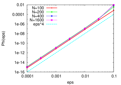
(a) Initial data 1

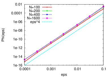
(b) Initial data 2

Figure 2. $p$-system: space integral of the relative entropy $\phi^{\varepsilon}$ with respect to $\varepsilon$ in log scale.

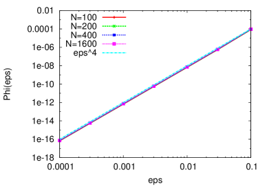
(a) Initial data 1

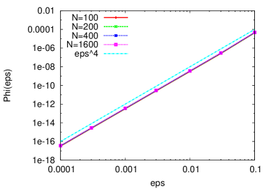
(b) Initial data 2

Figure 3. Goldstein-Taylor model: space integral of the relative entropy $\phi^{\varepsilon}$ with respect to $\varepsilon$ in log scale.

In [19], the authors also apply their relative entropy method to other systems, leading to the same kind of estimates. To conclude this section, we also extend the numerical scheme (4.1)-(4.2) to approximate the weak solutions of both isentropic Euler system and visco-elastic system with memory as considered in [19]. Concerning the isentropic Euler equation, the adopted scaled system is the following:

$$\left\{\begin{aligned} &\partial_{t}\rho^{\varepsilon}+\partial_{x}(\rho^{\varepsilon}u^{\varepsilon})=0,\\ &\partial_{t}(\rho^{\varepsilon}u^{\varepsilon})+\partial_{x}\left(\rho^{\varepsilon}(u^{\varepsilon})^{2}\right)+\frac{1}{\varepsilon^{2}}\partial_{x}p(\rho^{\varepsilon})=-\frac{\sigma}{\varepsilon^{2}}\rho^{\varepsilon}u^{\varepsilon},\end{aligned}\right.\quad(x,t)\in\mathbb{R}\times\mathbb{R}_{+}.$$

The corresponding asymptotic regime in the limit $\varepsilon\to 0$ is given by:

$$\left\{\begin{aligned} &\partial_{t}\overline{\rho}-\partial_{xx}p(\bar{\rho})=0,\\ &\partial_{x}p(\bar{\rho})=-\sigma\bar{\rho}\bar{u},\end{aligned}\right.\quad(x,t)\in\mathbb{R}\times\mathbb{R}_{+}.$$

Similarly, the visco-elastic system reads as follows:

$$\left\{\begin{aligned} &\partial_{t}u^{\varepsilon}-\partial_{x}v^{\varepsilon}=0,\\ &\partial_{t}v^{\varepsilon}-\partial_{x}\gamma(u^{\varepsilon})-\partial_{x}z^{\varepsilon}=0,\\ &\partial_{t}z^{\varepsilon}-\frac{\mu}{\varepsilon^{2}}\partial_{x}v^{\varepsilon}=-\frac{\sigma}{\varepsilon^{2}}z^{\varepsilon},\end{aligned}\right.\quad(x,t)\in\mathbb{R}\times\mathbb{R}_{+},$$

where the asymptotic regime satisfies the following system:

$$\left\{\begin{aligned} &\partial_{t}\overline{u}-\partial_{x}\bar{v}=0,\\ &\partial_{t}\bar{v}-\partial_{x}\gamma(\bar{u})=\mu\partial_{xx}\bar{v},\\ &\mu\partial_{x}\bar{v}=\sigma\bar{z},\end{aligned}\right.\quad(x,t)\in\mathbb{R}\times\mathbb{R}_{+}.$$

The numerical results are displayed Figures 4 and 5. We still observe a convergence rate in $O(\varepsilon^{4})$, which is in good agreement with results established Theorem 3.1 (see also [19]).

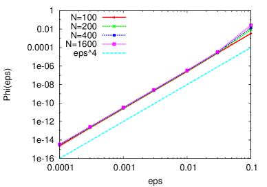
(a) Discontinuous initial data

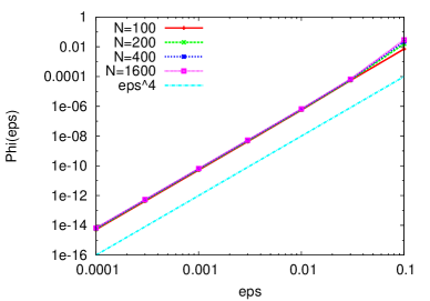
(b) Smooth initial data

Figure 4. Isentropic Euler system: space integral of the relative entropy $\phi^{\varepsilon}$ with respect to $\varepsilon$ in log scale.

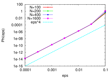
(a) Discontinuous initial data

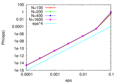
(b) Smooth initial data

Figure 5. Visco-elastic model: space integral of the relative entropy $\phi^{\varepsilon}$ with respect to $\varepsilon$ in log scale.

Acknowledgements. The authors thank the project ANR-12-IS01-0004 GeoNum and the project ANR-14-CE25-0001 Achylles for their partial financial contributions.

References

• [1] C. Berthon and R. Turpault. Asymptotic preserving HLL schemes. Numer. Methods Partial Differential Equations, 27:1396–1422, 2011.
• [2] S. Bianchini, B. Hanouzet, and R. Natalini. Asymptotic behavior of smooth solutions for partially dissipative hyperbolic systems with a convex entropy. Comm. Pure Appl. Math., 60(11):1559–1622, 2007.
• [3] F. Blachère and R. Turpault. An admissibility and asymptotic-preserving scheme for systems of conservation laws with source term on 2D unstructured meshes. Journal of Computational Physics, 2016.
• [4] C. Buet, B. Després, and E. Franck. Design of asymptotic preserving finite volume schemes for the hyperbolic heat equation on unstructured meshes. Numerische Mathematik, 122(2):227–278, 2012.
• [5] C. Buet, B. Després, E. Franck, and T. Leroy. Proof of uniform convergence for a cell-centered AP discretization of the hyperbolic heat equation on general meshes. Math. of Comp., 2016.
• [6] C. Cancès, H. Mathis, and N. Seguin. Relative entropy for the finite volume approximation of strong solutions to systems of conservation laws. Submitted.
• [7] C. Christoforou and A. Tzavaras. Relative entropy for hyperbolic-parabolic systems and application to the constitutive theory of thermoviscoelasticity. ArXiv e-prints, March 2016.
• [8] C. M. Dafermos. The second law of thermodynamics and stability. Arch. Rational Mech. Anal., 70(2):167–179, 1979.
• [9] C. M. Dafermos. Hyperbolic conservation laws in continuum physics, volume 325 of Grundlehren der Mathematischen Wissenschaften [Fundamental Principles of Mathematical Sciences]. Springer-Verlag, Berlin, third edition, 2010.
• [10] R. J. DiPerna. Uniqueness of solutions to hyperbolic conservation laws. Indiana Univ. Math. J., 28(1):137–188, 1979.
• [11] L. Gosse and G. Toscani. An asymptotic-preserving well-balanced scheme for the hyperbolic heat equations. C. R. Math. Acad. Sci. Paris, 334(4):337 – 342, 2002.
• [12] L. Gosse and G. Toscani. Space localization and well-balanced schemes for discrete kinetic models in diffusive regimes. SIAM J. Numer. Anal., 41(2):641–658 (electronic), 2003.
• [13] A. Harten, P. D. Lax, and B. van Leer. On upstream differencing and Godunov-type schemes for hyperbolic conservation laws. SIAM Rev., 25(1):35–61, 1983.
• [14] L. Hsiao and T.-P. Liu. Convergence to nonlinear diffusion waves for solutions of a system of hyperbolic conservation laws with damping. Comm. Math. Phys., 143(3):599–605, 1992.
• [15] S. Jin. Efficient asymptotic-preserving (AP) schemes for some multiscale kinetic equations. SIAM J. Sci. Comput., 21(2):441–454 (electronic), 1999.
• [16] S. Jin, L. Pareschi, and G. Toscani. Diffusive relaxation schemes for multiscale discrete-velocity kinetic equations. SIAM J. Numer. Anal., 35(6):2405–2439, 1998.
• [17] V. Jovanović and C. Rohde. Error estimates for finite volume approximations of classical solutions for nonlinear systems of hyperbolic balance laws. SIAM J. Numer. Anal., 43(6):2423–2449 (electronic), 2006.
• [18] Shuichi Kawashima. Large-time behaviour of solutions to hyperbolic-parabolic systems of conservation laws and applications. Proc. Roy. Soc. Edinburgh Sect. A, 106(1-2):169–194, 1987.
• [19] C. Lattanzio and A.E. Tzavaras. Relative entropy in diffusive relaxation. SIAM J. Math. Anal., 45(3):1563–1584, 2013.
• [20] P.L. Lions and G. Toscani. Diffusive limit for finite velocity Boltzmann kinetic models. Revista Matematica Iberoamericana, 13(3):473–514, 1997.
• [21] P. Marcati, A.J. Milani, and P. Secchi. Singular convergence of weak solutions for a quasilinear nonhomogeneous hyperbolic system. Manuscripta Math., 60(1):49–69, 1988.
• [22] M. Mei. Best asymptotic profile for hyperbolic $p$-system with damping. SIAM J. Math. Anal., 42(1):1–23, 2010.
• [23] G. Naldi and L. Pareschi. Numerical schemes for kinetic equations in diffusive regimes. Appl. Math. Lett., 11(2):29–35, 1998.
• [24] G. Naldi and L. Pareschi. Numerical schemes for hyperbolic systems of conservation laws with stiff diffusive relaxation. SIAM J. Numer. Anal., 37(4):1246–1270, 2000.
• [25] K. Nishihara. Convergence rates to nonlinear diffusion waves for solutions of system of hyperbolic conservation laws with damping. J. Differential Equations, 131(2):171 – 188, 1996.
• [26] K. Nishihara. Asymptotic behavior of solutions of quasilinear hyperbolic equations with linear damping. J. Differential Equations, 137(2):384–395, 1997.
• [27] K. Nishihara, W. Wang, and T. Yang. $L_{p}$-convergence rate to nonlinear diffusion waves for $p$-system with damping. J. Differential Equations, 161(1):191–218, 2000.
• [28] A. E. Tzavaras. Relative entropy in hyperbolic relaxation. Commun. Math. Sci., 3(2):119–132, 2005.
• [29] C. J. van Duyn and L. A. Peletier. A class of similarity solutions of the nonlinear diffusion equation. Nonlinear Anal., 1(3):223–233, 1976/77.
• [30] C. J. van Duyn and L. A. Peletier. Asymptotic behaviour of solutions of a nonlinear diffusion equation. Arch. Ration. Mech. Anal., 65(4):363–377, 1977.