September 6th 2016

THE 1-LOOP VACUUM POLARIZATION FOR A GRAPHENE-LIKE MEDIUM IN AN EXTERNAL MAGNETIC FIELD ; CORRECTIONS TO THE COULOMB POTENTIAL

B. Machet

Abstract: I calculate the 1-loop vacuum polarization $\Pi_{\mu\nu}(k,B,a)$ for a photon of momentum $k=(\hat{k},k_{3})$ interacting with the electrons of a thin medium of thickness $2a$ simulating graphene, in the presence of a constant and uniform external magnetic field $B$ orthogonal to it (parallel to $k_{3}$). Calculations are done with the techniques of Schwinger, adapted to the geometry and Hamiltonian under scrutiny. The situation gets more involved than for the electron self-energy because the photon is now allowed to also propagate outside the medium. This makes $\Pi_{\mu\nu}$ factorize into a quantum, “reduced” $T_{\mu\nu}(\hat{k},B)$ and a transmittance function $V(k,a)$, in which the geometry of the sample and the resulting confinement of the $\gamma\,e^{+}\,e^{-}$ vertices play major roles. This drags the results away from reduced QED₃₊₁ on a 2-brane. The finiteness of $V$ at $k^{2}=0$ is an essential ingredient to fulfill suitable renormalization condition for $\Pi_{\mu\nu}$ and to fix the corresponding counterterms. Their connection with the transversality of $\Pi_{\mu\nu}$ is investigated. The corrections to the Coulomb potential and their dependence on $B$ strongly differ from QED₃₊₁.

PACS: 12.15.Lk, 12.20.Ds,75.70.Ak

1 Generalities. Framework of the calculations

This study concerns the propagation of a photon (with incoming momentum $k$) interacting with electrons belonging to a graphene-like medium of thickness $2a$, and, more specially, the 1-loop quantum corrections to its propagator.. They originate from the creation, inside the medium, of virtual $e^{+}e^{-}$ pairs which propagate before annihilating, again inside graphene. The two $\gamma\,e^{+}e^{-}$ vertices are therefore geometrically constrained to lie in the interval $[-a,+a]$ along the direction $z$ of the magnetic field, perpendicular to the surface of graphene. This is best expressed by evaluating the photon propagator in position space, and by integrating the “$z$” coordinates of the two vertices from $-a$ to $+a$ instead of the infinite interval of usual Quantum Field Theory (QFT).

The second feature that is implemented to mimic graphene is to deprive the Hamiltonian of the Dirac electrons of its “$\gamma_{3}p_{3}$” term (see for example [3]). I shall not consider a Fermi velocity different from the speed of light, nor additional degeneracies that usually take place in graphene, and will furthermore consider electrons to have a mass $m$, that I shall let go to $0$ at the end of the calculations.

The setting is the following. The constant and uniform magnetic field $\vec{B}$ is chosen to be parallel to the $z$ axis and the wave vector $\vec{k}$ of the propagating photon to lie in the $(x,z)$ plane (see Figure 1) .

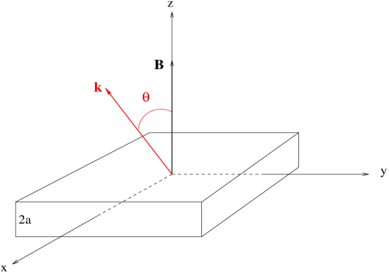
Figure 1: $\vec{B}$ is perpendicular to the medium strip of width $2a$.

The $(\vec{B},\vec{k})$ angle $\theta$ is the “angle of incidence”; the plane $(x,z)$ is the plane of incidence.

Calculations are performed with the techniques of Schwinger for Quantum Field Theory in the presence of a constant and uniform external magnetic field [4] [5]. They have been intensely used by Tsai in standard QED (see for example [6]). Very careful and precise explanations of these techniques have been given in the book by Dittrich and Reuter [7], of invaluable help.

I shall in the following use “hatted” letters for vectors living in the Lorentz subspace $(0,1,2)$ ($0$ being the time-like component, $1$, $2$ and $3$ respectively the $x$, $y$ and $z$-like ones). For example

$$\hat{k}=(k^{0},k^{1},k^{2},0),\quad k=(\hat{k},k_{3})=(k_{0},k_{1},k_{2},k_{3})=(k_{0},\vec{k}).$$ (1)

Dirac $\gamma$ matrices and spinors are always 4-dimensional. Throughout the paper I use the metric $(-1,+1,+1,+1)$ like in [4], [5], [6] and [7].

I shall also use the following notations

$$\begin{split}&k_{\parallel}=(k_{0},0,0,k_{3})\Rightarrow k_{\parallel}^{2}=-k_{0}^{2}+k_{3}^{2},\cr&\hat{k}_{\parallel}=(k_{0},0,0,0)\Rightarrow\hat{k}_{\parallel}^{2}=-k_{0}^{2},\cr&k_{\perp}=(0,k_{1},k_{2},0)=\hat{k}_{\perp}\Rightarrow k_{\perp}^{2}=k_{1}^{2}+k_{2}^{2}=\hat{k}_{\perp}^{2},\cr&g^{\mu\nu}_{\parallel}=(-1,0,0,1),\quad g^{\mu\nu}_{\perp}=(0,1,1,0),\cr&\hat{g}^{\mu\nu}=(-1,1,1,0),\quad\hat{g}^{\mu\nu}_{\parallel}=(-1,0,0,0),\quad\hat{g}^{\mu\nu}_{\perp}=(0,1,1,0)=g^{\mu\nu}_{\perp},\end{split}$$ (2)

and $\sigma^{3}=\sigma^{12}=\frac{i}{2}[\gamma^{1},\gamma^{2}]=diag(1,-1,1,-1)$ like in [7] (it should not be confused with the $2\times 2$ Pauli matrix).

When they are not needed, the factors $\hbar$ and $c$ will very often be skipped.

The plan of this work is the following.

$\bullet$ In section 2, I show, by working in position space, how, due to the confinement of the $\gamma e^{+}e^{-}$ vertices inside the thin medium, the vacuum polarization $\Pi_{\mu\nu}(k,B)$ factorizes into a transmittance function $V(k,a)$ times a “reduced” $T_{\mu\nu}(\hat{k},B)$; after giving an analytical expression for $V$, I show its finiteness on mass-shell ($k^{2}=0$), which is, as shown later, essential for renormalization; I also study its limit as $k_{0}\to 0$, which is useful when calculating the corrections to the Coulomb potential.

$\bullet$ In section 3, I get the unrenormalized $T_{\mu\nu}^{bare}$ as a double integral; it is only $(2+1)$-transverse.

$\bullet$ In section 4, I determine counterterms in order that on mass-shell renormalization conditions for $\Pi_{\mu\nu}(k,B)$ are satisfied. Only $(2+1)$-transversality is achieved. The limits $B=0$ and $B\to\infty$ are studied in detail. Their massless limit $m\to 0$ is smooth. $\Pi_{\mu\nu}$ is shown to vanish at $m=0,B\to\infty$.

$\bullet$ In section 5, I calculate, at the limit $a\to 0$, shown to be smooth, the corrections to the Coulomb potential. I first show that, at $B=0$, it gets renormalized by $1/(1+\alpha/2)$ while, at $B\to\infty$, the genuine Coulomb potential is recovered. The interpolation between these two limits being smooth, sizable deviations from Coulomb are only expected for strongly coupled systems.

$\bullet$ In section 6, I investigate whether, while still preserving on mass-shell renormalization conditions, counterterms can be adapted such that $(3+1)$-transversality is achieved. A fist example introduces extra $B$-independent counterterms. $(3+1)$-transversality is achieved at $B=0$ only; at $B\to\infty$, $\Pi_{\mu\nu}$ does not vanish anymore at $m=0$. In the second example, arguing that, de facto, by neglecting $B$-dependent boundary terms, Schwinger introduces $B$-dependent counterterms, I introduce counterterms that depend on the external $B$. At this price, $(3+1)$-transversality can be achieved at any $B$ while $\Pi_{\mu\nu}$ vanishes at $B\to\infty$ independently of the limit $m\to 0$.

$\bullet$ Section 7 concludes this works with general remarks concerning the calculation, the fate of dimensional reduction which is a well known phenomenon for QED₃₊₁ in superstrong external $B$, and states numerous issues that have not been tackled here and should be in future works.

$\bullet$ The demonstration of the master factorization formula $\Pi_{\mu\nu}\sim VT_{\mu\nu}$ in position space, eq. (10), is detailed in Appendix A.

Like in [8] and [9], calculations are exposed in details, with no “gap”, such that it should not be a problem for a dedicated reader to redo them.

2 The photon propagator in $\boldsymbol{x}$-space and the vacuum polarization $\boldsymbol{\Pi^{\mu\nu}}$ ; generalities

Figure 2: The vacuum polarization $\Pi^{\mu\nu}(k)$.

The 1-loop vacuum polarization $\Pi_{\mu\nu}$ we determine by calculating the photon propagator in position-space, while confining, at the two vertices $\gamma\,e^{+}e^{-}$, the corresponding $z$ coordinates inside graphene, $z\in[-a,a]$.

It factorizes into $\Pi_{\mu\nu}(\hat{k},k_{3},\displaystyle\frac{y_{3}}{a},B)=\displaystyle\frac{1}{\pi^{2}}\;T_{\mu\nu}(\hat{k},B)\;U(\hat{k},k_{3},\displaystyle\frac{y_{3}}{a})$ in which $U$ is a universal function that does not depend on the magnetic field, nor on $\alpha\equiv\displaystyle\frac{e^{2}}{4\pi(\hbar c)}$, that we also encounter when no external $B$ is present. $U$ turns out (see eq. (21) below) to be the Fourier transform of the product of two functions: the first, $\displaystyle\frac{\sin al_{3}}{al_{3}}$, is itself the Fourier transform of the “gate function” corresponding to the graphene strip along $z$; the second carries the remaining information attached to the confinement of the vertices.

The integration variable $l_{3}$ of this Fourier transform is the component along $B$ of the difference $s-k$ between the momenta of the outgoing and incoming photons. It represents the amount of momentum non-conservation of photons due to the exchange between them and (the quantum momentum fluctuations of) electrons.

This factorization can be traced back to $T_{\mu\nu}$ not depending on $k_{3}$, for the simple reason that the propagators of electrons inside graphene should be evaluated at vanishing momentum along $z$.

An example of how factors combine is the following. $\Pi_{\mu\nu}$ still includes an integration on the loop momentum $p_{3}$, which factors out. That the interactions of electrons are confined along $B$ triggers quantum fluctuations of their momentum in this direction. Setting an ultraviolet cutoff $\pm\displaystyle\frac{\hbar}{a}$ on the $p_{3}$ integration (saturating the Heisenberg uncertainty relation) makes this integral proportional to $\displaystyle\frac{1}{a}$. This factor completes, inside the integral $\int dl_{3}$ defining $U$, the “geometric” $\displaystyle\frac{\sin al_{3}}{al_{3}}$ evoked above. Then, the integration $\int dl_{3}$ gets bounded by the rapid decrease of $\displaystyle\frac{\sin al_{3}}{al_{3}}$ for $|l_{3}|$ larger than $\displaystyle\frac{\hbar}{a}$; this upper bound $|l_{3}|\leq\displaystyle\frac{\hbar}{a}$ is the same as the one that we set for quantum fluctuations of the electron momentum along $z$. Therefore, the energy-momentum non-conservation between the outgoing and incoming photons cannot exceed the uncertainty on the momentum of electrons due to the confinement of vertices. Exact momentum conservation for the photon only gets recovered when $a\to\infty$ (limit of “standard” QFT).

2.1 The 1-loop photon propagator in position space

I calculate the 1-loop photon propagator (eq. (4.1) of [7])

$$\Delta^{\rho\sigma}(x,y)=i\,<0\;|\;TA^{\rho}(x)A^{\sigma}(y)\;|\;0>,$$ (3)

and somewhat lighten the notations, often omitting symbols like T-product, …, writing for example $G(\hat{k})$ instead of $G(\hat{k},B)$.

Introducing the coordinates $u=(u_{0},u_{1},u_{2},u_{3})$ and $v=(v_{0},v_{1},v_{2},v_{3})$ of the two $\gamma\,e^{+}e^{-}$ vertices one gets at 1-loop

$$\Delta^{\rho\sigma}(x,y)=i\int d^{4}u\int d^{4}v\;A^{\rho}(x)\big{[}(-ie)A^{\mu}(u)\bar{\psi}(u)\gamma_{\mu}\psi(u)\big{]}\big{[}(-ie)A^{\nu}(v)\bar{\psi}(v)\gamma_{\nu}\psi(v)\big{]}A^{\sigma}(y).$$ (4)

Making the contractions for fermions etc …yields

$$\begin{split}\Delta^{\rho\sigma}(x,y)&=ie^{2}\int d^{4}u\int d^{4}v\;Tr\int\frac{d^{4}k}{(2\pi)^{4}}\;e^{ik(u-x)}\Delta^{\rho\mu}(k)\gamma_{\mu}\Phi(u,v)\int\frac{d^{4}p}{(2\pi)^{4}}\;e^{ip(u-v)}G(p)\gamma_{\nu}\cr&\hskip 85.35826pt\Phi(v,u)\int\frac{d^{4}r}{(2\pi)^{4}}\;e^{ir(v-u)}G(r)\int\frac{d^{4}s}{(2\pi)^{4}}\;e^{is(y-v)}\Delta^{\sigma\nu}(s).\end{split}$$ (5)

In what follows we shall also often omit the trace symbol “$Tr$”.

I have inserted in (5) the phase $\Phi$ that occurs in a fermion propagator $G$ in the presence of a constant external magnetic field [7]

$$\begin{split}G(x^{\prime},x^{\prime\prime})&=\Phi(x^{\prime},x^{\prime\prime})\int\frac{d^{4}p}{(2\pi)^{4}}\;e^{ip(x^{\prime}-x^{\prime\prime})}G(p),\cr\Phi(x^{\prime},x^{\prime\prime})&=\exp\Big{[}-ie\int_{x^{\prime\prime}}^{x^{\prime}}dx_{\mu}\;\big{(}A^{\mu}(x)+\frac{1}{2}F^{\mu\nu}(x^{\prime}_{\nu}-x^{\prime\prime}_{\nu})\big{)}\Big{]}.\end{split}$$ (6)

Since the curl of the integrand vanishes, the integral inside the phase is independent of the path of integration, which can therefore be chosen as straight $x(t)=x^{\prime\prime}+t(x^{\prime}-x^{\prime\prime}),t\in[0,1]$, leading to the familiar expression

$$\Phi(x^{\prime},x^{\prime\prime})=\exp\Big{[}ie\int_{x^{\prime\prime}}^{x^{\prime}}dx_{\mu}\;A^{\mu}(x)\Big{]}.$$ (7)

This is the last time that we mention $\Phi$ because it goes away when the path of integration closes, which is the case for the vacuum polarization.

2.1.1 “Standard” $\boldsymbol{(3+1)}$-Quantum Field Theory

One integrates $\int_{-\infty}^{+\infty}d^{4}u$ and $\int_{-\infty}^{+\infty}d^{4}v$ for the four components of $u$ and $v$. This gives:

$$\Delta^{\rho\sigma}(x,y)=i\int\frac{d^{4}k}{(2\pi)^{4}}\;e^{-ik(x-y)}\Delta^{\rho\mu}(k)\Delta^{\nu\sigma}(k)\underbrace{e^{2}\int\frac{d^{4}p}{(2\pi)^{4}}\;\gamma_{\mu}G(p)\gamma_{\nu}G(p+k)}_{i\Pi_{\mu\nu}(k)}.$$ (8)

To obtain the sought for vacuum polarization, the two external photon propagators $\Delta^{\rho\mu}(k)$ and $\Delta^{\nu\sigma}(k)$ have to be chopped off, which gives the customary expression

$$i\Pi_{\mu\nu}(k)=e^{2}\int\frac{d^{4}p}{(2\pi)^{4}}\;\gamma_{\mu}\,G(p)\,\gamma_{\nu}\,G(p+k).$$ (9)

2.1.2 The case of a graphene-like medium: the $\boldsymbol{\gamma\,e^{+}e^{-}}$ vertices are confined along $\boldsymbol{z}$

The coordinates $u_{3}$ and $v_{3}$ of the two vertices we do not integrate anymore $\int_{-\infty}^{+\infty}$ but only $\int_{-a}^{+a}$. This localizes the interactions of electrons with photons inside graphene. It has been shown in [8] that, in the case of the electron self-energy at 1-loop. this procedure leads to the same result as reduced QED₃₊₁ on a 2-brane [10] [11].

Decomposing in (5) $du=d^{3}\hat{u}\,du_{3},\;dv=d^{3}\hat{v}\,dv_{3}$, we get by standard manipulations (see Appendix A)

$$\begin{split}\Delta^{\rho\sigma}(x,y)&=i\int\frac{dp_{3}}{2\pi}\int\frac{dk_{3}}{2\pi}\int\frac{dr_{3}}{2\pi}\int\frac{ds_{3}}{2\pi}\int_{-a}^{+a}du_{3}\;e^{iu_{3}(k_{3}+p_{3}-r_{3})}\int_{-a}^{+a}dv_{3}\;e^{iv_{3}(-p_{3}+r_{3}-s_{3})}\cr&\int\frac{d^{3}\hat{k}}{(2\pi)^{3}}\;e^{i\hat{k}(\hat{y}-\hat{x})}e^{ik_{3}(-x_{3})}e^{is_{3}(y_{3})}\Delta^{\rho\mu}(\hat{k},k_{3})\Delta^{\sigma\nu}(\hat{k},s_{3})\ \underbrace{e^{2}\int\frac{d^{3}\hat{p}}{(2\pi)^{3}}\;\gamma_{\mu}G(\hat{p},B)\gamma_{\nu}G(\hat{p}+\hat{k},B)}_{iT_{\mu\nu}(\hat{k},B)},\end{split}$$ (10)

in which we introduced the tensor $T_{\mu\nu}(\hat{k},B)$ that is calculated in section 3.

One of the main difference with standard QFT (subsection 2.1.1) is that the tensor $T_{\mu\nu}$ does not depend on $k_{3}$, but only on $\hat{k}$. The reason is that, as already mentioned, the propagators of electrons in the loop are evaluated at vanishing momentum in the direction of $B$, simulating a graphene-like Hamiltonian.

Notice that, despite the “classical” input $p_{3}=0$ the photon propagator still involves an integration $\int dp_{3}$ over the loop momentum $p_{3}$.

Now,

$$\int_{-a}^{+a}dx\;e^{itx}=2\;\frac{\sin at}{t},$$ (11)

such that

$$\begin{split}&\Delta^{\rho\sigma}(x,y)=4i\int\frac{dk_{3}}{2\pi}\int\frac{ds_{3}}{2\pi}e^{i(s_{3}y_{3}-k_{3}x_{3})}L(a,s_{3},k_{3})\int\frac{d^{3}\hat{k}}{(2\pi)^{3}}\;e^{i\hat{k}(\hat{y}-\hat{x})}\Delta^{\rho\mu}(\hat{k},k_{3})\Delta^{\sigma\nu}(\hat{k},s_{3})\;iT_{\mu\nu}(\hat{k},B),\cr&\hskip 85.35826pt\text{with}\quad L(a,s_{3},k_{3})=\int_{-\infty}^{+\infty}\frac{dp_{3}}{2\pi}\frac{dr_{3}}{2\pi}\;\frac{\sin a(k_{3}+p_{3}-r_{3})}{k_{3}+p_{3}-r_{3}}\;\frac{\sin a(r_{3}-p_{3}-s_{3})}{r_{3}-p_{3}-s_{3}}.\end{split}$$ (12)

Going from the variables $r_{3},p_{3}$ to the variables $p_{3},h_{3}=r_{3}-p_{3}$ leads to

$$L(a,s_{3},k_{3})=\int_{-\infty}^{+\infty}\frac{dp_{3}}{2\pi}\;K(a,s_{3},k_{3}),\quad\text{with}\quad K(a,s_{3},k_{3})=\int_{-\infty}^{+\infty}\frac{dh_{3}}{2\pi}\;\frac{\sin a(k_{3}-h_{3})}{k_{3}-h_{3}}\;\frac{\sin a(h_{3}-s_{3})}{h_{3}-s_{3}},$$ (13)

and the photon propagator at 1-loop writes

$$\begin{split}\hskip-28.45274pt\Delta^{\rho\sigma}(a,x,y)&=4i\int_{-\infty}^{+\infty}\frac{d^{3}\hat{k}}{(2\pi)^{3}}\,e^{i\hat{k}(\hat{y}-\hat{x})}\int_{-\infty}^{+\infty}\frac{ds_{3}}{2\pi}\int_{-\infty}^{+\infty}\frac{dk_{3}}{2\pi}\;e^{i(s_{3}y_{3}-k_{3}x_{3})}\,\Delta^{\rho\mu}(\hat{k},k_{3})\;K(a,s_{3},k_{3})\;\Delta^{\nu\sigma}(\hat{k},s_{3})\;\mu\,T_{\mu\nu}(\hat{k},B),\cr&\hskip 56.9055pt\text{in which}\quad\mu\equiv\int_{-\infty}^{+\infty}\frac{dp_{3}}{2\pi}\quad\text{factors out}.\end{split}$$ (14)

Last, going to the variable $l_{3}=s_{3}-k_{3}$ (difference of the momentum along $z$ of the incoming and outgoing photon), one gets

$$K(a,s_{3},k_{3})\equiv\tilde{K}(a,l_{3})=\frac{1}{2}\frac{\sin a(s_{3}-k_{3})}{s_{3}-k_{3}}=\frac{1}{2}\frac{\sin al_{3}}{l_{3}}.$$ (15)

To define the vacuum polarization $\Pi_{\mu\nu}$ from (14) and (15) we proceed like with (8) in standard QFT by chopping the two external photon propagators $\Delta^{\rho\mu}(k)\equiv\Delta^{\rho\mu}(\hat{k},k_{3})$ and $\Delta^{\nu\sigma}(k)\equiv\Delta^{\nu\sigma}(\hat{k},k_{3})$ off $\Delta^{\rho\sigma}$. The mismatch between $\Delta^{\nu\sigma}(\hat{k},k_{3})$ and $\Delta^{\nu\sigma}(\hat{k},s_{3}\equiv k_{3}+l_{3})$ which occurs in (14) has to be accounted for by writing symbolically (see subsection 2.2.1 for the explicit interpretation) $\Delta^{\nu\sigma}(\hat{k},k_{3}+l_{3})=\Delta^{\nu\sigma}(\hat{k},k_{3})[\Delta^{\nu\sigma}(\hat{k},k_{3})]^{-1}\Delta^{\nu\sigma}(\hat{k},k_{3}+l_{3})$. I therefore rewrite the photon propagator (14) as

$$\begin{split}\Delta^{\rho\sigma}(a,x,y)&=4i\mu\int_{-\infty}^{+\infty}\frac{d^{4}k}{(2\pi)^{4}}\,e^{ik(y-x)}\Delta^{\rho\mu}(k)\;\Delta^{\nu\sigma}(k)\cr&\left[\int_{-\infty}^{+\infty}\frac{dl_{3}}{2\pi}\;e^{il_{3}y_{3}}\,\tilde{K}(a,l_{3})\;[\Delta^{\nu\sigma}(\hat{k},k_{3})]^{-1}\Delta^{\nu\sigma}(\hat{k},k_{3}+l_{3})\right]\;T_{\mu\nu}(\hat{k},B).\end{split}$$ (16)

Cutting off $\Delta^{\rho\mu}$ and $\Delta^{\nu\sigma}$ leads then to the vacuum polarization $\Pi_{\mu\nu}$:

$$\Pi_{\mu\nu}(\hat{k},k_{3},\frac{y_{3}}{a},B)=-4\mu\int_{-\infty}^{+\infty}\frac{dl_{3}}{2\pi}\;e^{il_{3}y_{3}}\,\tilde{K}(a,l_{3})\;[\Delta^{\nu\sigma}(\hat{k},k_{3})]^{-1}\Delta^{\nu\sigma}(\hat{k},k_{3}+l_{3})\;T_{\mu\nu}(\hat{k},B).$$ (17)

The factor $\mu$, defined in (14), associated with the electron loop-momentum along $z$, is potentially ultraviolet divergent and needs to be regularized. In relation with the “confinement” along $z$ of the $\gamma\,e^{+}e^{-}$ vertices, we shall consider that the electron momentum $p_{3}$ undergoes quantum fluctuations

$$\Delta p_{3}\in[-\frac{\hbar}{a},+\frac{\hbar}{a}],$$ (18)

which saturate the Heisenberg uncertainty relation $\Delta x\;\Delta p\geq\hbar$ . The quantum “uncertainty” on the momentum of electrons is therefore, as expected, inversely proportional to their localization in space (at the vertices of their creation or annihilation); it goes to $\infty$ when $a\to 0$ and vice-versa.

This amounts to taking

$$p_{3}^{m}=\frac{\hbar}{a}$$ (19)

as an ultraviolet cutoff for the quantum electron momentum along $z$. Then

$$\mu\approx\frac{1}{2\pi}\;\frac{2\hbar}{a}=\frac{\hbar}{a\pi}.$$ (20)

One gets accordingly, using also the explicit expression (15) for $\tilde{K}(a,k_{3})$, the following expression for the unrenormalized $\Pi_{\mu\nu}$ (that we shall call $\Pi_{\mu\nu}^{bare}$ in section 3)

$$\begin{split}\Pi^{\mu\nu}(\hat{k},k_{3},\frac{y_{3}}{a},B)&=-\frac{1}{\pi^{2}}\;T^{\mu\nu}(\hat{k},B)\times U(\hat{k},k_{3},\frac{y_{3}}{a}),\cr\text{with}\quad U(\hat{k},k_{3},\frac{y_{3}}{a})&=\int_{-\infty}^{+\infty}dl_{3}\;e^{il_{3}y_{3}}\,\frac{\sin al_{3}}{al_{3}}\;[\Delta^{\nu\sigma}(\hat{k},k_{3})]^{-1}\Delta^{\nu\sigma}(\hat{k},k_{3}+l_{3}),\cr\text{and}\quad T_{\mu\nu}(\hat{k},B)&=-ie^{2}\int_{-\infty}^{+\infty}\frac{d^{3}\hat{p}}{(2\pi)^{3}}\;Tr[\gamma_{\mu}G(\hat{p},B)\gamma_{\nu}G(\hat{p}+\hat{k},B)],\end{split}$$ (21)

in which $T^{\mu\nu}(\hat{k},B)$ can be taken out of the integral because it does not depend on $k_{3}$. This is the announced result, that exhibits the transmittance function $U(\hat{k},k_{3},\frac{y_{3}}{a})$, independent of $B$.
* At the limit $a\to\infty$, the position for creation and annihilation of electrons gets an infinite uncertainty but quantum fluctuations of their momentum in the direction of $B$ shrink to zero. Despite the apparent vanishing of $\mu$ at this limit obtained from (20), the calculation remains meaningful. Indeed, the function $\displaystyle\frac{\sin al_{3}}{al_{3}}$ goes then to $\delta(l_{3})$, which corresponds to the conservation of the photon momentum along $z$ (the non-conservation of the photon momentum is thus seen to be directly related to the quantum fluctuations of the electron momentum). This limit also corresponds to “standard” QFT, in which $\hat{K}(x)=\delta(x)\Rightarrow L(a,s_{3},k_{3})=\displaystyle\int_{-\infty}^{+\infty}\displaystyle\frac{dp_{3}}{2\pi}\,\displaystyle\frac{dr_{3}}{2\pi}\;\delta(k_{3}+p_{3}-r_{3})\;\delta(r_{3}-p_{3}-s_{3})=\int\displaystyle\frac{dp_{3}}{2\pi}\;\delta(k_{3}-s_{3})$.

* For $a<\infty$, momentum conservation along $z$ is only approximate: then, the photon can exchange momentum along $z$ with the quantum fluctuations of the electron momentum. In general, the $\displaystyle\frac{\sin al_{3}}{al_{3}}$ occurring in $U$ provides for photons, by its fast decrease, the same cutoff $|l_{3}|\equiv|s_{3}-k_{3}|\leq\displaystyle\frac{\hbar}{a}=p_{3}^{m}$ along $z$ as for electrons.
* The limit $a\to 0$ would correspond to infinitely thin graphene, infinitely accurate positioning of the creation and annihilation of electrons, but to unbounded quantum fluctuations of their momentum along $B$. Since $\displaystyle\frac{\sin x}{x}\to 1$ when $x\to 0$, no divergence can occur as $a\to 0$, despite the apparent divergence of $p_{3}^{m}$ (19) and $\mu$ (20).

By the choice (19), our model gets therefore suitably regularized both in the infrared and in the ultraviolet.

Notice that the 1-loop photon propagator (14) still depends on the difference $\hat{y}-\hat{x}$ but no longer depends on $y_{3}-x_{3}$ only, it is now a function of both $y_{3}$ and $x_{3}$. Once the dependence on $y_{3}-x_{3}$ has been extracted, there is a left-over dependence on $y_{3}$. It is however in practice very weak.

2.2 The transmittance function $\boldsymbol{U(\hat{k},k_{3},\frac{y_{3}}{a})=\frac{1-n^{2}}{a}\;V(n,\theta,\eta,u)}$

2.2.1 The Feynman gauge

We have seen that, when calculating the vacuum polarization (17), the mismatch between $\Delta^{\nu\sigma}(\hat{k},k_{3})$ had to be accounted for. This is most easily done in the Feynman gauge for photons, in which their propagators write

$$\Delta^{\mu\nu}(k)=-i\;\frac{g^{\mu\nu}}{k^{2}}.$$ (22)

The use of a special gauge is certainly abusive, but we take advantage of the gauge invariance of calculations “à la Schwinger”. Making the same type of calculations in a general $R_{\xi}$ gauge would be much more intricate.

Thanks to the absence of “$k^{\mu}k^{\nu}/k^{2}$” terms and as can be easily checked for each component of $\Delta^{\rho\sigma}$,$[\Delta^{\nu\sigma}(\hat{k},k_{3})]^{-1}\Delta^{\nu\sigma}(\hat{k},k_{3}+l_{3})$ can be simply written, then $\displaystyle\frac{k_{0}^{2}-k_{1}^{2}-k_{2}^{2}-k_{3}^{2}}{k_{0}^{2}-k_{1}^{2}-k_{2}^{2}-(k_{3}+l_{3})^{2}}$. Accordingly, the expression for $U$ resulting from (21) that we shall use from now onwards is

$$U(\hat{k},k_{3},\frac{y_{3}}{a})=\int_{-\infty}^{+\infty}dl_{3}\;e^{il_{3}y_{3}}\,\frac{\sin al_{3}}{al_{3}}\;\frac{k_{0}^{2}-k_{1}^{2}-k_{2}^{2}-k_{3}^{2}}{k_{0}^{2}-k_{1}^{2}-k_{2}^{2}-(k_{3}+l_{3})^{2}}.$$ (23)

The analytical properties and pole structure of the integrand in the complex $k_{3}$ plane play, like for the transmittance in optics (or electronics), an essential role. Because they share many similarities, we have given the same name to $U$.

2.2.2 Going to dimensionless variables : $\boldsymbol{U(\hat{k},k_{3},\frac{y_{3}}{a})\to V(n,\theta,\eta,u)}$

Let us go to dimensionless variables. We define ($p_{3}^{m}$ is given in (19))

$$\eta=\frac{k_{0}}{(c)p_{3}^{m}}=\frac{ak_{0}}{(\hbar c)},\quad u=\frac{y_{3}}{a}.$$ (24)

It is also natural to go to the integration variable $\sigma=al_{3}=\displaystyle\frac{l_{3}}{p_{3}^{m}}$, and to make appear the refractive index

$$n=\frac{(c)|\vec{k}|}{k_{0}}.$$ (25)

and the angle of incidence $\theta$ according to

$$k_{2}=0,\quad k_{1}=|\vec{k}|s_{\theta}=nk_{0}s_{\theta},\quad k_{3}=|\vec{k}|c_{\theta}=nk_{0}c_{\theta},\quad\theta\in\;]0,\frac{\pi}{2}[.$$ (26)

This leads to

$$U(\hat{k},k_{3},\frac{y_{3}}{a})=\frac{1-n^{2}}{a}V(n,\theta,\eta,u),\quad V(n,\theta,\eta,u)=\int_{-\infty}^{+\infty}d\sigma\;e^{i\sigma u}\;\frac{\sin\sigma}{\sigma}\frac{1}{1-n^{2}-\frac{\sigma}{\eta}(2n\cos\theta+\frac{\sigma}{\eta})},$$ (27)

and, therefore, to

$$\Pi^{\mu\nu}(\hat{k},k_{3},\frac{y_{3}}{a},B)=-\frac{1}{\pi^{2}}\;T^{\mu\nu}(\hat{k},B)\frac{1-n^{2}}{a}\times V(n,\theta,\eta,u).$$ (28)

I shall also call $V$ the transmittance function.

As already deduced in subsection 2.1.2 from the smooth behavior of the cardinal sine in the expression (21) of $U$, the apparent divergence of (28) at $a\to 0$ is fake; this can be checked by expanding $V$ at small $\eta\equiv ak_{0}$. The expansions always start at ${\cal O}(\eta^{\geq 1})$ (see for example (34)), which cancels the $1/a$ in (28).

Notice that the dependence of $\Pi_{\mu\nu}$ on $k_{3}$ only occurs inside the transmittance $V$.

2.2.3 Analytical expression of the transmittance $\boldsymbol{V}$

$V$ as given by (27) is the Fourier transform of the function $x\mapsto-\displaystyle\frac{\sin x}{x}\,\displaystyle\frac{\eta^{2}}{(x-\sigma_{1})(x-\sigma_{2})}$, in which

$$\sigma_{1}=-\eta\left(nc_{\theta}-\sqrt{1-n^{2}s_{\theta}^{2}}\right),\quad\sigma_{2}=-\eta\left(nc_{\theta}+\sqrt{1-n^{2}s_{\theta}^{2}}\right)$$ (29)

are the poles of the integrand. The Fourier transform of such a product of a cardinal sine with a rational function is well known. The result involves Heavyside functions of the imaginary parts of the poles $\sigma_{1},\sigma_{2}$, noted $\Theta_{i}^{+}$ for $\Theta_{i}(\Im(\sigma_{i}))$ and $\Theta_{i}^{-}$ for $\Theta_{i}(-\Im(\sigma_{i}))$.

$$\hskip-14.22636ptV(n,\theta,\eta,u)=\frac{-\pi\eta^{2}}{\sigma_{1}\sigma_{2}(\sigma_{1}-\sigma_{2})}\left[(\sigma_{1}-\sigma_{2})+\sigma_{2}\big{(}\Theta_{1}^{-}e^{-i\sigma_{1}(1-u)}+\Theta_{1}^{+}e^{+i\sigma_{1}(1+u)}\big{)}-\sigma_{1}\big{(}\Theta_{2}^{-}e^{-i\sigma_{2}(1-u)}+\Theta_{2}^{+}e^{+i\sigma_{2}(1+u)}\big{)}\right].$$ (30)

$\sigma_{1},\sigma_{2}$ are seen to control the behavior of $V$, thus of $n$, which depends on the signs of their imaginary parts.

(30) can also rewrite

$$\begin{split}&\frac{1-n^{2}}{\pi}V(n,\theta,\eta,u)=\cr&\hskip 14.22636pt1+\frac{-\big{(}nc_{\theta}+\sqrt{1-n^{2}s_{\theta}^{2}}\big{)}\big{(}\Theta_{1}^{-}e^{-i\sigma_{1}(1-u)}+\Theta_{1}^{+}e^{i\sigma_{1}(1+u)}\big{)}+\big{(}nc_{\theta}-\sqrt{1-n^{2}s_{\theta}^{2}}\big{)}\big{(}\Theta_{2}^{-}e^{-i\sigma_{2}(1-u)}+\Theta_{2}^{+}e^{i\sigma_{2}(1+u)}\big{)}}{2\sqrt{1-n^{2}s_{\theta}^{2}}},\end{split}$$ (31)

That the Fourier transform is well defined needs in particular that they do not vanish. This requires either $n\not\in{\mathbb{R}}$ or $n\in{\mathbb{R}}$ and $ns_{\theta}>1$.

When $\sigma_{1}$ and $\sigma_{2}$ are real, which occurs for $n\in{\mathbb{R}}$ and $ns_{\theta}<1$, the simplest procedure is to define everywhere in (30) $\Theta(0)=1/2$. One gets then

$$\frac{1-n^{2}}{\pi}\;V(n,\theta,\eta,u)\stackrel{{\scriptstyle\sigma_{1},\sigma_{2}\in{\mathbb{R}}}}{{=}}1+\frac{\sigma_{2}\,\cos\sigma_{1}\;e^{iu\sigma_{1}}-\sigma_{1}\,\cos\sigma_{2}\;e^{iu\sigma_{2}}}{2\eta\sqrt{1-n^{2}s_{\theta}^{2}}}.$$ (32)

2.2.4 An important property of $\boldsymbol{V}$

From (31) one can deduce

$$\frac{1-n^{2}}{\pi}\;V(k^{2}=0)=0.$$ (33)

Indeed, since we are working in a frame in which $k_{2}=0$, $k^{2}=0\Leftrightarrow k_{0}^{2}-k_{1}^{2}=k_{3}^{2}$. From the definition of $n$ and $\theta$, $nc_{\theta}=\displaystyle\frac{k_{3}}{k_{0}},ns_{\theta}=\displaystyle\frac{k_{1}}{k_{0}}$, which entails $\sigma_{1}=0$ and $\sigma_{2}=-2\eta k_{3}$. Both being real entails in particular that the arguments of all $\Theta$’s in (31) are vanishing, such that they all should consistently be taken to $1/2$. This yields accordingly $\displaystyle\frac{1-n^{2}}{\pi}\;V(k^{2}=0)=1+\displaystyle\frac{-(2k_{3})(\displaystyle\frac{1}{2}+\displaystyle\frac{1}{2})+0\times(\ldots)}{2k_{3}}=0$. Since $1-n^{2}=1-\displaystyle\frac{|\vec{k}|^{2}}{k_{0}^{2}}=-\displaystyle\frac{k^{2}}{k_{0}^{2}}$ trivially vanishes at $k^{2}=0$, the important property is that $V$ is not singular at this limit.

The property (33) will prove essential for the renormalization of $\Pi_{\mu\nu}$ (see section 4).

2.2.5 Expansions of $\boldsymbol{V}$ at $\boldsymbol{\eta\equiv ak_{0}\to 0}$

$\bullet$ For $n\in{\mathbb{R}}$ and $ns_{\theta}>1$, the expansion of $V$ at $\eta\sim ak_{0}\ll 1$ writes

$$\begin{split}\Re(V)&=-\frac{\pi}{\sqrt{n^{2}s_{\theta}^{2}-1}}\,\eta+\frac{\pi}{2}(1+u^{2})\,\eta^{2}+{\cal O}(\eta^{3}),\cr\Im(V)&=u\,n\,c_{\theta}\,\frac{\pi}{\sqrt{n^{2}s_{\theta}^{2}-1}}\,\eta^{2}+{\cal O}(\eta^{3}).\end{split}$$ (34)

This is equivalent to

$$\frac{1-n^{2}}{\pi}\;\frac{V}{a}\stackrel{{\scriptstyle a\to 0}}{{\simeq}}-\frac{k_{0}^{2}-|\vec{k}|^{2}}{\sqrt{s_{\theta}^{2}|\vec{k}|^{2}-k_{0}^{2}}}+{\cal O}(a)$$ (35)

which does not vanish when $a\to 0$.

$\bullet$ For $n\in{\mathbb{R}}$ and $ns_{\theta}<1\Leftrightarrow\sigma_{1},\sigma_{2}\in{\mathbb{R}}$, expanding in powers of $\eta=ak_{0}\ll 1$ yields

$$\frac{1-n^{2}}{\pi}\;\frac{V}{a}\stackrel{{\scriptstyle a\to 0}}{{\simeq}}\frac{1}{2}(1-n^{2})(1+u^{2})\frac{\eta^{2}}{a}+{\cal O}(\eta^{3})=\frac{1}{2}(1+u^{2})(k_{0}^{2}-|\vec{k}|^{2})\;a+\ldots$$ (36)

which vanishes when $a\to 0$.

2.3 The limit $\boldsymbol{k_{0}\to 0}$

This limit is necessary for studying the scalar potential (see section 5).

Expanding (31) at $k_{0}\to 0$ yields (we use the notation $\csc\theta=1/\sin\theta$)

$$\begin{split}&\frac{1-n^{2}}{\pi}V\simeq\frac{e^{-a|\vec{k}|(u+1)(\sin\theta+i\cos\theta)}}{2}\left(-1+i\cot\theta+2e^{a|\vec{k}|(u+1)(\sin\theta+i\cos\theta)}-i(-i+\cot\theta)e^{2a|\vec{k}|(u\sin\theta+i\cos\theta)}\right)\cr&\hskip-42.67912pt+\frac{\csc\theta e^{-a|\vec{k}|(u+1)(\sin\theta+i\cos\theta)}\Big{(}i(\cot\theta\csc\theta+a|\vec{k}|(u+1)(\cot\theta+i))+e^{2a|\vec{k}|(u\sin\theta+i\cos\theta)}(a|\vec{k}|(u-1)(1+i\cot\theta)-i\cot\theta\csc\theta)\Big{)}}{4|\vec{k}|^{2}}k_{0}^{2}\cr&+{\cal O}(k_{0}^{3})\end{split}$$ (37)

On the expression above one can in particular confirm that no divergence at $a\to 0$ occurs for $\frac{1-n^{2}}{\pi}\frac{V}{a}$:

$$\frac{1-n^{2}}{\pi}\frac{V}{a}\stackrel{{\scriptstyle k_{0}\to 0,a\to 0}}{{\simeq}}\frac{|\vec{k}|}{\sin\theta}+\frac{\cos 2\theta(\csc\theta)^{3}}{2|\vec{k}|}k_{0}^{2}+{\cal O}(a),$$ (38)

which is the same result as from (35) for $n\in{\mathbb{R}}$ and $ns_{\theta}>1$, in which case $\sigma_{1}$ and $\sigma_{2}$ are complex.

For $\sigma_{1}$ and $\sigma_{2}$ real $n\in{\mathbb{R}}$ and $ns_{\theta}<1$), we have found in (36) that $\frac{1-n^{2}}{\pi}\frac{V}{a}$ vanishes at $a\to 0$. However, $ns_{\theta}<1\Leftrightarrow s_{\theta}<k_{0}/|\vec{k}|\stackrel{{\scriptstyle k_{0}\to 0}}{{\simeq}}0$ such that, in practice, except at $\theta=0$, we can expect a deviation from Coulomb of the scalar potential when $a\to 0$.

3 Calculation of the unrenormalized $\boldsymbol{T_{\mu\nu}^{bare}}$

I shall now calculate $T_{\mu\nu}^{bare}$ obtained in (21). To ease the parallel with [7] we shall switch $k$ to $-k$ and calculate hereafter

$$T_{\mu\nu}^{bare}(\hat{k},B)=-ie^{2}\int_{-\infty}^{+\infty}\frac{d^{3}\hat{p}}{(2\pi)^{3}}\;Tr\big{[}\gamma_{\mu}G(\hat{p},B)\gamma_{\nu}G(\hat{p}-\hat{k},B)\big{]},$$ (39)

which is similar to eq. (4.1) of [7].

The counterterms, which have to be evaluated for $\Pi_{\mu\nu}$, will be dealt with in section 4.

3.1 First steps

The electron propagator in external $B$ inside the graphene-like medium writes (see (2.47b) of [7]) in momentum space

$$\begin{split}&\hskip-56.9055ptG(\hat{p},B)=i\int_{0}^{\infty}ds\;e^{\displaystyle-is\Big{[}m^{2}-i\epsilon+(-p_{0}^{2}+\xcancel{p_{3}^{2}})+\frac{\tan z}{z}(p_{1}^{2}+p_{2}^{2})\Big{]}}\;\frac{e^{\displaystyle iz\sigma^{3}}}{\cos z}\Big{(}m-(-\gamma_{0}p_{0}+\xcancel{\gamma_{3}p_{3}})-\frac{e^{\displaystyle-iz\sigma^{3}}}{\cos z}(\gamma_{1}p_{1}+\gamma_{2}p_{2})\Big{)},\cr\text{with}\ z&=eBs.\end{split}$$ (41)

in which any dependence on $p_{3}$ is set to $0$. As already mentioned, as far as the vacuum polarization is concerned one can forget about the $\Phi$ phases (7).

To calculate $T_{\mu\nu}^{bare}$ we must redo the calculations of p. 56-72 of [7], adapting them to the situation under scrutiny. I shall emphasize the steps that differ.

Introducing the two Schwinger parameters $s_{1}$ for $G(\hat{p})$ and $s_{2}$ for $G(\hat{p}-\hat{k})$ yields the equivalent of (4.5) of [7]

$$\begin{split}&\hskip-28.45274ptT_{\mu\nu}^{bare}(\hat{k},B)=ie^{2}\int_{0}^{\infty}ds_{1}\int_{0}^{\infty}ds_{2}\;<e^{\displaystyle\Big{[}-is_{1}\big{(}m^{2}+\hat{p}_{\parallel}^{2}+\frac{\tan z_{1}}{z_{1}}p_{\perp}^{2}\big{)}-is_{2}\big{(}m^{2}+(\hat{p}-\hat{k})_{\parallel}^{2}+\frac{\tan z_{2}}{z_{2}}(p-k)_{\perp}^{2}\big{)}\Big{]}}\;\frac{1}{\cos z_{1}\cos z_{2}}\cr&Tr\ \Big{[}\gamma_{\mu}\Big{(}\big{(}m-(\gamma p)_{\parallel}\big{)}\;e^{\displaystyle iz_{1}\sigma^{3}}-\frac{(\gamma\hat{p})_{\perp}}{\cos z_{1}}\Big{)}\gamma_{\nu}\Big{(}\big{(}m-(\gamma(\hat{p}-\hat{k}))_{\parallel}\big{)}\;e^{\displaystyle iz_{2}\sigma^{3}}-\frac{(\gamma(p-k))_{\perp}}{\cos z_{2}}\Big{)}\Big{]}>,\end{split}$$ (42)

in which one has now $\hat{p}_{\parallel}^{2}=-p_{0}^{2},\;p_{\perp}^{2}=p_{1}^{2}+p_{2}^{2},\;z_{1}=eBs_{1},\;z_{2}=eBs_{2}$ and, in (4.3) of [7], $\displaystyle\int\frac{d^{4}p}{(2\pi)^{4}}$ must be replaced by $\displaystyle\int\frac{d^{3}p}{(2\pi)^{3}}$, such that the notation $<\quad>$ stands now for

$$<f(\hat{p})>=\int\frac{d^{3}\hat{p}}{(2\pi)^{3}}\;f(\hat{p}).$$ (43)

One makes the change of variables $(z_{1},z_{2})\to(s,v)$ such that

$$\begin{split}&z_{1}=eBs_{1}=eBs\;\frac{1-v}{2}=z\;\frac{1-v}{2}=\xi,\cr&z_{2}=eBs_{2}=eBs\;\frac{1+v}{2}=z\;\frac{1+v}{2}=\eta,\end{split}$$ (44)

that is

$$z=\xi+\eta\Leftrightarrow s=s_{1}+s_{2},\quad v=\frac{\eta-\xi}{\eta+\xi}=\frac{s_{2}-s_{1}}{s_{2}+s_{1}},$$ (45)

and one has

$$\int_{0}^{\infty}ds_{1}\int_{0}^{\infty}ds_{2}=\int_{0}^{\infty}s\;ds\int_{-1}^{+1}\frac{dv}{2}.$$ (46)

$\bullet$ A few steps are necessary to demonstrate (4.9), (4.10), (4.11) of [7], so as to rewrite the exponential function in (42).

* $s_{1}p_{\parallel}^{2}+s_{2}(p-k)_{\parallel}^{2}=s\left(p_{\parallel}-\displaystyle\frac{1+v}{2}k_{\parallel}\right)^{2}+s\displaystyle\frac{1-v^{2}}{4}k_{\parallel}^{2}$;

* $s_{1}\displaystyle\frac{\tan\xi}{\xi}p_{\perp}^{2}+s_{2}\displaystyle\frac{\tan\eta}{\eta}(p-k)_{\perp}^{2}=\displaystyle\frac{1}{eB}\left[\tan\xi p_{\perp}^{2}+\tan\eta(p-k)_{\perp}^{2}\right]=\displaystyle\frac{\tan\xi+\tan\eta}{eB}\left(p_{\perp}-\displaystyle\frac{\tan\eta}{\tan\xi+\tan\eta}k_{\perp}\right)^{2}+\displaystyle\frac{k_{\perp}^{2}}{eB}\displaystyle\frac{\tan\xi\tan\eta}{\tan\xi+\tan\eta}$;

* $\tan\xi\tan\eta=\displaystyle\frac{\cos(\xi-\eta)-\cos(\xi+\eta)}{\cos(\xi-\eta)+\cos(\xi+\eta)}=\displaystyle\frac{\cos zv-\cos z}{\cos zv+\cos z}$;

* $\tan\xi+\tan\eta=\tan(\xi+\eta)(1-\tan\xi\tan\eta=\tan z(1-\tan\xi\tan\eta))$;

* $\displaystyle\frac{\tan\xi\tan\eta}{\tan\xi+\tan\eta}=\displaystyle\frac{coszv-\cos z}{2\sin z}$;

* $\exp\Big{[}\displaystyle\left(-is_{1}(m^{2}+p_{\parallel}^{2})-is_{2}(m^{2}+(p-k)_{\parallel}^{2})-is_{1}(\tan\xi/\xi)p_{\perp}^{2}-is_{2}(\tan\eta/\eta)(p-k)_{\parallel}^{2}\right)\Big{]}\newline =\exp\Big{[}\displaystyle-is\big{(}m^{2}+\frac{1-v^{2}}{4}k_{\parallel}^{2}+(p_{\parallel}-\frac{1+v}{2}k_{\parallel})^{2}\big{)}\Big{]}\times\exp\Big{[}\displaystyle\big{(}-i\frac{\tan\xi+\tan\eta}{eB}\left(p_{\perp}-\frac{\tan\eta}{\tan\xi+\tan\eta}k_{\perp}^{2}\right)^{2}-i\frac{k_{\perp}^{2}}{eB}\frac{\cos zv-\cos z}{2\sin z}\big{)}\Big{]}\break=e^{\displaystyle-is(\varphi_{0}+\varphi_{1})}$,
with $\varphi_{0}=m^{2}+\displaystyle\frac{1-v^{2}}{4}k_{\parallel}^{2}+\displaystyle\frac{\cos zv-\cos z}{2z\sin z}k_{\perp}^{2},\quad\varphi_{1}=\left(p_{\parallel}-\displaystyle\frac{1+v}{2}k_{\parallel}\right)^{2}+\displaystyle\frac{\tan\xi+\tan\eta}{z}\left(p_{\perp}-\displaystyle\frac{\tan\eta}{\tan\xi+\tan\eta}k_{\perp}\right)^{2}$.

In our case, $p_{3}$ and $p_{3}-k_{3}$ have to be set formally to $0$ such that eqs. (4.10) and (4.11) of [7] are replaced by

$$\begin{split}&\varphi_{0}=m^{2}-\frac{1-v^{2}}{4}\;k_{0}^{2}+\frac{\cos zv-\cos z}{2z\sin z}\;k_{\perp}^{2},\cr&\varphi_{1}=-\left(p_{0}-\frac{1+v}{2}k_{0}\right)^{2}+\frac{\tan\xi+\tan\eta}{z}\left(p_{\perp}-\frac{\tan\eta}{\tan\xi+\tan\eta}k_{\perp}\right)^{2}.\end{split}$$ (47)

This leads to the equivalent of eq. (4.12) of [7]

$$\begin{split}T_{\mu\nu}^{bare}(\hat{k},B)&=ie^{2}\int_{0}^{\infty}ds\;s\int_{-1}^{+1}\frac{dv}{2}\;e^{\displaystyle-is\varphi_{0}}\;\frac{1}{\cos\xi\cos\eta}\cr&Tr<e^{\displaystyle-is\varphi_{1}}\;\left\{\gamma_{\mu}\left[(m-\gamma\hat{p}_{\parallel})e^{\displaystyle i\xi\sigma^{3}}\;-\frac{\gamma p_{\perp}}{\cos\xi}\right]\gamma_{\nu}\left[(m-\gamma(\hat{p}-\hat{k})_{\parallel})e^{\displaystyle i\eta\sigma^{3}}\;-\frac{\gamma(p-k)_{\perp}}{\cos\eta}\right]\right\}>.\end{split}$$ (48)

$\bullet$ One now eliminates $\cos\xi\cos\eta$ in terms of $<e^{-is\varphi_{1}}>$ in (48)

$$<e^{-is\varphi_{1}}>=\int\frac{dp_{0}dp_{1}dp_{2}}{(2\pi)^{3}}\;\exp\left[-is\left(-\left(p_{0}-\frac{1+v}{2}k_{0}\right)^{2}+\frac{\tan\xi+\tan\eta}{z}\left(p_{\perp}-\frac{\tan\eta}{\tan\xi+\tan\eta}k_{\perp}\right)^{2}\right)\right].$$ (49)

One can freely shift the integration variables.

$\displaystyle\int_{-\infty}^{+\infty}dx\;e^{\displaystyle-\pm iAx^{2}}=e^{\displaystyle\pm i\pi/4}\sqrt{\displaystyle\frac{\pi}{A}},\ A>0$, therefore, inside (49):

*  $\displaystyle\int\frac{dp_{0}}{2\pi}$ gives $\displaystyle\frac{1}{2\pi}\;e^{\displaystyle+i\pi/4}\;\sqrt{\displaystyle\frac{\pi}{s}}$.
*  $\displaystyle\int\frac{dp_{1}dp_{2}}{(2\pi)^{2}}$ gives $\displaystyle\frac{1}{(2\pi)^{2}}\Big{(}e^{\displaystyle-i\pi/4}\;\sqrt{\displaystyle\frac{\pi z}{s(\tan\xi+\tan\eta)}}\Big{)}^{2}$,
and $<e^{\displaystyle-is\varphi_{1}}>=\displaystyle\frac{1}{(2\pi)^{3}}\;e^{\displaystyle-i\pi/4}\;z\left(\displaystyle\frac{\pi}{s}\right)^{3/2}\displaystyle\frac{1}{\tan\xi+\tan\eta}$.

One then uses $\tan\xi+\tan\eta=\displaystyle\frac{\sin z}{\cos\xi\cos\eta}$ to get

$$<e^{\displaystyle-is\varphi_{1}}>=\displaystyle\frac{1}{(2\pi)^{3}}\;e^{\displaystyle-i\pi/4}\;\left(\displaystyle\frac{\pi}{s}\right)^{3/2}\displaystyle\frac{z}{\sin z}\;\cos\xi\cos\eta.$$ (50)

In $T_{\mu\nu}$, one can therefore replace $\displaystyle\frac{1}{\cos\xi\cos\eta}$ with $\displaystyle\frac{1}{(2\pi)^{3}}\;e^{\displaystyle-i\pi/4}\;\left(\displaystyle\frac{\pi}{s}\right)^{3/2}\displaystyle\frac{z}{\sin z}\;\displaystyle\frac{1}{<e^{-is\varphi_{1}}>}$ and get

$$\begin{split}T_{\mu\nu}^{bare}(\hat{k},B)&=i\frac{\alpha}{2\pi}\sqrt{\pi}e^{\displaystyle-i\pi/4}\int_{0}^{\infty}\frac{ds}{\sqrt{s}}\int_{-1}^{+1}\frac{dv}{2}\;e^{\displaystyle-is\varphi_{0}}\;\frac{z}{\sin z}\;\frac{1}{<e^{\displaystyle-is\varphi_{1}}>}\cr&\hskip 56.9055ptTr<e^{\displaystyle-is\varphi_{1}}\;\left[\gamma_{\mu}\Big{(}(m-\gamma\hat{p}_{\parallel})e^{\displaystyle i\xi\sigma^{3}}\;-\frac{\gamma p_{\perp}}{\cos\xi}\Big{)}\gamma_{\nu}\Big{(}(m-\gamma(\hat{p}-\hat{k})_{\parallel})e^{\displaystyle i\eta\sigma^{3}}\;-\displaystyle\frac{\gamma(p-k)_{\perp}}{\cos\eta}\Big{)}\right]>,\cr&=\frac{\alpha}{2\pi}\int_{0}^{\infty}\frac{ds}{\sqrt{s}}\int_{-1}^{+1}\frac{dv}{2}\;e^{\displaystyle-is\varphi_{0}}\;\frac{z}{\sin z}\;I_{\mu\nu},\end{split}$$ (51)

with

$$\begin{split}&\hskip-28.45274ptI_{\mu\nu}=i\sqrt{\pi}\;e^{\displaystyle-i\pi/4}\;\displaystyle\frac{1}{<e^{\displaystyle-is\varphi_{1}}>}Tr<e^{\displaystyle-is\varphi_{1}}\;\left[\gamma_{\mu}\Big{(}(m-\gamma\hat{p}_{\parallel})e^{\displaystyle i\sigma^{3}\xi}\;-\displaystyle\frac{\gamma p_{\perp}}{\cos\xi}\Big{)}\gamma_{\nu}\Big{(}(m-\gamma(\hat{p}-\hat{k})_{\parallel})e^{\displaystyle i\sigma^{3}\eta}\;-\displaystyle\frac{\gamma(p-k)_{\perp}}{\cos\eta}\Big{)}\right]>\cr&\hskip-28.45274pt=i\sqrt{\pi}\;e^{\displaystyle-i\pi/4}\;\frac{1}{<e^{\displaystyle-is\varphi_{1}}>}Tr<e^{\displaystyle-is\varphi_{1}}\;\left[\gamma_{\mu}\Big{(}(m+\gamma_{0}p_{0})e^{\displaystyle i\sigma^{3}\xi}\;-\frac{\gamma p_{\perp}}{\cos\xi}\Big{)}\gamma_{\nu}\Big{(}(m+\gamma_{0}(\hat{p}-\hat{k})_{0})e^{\displaystyle i\sigma^{3}\eta}\;-\frac{\gamma(p-k)_{\perp}}{\cos\eta}\Big{)}\right]>.\end{split}$$ (52)

One needs therefore $<e^{\displaystyle-is\varphi_{1}}p_{0}>,<e^{\displaystyle-is\varphi_{1}}p_{0}^{2}>,<e^{\displaystyle-is\varphi_{1}}p_{0}p_{1,2}>,<e^{\displaystyle-is\varphi_{1}}p_{1,2}p_{1,2}>$.

* $<e^{\displaystyle-is\varphi_{1}}\left(p_{0}-\displaystyle\frac{1+v}{2}k_{0}\right)>=0$ because it is an odd integral $\displaystyle\int dp_{0}$.
Therefore, $<e^{\displaystyle-is\varphi_{1}}p_{0}>=\displaystyle\frac{1+v}{2}k_{0}<e^{\displaystyle-is\varphi_{1}}>$;

* $<e^{\displaystyle-is\varphi_{1}}p_{0}^{2}>=<e^{\displaystyle-is\varphi_{1}}\Big{(}p_{0}-\displaystyle\frac{1+v}{2}k_{0}\Big{)}^{2}>+k_{0}(1+v)<e^{\displaystyle-is\varphi_{1}}p_{0}>-\Big{(}\displaystyle\frac{1+v}{2}\Big{)}^{2}k_{0}^{2}<e^{\displaystyle-is\varphi_{1}}>$.

$\displaystyle\int\frac{dp_{1}dp_{2}}{(2\pi)^{2}}\;e^{\displaystyle-is\frac{\tan\xi+\tan\eta}{z}\Big{(}p_{\perp}-\frac{\tan\eta}{\tan\xi+\tan\eta}k_{\perp}\Big{)}^{2}}\displaystyle\int\frac{dp_{0}}{2\pi}\;e^{\displaystyle is\Big{(}p_{0}-\frac{1+v}{2}k_{0}\Big{)}^{2}}\Big{(}p_{0}-\frac{1+v}{2}k_{0}\Big{)}^{2}\newline =\displaystyle\int\frac{dp_{1}dp_{2}}{(2\pi)^{2}}\;e^{\displaystyle-is\frac{\tan\xi+\tan\eta}{z}\Big{(}p_{\perp}-\frac{\tan\eta}{\tan\xi+\tan\eta}k_{\perp}\Big{)}^{2}}\Big{(}-i\displaystyle\frac{1}{2\pi}\displaystyle\frac{d}{ds}e^{\displaystyle i\pi/4}\sqrt{\displaystyle\frac{\pi}{s}}\Big{)}=\displaystyle\int\frac{dp_{0}dp_{1}dp_{2}}{(2\pi)^{3}}\;\displaystyle\frac{i}{2s}e^{\displaystyle-is\varphi_{1}}$.

So, $<e^{\displaystyle-is\varphi_{1}}p_{0}^{2}>=\displaystyle\frac{i}{2s}<e^{\displaystyle-is\varphi_{1}}>+k_{0}^{2}(\frac{1+v}{2})^{2}<e^{-is\varphi_{1}}>$, which agrees with (4.15) in [7] with $g_{\mu\nu}^{\parallel}=g_{00}=-1$.

In a similar way one can get the 3 formulæ (4.15) of [7].

Following [7] let us write (we keep the natural $(-)$ signs in $S_{3}$ and $S_{4}$)

$$\begin{split}I_{\mu\nu}&=i\sqrt{\pi}\;e^{\displaystyle-i\pi/4}\;\displaystyle\frac{1}{<e^{\displaystyle-is\varphi_{1}}>}\sum_{i=1,5}TrS_{i},\cr&\text{with}\cr TrS_{1}&=m^{2}Tr<e^{\displaystyle-is\varphi_{1}}\gamma_{\mu}e^{\displaystyle i\sigma^{3}\xi}\gamma_{\nu}e^{\displaystyle i\sigma^{3}\eta}>,\cr TrS_{2}&=Tr<e^{\displaystyle-is\varphi_{1}}\gamma_{\mu}\gamma_{0}p_{0}e^{\displaystyle i\sigma^{3}\xi}\gamma_{\nu}\gamma_{0}(p_{0}-k_{0})e^{\displaystyle i\sigma^{3}\eta}>,\cr TrS_{3}&=Tr<e^{\displaystyle-is\varphi_{1}}\gamma_{\mu}(-)\gamma_{0}p_{0}e^{\displaystyle i\sigma^{3}\xi}\gamma_{\nu}\gamma(\hat{p}-\hat{k})_{\perp}>\displaystyle\frac{1}{\cos\eta},\cr TrS_{4}&=Tr<e^{\displaystyle-is\varphi_{1}}\gamma_{\mu}\gamma\hat{p}_{\perp}\gamma_{\nu}(-)\gamma_{0}(p_{0}-k_{0})e^{\displaystyle i\sigma^{3}\eta}>\displaystyle\frac{1}{\cos\xi},\cr TrS_{5}&=Tr<e^{\displaystyle-is\varphi_{1}}\gamma_{\mu}\gamma\hat{p}_{\perp}\gamma_{\nu}\gamma(\hat{p}-\hat{k})_{\perp}>\displaystyle\frac{1}{\cos\xi\cos\eta}.\end{split}$$ (53)

Since $\sigma_{3}^{2}=1$, $e^{\displaystyle i\sigma^{3}\xi}=\cos\xi+i\sigma^{3}\sin\xi=\cos\xi-\displaystyle\frac{1}{2}[\gamma_{1},\gamma_{2}]\sin\xi=\cos\xi-\gamma_{1}\gamma_{2}\sin\xi$.

* $TrS_{1}=4m^{2}<e^{\displaystyle-is\varphi_{1}}>\big{[}-\cos z\;g_{\mu\nu}+(g_{\mu 1}g_{\nu 1}+g_{\mu_{2}}g_{\nu 2})(\cos z-\cos zv)+2(g_{\mu 1}g_{\nu 2}-g_{\mu 2}g_{\nu 1})\sin zv\big{]}$.

After integrating $\int dv$, the odd function $\sin zv$ yields a vanishing contribution, such that we can forget it. Furthermore, $g_{\mu 1}g_{\nu 1}+g_{\mu_{2}}g_{\nu 2}=g_{\mu\nu}^{\perp}$ such that, finally

$TrS_{1}=-4m^{2}<e^{\displaystyle-is\varphi_{1}}>\left[g_{\mu\nu}^{\parallel}\cos z+g_{\mu\nu}^{\perp}\cos zv+odd(v)\right]$, which is the result of [7].

* $TrS_{2}$ needs to be re-calculated because the formula $\gamma_{\parallel}^{\lambda}\gamma_{\parallel\lambda}=-2$ used at the end of page 66 of [7] is no longer valid since $\gamma_{\parallel}$ stands now for $\gamma_{0}$ only.

$TrS_{2}=<p_{0}(p_{0}-k_{0})e^{\displaystyle-is\varphi_{1}}>\;Tr\gamma_{\mu}\gamma_{0}e^{\displaystyle i\sigma^{3}\xi}\gamma_{\nu}\gamma_{0}e^{\displaystyle i\sigma^{3}\eta}$ and one uses (4.15) of [7] for the $<\ >$.

This gives

$TrS_{2}=4<e^{\displaystyle-is\varphi_{1}}>\big{(}-k_{0}^{2}\displaystyle\frac{1-v^{2}}{4}+\displaystyle\frac{i}{2s}\big{)}\Big{[}(g_{\mu\nu}+2g_{\mu 0}g_{\nu 0}-g_{\mu 1}g_{\nu 1}-g_{\mu 2}g_{\nu 2})\cos z+(g_{\mu 1}g_{\nu 1}+g_{\mu 2}g_{\nu 2})\cos zv\newline -(g_{\mu 1}g_{\nu 2}-g_{\mu 2}g_{\nu 1})\sin zv\Big{]}$.

Since $g_{\mu\nu}$ is diagonal, $g_{\mu 1}g_{\nu 1}+g_{\mu 2}g_{\nu 2}=g_{\mu\nu}^{\perp}$ such that, dropping like before the function odd in $v$, one gets

$TrS_{2}=4<e^{\displaystyle-is\varphi_{1}}>\big{(}-k_{0}^{2}\displaystyle\frac{1-v^{2}}{4}+\displaystyle\frac{i}{2s}\big{)}\Big{[}(g_{\mu\nu}+2g_{\mu 0}g_{\nu 0}-g_{\mu\nu}^{\perp})\cos z+g_{\mu\nu}^{\perp}\cos zv+odd(v)\Big{]}$

$=4<e^{\displaystyle-is\varphi_{1}}>\big{(}-k_{0}^{2}\displaystyle\frac{1-v^{2}}{4}+\displaystyle\frac{i}{2s}\big{)}\Big{[}(g_{\mu\nu}^{\parallel}+2g_{\mu 0}g_{\nu 0})\cos z+g_{\mu\nu}^{\perp}\cos zv+odd(v)\Big{]}$.

A comparison of $TrS_{2}$ with the result $(TrS_{2})^{DR}$ in [7] is due . $(TrS_{2})^{DR}=4<e^{\displaystyle-is\varphi_{1}}>\Big{[}\displaystyle\frac{1-v^{2}}{4}k_{\parallel}^{2}(g_{\mu\nu}^{\parallel}\cos z+g_{\mu\nu}^{\perp}\cos zv)-\displaystyle\frac{1-v^{2}}{2}k_{\mu}^{\parallel}k_{\nu}^{\parallel}\cos z+\displaystyle\frac{i}{s}g_{\mu\nu}^{\perp}\cos zv\Big{]}+odd(v)$.

One gets $\displaystyle\frac{TrS_{2}}{4<e^{\displaystyle-is\varphi_{1}}>}=\displaystyle\frac{(TrS_{2})^{DR}_{k_{3}=0}}{4<e^{\displaystyle-is\varphi_{1}}>}+k_{0}^{2}\displaystyle\frac{1-v^{2}}{2}\;\cos z\Big{(}\displaystyle\frac{k_{\mu}^{\parallel}k_{\nu}^{\parallel}}{k_{0}^{2}}-g_{\mu 0}g_{\nu 0}\Big{)}-\displaystyle\frac{i}{2s}\;g_{\mu\nu}^{\perp}\cos zv$.
Since $k_{\mu}^{\parallel}$ in our case can only be $k_{0}$, the second term vanishes such that

$\displaystyle\frac{TrS_{2}}{4<e^{\displaystyle-is\varphi_{1}}>}=\displaystyle\frac{(TrS_{2})^{DR}_{k_{3}=0}}{4<e^{\displaystyle-is\varphi_{1}}>}+\displaystyle\frac{i}{2s}\underbrace{\big{(}\cos z(g_{\mu\nu}^{\parallel}+2g_{\mu 0}g_{\nu 0})-g_{\mu\nu}^{\perp}\cos zv\big{)}}_{B_{\mu\nu}}$.

* $TrS_{3}=4<e^{\displaystyle-is\varphi_{1}}>\displaystyle\frac{1}{\cos\eta}\displaystyle\frac{1+v}{2}\displaystyle\frac{\tan\xi}{\tan\xi+\tan\eta}\Big{[}k_{0}k_{1}\Big{(}(g_{\mu 0}g_{\nu 1}+g_{\mu 1}g_{\nu 0})\cos\xi+(g_{\mu 0}g_{\nu 2}-g_{\mu 2}g_{\nu 0})\sin\xi\Big{)}+k_{0}k_{2}\Big{(}(g_{\mu 0}g_{\nu 2}+g_{\mu 2}g_{\nu 0})\cos\xi-(g_{\mu 0}g_{\nu 1}-g_{\mu 1}g_{\nu 0})\sin\xi\Big{)}\Big{]}$;

It includes the expressions $\displaystyle\frac{\cos\xi}{\cos\eta}\displaystyle\frac{\tan\xi}{\tan\xi+\tan\eta}=\displaystyle\frac{\sin\xi\cos\xi}{\sin z}$, $\displaystyle\frac{\sin\xi}{\cos\eta}\displaystyle\frac{\tan\xi}{\tan\xi+\tan\eta}=\displaystyle\frac{\sin^{2}\xi}{\sin z}$, which will be replaced accordingly.

* $TrS_{4}=4<e^{\displaystyle-is\varphi_{1}}>\displaystyle\frac{1}{\cos\xi}\displaystyle\frac{1-v}{2}\displaystyle\frac{\tan\eta}{\tan\xi+\tan\eta}\Big{[}k_{0}k_{1}\Big{(}(g_{\mu 0}g_{\nu 1}+g_{\mu 1}g_{\nu 0})\cos\eta-(g_{\mu 0}g_{\nu 2}-g_{\mu 2}g_{\nu 0})\sin\eta\Big{)}+k_{0}k_{2}\Big{(}(g_{\mu 0}g_{\nu 2}+g_{\mu 2}g_{\nu 0})\cos\eta+(g_{\mu 0}g_{\nu 1}-g_{\mu 1}g_{\nu 0})\sin\eta\Big{)}\Big{]}$;

It includes the expressions $\displaystyle\frac{\cos\eta}{\cos\xi}\displaystyle\frac{\tan\eta}{\tan\xi+\tan\eta}=\displaystyle\frac{\sin\eta\cos\eta}{\sin z}$, $\displaystyle\frac{\sin\eta}{\cos\xi}\displaystyle\frac{\tan\eta}{\tan\xi+\tan\eta}=\displaystyle\frac{\sin^{2}\eta}{\sin z}$, which will be replaced accordingly.

* One gets

$TrS_{3}+TrS_{4}=4<e^{\displaystyle-is\varphi_{1}}>\Big{[}k_{0}k_{1}(g_{\mu 0}g_{\nu 1}+g_{\mu 1}g_{\nu 0})+k_{0}k_{2}(g_{\mu 0}g_{\nu 2}+g_{\mu 2}g_{\nu 0})\Big{]}\displaystyle\frac{\sin z\cos zv-v\cos z\sin zv}{2\sin z}+odd(v)$,

that we compare to the result in [7] $(TrS_{3}+TrS_{4})^{DR}=4<e^{\displaystyle-is\varphi_{1}}>\Big{[}-[k_{\mu}k_{\nu}-k_{\mu}^{\perp}k_{\nu}^{\perp}-k_{\mu}^{\parallel}k_{\nu}^{\parallel}]\displaystyle\frac{\sin z\cos zv-v\cos z\sin zv}{2\sin z}+odd(v)\Big{]}$. When one omits $k_{3}$ in the formula of [7], one gets the same expressions for all the components, which restricts, then, to $(\mu,\nu)=(0,1),(1,0),(0,2),(2,0)$.

* $TrS_{5}=4<e^{\displaystyle-is\varphi_{1}}>\Big{[}\displaystyle\frac{\cos zv-\cos z}{2\sin^{2}z}(g_{\mu\nu}k_{\perp}^{2}-2k^{\perp}_{\mu}k^{\perp}_{\nu})+\displaystyle\frac{iz}{s}\displaystyle\frac{1}{\sin z}\;g_{\mu\nu}^{\parallel}\Big{]}$ which agrees with [7].

$\bullet$ One gets finally

$$\begin{split}T_{\mu\nu}^{bare}&=\frac{\alpha}{2\pi}\int_{0}^{\infty}\frac{ds}{\sqrt{s}}\int_{-1}^{+1}\frac{dv}{2}\;e^{\displaystyle-is\varphi_{0}}\;\frac{z}{\sin z}\;I_{\mu\nu},\cr I_{\mu\nu}&=i\sqrt{\pi}\;e^{\displaystyle-i\pi/4}\;\frac{1}{<e^{-is\varphi_{1}}>}\sum_{i=1,5}TrS_{i}\cr&=2i\sqrt{\pi}\;e^{-i\pi/4}\;\Big{[}I_{\mu\nu}^{DR}\big{|}_{k_{3}=0}+\frac{i}{s}\underbrace{\left((g_{\mu\nu}^{\parallel}+2g_{\mu 0}g_{\nu 0})\cos z-g_{\mu\nu}^{\perp}\cos zv\right)}_{B_{\mu\nu}}+odd(v)\Big{]},\cr&B_{\mu\nu}\ diagonal,\quad B_{00}=\cos z=B_{33},\ B_{11}=-\cos zv=B_{22},\end{split}$$ (54)

in which $I_{\mu\nu}^{DR}$ is given in (4.25) of [7]:

$$\begin{split}I_{\mu\nu}^{DR}&=2\sum_{i=1}^{5}\frac{Tr\,S_{i}}{4<e^{\displaystyle-is\varphi_{1}}>}\cr&=\Big{(}-2m^{2}+\frac{1-v^{2}}{2}\;k_{\parallel}^{2}\Big{)}\big{(}\cos z\;g_{\mu\nu}^{\parallel}+\cos zv\;g_{\mu\nu}^{\perp}\big{)}+\frac{2i}{s}\Big{(}\cos zv\;g_{\mu\nu}^{\perp}+\frac{z}{\sin z}\;g_{\mu\nu}^{\parallel}\Big{)}\cr&-\big{(}\cos zv-v\cot z\;\sin zv\big{)}\big{[}k_{\mu}k_{\nu}-k_{\perp\mu}k_{\perp\nu}-k_{\parallel\mu}k_{\parallel\nu}\big{]}+\frac{\cos zv-\cos z}{\sin^{2}z}\big{[}g_{\mu\nu}k_{\perp}^{2}-2k_{\perp\mu}k_{\perp\nu}\big{]}.\end{split}$$ (55)

Therefore, the only difference with the expression in standard QED as given in [7] (evaluated at $k_{3}=0$) is the $B_{\mu\nu}$ term that comes from $Tr\,S_{2}$ because, in there, $\gamma_{\parallel}^{\lambda}\gamma_{\parallel\lambda}=-2$ has to be replaced by $\gamma^{0}\gamma_{0}=-\gamma_{0}^{2}=-1$.

3.2 The integrations by parts

Since the power of the $s$ integration in (54) is $1/\sqrt{s}$ while it was $1/s$ in [7], the integrations by parts must be redone. Their goal is to get rid of the terms proportional to $m^{2}$ in $I_{\mu\nu}$ such that it only appears inside $\varphi_{0}$. Recall $z=eBs$.

This occurs in $TrS_{1}$ and we have to integrate $\displaystyle\int\frac{ds}{\sqrt{s}}\int_{-1}^{+1}\frac{dv}{2}\;\underbrace{e^{\displaystyle-is\varphi_{0}}\;\frac{z}{\sin z}(g_{\mu\nu}^{\parallel}\cos z+g_{\mu\nu}^{\perp}\cos zv)}_{F(s)}$.

Recall that $\varphi_{0}$ is given in (47).

I use $\displaystyle\int\frac{ds}{s^{3/2}}\;F(s)=\underbrace{-\displaystyle\frac{2}{\sqrt{s}}F(s)\Big{|}_{0}^{\infty}}_{B.T.}-\displaystyle\int\frac{-2}{\sqrt{s}}\frac{d}{ds}F(s)$ and we shall always drop the boundary terms (B.T.). Since $z=eBs$, they depend a priori on the external $B$.

$\bullet$ $\displaystyle\frac{d}{ds}e^{\displaystyle-is\varphi_{0}}=-ie^{\displaystyle-is\varphi_{0}}\Big{[}\varphi_{0}+\frac{zk_{\perp}^{2}}{2}\Big{(}\displaystyle\frac{z+\sin z(\cos z-\cos zv)-z\cos z\cos zv-zv\sin z\sin zv}{z^{2}\sin^{2}z}\Big{)}\Big{]}$;

$\bullet$ $\displaystyle\frac{d}{ds}(g_{\mu\nu}^{\parallel}\cos z+g_{\mu\nu}^{\perp}\cos zv)=eB(-g_{\mu\nu}^{\parallel}\sin z-g_{\mu\nu}^{\perp}v\sin zv)$;

$\bullet$ $\displaystyle\frac{d}{ds}\displaystyle\frac{z}{\sin z}=eB\left(\displaystyle\frac{1}{\sin z}-\displaystyle\frac{z\cos z}{\sin^{2}z}\right)$.

After collecting all terms, simplifying and grouping, one gets

$$\begin{split}&\int\frac{ds}{s^{3/2}}\int_{-1}^{+1}\frac{dv}{2}\;e^{\displaystyle-is\varphi_{0}}\;\frac{z}{\sin z}(g_{\mu\nu}^{\parallel}\cos z+g_{\mu\nu}^{\perp}\cos zv)\cr&\hskip-28.45274pt=\int_{0}^{\infty}ds\int_{-1}^{+1}\frac{dv}{2}\;\frac{2}{\sqrt{s}}\frac{z}{\sin z}\;e^{\displaystyle-is\varphi_{0}}\left[(-i)(g_{\mu\nu}^{\parallel}\cos z+g_{\mu\nu}^{\perp}\cos zv)\Big{(}m^{2}+\frac{1-v^{2}}{4}k_{\parallel}^{2}+\frac{k_{\perp}^{2}}{2\sin^{2}z}(1-\cos z\cos zv-v\sin z\sin zv)\Big{)}\right.\cr&\hskip 85.35826pt\left.+g_{\mu\nu}^{\parallel}\frac{1}{s}\left(\cos z-\frac{z}{\sin z}\right)+g_{\mu\nu}^{\perp}\frac{1}{s}\big{(}-zv\sin zv+\cos zv(1-z\cot z)\big{)}\right]+B.T.\end{split}$$ (56)

I now integrate by parts w.r.t. $v$ the last term exactly like is done p.69 of [7]

$$\hskip-28.45274pt\int_{-1}^{+1}\frac{dv}{2}\;e^{\displaystyle-is\varphi_{0}}\;\frac{1}{s}\big{(}-zv\sin zv+\cos zv(1-z\cot z)\big{)}=(-i)\int_{-1}^{+1}\frac{dv}{2}\;e^{\displaystyle-is\varphi_{0}}\;\left[\frac{1}{2}(v\cos zv-\cot z\sin zv)\Big{(}vk_{\parallel}^{2}+\frac{\sin zv}{\sin z}k_{\perp}^{2}\Big{)}\right]+B.T.$$ (57)

which leads to

$$\begin{split}&\int\frac{ds}{s^{3/2}}\int_{-1}^{+1}\frac{dv}{2}\;e^{\displaystyle-is\varphi_{0}}\;\frac{z}{\sin z}(g_{\mu\nu}^{\parallel}\cos z+g_{\mu\nu}^{\perp}\cos zv)\cr&\hskip-28.45274pt=\int_{0}^{\infty}ds\int_{-1}^{+1}\frac{dv}{2}\;\frac{2}{\sqrt{s}}\frac{z}{\sin z}\;e^{\displaystyle-is\varphi_{0}}\left[(-i)(g_{\mu\nu}^{\parallel}\cos z+g_{\mu\nu}^{\perp}\cos zv)\Big{(}m^{2}+\frac{1-v^{2}}{4}k_{\parallel}^{2}+\frac{k_{\perp}^{2}}{2\sin^{2}z}(1-\cos z\cos zv-v\sin z\sin zv)\Big{)}\right.\cr&\hskip 85.35826pt\left.+g_{\mu\nu}^{\parallel}\frac{1}{s}\left(\cos z-\frac{z}{\sin z}\right)+g_{\mu\nu}^{\perp}\frac{-i}{2}(v\cos zv-\cot z\sin zv)\Big{(}vk_{\parallel}^{2}+\frac{\sin zv}{\sin z}k_{\perp}^{2}\Big{)}\right]+B.T.\end{split}$$ (58)

(58) enables now to eliminate the term proportional to $m^{2}$ in $I_{\mu\nu}$.

$$\begin{split}&\int_{-1}^{+1}\frac{dv}{2}\int ds\;\frac{1}{\sqrt{s}}\frac{z}{\sin z}\;e^{\displaystyle-is\varphi_{0}}\;(-2m^{2})(g_{\mu\nu}^{\parallel}\cos z+g_{\mu\nu}^{\perp}\cos zv)\cr&=B.T.\ -i\int_{-1}^{+1}\frac{dv}{2}\int\frac{ds}{s^{3/2}}\;\frac{z}{\sin z}\;e^{\displaystyle-is\varphi_{0}}(g_{\mu\nu}^{\parallel}\cos z+g_{\mu\nu}^{\perp}\cos zv)\cr&+\int_{-1}^{+1}\frac{dv}{2}\int ds\;\frac{2}{\sqrt{s}}\frac{z}{\sin z}\;e^{\displaystyle-is\varphi_{0}}\Bigg{[}(g_{\mu\nu}^{\parallel}\cos z+g_{\mu\nu}^{\perp}\cos zv)\left(\frac{1-v^{2}}{4}k_{\parallel}^{2}+\frac{k_{\perp}^{2}}{2\sin^{2}z}(1-\cos z\cos zv-v\sin z\sin zv)\right)\cr&+ig_{\mu\nu}^{\parallel}\frac{1}{s}\left(\cos z-\frac{z}{\sin z}\right)+\frac{g_{\mu\nu}^{\perp}}{2}(v\cos zv-\cot z\sin zv)\left(vk_{\parallel}^{2}+\frac{\sin zv}{\sin z}k_{\perp}^{2}\right)\Bigg{]}.\end{split}$$ (59)

After collecting all terms, one gets

$$\begin{split}T_{\mu\nu}^{bare}(\hat{k},B)&=\frac{\alpha}{2\pi}\;2i\sqrt{\pi}\;e^{\displaystyle-i\pi/4}\int\frac{ds}{\sqrt{s}}\int_{-1}^{+1}\frac{dv}{2}\;e^{\displaystyle-is\varphi_{0}}\cr&\Big{(}N_{0}[g_{\mu\nu}\hat{k}^{2}-\hat{k}_{\mu}\hat{k}_{\nu}]-N_{1}[g_{\mu\nu}^{\parallel}\hat{k}_{\parallel}^{2}-\hat{k}_{\mu}^{\parallel}\hat{k}_{\nu}^{\parallel}]+N_{2}[g_{\mu\nu}^{\perp}\hat{k}_{\perp}^{2}-\hat{k}_{\mu}^{\perp}\hat{k}_{\nu}^{\perp}]+\frac{2i}{s}\frac{z}{\sin z}\;\cos z(g_{\mu\nu}^{\parallel}+g_{\mu 0}g_{\nu_{0}})\Big{)}+B.T.,\cr\varphi_{0}&=m^{2}+\frac{1-v^{2}}{4}\;\hat{k}_{\parallel}^{2}+\frac{\cos zv-\cos z}{2z\sin z}\;k_{\perp}^{2},\quad z=eBs,\end{split}$$ (60)

in which $N_{0},N_{1},N_{2}$ are the same as in (4.28 c) of [7]:

$$\begin{split}N_{0}&=\frac{z}{\sin z}\big{(}\cos zv-v\cot z\;\sin zv\big{)},\cr N_{1}&=-z\cot z\Big{(}1-v^{2}+\frac{v\;\sin zv}{\sin z}\Big{)}+z\;\frac{\cos zv}{\sin z}=N_{0}-(1-v^{2})z\;\cot z,\cr N_{2}&=-\frac{z\;\cos zv}{\sin z}+\frac{zv\;\cot z\;\sin zv}{\sin z}+\frac{2z(\cos zv-\cos z)}{\sin^{3}z}=-N_{0}+\frac{2z(\cos zv-\cos z)}{\sin^{3}z}.\end{split}$$ (61)

The last contribution to (60) involves the tensor $g_{\mu\nu}^{\parallel}-g_{\mu 0}g_{\nu 0}$, which is identical to $\frac{1}{\hat{k}_{\parallel}^{2}}\big{[}g_{\mu\nu}^{\parallel}\hat{k}_{\parallel}^{2}-\hat{k}_{\mu}^{\parallel}\hat{k}_{\nu}^{\parallel}\big{]}$. It is therefore of the same type as that proportional to $N_{1}$, and (60) rewrites

$$\begin{split}T_{\mu\nu}^{bare}(\hat{k},B)&=\frac{\alpha}{2\pi}\;2i\sqrt{\pi}\;e^{\displaystyle-i\pi/4}\int\frac{ds}{\sqrt{s}}\int_{-1}^{+1}\frac{dv}{2}\;e^{\displaystyle-is\varphi_{0}}\cr&\Big{(}N_{0}[g_{\mu\nu}\hat{k}^{2}-\hat{k}_{\mu}\hat{k}_{\nu}]-N_{1}[g_{\mu\nu}^{\parallel}\hat{k}_{\parallel}^{2}-\hat{k}_{\mu}^{\parallel}\hat{k}_{\nu}^{\parallel}]+N_{2}[g_{\mu\nu}^{\perp}\hat{k}_{\perp}^{2}-\hat{k}_{\mu}^{\perp}\hat{k}_{\nu}^{\perp}]+2i\;\frac{eB}{\hat{k}_{\parallel}^{2}}\;\frac{\cos z}{\sin z}\big{[}g_{\mu\nu}^{\parallel}\hat{k}_{\parallel}^{2}-\hat{k}_{\mu}^{\parallel}\hat{k}_{\nu}^{\parallel}\big{]}\Big{)}+B.T..\end{split}$$ (62)

I remind that the $\hat{k}$ notation means that $k_{3}$ must be set to $0$ everywhere: $\hat{k}^{2}=-k_{0}^{2}+k_{\perp}^{2},\ \hat{k}_{\parallel}^{2}=-k_{0}^{2},\ \hat{k}_{\mu}^{\parallel}=-k_{0}g_{\mu 0}$. Of course, for the transverse part, $\hat{k}_{\mu}^{\perp}=k_{\mu}^{\perp}$.

3.3 Changes of variables. The unrenormalized $\boldsymbol{T_{\mu\nu}^{bare}}$

I go to $s=-it=se^{-i\pi/2}$. Therefore $\sqrt{s}=\sqrt{t}\;e^{-i\pi/4}$ and (62) becomes

$$\begin{split}T_{\mu\nu}^{bare}(\hat{k},B)&=\frac{\alpha}{2\pi}\;2\sqrt{\pi}\int_{0}^{i\infty}\frac{dt}{\sqrt{t}}\int_{-1}^{+1}\frac{dv}{2}\cr&\hskip-28.45274pte^{\displaystyle-t\varphi_{0}}\Big{(}N_{0}[g_{\mu\nu}\hat{k}^{2}-\hat{k}_{\mu}\hat{k}_{\nu}]-N_{1}[g_{\mu\nu}^{\parallel}\hat{k}_{\parallel}^{2}-\hat{k}_{\mu}^{\parallel}\hat{k}_{\nu}^{\parallel}]+N_{2}[g_{\mu\nu}^{\perp}\hat{k}_{\perp}^{2}-\hat{k}_{\mu}^{\perp}\hat{k}_{\nu}^{\perp}]-2\frac{eB}{\hat{k}_{\parallel}^{2}}\;\frac{\cosh eBt}{\sinh eBt}\;\big{[}g_{\mu\nu}^{\parallel}\hat{k}_{\parallel}^{2}-\hat{k}_{\mu}^{\parallel}\hat{k}_{\nu}^{\parallel}\big{]}\Big{)}+B.T.,\cr&\cr\varphi_{0}&=m^{2}+\frac{1-v^{2}}{4}\;\hat{k}_{\parallel}^{2}-\frac{\cosh eBtv-\cosh eBt}{2eBt\sinh eBt}\;k_{\perp}^{2},\quad N_{0}=\frac{eBt}{\sinh eBt}\left(\cosh eBtv-\frac{v\cosh eBt\sinh eBtv}{\sinh eBt}\right),\cr N_{1}&=N_{0}-(1-v^{2})eBt\frac{\cosh eBt}{\sinh eBt},\quad N_{2}=-N_{0}-\frac{2eBt(\cosh eBtv-\cosh eBt)}{\sinh^{3}eBt}.\end{split}$$ (63)

The integration on $t$ is on the imaginary axis, and its rotation back to the real axis requires that the integrand vanishes on the infinite 1/4 circle. The convergence is achieved by the exponential $e^{\displaystyle-t(m^{2}+\ldots)}$ as long as $m\not=0$. I shall suppose that this Wick rotation stays valid even when $m\to 0$ and we shall hereafter define $\Pi_{\mu\nu}$ accordingly.

The last part of $T_{\mu\nu}$ diverges like $\int_{0}^{(\ )}\frac{dt}{t^{3/2}}$. This divergent contribution does not depend on $B$, such that it can be removed by a $B$-independent counterterm. Transversality is another matter.

I then go to $y=eBt=ieBs$. By this change, the limits $B\to 0$ and $y\to 0$ become similar

$$\begin{split}T_{\mu\nu}^{bare}(\hat{k},B)&=\frac{\alpha}{2\pi}\;\frac{2\sqrt{\pi}}{\sqrt{eB}}\int_{0}^{\infty}\frac{dy}{\sqrt{y}}\int_{-1}^{+1}\frac{dv}{2}\cr&\hskip-28.45274pte^{\displaystyle-\frac{y}{eB}\varphi_{0}}\Bigg{(}N_{0}[g_{\mu\nu}\hat{k}^{2}-\hat{k}_{\mu}\hat{k}_{\nu}]-N_{1}[g_{\mu\nu}^{\parallel}\hat{k}_{\parallel}^{2}-\hat{k}_{\mu}^{\parallel}\hat{k}_{\nu}^{\parallel}]+N_{2}[g_{\mu\nu}^{\perp}\hat{k}_{\perp}^{2}-\hat{k}_{\mu}^{\perp}\hat{k}_{\nu}^{\perp}]-2eB\;\frac{\cosh y}{\sinh y}\;\underbrace{\frac{g_{\mu\nu}^{\parallel}\hat{k}_{\parallel}^{2}-\hat{k}_{\mu}^{\parallel}\hat{k}_{\nu}^{\parallel}}{\hat{k}_{\parallel}^{2}}}_{\equiv g_{\mu 3}g_{\nu 3}}\Bigg{)}+B.T.,\cr&\cr\varphi_{0}&=m^{2}+\frac{1-v^{2}}{4}\;\hat{k}_{\parallel}^{2}-\underbrace{\frac{\cosh yv-\cosh y}{2y\sinh y}\;k_{\perp}^{2}}_{g(y,v)}=m^{2}+\frac{1-v^{2}}{4}\;\hat{k}^{2}-k_{\perp}^{2}\underbrace{\left(\frac{1-v^{2}}{4}+\frac{\cosh yv-\cosh y}{2y\sinh y}\right)}_{h(y,v)\geq 0},\cr&\hskip-28.45274ptN_{0}=\frac{y}{\sinh y}\left(\cosh yv-\frac{v\cosh y\,\sinh yv}{\sinh y}\right),\quad N_{1}=N_{0}-(1-v^{2})\,y\;\frac{\cosh y}{\sinh y},\quad N_{2}=-N_{0}-\frac{2y(\cosh yv-\cosh y)}{\sinh^{3}y}.\end{split}$$ (64)

We already notice in (64) that the external $B$ breaks the $(3+1)$-transversality of $T_{\mu\nu}^{bare}$.

3.4 Transversality

This issue will be more extensively studied in connection with the counterterms (see section 6).

In standard QED in external $B$ [7], the 3 contributions to $\Pi_{\mu\nu}$ (see eq. (4.32) of [7]) are all transverse since:
$k^{\mu}k^{\nu}(g_{\mu\nu}k^{2}-k_{\mu}k_{\nu})=0$,
$k^{\mu}k^{\nu}(g_{\mu\nu}^{\parallel}k_{\parallel}^{2}-k_{\mu}^{\parallel}k_{\nu}^{\parallel})=k_{\nu}^{\parallel}k^{\nu}k_{\parallel}^{2}-(k^{\mu}k_{\mu}^{\parallel})^{2}=(k_{\parallel}^{2})^{2}-(k_{\parallel}^{2})^{2}=0$,
$k^{\mu}k^{\nu}(g_{\mu\nu}^{\perp}k_{\perp}^{2}-k_{\mu}^{\perp}k_{\nu}^{\perp})=(k_{\perp}^{2})^{2}-(k_{\perp}^{2})^{2}=0$.

This is not the case for the graphene-simulating medium under scrutiny here since:
$k^{\mu}k^{\nu}(g_{\mu\nu}\hat{k}^{2}-\hat{k}_{\mu}\hat{k}_{\nu})=k^{2}\hat{k}^{2}-(k^{\mu}\hat{k}_{\mu})^{2}=(\hat{k}^{2}+k_{3}^{2})\hat{k}^{2}-(\hat{k}^{2})^{2}=k_{3}^{2}\,\hat{k}^{2}=k_{3}^{2}(-k_{0}^{2}+k_{\perp}^{2})$,
$k^{\mu}k^{\nu}(g_{\mu\nu}^{\parallel}\hat{k}_{\parallel}^{2}-\hat{k}_{\mu}^{\parallel}\hat{k}_{\nu}^{\parallel})=k_{\nu}^{\parallel}k^{\nu}\hat{k}_{\parallel}^{2}-(k^{\mu}\hat{k}_{\mu}^{\parallel})^{2}=k_{\parallel}^{2}\hat{k}_{\parallel}^{2}-(\hat{k}_{\parallel}^{2})^{2}=(-k_{0}^{2}+k_{3}^{2})(-k_{0}^{2})-(k_{0}^{2})^{2}=-k_{3}^{2}\,k_{0}^{2}$,
$k^{\mu}k^{\nu}(g_{\mu\nu}^{\perp}\hat{k}_{\perp}^{2}-\hat{k}_{\mu}^{\perp}\hat{k}_{\nu}^{\perp})=0$,
$k^{\mu}k^{\nu}(\hat{g}_{\mu\nu}\hat{k}^{2}-\hat{k}_{\mu}\hat{k}_{\nu})=0$,
such that only $(2+1)$-transversality is satisfied:

$$\hat{k}^{\mu}\hat{k}^{\nu}T_{\mu\nu}^{bare}=0=\hat{k}^{\mu}\hat{k}^{\nu}\Pi_{\mu\nu}^{bare}.$$ (65)

From the property (see (28)) $\Pi_{\mu\nu}(k,B)=-\frac{1}{\pi^{2}}\frac{1-n^{2}}{a}V\;T_{\mu\nu}(\hat{k},B)$ one gets $k^{\mu}\Pi_{\mu\nu}(k,B)=\big{(}k^{3}\Pi_{3\nu}(k,B)+\hat{k}^{\mu}\Pi_{\hat{\mu}\nu}(k,B)\big{)}=-\frac{1}{\pi^{2}}\frac{1-n^{2}}{a}\big{(}k^{3}VT_{3\nu}(\hat{k},B)+V\underbrace{\hat{k}^{\mu}T_{\hat{\mu}\nu}(\hat{k},B)}_{=0}\big{)}$ and, therefore $k^{\mu}k^{\nu}\Pi_{\mu\nu}(k,B)=-\frac{1}{\pi^{2}}\frac{1-n^{2}}{a}\big{(}k_{3}^{2}VT_{33}(\hat{k},B)+k^{3}V\underbrace{\hat{k}^{\nu}T_{3\hat{\nu}}(\hat{k},B)}_{=0}\big{)}=-\frac{1}{\pi^{2}}\frac{1-n^{2}}{a}k_{3}^{2}VT_{33}(\hat{k},B)$, which can only vanish if $k_{3}=0$, or if $(1-n^{2})V=0\Leftrightarrow k^{2}=0$ or if $T_{33}=0$. This last condition is in general not true, unless one makes an additional subtraction. Since $T_{33}$ depends on $B$, and if one wants counterterms to be independent of $B$, $(3+1)$-transversality can only be achieved at a given $B$, for example $B=0$, by defining the renormalized $T_{\mu\nu}(\hat{k},B)$ as $T_{\mu\nu}^{bare}(\hat{k},B)-T_{33}^{bare}(\hat{k},B=0)\,g_{\mu 3}g_{\nu 3}$.

From this it follows that the scalar potential, which is obtained from $\Pi_{00}(k_{0}=0,B)$ is the same as that calculated from the bare $T_{\mu\nu}$:

$$T_{00}(\hat{k},k_{0}=0,B)=T_{00}^{bare}(\hat{k},k_{0}=0,B)=\frac{\alpha}{2\pi}\frac{2\sqrt{\pi}}{\sqrt{eB}}(-k_{\perp}^{2})\int_{0}^{\infty}\frac{dy}{\sqrt{y}}\int_{-1}^{+1}\frac{dv}{2}\;N_{0}\;e^{-\varphi_{0}y/eB}\big{|}_{k_{0}=0}.$$ (66)

4 Renormalization conditions and counterterms

The renormalization condition to be fulfilled is (see (4.29) of [7])

$$\lim_{k^{2}\to 0}\lim_{B\to 0}\Pi_{\mu\nu}(k,B)=0,$$ (67)

which should now be applied to the expression (28) of $\Pi_{\mu\nu}$.

When $B\to 0$, $z\equiv eBs\to 0,\ N_{0}\to 1-v^{2}+{\cal O}(y^{2}),\ N_{1}\to 0+{\cal O}(y^{2}),\ N_{2}\to 0+{\cal O}(y^{2})$, $\varphi_{0}\to m^{2}+\frac{1-v^{2}}{4}\hat{k}^{2}+{\cal O}(y^{2})$ and one gets (we prefer to use, below, the variable $t=y/eB$)

$$\begin{split}\Pi_{\mu\nu}(k,B=0)&=-\frac{1}{\pi^{2}}\;T_{\mu\nu}(\hat{k},B=0)\;\frac{1-n^{2}}{a}\;V(n,\theta,\eta,u)\cr&=-\Big{[}\frac{1}{\pi^{2}}\;\frac{1-n^{2}}{a}\;V(n,\theta,\eta,u)\Big{]}\cr&\times\frac{\alpha}{2\pi}\;2\sqrt{\pi}\Bigg{[}(g_{\mu\nu}\hat{k}^{2}-\hat{k}_{\mu}\hat{k}_{\nu})\int_{0}^{i\infty}\frac{dt}{\sqrt{t}}\int_{-1}^{+1}\frac{dv}{2}\;(1-v^{2})e^{\displaystyle-t\big{(}m^{2}+\frac{1-v^{2}}{4}\hat{k}^{2}\big{)}}\cr&+\underbrace{\frac{(g_{\mu\nu}^{\parallel}\hat{k}_{\parallel}^{2}-\hat{k}_{\mu}^{\parallel}\hat{k}_{\nu}^{\parallel})}{\hat{k}_{\parallel}^{2}}}_{\equiv g_{\mu 3}g_{\nu 3}}\int_{0}^{i\infty}\frac{dt}{\sqrt{t}}\int_{-1}^{+1}\frac{dv}{2}\;e^{\displaystyle-t\big{(}m^{2}+\frac{1-v^{2}}{4}\hat{k}^{2}\big{)}}\;\frac{(-2)}{t}\Bigg{]}+c.t.\end{split}$$ (68)

in which we have introduced the counterterms “c.t.” that we are going to determine.

$\ast$ The unrenormalized first part of $\Pi_{\mu\nu}(k,B=0)$ (3rd line of (68)) is finite and vanishes at $k^{2}=0$ because of the property (33) of the transmittance $V$. Therefore, unlike in standard QED, no counterterm is needed there.

$\ast$ The second part (4th line of (68) is easily seen to be divergent since $\displaystyle\int_{t_{0}}^{\infty}dt\;\frac{e^{-at}}{t^{3/2}}=-\frac{2e^{-at}}{\sqrt{t}}\Big{|}_{t_{0}}^{\infty}-2\sqrt{\pi a}\;Erf[\sqrt{at}]\Big{|}_{t_{0}}^{\infty}$. Presently, $t_{0}=0$. $Erf(\infty)=1,Erf(0)=0$, which makes the 1st contribution $-\displaystyle\frac{2e^{-at}}{\sqrt{t}}\Big{|}_{t_{0}}^{\infty}$ diverge like $1/\sqrt{t}$ at $t\to 0$.

$\bullet$ Since, at $B\to 0$ and at $k^{2}\equiv\hat{k}^{2}+k_{3}^{2}\to 0$, $\varphi_{0}\to m^{2}-\displaystyle\frac{1-v^{2}}{4}k_{3}^{2}$, the most naive renormalization that one could propose is the substitution $e^{\displaystyle-t(m^{2}+\frac{1-v^{2}}{4}\hat{k}^{2})}\to e^{\displaystyle-t(m^{2}+\frac{1-v^{2}}{4}\hat{k}^{2})}-e^{\displaystyle-t(m^{2}-\frac{1-v^{2}}{4}k_{3}^{2})}$, that is, to add the following counterterm to (68)
$-\left[\displaystyle\frac{1}{\pi^{2}}\;\displaystyle\frac{1-n^{2}}{a}\;V(n,\theta,\eta,u)\right]\displaystyle\frac{\alpha}{2\pi}\;2\sqrt{\pi}\;\underbrace{\frac{(g_{\mu\nu}^{\parallel}\hat{k}_{\parallel}^{2}-\hat{k}_{\mu}^{\parallel}\hat{k}_{\nu}^{\parallel})}{\hat{k}_{\parallel}^{2}}}_{\equiv g_{\mu 3}g_{\nu 3}}\displaystyle\int_{0}^{\infty}\frac{dt}{\sqrt{t}}\int_{-1}^{+1}\frac{dv}{2}\;e^{\displaystyle-t(m^{2}-\frac{1-v^{2}}{4}k_{3}^{2})}\;\displaystyle\frac{(+2)}{t}$.

However, it has two major problems:
* it depends on $k_{3}$, making the situation extremely cumbersome because the factorization that we demonstrated in subsection 2.1 of $\Pi_{\mu\nu}$ into $V\times T_{\mu\nu}$ precisely relied on the property that $T_{\mu\nu}$ did not depend on $k_{3}$;
*  the divergence reappears off mass-shell at $k^{2}\not=0$.

$\bullet$ So, we shall instead take for the counterterm the opposite of the limit at $B\to 0$ of the last contribution to (68), independently of the limit $k^{2}\to 0$
$-\left[\displaystyle\frac{1}{\pi^{2}}\;\displaystyle\frac{1-n^{2}}{a}\;V(n,\theta,\eta,u)\right]\displaystyle\frac{\alpha}{2\pi}\;2\sqrt{\pi}\;\underbrace{\frac{(g_{\mu\nu}^{\parallel}\hat{k}_{\parallel}^{2}-\hat{k}_{\mu}^{\parallel}\hat{k}_{\nu}^{\parallel})}{\hat{k}_{\parallel}^{2}}}_{\equiv g_{\mu 3}g_{\nu 3}}\displaystyle\int_{0}^{\infty}\frac{dt}{\sqrt{t}}\int_{-1}^{+1}\frac{dv}{2}\;e^{\displaystyle-t(m^{2}+\frac{1-v^{2}}{4}\hat{k}^{2})}\;\displaystyle\frac{(+2)}{t}$. By definition, since it is evaluated at $B=0$, this counterterm does not depend on the external $B$. It ensures finiteness, and renormalization conditions at $k^{2}=0$ keep satisfied because of the factor $(1-n^{2})V$ that we have shown to vanish at $k^{2}=0$.

This amounts to taking the renormalized $\Pi_{\mu\nu}$ to be (after the Wick rotation evoked above)

$$\begin{split}\Pi_{\mu\nu}(k,B)&=-\frac{1}{\pi^{2}}\;\frac{1-n^{2}}{a}\;V(n,\theta,\eta,u)\;\frac{\alpha}{2\pi}\frac{2\sqrt{\pi}}{\sqrt{eB}}\int_{0}^{\infty}\frac{dy}{\sqrt{y}}\int_{-1}^{+1}\frac{dv}{2}\cr&\hskip-42.67912pte^{\displaystyle-\frac{y}{eB}\,\varphi_{0}}\Big{(}N_{0}[g_{\mu\nu}\hat{k}^{2}-\hat{k}_{\mu}\hat{k}_{\nu}]-N_{1}[g_{\mu\nu}^{\parallel}\hat{k}_{\parallel}^{2}-\hat{k}_{\mu}^{\parallel}\hat{k}_{\nu}^{\parallel}]+N_{2}[g_{\mu\nu}^{\perp}k_{\perp}^{2}-k_{\mu}^{\perp}k_{\nu}^{\perp}]\Big{)}\cr&-2eB\;e^{\displaystyle-\frac{y}{eB}\,\varphi_{0}}\underbrace{\frac{g_{\mu\nu}^{\parallel}\hat{k}_{\parallel}^{2}-\hat{k}_{\mu}^{\parallel}\hat{k}_{\nu}^{\parallel}}{\hat{k}_{\parallel}^{2}}}_{\equiv g_{\mu 3}g_{\nu 3}}\Bigg{[}\underbrace{\frac{\cosh y}{\sinh y}\;-\frac{1}{y}\;e^{\displaystyle-\frac{y}{eB}(m^{2}+\frac{1-v^{2}}{4}\hat{k}^{2}-\varphi_{0})}}_{N_{3}}\Bigg{]},\end{split}$$ (69)

with $y=eBt$, $\varphi_{0},N_{0},N_{1},N_{2}$ given in (64), and

$$N_{3}=\frac{\cosh y}{\sinh y}\;-\frac{1}{y}\;e^{\displaystyle-\frac{y}{eB}(m^{2}+\frac{1-v^{2}}{4}\hat{k}^{2}-\varphi_{0})}=\frac{\cosh y}{\sinh y}-\frac{1}{y}\;e^{\displaystyle-\frac{y}{eB}k_{\perp}^{2}\,h(y,v)},$$ (70)

with, as stated in (64),

$$h(y,v)=\frac{1-v^{2}}{4}+\frac{\cosh yv-\cosh y}{2y\sinh y}.$$ (71)

$\Pi_{\mu\nu}$ as written in (69) satisfies the following properties:
* it vanishes at $B=0$ and $k^{2}=0$, therefore satisfying the renormalization conditions (67);
* it is finite (no divergence $\simeq\displaystyle\frac{1}{\sqrt{y}}$ when $y\to 0$ occurs any more in the last contribution).

It is important to stress the essential role of the transmittance $V$ for $\Pi_{\mu\nu}$ to fulfill suitable renormalization conditions. The same conditions cannot be satisfied for $T_{\mu\nu}$ alone as one gets rapidly convinced by explicit calculations. In particular, the counterterms that one is led, then, to introduce get divergent when $m\to 0$.

4.1 The limit $\boldsymbol{eB\to 0}$

Thanks to the counterterm, the contribution to (69) proportional to $N_{3}$ vanishes at $eB\to 0$ , while

$$N_{0}\stackrel{{\scriptstyle B\to 0}}{{\to}}1-v^{2},\quad N_{1}\stackrel{{\scriptstyle B\to 0}}{{\to}}0,\quad N_{2}\stackrel{{\scriptstyle B\to 0}}{{\to}}0,\quad\varphi_{0}\stackrel{{\scriptstyle B\to 0}}{{\to}}m^{2}+\frac{1-v^{2}}{4}\;\hat{k}^{2},$$ (72)

such that

$$\begin{split}T_{\mu\nu}(\hat{k},B=0)&=\frac{\alpha}{2\pi}\;2\sqrt{\pi}(g_{\mu\nu}\hat{k}^{2}-\hat{k}_{\mu}\hat{k}_{\nu})\int_{0}^{\infty}\frac{dt}{\sqrt{t}}\int_{-1}^{+1}\frac{dv}{2}\;(1-v^{2})e^{\displaystyle-t\big{(}m^{2}+\frac{1-v^{2}}{4}\hat{k}^{2}\big{)}}\cr&=\alpha(g_{\mu\nu}\hat{k}^{2}-\hat{k}_{\mu}\hat{k}_{\nu})\int_{-1}^{+1}\frac{dv}{2}\;\frac{1-v^{2}}{\sqrt{m^{2}+\frac{1-v^{2}}{4}\hat{k}^{2}}},\end{split}$$ (73)

that is

$$T_{\mu\nu}(\hat{k},B=0)=\alpha(g_{\mu\nu}\hat{k}^{2}-\hat{k}_{\mu}\hat{k}_{\nu})\frac{1}{\sqrt{\hat{k}^{2}}}\frac{(\sqrt{\hat{k}^{2}}-2m)^{2}}{\hat{k}^{2}}\;\arcsin\frac{\sqrt{\hat{k}^{2}}}{\sqrt{\hat{k}^{2}+4m^{2}}},$$ (74)

and, according to (28)

$$\Pi_{\mu\nu}(k,B=0)=-\frac{1}{\pi^{2}}\;\frac{1-n^{2}}{a}\;V(n,\theta,\eta,u)\times\alpha(g_{\mu\nu}\hat{k}^{2}-\hat{k}_{\mu}\hat{k}_{\nu})\frac{1}{\sqrt{\hat{k}^{2}}}\frac{(\sqrt{\hat{k}^{2}}-2m)^{2}}{\hat{k}^{2}}\;\arcsin\frac{\sqrt{\hat{k}^{2}}}{\sqrt{\hat{k}^{2}+4m^{2}}},$$ (75)

in which $V$ is given by (31). It vanishes at $k^{2}=0$ thanks to the factor $(1-n^{2})V$. The non-vanishing components are $(0,0),(3,3),(1,1),(2,2),(1,2),(2,1)$.

The limit $m\to 0$ yields the non $(3+1)$-transverse

$$T_{\mu\nu}(\hat{k},B=0,m=0)=\alpha\;\frac{\pi}{2}\,(g_{\mu\nu}\hat{k}^{2}-\hat{k}_{\mu}\hat{k}_{\nu})\frac{1}{\sqrt{\hat{k}^{2}}}.$$ (76)

4.2 The limit $\boldsymbol{eB\to\infty}$

As usual in Schwinger-type calculations, one takes first the relevant limit inside the integrand before worrying about the limits of integration.

When $y\equiv eBt\to\infty$:
* $N_{0}\sim\displaystyle\frac{y}{\sinh y}*(\cosh yv-v\sinh yv)\sim\displaystyle\frac{y(1-v)}{e^{y(1-v)}}$ exponentially vanishes at $y\to\infty$;
* $N_{1}\stackrel{{\scriptstyle y\to\infty}}{{\sim}}N_{0}-(1-v^{2})y$ has a polynomial growth in $y$;
* $N_{2}\sim-N_{0}+$ exponentially damped terms also vanishes at $y\to\infty$.

Since $N_{0},N_{2}\to 0$, one is left with the $N_{1}$ and $N_{3}$ contributions. They both only concern the subspace $(3,3)$. This is obvious since the projector $g_{\mu\nu}^{\parallel}\hat{k}_{\parallel}^{2}-\hat{k}_{\mu}^{\parallel}\hat{k}_{\nu}^{\parallel}$ does not vanish only for $\mu=3=\nu$.

4.2.1 The $\boldsymbol{N_{1}}$ part

It writes

$$T_{\mu\nu}^{N_{1}}(\hat{k},eB\to\infty)=\frac{\alpha}{2\pi}\;\frac{2\sqrt{\pi}}{\sqrt{eB}}\;[g_{\mu\nu}^{\parallel}\hat{k}_{\parallel}^{2}-\hat{k}_{\mu}^{\parallel}\hat{k}_{\nu}^{\parallel}]\;\int_{-1}^{+1}\frac{dv}{2}\int\frac{dy}{\sqrt{y}}\;e^{\displaystyle-\frac{k_{\perp}^{2}}{2eB}}\;y(1-v^{2})\;e^{\displaystyle-\frac{y}{eB}\big{(}m^{2}+\frac{1-v^{2}}{4}\hat{k}_{\parallel}^{2}\big{)}}.$$ (77)

For $v\not=\pm 1$ , $\cosh yv<\cosh y$. When $y\to\infty$, this becomes $\cosh yv\ll\cosh y$ such that $g(y,v)\stackrel{{\scriptstyle y\to\infty}}{{\simeq}}-1/2y$. We shall therefore consider (remember $\hat{k}_{\parallel}^{2}=-k_{0}^{2}$) that
$\varphi_{0}\stackrel{{\scriptstyle y\to\infty}}{{\to}}m^{2}-\displaystyle\frac{1-v^{2}}{4}k_{0}^{2}+\displaystyle\frac{k_{\perp}^{2}}{2y}\Rightarrow e^{\displaystyle-\frac{y}{eB}\varphi_{0}}\to e^{\displaystyle-\frac{k_{\perp}^{2}}{2eB}}\;e^{\displaystyle-\frac{y}{eB}\big{(}m^{2}-\frac{1-v^{2}}{4}k_{0}^{2}\big{)}}$, without worrying about the limits of integration $v=\pm 1$. This gives

$$\begin{split}T_{\mu\nu}^{N_{1}}(\hat{k},eB\to\infty)&=\frac{\alpha}{2}\;eB\;[g_{\mu\nu}^{\parallel}\hat{k}_{\parallel}^{2}-\hat{k}_{\mu}^{\parallel}\hat{k}_{\nu}^{\parallel}]\;e^{\displaystyle-\frac{k_{\perp}^{2}}{2eB}}\int_{-1}^{+1}\frac{dv}{2}\;\frac{1-v^{2}}{\left(m^{2}-k_{0}^{2}\frac{1-v^{2}}{4}\right)^{3/2}}\cr&=2\alpha\;\frac{eB}{k_{0}^{3}}\;[g_{\mu\nu}^{\parallel}\hat{k}_{\parallel}^{2}-\hat{k}_{\mu}^{\parallel}\hat{k}_{\nu}^{\parallel}]\;e^{\displaystyle-\frac{k_{\perp}^{2}}{2eB}}\left[\frac{4mk_{0}}{4m^{2}-k_{0}^{2}}-\ln\frac{2m+k_{0}}{2m-k_{0}}\right]\cr&=-2\alpha\frac{eB}{k_{0}}\;g_{\mu 3}g_{\nu 3}\;e^{\displaystyle-\frac{k_{\perp}^{2}}{2eB}}\left[\frac{4mk_{0}}{4m^{2}-k_{0}^{2}}-\ln\frac{2m+k_{0}}{2m-k_{0}}\right].\end{split}$$ (78)

4.2.2 The $\boldsymbol{N_{3}}$ part

It is

$$\begin{split}T_{\mu\nu}^{N_{3}}(\hat{k},B)&=\frac{\alpha}{2\pi}\frac{2\sqrt{\pi}}{\sqrt{eB}}\int_{0}^{\infty}\frac{dy}{\sqrt{y}}\int_{-1}^{+1}\frac{dv}{2}(-2eB)\;\frac{g_{\mu\nu}^{\parallel}\hat{k}_{\parallel}^{2}-\hat{k}_{\mu}^{\parallel}\hat{k}_{\nu}^{\parallel}}{\hat{k}_{\parallel}^{2}}\Bigg{[}\frac{\cosh y}{\sinh y}\;e^{\displaystyle-\frac{y}{eB}\varphi_{0}}-\frac{1}{y}\;e^{\displaystyle-\frac{y}{eB}\big{(}m^{2}+\frac{1-v^{2}}{4}\hat{k}^{2}\big{)}}\Bigg{]}\cr&=\frac{\alpha}{2\pi}\;2\sqrt{\pi}(-2eB)\;\frac{g_{\mu\nu}^{\parallel}\hat{k}_{\parallel}^{2}-\hat{k}_{\mu}^{\parallel}\hat{k}_{\nu}^{\parallel}}{\hat{k}_{\parallel}^{2}}\int_{0}^{\infty}\frac{dt}{\sqrt{t}}\int_{-1}^{+1}\frac{dv}{2}\Bigg{[}e^{\displaystyle-t\varphi_{0}}\;\frac{\cosh eBt}{\sinh eBt}-e^{\displaystyle-t\big{(}m^{2}+\frac{1-v^{2}}{4}\hat{k}^{2}\big{)}}\;\frac{1}{eBt}\Bigg{]}.\end{split}$$ (79)

Now, since the argument of the $\sinh,\cosh$ is $eBt$, one cannot use everywhere the expansion at $eB\to\infty$ without worrying about the integration variable $t$. So, we shall split the $t$ (or $y$) integration into 2 parts, $[0,t_{0}]$ and $[t_{0},\infty]$.

$\bullet$ For $t\in[0,t_{0}]$ such that $y\equiv eBt_{0}$ is small, one expands $\displaystyle\frac{\cosh y}{\sinh y}\simeq\displaystyle\frac{1}{y}+\displaystyle\frac{y}{3}-\displaystyle\frac{y^{3}}{45}+\ldots$, which is a very good approximation up to $y=2$ as shown on Figure 3.

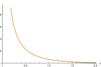
Figure 3: $\cosh y/\sinh y$ (blue) and its approximation (yellow), in practice superposed

Since $h(y,v)\stackrel{{\scriptstyle y\to 0}}{{\to}}0$ and $h(y,v)\simeq\frac{(1-v^{2})^{2}}{48}y^{2}+\ldots$, $\varphi_{0}\simeq m^{2}+\displaystyle\frac{1-v^{2}}{4}\hat{k}^{2}+\displaystyle\frac{1}{48}(1-v^{2})^{2}y^{2}+\ldots$, which yields $e^{\displaystyle-t\varphi_{0}}\displaystyle\frac{\cosh eBt}{\sinh eBt}\simeq e^{\displaystyle-t\big{(}m^{2}+\frac{1-v^{2}}{4}\hat{k}^{2}\big{)}}\;\Big{(}\displaystyle\frac{1}{y}+\displaystyle\frac{y}{3}+(1-v^{2})^{2}\displaystyle\frac{k_{\perp}^{2}}{48eB}y^{2}-\displaystyle\frac{y^{3}}{45}+\ldots\Big{)}$. One gets the following contribution to $T_{\mu\nu}^{N_{3}}(\hat{k},B)$:

$$\frac{\alpha}{2\pi}\;2\sqrt{\pi}(-2eB)\;\;\frac{g_{\mu\nu}^{\parallel}\hat{k}_{\parallel}^{2}-\hat{k}_{\mu}^{\parallel}\hat{k}_{\nu}^{\parallel}}{\hat{k}_{\parallel}^{2}}\int_{0}^{t_{0}}\frac{dt}{\sqrt{t}}\int_{-1}^{+1}\frac{dv}{2}\;e^{\displaystyle-t\big{(}m^{2}+\frac{1-v^{2}}{4}\hat{k}^{2}\big{)}}\Big{(}\frac{eBt}{3}+(1-v^{2})^{2}\frac{k_{\perp}^{2}}{48eB}(eBt)^{2}-\frac{(eBt)^{3}}{45}+\ldots\Big{)},$$ (80)

or, equivalently

$$\frac{\alpha}{2\pi}\;2\sqrt{\pi}(-2eB)\;\;\frac{g_{\mu\nu}^{\parallel}\hat{k}_{\parallel}^{2}-\hat{k}_{\mu}^{\parallel}\hat{k}_{\nu}^{\parallel}}{\hat{k}_{\parallel}^{2}}\frac{1}{\sqrt{eB}}\int_{0}^{y_{0}}\frac{dy}{\sqrt{y}}\int_{-1}^{+1}\frac{dv}{2}\;e^{\displaystyle-\frac{y}{eB}\big{(}m^{2}+\frac{1-v^{2}}{4}\hat{k}^{2}\big{)}}\Big{(}\frac{y}{3}+(1-v^{2})^{2}\frac{k_{\perp}^{2}}{48eB}y^{2}-\frac{y^{3}}{45}+\ldots\Big{)}.$$ (81)

Since, in this last expression, we work at small $y$, it is legitimate to expand the exponential. The leading terms of the integrand are $\frac{y}{3}-\displaystyle\frac{y^{3}}{45}+\ldots$, with additional terms damped by $eB$ factors. So, one gets contributions $\propto\sqrt{eB},\displaystyle\frac{1}{\sqrt{eB}},\ldots$ $\times$ powers of $y_{0}$ (which is $\leq 1$), which, as we shall see, are non-leading.

$\bullet$ For $t\in[t_{0},\infty]$ we consider $\cosh y/\sinh y\approx 1$ and the 2nd contribution to $T_{\mu\nu}$ writes accordingly

$$\frac{\alpha}{2\pi}\;2\sqrt{\pi}(-2eB)\;\;\frac{g_{\mu\nu}^{\parallel}\hat{k}_{\parallel}^{2}-\hat{k}_{\mu}^{\parallel}\hat{k}_{\nu}^{\parallel}}{\hat{k}_{\parallel}^{2}}\frac{1}{\sqrt{eB}}\int_{y_{0}}^{\infty}\frac{dy}{\sqrt{y}}\int_{-1}^{+1}\frac{dv}{2}\;e^{\displaystyle-\frac{y}{eB}\big{(}m^{2}+\frac{1-v^{2}}{4}\hat{k}^{2}\big{)}}\Big{(}e^{\displaystyle\frac{y}{eB}k_{\perp}^{2}h(y,v)}-\frac{1}{y}\Big{)},$$ (82)

or, equivalently

$$\frac{\alpha}{2\pi}\;2\sqrt{\pi}(-2eB)\;\;\frac{g_{\mu\nu}^{\parallel}\hat{k}_{\parallel}^{2}-\hat{k}_{\mu}^{\parallel}\hat{k}_{\nu}^{\parallel}}{\hat{k}_{\parallel}^{2}}\frac{1}{\sqrt{eB}}\int_{y_{0}}^{\infty}\frac{dy}{\sqrt{y}}\int_{-1}^{+1}\frac{dv}{2}\;e^{\displaystyle-\frac{y}{eB}\big{(}m^{2}+\frac{1-v^{2}}{4}\hat{k}_{\parallel}^{2}-k_{\perp}^{2}g(y,v)\big{)}}-e^{\displaystyle-\frac{y}{eB}\big{(}m^{2}+\frac{1-v^{2}}{4}\hat{k}^{2}\big{)}}\frac{1}{y}.$$ (83)

*  First contribution to (83) (main term at $y>y_{0}$)

One needs an approximation of $e^{\frac{y}{eB}k_{\perp}^{2}g(y,v)}$ for $y\geq y_{0}$, which is the most hazardous part. The function $g(y,v)$ has been defined in (70):

$$g(y,v)\equiv\frac{\cosh yv-\cosh y}{2y\sinh y}\approx\frac{e^{yv}-e^{y}}{2ye^{y}}=\frac{1}{2y}\big{(}e^{-y(1-v)}-1\big{)}.$$ (84)

I plot in Figure 4 $g(y,v)\;(blue),-\displaystyle\frac{1}{2y}\;(yellow),\big{(}1-e^{-y(1-v)}\big{)}/2y\;(green)$ at $v=1/20$ (left) and $v=1/2$ (right)

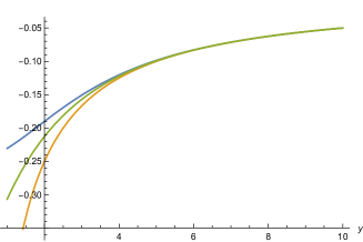
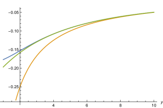
Figure 4: $g(y,v)$ (blue), $-1/2y$ (yellow), $(1-e^{-y(1-v)})/2y$ (yellow), at $v=1/20$ (left) and $v=1/2$ (right)

We notice that $|g|<\displaystyle\frac{1}{2y}$ and $g<0$, therefore $e^{\displaystyle y\frac{k_{\perp}^{2}}{eB}g}\equiv e^{\displaystyle-y\frac{k_{\perp}^{2}}{eB}|g|}>e^{\displaystyle-\frac{k_{\perp}^{2}}{2eB}}$.

By replacing $e^{\displaystyle y\frac{k_{\perp}^{2}}{eB}g}$ by $e^{\displaystyle-\frac{k_{\perp}^{2}}{2eB}}$ we therefore get a lower bound to the (modulus of the) contribution of the main term

$$-T_{\mu\nu}\geq\frac{\alpha}{2\pi}\;2\sqrt{\pi}(2eB)\;\;\frac{g_{\mu\nu}^{\parallel}\hat{k}_{\parallel}^{2}-\hat{k}_{\mu}^{\parallel}\hat{k}_{\nu}^{\parallel}}{\hat{k}_{\parallel}^{2}}\frac{1}{\sqrt{eB}}\int_{y_{0}}^{\infty}\frac{dy}{\sqrt{y}}\int_{-1}^{+1}\frac{dv}{2}\;e^{\displaystyle-\frac{k_{\perp}^{2}}{2eB}}\;e^{\displaystyle-\frac{y}{eB}\big{(}m^{2}+\frac{1-v^{2}}{4}\hat{k}_{\parallel}^{2}\big{)}}.$$ (85)

The exponential under scrutiny is $e^{\displaystyle-\frac{k_{\perp}^{2}}{2eB}\frac{\cosh y-\cosh yv}{\sinh y}}$ and we have used that it is $>e^{\displaystyle-\frac{k_{\perp}^{2}}{2eB}}$. On the other side $\displaystyle\frac{\cosh y-\cosh yv}{\sinh y}>0$ such that $e^{\displaystyle-\frac{k_{\perp}^{2}}{2eB}\frac{\cosh y-\cosh yv}{\sinh y}}<1$. At large $eB$, the upper and lower bounds are very close such that our approximation is expected to be quite accurate.

I now use

$$\int_{y_{0}}^{\infty}dy\;\frac{e^{\displaystyle-by}}{\sqrt{y}}=\sqrt{\frac{\pi}{b}}\;Erf[\sqrt{by}]\Big{|}_{y_{0}}^{\infty},\quad b=\frac{1}{eB}\Big{(}m^{2}+\frac{1-v^{2}}{4}(-k_{0}^{2})\Big{)},$$ (86)

since $Erf[\infty]=1$, it yields

$$\sqrt{\frac{\pi}{b}}\big{(}1-Erf[\sqrt{by_{0}}]\big{)}.$$ (87)

Furthermore, when $x\to 0$, $Erf[x]\sim\displaystyle\frac{2x}{\sqrt{\pi}}$, which is the case since $b$ is very small at $B$ large, such that the result becomes

$$\approx\sqrt{\frac{\pi}{b}}\Big{(}1-\frac{2\sqrt{by_{0}}}{\sqrt{\pi}}\Big{)}=\sqrt{\frac{\pi}{b}}-2\sqrt{y_{0}},$$ (88)

of which the leading contribution is the 1st one, since $b\propto 1/eB$.

* Second contribution to (83) (counterterm at $y>y_{0}$)

$$\int_{y_{0}}^{\infty}dy\;y\frac{e^{\displaystyle-cy}}{y^{3/2}}=-\frac{2e^{-cy}}{\sqrt{y}}-2\sqrt{\pi c}\;Erf[\sqrt{cy}]\Big{|}_{y_{0}}^{\infty},\ c=\frac{1}{eB}\big{(}m^{2}+\frac{1-v^{2}}{4}\hat{k}^{2}\big{)},$$ (89)

which gives

$$\frac{2e^{-cy_{0}}}{\sqrt{y_{0}}}-2\sqrt{\pi c}(1-Erf[\sqrt{cy_{0}}]).$$ (90)

When $c,cy_{0}\to 0$, this can be approximated by $\displaystyle\frac{2(1-cy_{0})}{\sqrt{y_{0}}}-2\sqrt{\pi c}\big{(}1-\displaystyle\frac{2\sqrt{cy_{0}}}{\sqrt{\pi}}\big{)}=\displaystyle\frac{2}{\sqrt{y_{0}}}-2c\sqrt{y_{0}}-2\sqrt{\pi c}+4c\sqrt{y_{0}}=\displaystyle\frac{2}{\sqrt{y_{0}}}+2c\sqrt{y_{0}}-2\sqrt{\pi c}$, which are all sub-leading with respect to the first contribution.

$\bullet$ I shall therefore approximate $T_{\mu\nu}^{N_{3}}$ by its main term at $y>y_{0}$

$$\begin{split}&-T_{\mu\nu}^{N_{3}}(\hat{k},B)\geq\frac{\alpha}{2\pi}2\sqrt{\pi}\;\frac{g_{\mu\nu}^{\parallel}\hat{k}_{\parallel}^{2}-\hat{k}_{\mu}^{\parallel}\hat{k}_{\nu}^{\parallel}}{\hat{k}_{\parallel}^{2}}\frac{(2eB)}{\sqrt{eB}}e^{\displaystyle-\frac{k_{\perp}^{2}}{2eB}}\int_{-1}^{+1}\frac{dv}{2}\;\frac{\sqrt{\pi eB}}{\sqrt{m^{2}-k_{0}^{2}\frac{1-v^{2}}{4}}}\cr&=\alpha(-2eB)e^{\displaystyle-\frac{k_{\perp}^{2}}{2eB}}\;\frac{g_{\mu\nu}^{\parallel}\hat{k}_{\parallel}^{2}-\hat{k}_{\mu}^{\parallel}\hat{k}_{\nu}^{\parallel}}{\hat{k}_{\parallel}^{2}}\int_{-1}^{+1}\frac{dv}{2}\;\frac{1}{\sqrt{m^{2}-k_{0}^{2}\displaystyle\frac{1-v^{2}}{4}}},\end{split}$$ (91)

that is,

$$-T_{\mu\nu}^{N_{3}}(\hat{k},B)\geq\alpha\;(2eB)\;e^{\displaystyle-\frac{k_{\perp}^{2}}{2eB}}\;\;\frac{g_{\mu\nu}^{\parallel}\hat{k}_{\parallel}^{2}-\hat{k}_{\mu}^{\parallel}\hat{k}_{\nu}^{\parallel}}{\hat{k}_{\parallel}^{2}}\frac{1}{k_{0}}\ln\frac{2m+k_{0}}{2m-k_{0}},$$ (92)

and one must remember that the sign $\geq$ is, in practice, an equality.

4.2.3 Summing the contributions

The $N_{3}$ term cancels the logarithmic contribution of the $N_{1}$ part, and one gets

$$T_{\mu\nu}(\hat{k},B\to\infty)\simeq-8\alpha\;m\;g_{\mu 3}g_{\nu 3}\frac{eB}{4m^{2}-k_{0}^{2}}.$$ (93)

The limit $m\to 0$ gives, using (28)

$$\Pi_{\mu\nu}(k,B\to\infty)\stackrel{{\scriptstyle m\to 0}}{{\to}}0.$$ (94)

such that radiative corrections to the photon propagator get frozen at 1-loop when $B\to\infty$.

The cancellation of the logarithmic term ensures in particular that the imaginary part of $\Pi_{\mu\nu}$ vanishes. Its presence would correspond to the creation of $e^{+}e^{-}$ pairs, in contradiction to the property that an external magnetic field cannot transfer energy to a charged particle and cannot trigger such a pair creation (see for example p.83 of [7]).

5 The scalar potential

It does not depend on the choice of counterterms, which are $\propto g_{\mu 3}g_{\nu 3}$ (see sections 4 and 6).

5.1 A reminder

See for example [13].

The electromagnetic 4-vector potential produced by the 4-current $j_{\nu}(y)$ is

$$A_{\mu}(x)=-i\int d^{4}y\;\Delta_{\mu\nu}(x-y)\;j_{\nu}(y).$$ (95)

The current of a pointlike charge $q$ placed at $\vec{y}=0$ is

$$j_{\nu}(y)=q\,\delta_{\nu 0}\,\delta^{3}(\vec{y}).$$ (96)

Therefore

$$\begin{split}A_{\mu}(x)&=-iq\int_{-\infty}^{+\infty}dy_{0}\;\Delta_{\mu 0}(x_{0}-y_{0},\vec{x})\cr&=-iq\int_{-\infty}^{+\infty}dy_{0}\;\Delta_{\mu 0}(x_{0}+y_{0},\vec{x})\cr&=-iq\int_{-\infty}^{+\infty}dy_{0}\;\Delta_{\mu 0}(y_{0},\vec{x}).\end{split}$$ (97)

The usual Coulomb potential is easily recovered when one takes the photon propagator in the Feynman gauge $\Delta_{\mu\nu}\sim-i\displaystyle\frac{g_{\mu\nu}}{(x-y)^{2}}$. Only $A_{0}$ subsists

$$A_{0}(x)\sim-iq\int dy_{0}\;\frac{-i}{y_{0}^{2}-\vec{x}^{2}}\sim\frac{q}{|\vec{x}|}.$$ (98)

In general, in Fourier space

$$\Delta_{\mu\nu}(x)=\frac{1}{(2\pi)^{4}}\int d^{4}k\;e^{ikx}\;\Delta_{\mu\nu}(k),$$ (99)

such that

$$\begin{split}A_{\mu}(x)&=-i\frac{q}{(2\pi)^{4}}\int dy_{0}\,d^{4}k\;e^{i(-k_{0}y_{0}+\vec{k}\vec{x})}\;\Delta_{\mu 0}(k)\cr&=-i\frac{q}{(2\pi)^{4}}\int d^{4}k\;(2\pi)\delta(k_{0})];e^{i(-k_{0}y_{0}+\vec{k}\vec{x})}\;\Delta_{\mu 0}(k)\cr&=-i\frac{q}{(2\pi)^{3}}\int d^{3}k\;e^{i\vec{k}\vec{x}}\;\Delta_{\mu 0}(k_{0}=0,\vec{k}).\end{split}$$ (100)

We see that $k_{0}$ has to be set to $0$ for a static charge.

If we are interested in the scalar potential $A_{0}$

$$\Phi(\vec{x})\equiv A_{0}(\vec{x})=-i\frac{q}{(2\pi)^{3}}\int d^{3}k\;e^{i\vec{k}\vec{x}}\;\Delta_{00}(k_{0}=0,\vec{k}).$$ (101)

So, the geometric series of 1-loop vacuum polarizations that needs to be resummed is that corresponding to $\Delta_{00}(k_{0}=0,\vec{k})$, which involves $\Pi_{00}((k_{0}=0,\vec{k}),B)$

$$\begin{split}\Phi(\vec{k},B)&=-ie[\Delta_{00}(k_{0}=0,\vec{k})]+(-ie)[\Delta_{00}(k_{0}=0,\vec{k})(i\Pi_{00}((k_{0}=0,\vec{k}),B)\Delta_{00}(k_{0}=0,\vec{k})]+\ldots\cr&=(-ie)\frac{\Delta_{00}(k_{0}=0,\vec{k})}{1-i\Pi_{00}((k_{0}=0,\vec{k}),B)\Delta_{00}(k_{0}=0,\vec{k})}\stackrel{{\scriptstyle Feynman\ gauge}}{{=}}\frac{e}{\vec{k}^{2}+\Pi_{00}((k_{0}=0,\vec{k}),B)}.\end{split}$$ (102)

5.2 Calculating $\boldsymbol{\Pi_{00}((k_{0}=0,\vec{k}),B)}$

Eq. (69) gives

$$\Pi_{00}((k_{0}=0,\vec{k}),B)=-\frac{1}{\pi^{2}}\frac{1-n^{2}}{a}V(n,\theta,\eta,u)\;\frac{\alpha}{2\pi}\frac{2\sqrt{\pi}}{\sqrt{eB}}(-)k_{\perp}^{2}\int_{0}^{\infty}\frac{dy}{\sqrt{y}}\int_{-1}^{+1}\frac{dv}{2}\;e^{-(y/eB)\varphi_{0}}\,N_{0}\ \Bigg{|}_{k_{0}=0},$$ (103)

with

$$\begin{split}\varphi_{0}\big{|}_{k_{0}=0}&=m^{2}-\frac{\cosh yv-\cosh y}{2y\sinh y}\;k_{\perp}^{2},\cr N_{0}&=\frac{y}{\sinh y}\Big{(}\cosh yv-\frac{v\cosh y\,\sinh yv}{\sinh y}\Big{)}.\end{split}$$ (104)

Using (37) yields

$$\begin{split}\Pi_{00}((k_{0}=0,\vec{k}),B)&\stackrel{{\scriptstyle s_{\theta}>1/n}}{{\simeq}}+\frac{\alpha}{\pi^{3/2}}\frac{k_{\perp}^{2}}{\sqrt{eB}}\underbrace{\frac{1-\frac{1-i\cot\theta}{2}e^{-a|\vec{k}|(1+u)(s_{\theta}+ic_{\theta})}-\frac{1+i\cot\theta}{2}e^{a|\vec{k}|(u-1)(s_{\theta}-ic_{\theta})}}{a}}_{\frac{1-n^{2}}{\pi}\frac{V}{a}}\cr&\hskip 142.26378pt\underbrace{\int_{0}^{\infty}\frac{dy}{\sqrt{y}}\int_{-1}^{+1}\frac{dv}{2}\;e^{-(y/eB)\varphi_{0}}\,N_{0}\ \Bigg{|}_{k_{0}=0}}_{L(eB,k_{\perp}^{2})},\end{split}$$ (105)

which is a convergent integral. It vanishes at $\boldsymbol{B\to\infty}$ because $N_{0}\stackrel{{\scriptstyle B\to\infty}}{{\to}}0$.

At the limit $a\to 0$ it simplifies to

$$\Pi_{00}((k_{0}=0,\vec{k}),B)\stackrel{{\scriptstyle s_{\theta}>1/n,a\to 0}}{{\simeq}}+\frac{\alpha}{\pi^{3/2}}\frac{k_{\perp}^{2}}{\sqrt{eB}}\underbrace{\frac{|\vec{k}|}{\sin\theta}}_{\frac{1-n^{2}}{\pi}\frac{V}{a}}\underbrace{\int_{0}^{\infty}\frac{dy}{\sqrt{y}}\int_{-1}^{+1}\frac{dv}{2}\;e^{-(y/eB)\varphi_{0}}\,N_{0}\ \Bigg{|}_{k_{0}=0}}_{L(eB,k_{\perp}^{2})},$$ (106)

with $\varphi_{0}$ and $N_{0}$ given in (64.

In our setup $k_{2}=0$, $\sin\theta=k_{1}/|\vec{k}|$ such that $|\vec{k}|/\sin\theta=(k_{1}^{2}+k_{3}^{2})/k_{1}=|\vec{k}|^{2}/k_{1}=|\vec{k}|^{2}/k_{\perp}$.

5.2.1 The function $\boldsymbol{L(eB,k_{\perp}^{2})}$

$$L(eB,k_{\perp}^{2})=\int_{0}^{\infty}\frac{dy}{\sqrt{y}}\int_{-1}^{+1}\frac{dv}{2}\;e^{\displaystyle-\frac{y}{eB}\big{(}m^{2}-\frac{\cosh yv-\cosh y}{2y\sinh y}\;k_{\perp}^{2}\big{)}}\;\frac{y}{\sinh y}\Big{(}\cosh yv-\frac{v\cosh y\,\sinh yv}{\sinh y}\Big{)}.$$ (107)

In practice, in our setup, $k_{\perp}^{2}=k_{1}^{2}$.

Graphically:
* $f(y,v)=\frac{\cosh yv-\cosh y}{2y\sinh y}\leq 0$, such that, even at $m=0$ the exponential is convergent;
* $0\leq N_{0}(y,v)\leq 1$;
therefore the “singularity $1/\sqrt{y}$ is no problem and $L$ is a convergent integral, even at $m=0$. Let $L^{0}=L|_{m=0}$, such that, at the limit $a\to 0$

$$\Pi_{00}((k_{0}=0,\vec{k}),B=0,m=0)\stackrel{{\scriptstyle s_{\theta}>1/n,a\to 0}}{{\simeq}}+\frac{\alpha}{\pi^{3/2}}\frac{k_{\perp}^{2}}{\sqrt{eB}}\frac{|\vec{k}|}{\sin\theta}L^{0}(\frac{k_{\perp}^{2}}{eB}),$$ (108)

with

$$L^{0}(\frac{k_{\perp}^{2}}{eB})=\int_{0}^{\infty}\frac{dy}{\sqrt{y}}\int_{-1}^{+1}\frac{dv}{2}\;e^{\displaystyle-\frac{k_{\perp}^{2}}{eB}\frac{\cosh y-\cosh yv}{2\sinh y}}\;\frac{y}{\sinh y}\Big{(}\cosh yv-\frac{v\cosh y\,\sinh yv}{\sinh y}\Big{)}.$$ (109)

In Figure 5, $L^{0}(x)$ is plotted for $x\in[0,100]$ on the left, while on the right is plotted $xL^{0}(x^{2})$ which will occur when calculating the scalar potential.

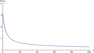
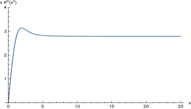
Figure 5: $L^{0}(x)$ (left) and $xL^{0}(x^{2})$ (right).

5.2.2 General expression for the scalar potential $\boldsymbol{\Phi(\vec{x},B)}$ at $\boldsymbol{m\to 0}$ and $\boldsymbol{a\to 0}$

Combining (102) and (108) yields, in Fourier space, to

$$\begin{split}\Phi(\vec{x},B)\stackrel{{\scriptstyle a\to 0,m=0}}{{=}}e\int\frac{d^{3}\vec{k}}{(2\pi)^{3}}\;e^{i\vec{k}\vec{x}}\;\frac{1}{\vec{k}^{2}+\Pi_{00}((k_{0}=0,\vec{k}),B,m=0)}&=e\int\frac{d^{3}\vec{k}}{(2\pi)^{3}}\;e^{i\vec{k}\vec{x}}\;\frac{1}{\vec{k}^{2}+\frac{\alpha}{\pi^{3/2}}\frac{k_{\perp}^{2}}{\sqrt{eB}}\frac{|\vec{k}|}{\sin\theta}L^{0}(\frac{k_{\perp}^{2}}{eB})}\Big{|}_{k_{0}=0}\cr&=e\int\frac{d^{3}\vec{k}}{(2\pi)^{3}}\;e^{i\vec{k}\vec{x}}\;\frac{1}{(k_{3}^{2}+k_{\perp}^{2})\big{(}1++\frac{\alpha}{\pi^{3/2}}\frac{k_{\perp}}{\sqrt{eB}}L^{0}(\frac{k_{\perp}^{2}}{eB})\big{)}},\end{split}$$ (110)

where, in the last line, we have used the characteristics of our setup, $\sin\theta=\frac{k_{1}}{|\vec{k}|}=\frac{k_{\perp}}{|\vec{k}|}$.

5.3 The scalar potential at $\boldsymbol{eB=0}$

Using (76) at $k_{0}=0$

$$T^{00}(\hat{k},B=0)\stackrel{{\scriptstyle m-0}}{{=}}\alpha\frac{\pi}{2}(-k_{\perp}^{2})\frac{1}{\sqrt{\hat{k}^{2}}}\stackrel{{\scriptstyle k_{0}=0}}{{\to}}-\frac{\alpha\pi}{2}k_{\perp}$$ (111)

and taking the limit at $a\to 0$ of $\frac{1-n^{2}}{\pi}\frac{V}{a}$ at $k_{0}=0$ given in (38) yields for $\Pi^{00}$ obtained from (28)

$$\Pi^{00}((0,\vec{k}),B=0)\stackrel{{\scriptstyle a=0,m=0}}{{=}}-\frac{1}{\pi^{2}}\underbrace{(-)\frac{\alpha\pi}{2}k_{\perp}}_{T^{00}}\underbrace{\frac{\pi|\vec{k}|}{\sin\theta}}_{\frac{1-n^{2}}{a}V}=\frac{\alpha}{2}(k_{\perp}^{2}+k_{3}^{2}),$$ (112)

in which we have used again $\sin\theta=k_{1}/|\vec{k}|=k_{\perp}/|\vec{k}|$. One gets accordingly

$$\Phi(\vec{x},B=0)\stackrel{{\scriptstyle a=0,m=0}}{{=}}e\int\frac{d^{3}\vec{k}}{(2\pi)^{3}}\;e^{i\vec{k}\vec{x}}\frac{1}{k_{3}^{2}+k_{\perp}^{2}+\frac{\alpha}{2}(k_{\perp}^{2}+k_{3}^{2})}=\frac{e}{1+\frac{\alpha}{2}}\int\frac{d^{3}\vec{k}}{(2\pi)^{3}}\;e^{i\vec{k}\vec{x}}\frac{1}{|\vec{k}|^{2}},$$ (113)

which is the Coulomb potential renormalized by $\frac{1}{1+\frac{\alpha}{2}}$.

Therefore, even in the absence of external $B$, the Coulomb potential gets renormalized for a graphene-like medium.

This effect results from a subtle interplay between $T_{00}$, in which the peculiarities of the graphene hamiltonian play a major role and which does not vanish at $B=0$, and the “geometric” transmittance $V/a$, which, in particular, does not vanish at $a\to 0$. The screening effect, small at $\alpha=1/137$, can become important in a strongly coupled medium $\alpha\sim 1$.

5.4 The scalar potential at $\boldsymbol{B\to\infty}$

Because of the factor $1/\sqrt{eB}$ and of the decrease of $L^{0}$ at large $B$ (see Figure 5) that occur in $\Pi^{00}$ (see (108)), $\Pi_{00}\stackrel{{\scriptstyle eB\to\infty}}{{\to}}0$, such that

$$\Phi(\vec{x},B=\infty)=e\int\frac{d^{3}k}{(2\pi)^{3}}\;e^{i\vec{k}\vec{x}}\;\frac{1}{\vec{k}^{2}},$$ (114)

which is the Coulomb potential.

This is due in particular to the property that $\Pi_{00}$ is subleading at $B\to\infty$ (the leading $\Pi_{33}$ grows instead with $B$, but does not influence the scalar potential of a static charge).

5.5 The scalar potential for $\boldsymbol{eB\not=0}$

I use cylindrical coordinates: $d^{3}\vec{k}=k_{\perp}dk_{\perp}d\omega dk_{3}$ with $\omega\in[0,2\pi]$. In our setup $k_{1}=k_{\perp}$ up to the sign, which is accounted for by $\omega\in[0,2\pi]$. So, we can write (110) as

$$\Phi(\vec{x},B)=\frac{e}{(2\pi)^{3}}\int_{0}^{2\pi}d\omega\int dk_{3}\int_{0}^{\infty}dk_{\perp}\;k_{\perp}e^{i(k_{3}z+k_{\perp}x_{\perp}\cos\omega)}\frac{1}{(k_{3}^{2}+k_{\perp}^{2})\big{(}1+\frac{\alpha}{\pi^{3/2}}\frac{k_{\perp}}{\sqrt{eB}}L^{0}(\frac{k_{\perp}^{2}}{eB})\big{)}}.$$ (115)

5.5.1 Potential along $\boldsymbol{z}$

I consider (115) at $x_{\perp}=0$

$$\begin{split}\Phi(z,B)&=\frac{e}{(2\pi)^{3}}\int_{0}^{2\pi}d\omega\int dk_{3}\int_{0}^{\infty}dk_{\perp}\;k_{\perp}e^{ik_{3}z}\frac{1}{(k_{3}^{2}+k_{\perp}^{2})\big{(}1+\frac{\alpha}{\pi^{3/2}}\frac{k_{\perp}}{\sqrt{eB}}L^{0}(\frac{k_{\perp}^{2}}{eB})\big{)}}\cr&=\frac{e}{4\pi^{2}}\int dk_{3}\int_{0}^{\infty}dk_{\perp}\;k_{\perp}e^{ik_{3}z}\frac{1}{(k_{3}^{2}+k_{\perp}^{2})\big{(}1+\frac{\alpha}{\pi^{3/2}}\frac{k_{\perp}}{\sqrt{eB}}L^{0}(\frac{k_{\perp}^{2}}{eB})\big{)}}.\end{split}$$ (116)

$\int dk_{3}\;\frac{e^{ik_{3}z}}{k_{3}^{2}+c^{2}}=\frac{\pi}{c}\;e^{-cz},z>0\Rightarrow$

$$\Phi(z,B)=\frac{e}{4\pi^{2}}\int_{0}^{\infty}dk_{\perp}\;k_{\perp}\frac{1}{1+\frac{\alpha}{\pi^{3/2}}\frac{k_{\perp}}{\sqrt{eB}}L^{0}(\frac{k_{\perp}^{2}}{eB})}\;\frac{\pi}{c}\;e^{-cz},\quad c^{2}=k_{\perp}^{2}.$$ (117)

It gives

$$\Phi(z,B)=\frac{e}{4\pi}\int_{0}^{\infty}dk_{\perp}\frac{e^{-zk_{\perp}}}{1+\frac{\alpha}{\pi^{3/2}}\frac{k_{\perp}}{\sqrt{eB}}L^{0}(\frac{k_{\perp}^{2}}{eB})}.$$ (118)

If one neglects all corrections proportional to $\alpha$, one gets $\Phi(z)\to\frac{e}{4\pi}\int_{0}^{\infty}dk_{\perp}e^{-zk_{\perp}}=\frac{e}{4\pi z}$ which is the Coulomb potential.

Going to the integration variable $u=k_{\perp}/\sqrt{eB}$, $\Phi(z,B)$ rewrites

$$\Phi(z,B)=\frac{e}{4\pi z}z\sqrt{eB}\int_{0}^{\infty}du\;\frac{e^{-z\sqrt{eB}u}}{1+\frac{\alpha}{\pi^{3/2}}\;u\,L^{0}(u^{2})}=\frac{e}{4\pi z}\;z\sqrt{eB}\;F(z\sqrt{eB}),$$ (119)

in which $z\sqrt{eB}\;F(z\sqrt{eB})$ gives the correction to the Coulomb potential. This correction is plotted on Figure 6 for $\alpha=1/137$ (left) and $\alpha=1/2$ (right).

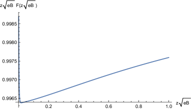
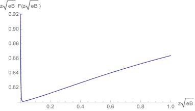
Figure 6: the scalar potential along $z$ at the limit $a\to 0$. On the left $\alpha=1/137$, on the right $\alpha=1/2$.

The curves should not be trusted at $z\sqrt{eB}\to 0$. Indeed, the limit $eB\to 0$ should be taken before changing to the integration variable to $y=ieBs$ (see subsection 3.3), which goes to $0$ with $B$. This has been done in subsection 4.1, with the consequences explicitly studied in subsection 5.3. The quasi-straight lines of Figure 6 should be continued till they cross the vertical axes at $\frac{1}{1+1/2\times 137}\approx.996$ and $\frac{1}{1+1/4}\approx.8$. In particular, the singularity of the potential at $z=0$ is not canceled, only renormalized.

The scalar potential going to Coulomb at $B\to\infty$, and the curves of Figure 6 go asymptotically to $1$.

5.5.2 Potential at $\boldsymbol{z=0}$ in the transverse plane

Setting $z=0$ in (110) yields

$$\begin{split}\Phi(x_{\perp},B)&=e\int\frac{d^{3}\vec{k}}{(2\pi)^{3}}\;e^{i\vec{k}_{\perp}\vec{x}_{\perp}}\;\frac{1}{\vec{k}^{2}+\Pi_{00}(0,\vec{k})}\cr&=e\int\frac{d^{3}\vec{k}}{(2\pi)^{3}}\;e^{i\vec{k}_{\perp}\vec{x}_{\perp}}\;\frac{1}{(k_{\perp}^{2}+k_{3}^{2})\big{(}1+\frac{\alpha}{\pi^{3/2}}\frac{k_{\perp}}{\sqrt{eB}}L^{0}(\frac{k_{\perp}^{2}}{eB})\big{)}}.\end{split}$$ (120)

In cylindrical coordinates as before, $d^{3}\vec{k}=dk_{3}\;k_{\perp}dk_{\perp}\;d\omega$ such that

$$\Phi(x_{\perp},B)=\frac{e}{(2\pi)^{3}}\int dk_{3}\int_{0}^{\infty}dk_{\perp}\;k_{\perp}\int_{0}^{2\pi}d\omega\;e^{ik_{\perp}x_{\perp}\cos\omega}\frac{1}{(k_{\perp}^{2}+k_{3}^{2})\big{(}1+\frac{\alpha}{\pi^{3/2}}\frac{k_{\perp}}{\sqrt{eB}}L^{0}(\frac{k_{\perp}^{2}}{eB})\big{)}}.$$ (121)

Integrating $\int d\omega$ yields

$$\begin{split}\Phi(x_{\perp},B)&=\frac{e}{4\pi^{2}}\int dk_{3}\int_{0}^{\infty}dk_{\perp}\;k_{\perp}\frac{J_{0}(k_{\perp}x_{\perp})}{(k_{3}^{2}+k_{\perp}^{2})(1+\frac{\alpha}{\pi^{3/2}}\frac{k_{\perp}}{\sqrt{eB}}L^{0}(\frac{k_{\perp}^{2}}{eB}))}\cr&=\frac{e}{4\pi^{2}}\int_{0}^{\infty}dk_{\perp}\;k_{\perp}\frac{J_{0}(k_{\perp}x_{\perp})}{1+\frac{\alpha}{\pi^{3/2}}\frac{k_{\perp}}{\sqrt{eB}}L^{0}(\frac{k_{\perp}^{2}}{eB})}\;\frac{\pi}{k_{\perp}}\cr&=\frac{e}{4\pi}\int_{0}^{\infty}dk_{\perp}\;\frac{J_{0}(k_{\perp}x_{\perp})}{1+\frac{\alpha}{\pi^{3/2}}\frac{k_{\perp}}{\sqrt{eB}}L^{0}(\frac{k_{\perp}^{2}}{eB})},\end{split}$$ (122)

where $J_{0}$ stands for the Bessel function of 1st kind. I cast $\Phi(x_{\perp},B)$ in the form

$$\begin{split}\Phi(x_{\perp},B)&=\frac{e}{4\pi x_{\perp}}\;x_{\perp}\sqrt{eB}\int_{0}^{\infty}\frac{dk_{\perp}}{\sqrt{eB}}\frac{J_{0}(\frac{k_{\perp}}{\sqrt{eB}}\;x_{\perp}\sqrt{eB})}{1+\frac{\alpha}{\pi^{3/2}}\frac{k_{\perp}}{\sqrt{eB}}\;L^{0}(\frac{k_{\perp}^{2}}{eB})}\cr&=\frac{e}{4\pi x_{\perp}}\;x_{\perp}\sqrt{eB}\ G(x_{\perp}\sqrt{eB}),\quad G(x_{\perp}\sqrt{eB})=\int_{0}^{\infty}du\;\frac{J_{0}(x_{\perp}\sqrt{eB}\,u)}{1+\frac{\alpha}{\pi^{3/2}}\,u\;L^{0}(u^{2})},\end{split}$$ (123)

in which we have gone to the variable $u=k_{\perp}/\sqrt{eB}$. With respect to the scalar potential along the $z$ axis and formula (119), the decreasing $\exp[-z\sqrt{eB}\,u]$ has been replaced with the oscillating and decreasing $J_{0}(x_{\perp}\sqrt{eB}\,u)$.

If one neglects the corrections proportional to $\alpha$ one gets $\Phi(x_{\perp})\approx\frac{e}{4\pi x_{\perp}}\int_{0}^{\infty}dk_{\perp}x_{\perp}J_{0}(k_{\perp}x_{\perp})=\frac{e}{4\pi x_{\perp}}\times 1$, which is the Coulomb potential.

Since getting curves for the potential turns out to be very difficult, let us only understand why the deviations from Coulomb are in general very small. The corrections to $1$ in the denominator of (123) are $\frac{\alpha}{\pi^{3/2}}uL^{0}(u^{2})\approx\frac{\alpha}{5.57}uL^{0}(u^{2})$. We have seen on Figure 5 that $uK^{0}(u^{2})\leq 3$ which makes this correction $\leq.54\,\alpha$. One accordingly expects sizable corrections to the Coulomb potential only in strongly coupled systems. Like before, at $z\sqrt{eB}=0$, $\Phi(x_{\perp})=\frac{Coulomb}{1+\alpha/2}$.

6 Alternative choices of counterterms

6.1 Boundary terms and counterterms

Counterterms are devised to fulfill suitable renormalization conditions (in our case the on mass-shell conditions (67)), and in particular cancel unwanted infinities. In standard QED₃₊₁ in external $B$, this is enough to ensure the $(3+1)$-transversality of the vacuum polarization $k_{\mu}k_{\nu}\Pi^{\mu\nu}=0$ (see for example [5]), closely connected to gauge invariance and to the conservation of the electromagnetic current. However, as shown in [7] (see p.70 for example), this is obtained by including inside the counterterms the boundary terms of partial integrations. Since boundary terms obviously depend on the external $B$ (and have no reason to be transverse), the property that the sum [boundary terms + counterterms] do not depend on $B$ actually means that the raw counterterms do depend on it. This is non-standard (see for example [14]), but one presumably cannot state whether this is legitimate or not; along the path followed by Schwinger and [7], one is induced to consider that introducing $B$-dependent counterterms can be necessary. I therefore propose below to improve the situation concerning the transversality of $\Pi_{\mu\nu}$ along this line.

The counterterms should eventually be adapted:
* to fulfill of course the renormalization conditions (67);
* to cure the divergence of the so-called $B_{\mu\nu}$ of subsection 3.1 coming from classically imposing $p_{3}=0$ and $p_{3}-k_{3}=0$ for internal electron propagators to match a graphene-like Hamiltonian;
* to eventually achieve full $3+1$-transversality $k_{\mu}k_{\nu}\Pi^{\mu\nu}=0$ instead of restricted $2+1$-transversality $\hat{k}_{\mu}\hat{k}_{\nu}T_{\mu\nu}=0=\hat{k}_{\mu}\hat{k}_{\nu}\Pi^{\mu\nu}$.

In addition, the production of $e^{+}e^{-}$ pairs should not occur in the sole presence of a constant external $B$, which sets constraints on the imaginary part of $\Pi_{\mu\nu}$.

As we have seen in subsection 3.4

$$\hat{k}_{\mu}\hat{k}_{\nu}T^{\mu\nu}(\hat{k},B)=0\Rightarrow k_{\mu}k_{\nu}\Pi^{\mu\nu}=\frac{1}{\pi^{2}}\frac{1-n^{2}}{a}k_{3}^{2}\;V(n,\theta,\eta,u)\;T_{33}(\hat{k},B),$$ (124)

such that the non-transversality of $\Pi^{\mu\nu}$ is solely connected to $T^{33}$. This is why we shall only consider modifying the counterterms in relation with $T^{33}$.

I shall investigate the two following subtractions, the first being independent on $B$, the second depending on $B$:
* $T_{\mu\nu}^{ren}(\hat{k}B)=T_{\mu\nu}^{bare}(\hat{k},B)-g_{\mu 3}g_{\nu 3}\,T_{33}^{bare}|_{B=0}$ ;
* $T_{\mu\nu}^{ren}(\hat{k}B)=T_{\mu\nu}^{bare}(\hat{k},B)-g_{\mu 3}g_{\nu 3}\,T_{33}^{bare}$.

In both cases only the indices $\mu=3,\nu=3$ are concerned, such that $T_{00}=T_{00}^{bare}$, and therefore $\Pi_{00}$, stay unchanged, together with the scalar potential. The study of their limits at $k_{0}=0$ and $m=0$ is as done in section 5.

One can only rely here on transversality to select the counterterms. However, modifying $\Pi_{33}$ has consequences on other physical quantities, like the refractive index (see for example the beginning of [12]). It may happen that reasonable results for the refractive index (and/or agreement with experiments) can only be achieved at the price of giving up $3+1$-transversality, leaving only the restricted $2+1$-transversality. Then, deeper investigations should be done to understand what “gauge invariance” truly means for such a medium as graphene. I leave this for further works.

6.2 $\boldsymbol{B}$-independent counterterm. $\boldsymbol{\Pi_{\mu\nu}}$ made $\boldsymbol{(3+1)}$-transverse only at $\boldsymbol{B=0}$, non-vanishing at $\boldsymbol{B=0}$ and at $\boldsymbol{B=\infty}$

$$T_{33}^{bare}(\hat{k},B)=\frac{\alpha}{2\pi}\,2\sqrt{\pi}\int_{0}^{\infty}\frac{dt}{\sqrt{t}}\int_{-1}^{+1}\frac{dv}{2}\;e^{-t\varphi_{0}}\;\Big{[}(N_{0}-N_{1})\hat{k}_{\parallel}^{2}+N_{0}k_{\perp}^{2}\underbrace{-2eB\;\frac{\cosh eBt}{\sinh eBt}}_{\to divergence\ at\ t=0}\Big{]}$$ (125)

always depends on $B$, and

$$T_{33}^{bare}(\hat{k},B=0)=\frac{\alpha}{2\pi}\,2\sqrt{\pi}\int_{0}^{\infty}\frac{dt}{\sqrt{t}}\int_{-1}^{+1}\frac{dv}{2}\;e^{-t\big{(}m^{2}+\frac{1-v^{2}}{4}\hat{k}^{2}\big{)}}\;\Big{[}(1-v^{2})\hat{k}^{2}-\frac{2}{t}\Big{]}.$$ (126)

$T_{33}^{bare}$ is divergent at $t\to 0$.

One considers ($\varphi_{0},N_{0},N_{1},N_{2}$ are given in (64))

$$\begin{split}T_{\mu\nu}(\hat{k},B)&=T_{\mu\nu}^{bare}(\hat{k},B)-g_{\mu 3}g_{\nu 3}\,T_{33}^{bare}(\hat{k},B=0)=\frac{\alpha}{2\pi}\;2\sqrt{\pi}\int_{0}^{\infty}\frac{dt}{\sqrt{t}}\int_{-1}^{+1}\frac{dv}{2}\cr&e^{\displaystyle-t\varphi_{0}}\Bigg{[}N_{0}[g_{\mu\nu}\hat{k}^{2}-\hat{k}_{\mu}\hat{k}_{\nu}]-N_{1}[\underbrace{g_{\mu\nu}^{\parallel}\hat{k}_{\parallel}^{2}-\hat{k}_{\mu}^{\parallel}\hat{k}_{\nu}^{\parallel}}_{\hat{k}_{\parallel}^{2}g_{\mu 3}g_{\nu 3}}]+N_{2}[g_{\mu\nu}^{\perp}\hat{k}_{\perp}^{2}-\hat{k}_{\mu}^{\perp}\hat{k}_{\nu}^{\perp}]-2\frac{eB\cosh eBt}{\sinh eBt}\;\underbrace{\frac{g_{\mu\nu}^{\parallel}\hat{k}_{\parallel}^{2}-\hat{k}_{\mu}^{\parallel}\hat{k}_{\nu}^{\parallel}}{\hat{k}_{\parallel}^{2}}}_{\equiv g_{\mu 3}g_{\nu 3}}\Bigg{]}\cr&-\underbrace{\frac{g_{\mu\nu}^{\parallel}\hat{k}_{\parallel}^{2}-\hat{k}_{\mu}^{\parallel}\hat{k}_{\nu}^{\parallel}}{\hat{k}_{\parallel}^{2}}}_{\equiv g_{\mu 3}g_{\nu 3}}\;e^{\displaystyle-t\big{(}m^{2}+\frac{1-v^{2}}{4}\hat{k}^{2}\big{)}}\;\Big{[}\underbrace{(1-v^{2})\hat{k}^{2}}_{new/section\,\ref{section:renorm1}}\underbrace{-\frac{2}{t}}_{cancels\;divergence\;at\;t=0}\Big{]}.\end{split}$$ (127)

So doing, the corresponding $\Pi_{\mu\nu}$:
* vanishes at $k^{2}=0$ thanks to $(1-n^{2})V$, in particular at $B=0$: the renormalization condition are therefore satisfied;
* does not vanish in general at $B=0$;
* is finite thanks to the term $\propto 2/t$ in the counterterms;
* is transverse at $B=0$, $k^{\mu}k^{\nu}\Pi_{\mu\nu}|_{B=0}=0$, but it is so only at $B=0$.

Unlike in subsection 4.2 it does not vanish at $B\to\infty$.

6.2.1 At $\boldsymbol{B=0}$

Only $T_{33}$ vanishes at $B=0$ because, then, $N_{0}\to 1-v^{2},N_{1}\to 0,N_{2}\to 0,\varphi_{0}\to m^{2}+\frac{1-v^{2}}{4}\;\hat{k}^{2}$; one has

$$\begin{split}T_{\mu\nu}(\hat{k},B=0)&=T_{\mu\nu}^{bare}(\hat{k},B=0)-g_{\mu 3}g_{\nu 3}\,T_{33}^{bare}|_{B=0}=\frac{\alpha}{2\pi}\;2\sqrt{\pi}\int_{0}^{\infty}\frac{dt}{\sqrt{t}}\int_{-1}^{+1}\frac{dv}{2}\cr&e^{\displaystyle-t\big{(}m^{2}+\frac{1-v^{2}}{4}\hat{k}^{2}\big{)}}\;(1-v^{2})\Big{[}\underbrace{(g_{\mu\nu}\hat{k}^{2}-\hat{k}_{\mu}\hat{k}_{\nu})-g_{\mu 3}g_{\nu 3}\;\hat{k}^{2}}_{\hat{g}_{\mu\nu}\hat{k}^{2}-\hat{k}_{\mu}\hat{k}_{\nu}}\Big{]},\end{split}$$ (128)

which is transverse because $k^{\mu}k^{\nu}(\hat{g}_{\mu\nu}\hat{k}^{2}-\hat{k}_{\mu}\hat{k}_{\nu})\equiv\hat{k}^{\mu}\hat{k}^{\nu}(\hat{g}_{\mu\nu}\hat{k}^{2}-\hat{k}_{\mu}\hat{k}_{\nu})=0$. One gets

$$\begin{split}T_{\mu\nu}(\hat{k},B=0)&=\alpha(\hat{g}_{\mu\nu}\hat{k}^{2}-\hat{k}_{\mu}\hat{k}_{\nu})\int_{-1}^{+1}\frac{dv}{2}\;\frac{1-v^{2}}{\sqrt{m^{2}+\frac{1-v^{2}}{4}\hat{k}^{2}}}\cr&=\alpha(\hat{g}_{\mu\nu}\hat{k}^{2}-\hat{k}_{\mu}\hat{k}_{\nu})\frac{2}{\sqrt{\hat{k}^{2}}}\;\frac{1}{2}\Big{(}\frac{2m}{\sqrt{\hat{k}^{2}}}+\big{(}1-\frac{4m^{2}}{\hat{k}^{2}}\big{)}\cot^{-1}\frac{2m}{\sqrt{\hat{k}^{2}}}\Big{)}.\end{split}$$ (129)

The limit $m\to 0$ is the transverse

$$T_{\mu\nu}(\hat{k},B=0,m=0)=\frac{\pi\;\alpha}{2}\;\frac{\hat{g}_{\mu\nu}\hat{k}^{2}-\hat{k}_{\mu}\hat{k}_{\nu}}{\sqrt{\hat{k}^{2}}}.$$ (130)

6.2.2 At $\boldsymbol{B=\infty}$

$N_{0},N_{2}\stackrel{{\scriptstyle B\to\infty}}{{\to}}0,N_{1}\stackrel{{\scriptstyle B\to\infty}}{{\to}}-y(1-v^{2})$.

$$T_{\mu\nu}(\hat{k},B=\infty)=T_{\mu\nu}^{bare}(\hat{k},B=\infty)-g_{\mu 3}g_{\nu 3}\,T_{33}^{bare}|_{B=0},$$ (131)

such that

$$\begin{split}T_{\mu\nu}(\hat{k},B\to\infty)&=T_{\mu\nu}^{bare}(\hat{k},B\to\infty)-g_{\mu 3}g_{\nu 3}\,T_{33}^{bare}|_{B=0}=\frac{\alpha}{2\pi}\;2\sqrt{\pi}\int_{0}^{\infty}\frac{dt}{\sqrt{t}}\int_{-1}^{+1}\frac{dv}{2}\cr&e^{\displaystyle-t\varphi_{0}}\Bigg{[}+y(1-v^{2})[g_{\mu\nu}^{\parallel}\hat{k}_{\parallel}^{2}-\hat{k}_{\mu}^{\parallel}\hat{k}_{\nu}^{\parallel}]-2g_{\mu 3}g_{\nu 3}\;\frac{eB\cosh eBt}{\sinh eBt}\;\Bigg{]}\cr&\hskip 56.9055pt-g_{\mu 3}g_{\nu 3}\;e^{\displaystyle-t\big{(}m^{2}+\frac{1-v^{2}}{4}\hat{k}^{2}\big{)}}\;\Big{[}(1-v^{2})\hat{k}^{2}-\frac{2}{t}\Big{]},\end{split}$$ (132)

which is non-transverse as expected. It is what we have already calculated in subsection 4.2 to which is added
$S\equiv\frac{\alpha}{2\pi}\;2\sqrt{\pi}\int_{0}^{\infty}\frac{dt}{\sqrt{t}}\int_{-1}^{+1}\frac{dv}{2}(-)g_{\mu 3}g_{\nu 3}\;e^{\displaystyle-t\big{(}m^{2}+\frac{1-v^{2}}{4}\hat{k}^{2}\big{)}}\;(1-v^{2})\hat{k}^{2}$.

$$\begin{split}S&=-\frac{\alpha}{2\pi}\;2\sqrt{\pi}\;\hat{k}^{2}\;g_{\mu 3}g_{\nu 3}\int_{0}^{\infty}\frac{dt}{\sqrt{t}}\int_{-1}^{+1}\frac{dv}{2}\;(1-v^{2})\;e^{\displaystyle-t\big{(}m^{2}+\frac{1-v^{2}}{4}\hat{k}^{2}\big{)}}\cr&=-\alpha\;\hat{k}^{2}\;g_{\mu 3}g_{\nu 3}\int_{-1}^{+1}\frac{dv}{2}\;\frac{1-v^{2}}{\sqrt{m^{2}+\frac{1-v^{2}}{4}\hat{k}^{2}}}\cr&=-\alpha\;\hat{k}^{2}\;g_{\mu 3}g_{\nu 3}\;\frac{2}{\sqrt{\hat{k}^{2}}}\;\frac{1}{2}\Big{(}\frac{2m}{\sqrt{\hat{k}^{2}}}+\big{(}1-\frac{4m^{2}}{\hat{k}^{2}}\big{)}\cot^{-1}\frac{2m}{\sqrt{\hat{k}^{2}}}\Big{)}\cr&=-\alpha\;g_{\mu 3}g_{\nu 3}\sqrt{\hat{k}^{2}}\Big{(}\frac{2m}{\sqrt{\hat{k}^{2}}}+\big{(}1-\frac{4m^{2}}{\hat{k}^{2}}\big{)}\cot^{-1}\frac{2m}{\sqrt{\hat{k}^{2}}}\Big{)}.\end{split}$$ (133)

One gets accordingly, at the limit $m\to 0$, the non-transverse

$$T_{\mu\nu}(\hat{k},B\to\infty)\stackrel{{\scriptstyle m\to 0}}{{\to}}-\alpha\;\frac{\pi}{2}\;g_{\mu 3}g_{\nu 3}\;\sqrt{\hat{k}^{2}}$$ (134)

which, unlike in subsection 4.2, does not vanish at $m=0$.

6.3 $\boldsymbol{B}$-dependent counterterm. $\boldsymbol{\Pi^{\mu\nu}}$ made always $\boldsymbol{(3+1)}$-transverse, non-vanishing at $\boldsymbol{B=0}$, vanishing at $\boldsymbol{B=\infty}$

To make $T_{\mu\nu}(\hat{k},B)$, and therefore also $\Pi_{\mu\nu}(k,B)$ always $(3+1)$- transverse, one drastically subtracts $g_{\mu 3}g_{\nu 3}\,T_{33}(\hat{k},B)$ from $T_{\mu\nu}^{bare}(\hat{k},B)$ (this also cancels the divergence). One then gets

$$\begin{split}T_{\mu\nu}(\hat{k},B)=T_{\mu\nu}^{bare}(\hat{k},B)-g_{\mu 3}g_{\nu 3}\,T_{33}^{bare}(\hat{k},B)&=\frac{\alpha}{2\pi}\;2\sqrt{\pi}\int_{0}^{\infty}\frac{dt}{\sqrt{t}}\int_{-1}^{+1}\frac{dv}{2}\cr&\hskip-142.26378pte^{-t\varphi_{0}}\;\Bigg{[}N_{0}\Big{(}\underbrace{(g_{\mu\nu}\hat{k}^{2}-\hat{k}_{\mu}\hat{k}_{\nu})-\hat{k}^{2}g_{\mu 3}g_{\nu 3}}_{\equiv\hat{g}_{\mu\nu}\hat{k}^{2}-\hat{k}_{\mu}\hat{k}_{\nu}}\Big{)}-N_{1}\Big{(}\underbrace{(g_{\mu\nu}^{\parallel}\hat{k}_{\parallel}^{2}-\hat{k}_{\mu}^{\parallel}\hat{k}_{\mu}^{\parallel})-\hat{k}_{\parallel}^{2}g_{\mu 3}g_{\nu 3}}_{=0}\Big{)}+N_{2}\big{(}g_{\mu\nu}^{\perp}k_{\perp}^{2}-k_{\mu}^{\perp}k_{\nu}^{\perp}\big{)}\Bigg{]},\end{split}$$ (135)

in which $\varphi_{0},N_{0},N_{2}$ are as usual given in (64).

6.3.1 At $\boldsymbol{B=0}$

The result is of course the same transverse result as in subsection 6.2.1.

6.3.2 At $\boldsymbol{B=\infty}$

$N_{0},N_{2}\to 0$ such that $T_{\mu\nu}(\hat{k},B=\infty)=0$: the 1-loop vacuum polarization vanishes at $B\to\infty$ such that quantum corrections to the photon propagator get frozen at this order.

Unlike in subsection 4.2, the limit $m\to 0$ is not necessary to achieve the vanishing of $\Pi_{\mu\nu}$ at $B\to\infty$.

7 Salient features of the calculation, remarks and conclusion

7.1 Generalities

The calculation that we have performed has two main characteristics:
* it accounts for all Landau levels of the internal electrons;
* it simulates a graphene-like medium of very small thickness $2a$, inside which the interactions between photons and electrons are localized (at 1-loop); this technique, which was shown in the case of the electron self-energy, to reproduce the results of reduced QED₃₊₁ on a 2-brane, has still more important consequences for the vacuum polarization (in which the external photon is not constrained to propagate inside the medium) with the occurrence of a transmittance function. The latter plays a crucial role, in particular to implement on mass-shell renormalization conditions. No singularity occurs when $a\to 0$, and our calculations of the scalar potential have been mostly done at this simple limit .

7.2 Dimensional reduction

The widely spread belief [15] that reduced QED₃₊₁ on a 2-brane provides a fair description of graphene has been comforted in [8] concerning the propagation of an electron; however, in view of the present results, one can hardly believe that it provides a reliable treatment of the photon propagation at 1-loop because it skips the transmittance and cannot allow for suitable renormalization conditions. In particular spurious divergences at $m=0$, due to inappropriate counterterms, are likely to arise, in addition to the divergence of $\frac{1-n^{2}}{a}T^{\mu\nu}$ at $a\to 0$ which is no longer canceled by the transmittance $V$. $T_{\mu\nu}$ is the part of $\Pi_{\mu\nu}$ that has the closest properties to reduced QED₃₊₁ on a 2 brane (in there no “effective” internal photon propagator gets involved). It is however very far from giving a suitable description of the vacuum polarization of the graphene-like medium under consideration.

One of the motivations for this work was also to study the competing roles of two types of dimensional reduction. The first is the equivalence, when $B\to\infty$, of QED₃₊₁ with QED₁₊₁ with no $B$ (Schwinger model). It was an essential ingredient for example in [16] [17], where the screening of the Coulomb potential due to a superstrong $B$ in QED₃₊₁ was investigated. The second is the “confinement” of electrons inside the $(x,y)$ plane for a very thin graphene-like medium. Which of the two spatial subspaces, the $z$ axis (along $B$) or the $(x,y)$ plane of the medium, would win and control the underlying physics was not clear a priori.

We have seen that, as far as the vacuum polarization is concerned, only $\Pi_{33}$ survives at the limit $B\to\infty$ (like becoming $(0+1)$-dimensional). It can even vanish when $m\to 0$, depending on the choice of counterterms. When it does, radiative corrections to the photon propagator get frozen at 1-loop when $B\to\infty$.

7.3 Radiative corrections to the Coulomb potential

The scalar potential is controlled by $\Pi_{00}$ which is non-leading at large $B$ (with the same caveat as above in the case where $\Pi_{33}$ vanishes). As a consequence, its modification by the external $B$ is completely different from what happens in standard QED₃₊₁ (see for example [16] [17]).

The limit of an infinitely thin graphene-like medium exhibits an intrinsic renormalization of the Coulomb potential by $1/(1+\alpha/2)$ at $B=0$. Going to stronger $B$ tends instead to restore the genuine Coulomb potential. The interpolation between $B=0$ and $B=\infty$ being smooth, the scalar potential can substantially deviate from Coulomb only in a strongly coupled medium and for weak or vanishing magnetic fields.

7.4 Conclusion and prospects

Basic principles of Quantum Field Theory provide a clean approach to radiative corrections for a graphene-like medium in external $B$. We have exhibited once more (see [8] [9]) the primordial importance of the renormalization conditions and of the counterterms.

Many aspects remain to be investigated. Let us mention:
* how does the scalar potential depend on the thickness $a$ when it is taken non-vanishing?
* can there be experimental tests of, for example, the renormalization of the Coulomb potential and of its non-trivial dependence on $B$?
* how are the optical properties of graphene, which in particular depend on $\Pi_{33}$, modified at 1-loop by the external $B$?
* can this, or other physical properties or constraints, help fixing the counterterms?
* can $(3+1)$-transversality and gauge invariance be achieved or should one accommodate with “reduced” $(2+1)$-transversality? Which type of gauge invariance is then at play, which electromagnetic current is / is not conserved?
* is it justified to introduce $B$-dependent counterterms? Do other examples act in favor of it?
* how does dressing the photon propagator modifies the electron self-energy? can consistent resummations be achieved, while implementing at each order suitable renormalization conditions? what comes out for the electron mass? does a gap always open in graphene like we witnessed at 1-loop with a bare photon?

All these we postpone to forthcoming works.

Aknowledgments: very warm thanks are due to Olivier Coquand who has been a main contributor to section 2, and to Mikail Vysotsky for contunuous exchanges.

Appendix A Demonstration of eq. (10)

I start from (5), in which, now, the fermion propagator $G$ depends on $B$. The notations are always $v=(v_{0},v_{1},v_{2},v_{3})=(\hat{v},v_{3}),\hat{v}=(v_{0},v_{1},v_{2})$.

$$\begin{split}\Delta^{\rho\sigma}(x,y)&=e^{2}\int d^{3}\hat{u}\int_{-a}^{+a}du_{3}\int d^{3}\hat{v}\int_{-a}^{+a}dv_{3}\cr&\int\frac{d^{4}k}{(2\pi)^{4}}\;e^{ik(u-x)}\Delta^{\rho\mu}(k)\,\gamma_{\mu}\int\frac{d^{4}p}{(2\pi)^{4}}\;e^{ip(u-v)}G(\hat{p},B)\,\gamma_{\nu}\int\frac{d^{4}r}{(2\pi)^{4}}\;e^{ir(v-u)}G(\hat{r},B)\int\frac{d^{4}s}{(2\pi)^{4}}\;e^{is(y-v)}\Delta^{\sigma\nu}(s)\cr&=e^{2}\int d^{3}\hat{u}\int_{-a}^{+a}du_{3}\int d^{3}\hat{v}\int_{-a}^{+a}dv_{3}\;\int\frac{d^{3}\hat{k}}{(2\pi)^{3}}\frac{dk_{3}}{2\pi}\;e^{i\hat{k}(\hat{u}-\hat{x})}e^{ik_{3}(u_{3}-x_{3})}\Delta^{\rho\mu}(k)\cr&\hskip 42.67912pt\gamma_{\mu}\int\frac{d^{3}\hat{p}}{(2\pi)^{3}}\,\frac{dp_{3}}{2\pi}\;e^{i\hat{p}(\hat{u}-\hat{v})}e^{ip_{3}(u_{3}-v_{3})}G(\hat{p},B)\,\gamma_{\nu}\int\frac{d^{3}\hat{r}}{(2\pi)^{3}}\,\frac{dr_{3}}{2\pi}\;e^{i\hat{r}(\hat{v}-\hat{u})}e^{ir_{3}(v_{3}-u_{3})}G(\hat{r},B)\cr&\hskip 42.67912pt\int\frac{d^{3}\hat{s}}{(2\pi)^{3}}\,\frac{ds_{3}}{2\pi}\;e^{i\hat{s}(\hat{y}-\hat{v})}e^{is_{3}(y_{3}-v_{3})}\Delta^{\sigma\nu}(s)\cr&=e^{2}\underbrace{\int d^{3}\hat{u}\;e^{i\hat{u}(\hat{k}+\hat{p}-\hat{r})}}_{(2\pi)^{3}\delta(\hat{p}+\hat{k}-\hat{r})}\int d^{3}\hat{v}\;e^{i\hat{v}(-\hat{p}+\hat{r}-\hat{s})}\int_{-a}^{+a}du_{3}\int_{-a}^{+a}dv_{3}\;\int\frac{d^{3}\hat{k}}{(2\pi)^{3}}\,\frac{dk_{3}}{2\pi}\;e^{i\hat{k}(-\hat{x})}e^{iq_{3}(u_{3}-x_{3})}\Delta^{\rho\mu}(k)\cr&\hskip 42.67912pt\gamma_{\mu}\int\frac{d^{3}\hat{p}}{(2\pi)^{3}}\,\frac{dp_{3}}{2\pi}\;e^{ip_{3}(u_{3}-v_{3})}G(\hat{p},B)\,\gamma_{\nu}\int\frac{d^{3}\hat{r}}{(2\pi)^{3}}\,\frac{dr_{3}}{2\pi}\;e^{ir_{3}(v_{3}-u_{3})}G(\hat{r},B)\cr&\hskip 42.67912pt\int\frac{d^{3}\hat{s}}{(2\pi)^{3}}\,\frac{ds_{3}}{2\pi}\;e^{i\hat{s}(\hat{y})}e^{is_{3}(y_{3}-v_{3})}\Delta^{\sigma\nu}(s)\cr&=e^{2}\underbrace{\int d^{3}\hat{v}\;e^{i\hat{v}(\hat{k}-\hat{s})}}_{(2\pi)^{3}\delta(\hat{k}-\hat{s})}\int_{-a}^{+a}du_{3}\int_{-a}^{+a}dv_{3}\;\int\frac{d^{3}\hat{k}}{(2\pi)^{3}}\,\frac{dk_{3}}{2\pi}\;e^{i\hat{k}(-\hat{x})}e^{ik_{3}(u_{3}-x_{3})}\Delta^{\rho\mu}(k)\cr&\hskip 42.67912pt\gamma_{\mu}\int\frac{d^{3}\hat{p}}{(2\pi)^{3}}\,\frac{dp_{3}}{2\pi}\;e^{ip_{3}(u_{3}-v_{3})}G(\hat{p},B)\,\gamma_{\nu}\int\frac{dr_{3}}{2\pi}\;e^{ir_{3}(v_{3}-u_{3})}G(\hat{p}+\hat{k},B)\cr&\hskip 42.67912pt\int\frac{d^{3}\hat{s}}{(2\pi)^{3}}\,\frac{ds_{3}}{2\pi}\;e^{i\hat{s}(\hat{y})}e^{is_{3}(y_{3}-v_{3})}\Delta^{\sigma\nu}(s)\cr&=e^{2}\int_{-a}^{+a}du_{3}\int_{-a}^{+a}dv_{3}\;\int\frac{d^{3}\hat{k}}{(2\pi)^{3}}\,\frac{dk_{3}}{2\pi}\;e^{i\hat{k}(-\hat{x})}e^{ik_{3}(u_{3}-x_{3})}\Delta^{\rho\mu}(\hat{k},k_{3})\cr&\hskip 42.67912pt\gamma_{\mu}\int\frac{d^{3}\hat{p}}{(2\pi)^{3}}\,\frac{dp_{3}}{2\pi}\;e^{ip_{3}(u_{3}-v_{3})}G(\hat{p},B)\,\gamma_{\nu}\int\frac{dr_{3}}{2\pi}\;e^{ir_{3}(v_{3}-u_{3})}G(\hat{p}+\hat{k},B)\int\frac{ds_{3}}{2\pi}\;e^{i\hat{k}(\hat{y})}e^{is_{3}(y_{3}-v_{3})}\Delta^{\sigma\nu}(\hat{k},s_{3})\cr&=e^{2}\int\frac{dr_{3}}{2\pi}\int\frac{ds_{3}}{2\pi}\int_{-a}^{+a}du_{3}\;e^{iu_{3}(k_{3}+p_{3}-r_{3})}\int_{-a}^{+a}dv_{3}\;e^{iv_{3}(-p_{3}+r_{3}-s_{3})}\cr&\hskip 28.45274pt\int\frac{d^{3}\hat{k}}{(2\pi)^{3}}\,\frac{dk_{3}}{2\pi}\;e^{i\hat{k}(-\hat{x})}e^{ik_{3}(-x_{3})}\Delta^{\rho\mu}(\hat{k},k_{3})\,\gamma_{\mu}\int\frac{d^{3}\hat{p}}{(2\pi)^{3}}\,\frac{dp_{3}}{2\pi}\;G(\hat{p},B)\,\gamma_{\nu}\,G(\hat{p}+\hat{k},B)e^{i\hat{k}(\hat{y})}e^{is_{3}(y_{3})}\Delta^{\sigma\nu}(\hat{k},s_{3})\cr&=\int\frac{dp_{3}}{2\pi}\int\frac{dk_{3}}{2\pi}\int\frac{dr_{3}}{2\pi}\int\frac{ds_{3}}{2\pi}\int_{-a}^{+a}du_{3}\;e^{iu_{3}(k_{3}+p_{3}-r_{3})}\int_{-a}^{+a}dv_{3}\;e^{iv_{3}(-p_{3}+r_{3}-s_{3})}\cr&\hskip 42.67912pt\int\frac{d^{3}\hat{k}}{(2\pi)^{3}}\;e^{i\hat{k}(\hat{y}-\hat{x})}e^{ik_{3}(-x_{3})}e^{is_{3}(y_{3})}\Delta^{\rho\mu}(\hat{k},k_{3})\Delta^{\sigma\nu}(\hat{k},s_{3})\ \underbrace{e^{2}\int\frac{d^{3}\hat{p}}{(2\pi)^{3}}\;\gamma_{\mu}\,G(\hat{p},B)\,\gamma_{\nu}\,G(\hat{p}+\hat{k},B)}_{iT_{\mu\nu}(\hat{k},B)},\end{split}$$ (136)

which is eq. (10).

References

- [1]
- [2]
- [3] M.O. GOERBIG: “Electronic properties of graphene in a strong magnetic field”, Rev. Mod. Phys. 83 (2011) 1193.
- [4] J. SCHWINGER: “Quantum Electrodynamics. II. Vacuum Polarization and Self-Energy”, Phys. Rev. 75 (1949) 651.
- [5] J. SCHWINGER: “On Gauge Invariance and Vacuum Polarization”, Phys. Rev. 82 (1951) 664.
- [6] W.Y. TSAI: Vacuum polarization in homogeneous magnetic fields”, Phys. Rev. D 10 (1974) 2699.
- [7] W. DITTRICH, M. REUTER: “Effective Lagrangians in Quantum Electrodynamics”, Springer-Verlag, Lecture Notes in Physics 220 (1985).
- [8] B. MACHET: “Non-vanishing at of the 1-loop self-mass of an electron of mass propagating in a graphene-like medium in a constant external magnetic field”, arXiv:1607.00838 [hep-ph].
- [9] B. MACHET: “The 1-loop self-energy of an electron in a strong external magnetic field revisited”, arXiv:1510.03244 [hep-ph], Int. J. Mod. Phys. A 31 (2016) 1650071.
- [10] E.V. GORBAR, V.P. GUSYNIN & V.A. MIRANSKY: “Dynamical chiral symmetry breaking on a brane in reduced QED”, Phys. Rev. D 64, 105028 (2001).
- [11] M. Sh. PEVZNER & D.V. KHOLOD: “Static potential of a point charge in reduced ”, Russian Physics Journal, Vol.52, n0 10 (2009) 1077.
- [12] O. COQUAND & B. MACHET: “Refractive properties of graphene in a medium-strong external magnetic field”, arXiv:1410.6585 [hep-ph].
- [13] A.E. SHABAD & V.V. USOV: “Electric field of a pointlike charge in a strong magnetic field and ground state of a hydrogenlike atom”, Phys. Rev. D 77, 025001 (2008).
- [14] J. COLLINS: “Renormalization”, Cambridge monographs on mathematical physics (2004)
- [15] E.V. GORBAR, V.P. GUSYNIN, V.A. MIRANSKY & I.A. SHOVKOVY: “Magnetic field driven metal-insulator phase transition in planar systems”. Phys. Rev. B 66, 045108 (2002).
- [16] M.I. VYSOTSKY: “Atomic levels in superstrong magnetic fields and QED of massive electrons: screening”, Pis’ma v ZhETF 92 (2010) 22-26.
- [17] B. MACHET & M.I. VYSOTSKY: “Modification of Coulomb law and energy levels of the hydrogen atom in a superstrong magnetic field”, arXiv:1011.1762 [hep-ph], Phys. Rev. D 83, 025022 (2011)
- [18]