Discovery of a Perseus-like cloud in the early Universe

We present the discovery of a molecular cloud at $z_{\rm abs}\approx 2.5255$ along the line of sight to the quasar SDSS J 000015.17$+$004833.3. We use a high-resolution spectrum obtained with the Ultraviolet and Visual Echelle Spectrograph together with a deep multi-wavelength medium-resolution spectrum obtained with X-Shooter (both on the Very Large Telescope) to perform a detailed analysis of the absorption lines from ionic, neutral atomic and molecular species in different excitation levels, as well as the broad-band dust extinction.
We find that the absorber classifies as a Damped Lyman-$\alpha$ system (DLA) with $\log N({H\textsc{i}})({\rm cm}^{-2})=20.8\pm 0.1$. The DLA has super-Solar metallicity ($Z\sim 2.5Z_{\odot}$, albeit with factor 2-3 uncertainty) with a depletion pattern typical of cold gas and an overall molecular fraction $f=2N($H₂)/($2N$(H${}_{2})+N({H\textsc{i}}))\sim 50$%. This is the highest $f$-value observed to date in a high-$z$ intervening system. Most of the molecular hydrogen arises from a clearly identified narrow ($b\sim$0.7 ${\rm km\,s^{-1}}$), cold component in which carbon monoxide molecules are also found, with $\log N($CO$)\approx 15$. With the help of the spectral synthesis code Cloudy, we study the chemical and physical conditions in the cold gas. We find that the line of sight probes the gas deep after the H i-to-H₂ transition in a $\sim$4-5 pc-size cloud with volumic density $n_{\rm H}\sim$ 80 cm^-3 and temperature of only 50 K. Our model suggests that the presence of small dust grains (down to about 0.001 ${\rm\mu m}$) and high cosmic ray ionisation rate ($\zeta_{\rm H}\sim$ a few times $10^{-15}$ s^-1) are needed to explain the observed atomic and molecular abundances. The presence of small grains is also in agreement with the observed steep extinction curve that also features a 2175 Å bump.
Interestingly, the chemical and physical properties of this cloud are very similar to what is seen in diffuse molecular regions of the nearby Perseus complex, despite the former being observed when the Universe was only 2.5 Gyr old. The high excitation temperature of CO rotational levels towards J0000$+$0048 betrays however the higher temperature of the cosmic microwave background. Using the derived physical conditions, we correct for a small contribution (0.3 K) of collisional excitation and obtain $T_{\rm CMB}(z=2.53)\approx 9.6$ K, in perfect agreement with the predicted adiabatic cooling of the Universe.

1 Introduction

The formation and evolution of galaxies is strongly dependent on the physical properties of the gas in and around galaxies. Indeed, the gas is the reservoir of baryons from which stars form and at the same time, it integrates the chemical and physical outputs from star-formation activity. The gas that is accreted onto galaxies has to cool down and go through different transitional processes that will determine its properties during its evolution before the final collapse that give birth to stars. Different phases are indeed identified in the interstellar medium, depending on the temperature and density and whether the matter is ionised or neutral (atomic or molecular). In their two-phase model, Field et al. (1969) showed that thermal equilibrium leads neutral gas to segregate into a dense phase, the cold neutral medium (CNM), embedded into a diffuse intercloud phase, the warm neutral medium (WNM). Detailed theoretical and numerical works (e.g. Krumholz et al., 2009; Sternberg et al., 2014) show that a transition from H i to H₂ then occurs in the former phase, depending on the balance between H₂ formation on the surface of dust grains (e.g. Jura, 1974b), and its dissociation by UV photons (e.g. Dalgarno & Stephens, 1970), itself dependent on both self- and dust-shielding.

Observationally, UV absorption spectroscopy of Galactic clouds towards nearby stars revealed that the molecular fraction, $f=2$H${}_{2}/(2$H${}_{2}+{H\textsc{i}})$, sharply increases above a H i column density threshold of 5$\times 10^{20}\leavevmode\nobreak\ {\rm cm}^{-2}$. A similar threshold has been found by Reach et al. (1994) from far-infrared emission studies of interstellar clouds, using dust as a tracer for H₂. Higher column-density thresholds were observed in the Magellanic Clouds (Tumlinson et al., 2007), which could be the consequence of a higher UV radiation field together with a lower metallicity in these environments. However, it is also possible that a significant fraction of the observed H i column density is actually unrelated to the atomic envelopes of the H₂-absorbing clouds (Welty et al., 2012), since $N({H\textsc{i}})$ was derived through unresolved 21-cm emission, while $N($H${}_{2})$ was measured in absorption.

This highlights the main difficulty in observing the transition regions: because molecular clouds have sizes of only a few tens to a few hundred parsec (e.g. Fukui & Kawamura, 2010) it is very difficult to compare H₂ with its associated H i in the cloud envelope without also integrating nearby atomic gas. High spatial resolution (sub-pc) studies exist for nearby molecular clouds such as the Perseus cloud. Lee et al. (2012) observed relatively uniform H i surface density of $\Sigma_{\rm HI}\sim 6-8$ M_⊙ pc^-2 around H₂ clouds, in agreement with the theoretical expectations based on H₂ microphysics at Solar metallicity, assuming CNM a priori (Krumholz et al., 2009) or not (Bialy et al., 2015).

Ideally, we would also like to study the atomic to molecular transition and the subsequent star formation over parsec scales in other galaxies. Observations of nearby galaxies have been possible at slightly sub-kpc resolution, revealing a saturation value around $\Sigma_{\rm HI}\approx 9$ M_⊙ pc^-2 (Bigiel et al., 2008). However, the observational techniques applied in the local Universe are not applicable yet in the distant Universe without a further strong loss of spatial resolution. Prescriptions of star-formation over galactic scales, such as the empirical relation between the molecular to atomic ratio and the hydrostatic pressure (e.g. Blitz & Rosolowsky, 2006) are nevertheless available and can be used in evolution models of galaxies (e.g. Lagos et al., 2011), although this corresponds to an extrapolation at high redshift of a phenomenon observed in the local Universe. The increase of sensitivity in sub-mm astromomy has also permited tremendous progress in recent years with detailed studies of the relation between molecular content and star formation at intermediate redshifts (e.g. Tacconi et al., 2013), although still limited to relatively bright and massive galaxies. In addition, observations of atomic gas through H i 21-cm emission (currently limited to $z<0.4$, e.g. Catinella et al. 2008; Freudling et al. 2011; Fernández et al. 2016) will have to await future radio facilities such as the Square Kilometre Array.

At high redshift, information about gas in the Universe can be accurately obtained through absorption studies towards bright background sources. In particular, damped Lyman-$\alpha$ systems (DLAs, see Wolfe et al. 2005 for a review), with $N({H\textsc{i}})\geq 2\times 10^{20}$ ${\rm cm}^{-2}$, trace the neutral gas in a cross-section weighted manner, independently of the luminosity of the associated object. DLAs have been conjectured to be originating from gas associated with galaxies, in particular since DLAs contain the bulk of the neutral gas at high redshift (e.g. Prochaska et al., 2005; Prochaska & Wolfe, 2009; Noterdaeme et al., 2009b, 2012a) and their metallicity is increasing with decreasing redshift (e.g. Rao et al., 2006; Rafelski et al., 2012). While the dust production in the bulk of DLAs seems to be very low (Murphy & Bernet, 2016), the excitation of atomic and molecular species indicate some ongoing star-formation activity (e.g. Wolfe et al., 2004; Srianand et al., 2005; Neeleman et al., 2015). This is also suggested by numerical simulations (e.g. Cen, 2012; Bird et al., 2014) or semi-analytical models (e.g. Berry et al., 2016) but association with galaxies remain difficult to establish directly, with only a few associations between intervening DLAs and galaxies have been revealed so far at $z>2$ (Møller & Warren, 1993; Møller et al., 2004; Fynbo et al., 2010; Krogager et al., 2012; Noterdaeme et al., 2012b; Bouché et al., 2013; Kashikawa et al., 2014; Hartoog et al., 2015; Srianand et al., 2016). Indeed, statistical studies show a low level of in-situ star formation (Rahmani et al., 2010; Fumagalli et al., 2015), although Ly-$\alpha$ emission has been detected through stacking in sub-samples with the highest H i column densities (Noterdaeme et al., 2014), suggesting the latter arise more likely from gas associated with galaxies at small impact parameters.

Noterdaeme et al. (2015a) suggested that H₂ is more frequently found in high column density DLAs, but that the measured overall molecular fraction remains much lower than what would be expected from single clouds, even at the typically low metallicities of DLAs. This indicates that most of the observed H i column density along the line of sight is actually unrelated to the H₂ core and does not participate in its shielding (see also Noterdaeme et al., 2015b). This again marks the difficulty of distinguishing the H i envelope of molecular clouds from unrelated atomic gas along the same line of sight. Several methods have been developped to statistically derive the CNM fraction in DLAs. The low detection rate of 21-cm absorption in DLAs indicates high average spin temperatures and hence that most DLAs are dominated by WNM (e.g. Kanekar et al., 2014). Neeleman et al. (2015) recently suggested that the bulk of neutral gas could be in the CNM for at least 5% of DLAs, based on the fine-structure excitation of singly ionised carbon and silicon. This further indicates that such clouds can be as small as a few parsecs. A small size of CNM clouds is also inferred from the lack of correspondance between 21-cm and H₂ absorption seen in DLAs (Srianand et al., 2012) and by the partial coverage of the background quasar’s broad line region by H₂-bearing clouds (e.g. Balashev et al., 2011).

Because H₂-bearing systems are rare among the overall DLA population (e.g. Ledoux et al., 2003; Noterdaeme et al., 2008; Jorgenson et al., 2014), directly targeting H₂ (instead of blindly targeting H i gas) could provide a more efficient way to study the phase transition. Unfortunately, H₂ lines are located in the ${\rm Ly}\,\alpha$ forest and difficult to detect at low spectral resolution (except when the absorption is in the damped regime, Balashev et al., 2014). In turn, neutral carbon provides an excellent tracer of H₂ molecules (e.g. Snow & McCall, 2006), since the ionisation energy of C i is close to that of H₂ photodissociation. Furthermore, several transitions are located out of the ${\rm Ly}\,\alpha$ forest, making it possible to search for strong C i absorption even at low spectral resolution (see Ledoux et al., 2015). Such selection has led to the first detections of CO molecules in absorption at $z>1.6$, which also opened the exciting possibility to directly measure the cosmic microwave background (CMB) temperature through the excitation of CO (Noterdaeme et al., 2011). In the two high redshift cases where H₂ lines were also covered, we measured overall molecular fractions of about 25% (Srianand et al., 2008; Noterdaeme et al., 2010), i.e. significantly higher than in other H₂-bearing DLAs, that generally have $f\sim 1\%$ or less (Ledoux et al., 2003).

In our quest for molecular-rich systems in the Sloan Digital Sky Survey-III (see Ledoux et al., 2015, for the corresponding search in the SDSS-II), we found a new case, at $z_{\rm abs}\sim 2.5$ towards the quasar SDSS J000015.17$+$004833.3 (hereafter J0000$+$0048) with strong C i absorption and prominent 2175 Å bump that we followed-up with the Very Large Telescope. The characteristics of this system in terms of molecular fraction, CO column density, and metallicity supersede all values measured in DLAs so far. A cold, molecular-bearing component is clearly identified, allowing us to perform an unprecedented detailed analysis of the chemical and physical conditions in the molecular cloud and to study the transition from the atomic to the molecular phase. We present our observations in Sect. 2, the absorption-line analysis of ionic, atomic and molecular species in Sect. 3. We discuss the metallicity and dust abundance in Sect. 4, the extinction in Sect. 5 and the physical conditions in the cloud in Sect. 6. We use CO to measure the cosmic microwave background temperature at $z=2.53$ in Sect. 7. We search for star-formation activity in Sect. 8 and conclude in Sect. 9.

2 Observations and data reduction

2.1 UVES

High-resolution spectroscopic observations of J0000$+$0048 ($z_{\rm em}\approx 3.03$) were carried out using the Ultraviolet and Visual Echelle Spectrograph (UVES; Dekker et al., 2000) mounted on the unit 2 of the 8.2 m very large telescope (VLT) at Paranal observatory under two distinct ESO programmes 093.A-0126(A) in 2014 (P93) and 096.A-0354(A) in 2015 (P96). The former observations were all performed using the standard beam splitter with 390+564 setting at a slit width of $0.9\arcsec$.

The latter (P96) were mostly performed with the same setting but with a narrower slit width of $0.7\arcsec$ in the red arm, and attached Th-Ar calibration. We also observed the quasar 2$\times$4200 s with central wavelength set to 760 nm in the red arm in order to extend the spectral coverage over the redshifted absorption position of useful metal species (Zn ii, Fe ii). These were taken with a $0.9\arcsec$-wide slit. We used a CCD readout with 2$\times$2 binning and set the slit position to paralactic angle for all the observations to minimize the effects of atmospheric dispersion. A summary of the observations is shown in Table 1.

The data were reduced using UVES Common Pipeline Library (CPL) data reduction pipeline release 6.5 using an optimal extraction (Horne, 1986). We use 4^th order polynomials to find the dispersion solution. The individual science exposures were shifted to the heliocentric-vacuum frame correcting for the observatory’s motion towards the line of sight at the exposure mid point, using the air-to-vacuum relation from Ciddor (1996).

All exposures taken with the BLUE arm were obtained using a $0.9^{\prime\prime}$-wide slit and extracted onto a fixed wavelength grid with a pixel step of 2.5 ${\rm km\,s^{-1}}$ that corresponds to the pixel size on the CCD. The spectrum of each echelle order was interpolated onto this global grid so that no further rebinning was required neither when merging orders of an exposure nor when combing different exposures. Similarly, exposures taken with the RED arm have higher resolution and smaller pixel sizes and were extracted on a grid with a pixel step of 2.0 ${\rm km\,s^{-1}}$.

Cosmic ray residuals and bad pixels were flagged using a semi-interactive procedure and the data quality was checked to remove a few failed exposures. Individual 1D extractions were then scaled and combined together into three final 1D spectra: a “blue” spectrum, with spectral resolution 6.30 ${\rm km\,s^{-1}}$; a “red” spectrum with resolution ranging from 5.45 to 5.80 ${\rm km\,s^{-1}}$ corresponding to all exposures taken with $0.9\arcsec$ slit and a higher resolution “red” spectrum, with resolution 4.60-4.70 ${\rm km\,s^{-1}}$, combining the $0.7\arcsec$-wide slit exposures. The average S/N per pixel is about 8 at 4000 Å in the blue spectrum. The combined red spectrum has in turn S/N$\sim$20 at 5300 Å.

2.2 X-Shooter

Deep, medium-resolution spectroscopic observations of J0000$+$0048 over the full wavelength range from $\sim$320 nm to $\sim 2.25$ $\mu$m were carried out at the VLT unit 3 using X-Shooter under ESO programme 096.A-0924(B). We performed all observations using the Nodding mode and slit widths of 1.3″, 0.9″ and 1.2″ for the UVB, VIS and NIR arm, respectively, and a binning of 1$\times$2. We used different slit position angles to maximise the spatial coverage around the quasar location. The log of observations is shown in Table 1.

Our X-Shooter data reduction heavily relies on the pipeline supplied by ESO in its version 2.5.2 (Modigliani et al., 2010). For every position angle, we used the pipeline to apply a flat-field correction, order tracing and rectification of individual frames in each nodding position individually. In the UVB and VIS arm, the sky spectrum was subtracted using regions in the $11\arcsec$-long X-Shooter slit free of signal. In the NIR, the intensity of the sky spectrum is high so we used the frame taken at the alternate nodding position closest in time for background subtraction. Wavelength and flux calibration were performed using arc lamp lines observed during daytime and the nightly spectrophotometric standard, respectively.

This process provided us with sky-subtracted, wavelength- and flux-calibrated 2D spectra. After cosmic-ray and bad-pixel detection using our own algorithm based on Laplacian-filter edge detection, we averaged these frames with variance weighting. This yielded a single frame per arm and position angle. We then obtained the 1D spectra by optimal extraction, where the appropriate weights along the spatial direction were derived using a Moffat-function fitted to the data. Finally, the spectra were corrected for Galactic foreground reddening (Schlafly & Finkbeiner, 2011) and converted into a vacuum heliocentric reference frame. We checked the quality of the flux calibration by comparing the spectra against each other and found agreement within 15% in the UVB (and better in the other arms). We also found no evidence for significant chromatic slit losses in the data by comparing with accurate multi-band photometry (see Sect. 5).

Because X-Shooter sits at the Cassegrain focus of the VLT, shifts in the wavelength solution by about 0.5 Å are not uncommon due to flexure (e.g. Bristow et al., 2011). This is also expected since the observations were performed off the parallactic angle. Thanks to UVES observations of the same object, we indeed noticed and corrected for a wavelength distortion in the UVB arm: We smoothed the UVES spectrum to X-Shooter’s spectral resolution and cross-correlated the resulting spectrum with the X-Shooter data over 200 Å chunks. The wavelength distortion is different for each observation but can be very well approximated by a linear function of the wavelength (see also Chen et al., 2014). We thus corrected for this distortion before combining the individual 1D exposures, improving the wavelength calibration accuracy by a factor of more than 10 compared to the pipeline results (Fig. 1) without losing spectral resolution in the final spectrum due to blurring effect. The combined X-Shooter spectrum has S/N$\sim$ 35, 55 and 25 and resolution around 75, 32 and 35 ${\rm km\,s^{-1}}$ in the UV, visual and near infrared, respectively.

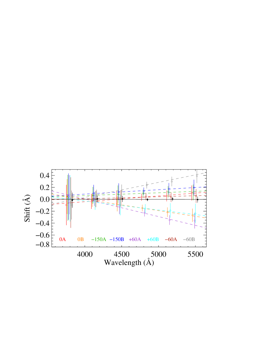
Figure 1: X-Shooter wavelength distortion in the UVB arm for the different exposures. Points with different colours represent averages in 200 Å chunks for different PAs (whose names, given in the bottom, correspond to the angle in degrees East of North, and “A/B” for first/second observation with same PA). The black filled dots correspond to the combined spectrum.

Table 1: Log of observations

Program ID	Setting/Mode	Slit widths	Observing dates	Exposure time
		(arcsec)		(s)
UVES
093.A-0126(A)	390$+$564	0.9, 0.9	Aug 2014	5$\times$4800 s
096.A-0354(A)	390$+$564	0.9, 0.7	Oct-Nov 2015	6$\times$4200 s
096.A-0354(A)	437$+$760	0.9, 0.9	Nov 2015	2$\times$4200 s
X-shooter
096.A-0924(B)	Nodding	1.3, 0.9, 1.2	Sep-Dec 2015, Aug 2016	8$\times$2$\times$(1400, 1430, $3\times$480)

3 Absorption line analysis

We detect metal absorption lines in the $z_{\rm abs}=2.525$ absorption system from various ionisation stages from high-ionisation species (e.g. C iv, Al iii, see Fig. 2) and singly ionised species (Si ii, Ni ii, Zn ii and Fe ii) spread over about 400 ${\rm km\,s^{-1}}$. We detect a narrow component at the extreme red edge of the profile in which we also detect neutral (S i, Mg i, Cl i, C i) and molecular (H₂, CO) species. While the overall kinematic profile is interesting –with a large velocity extent and absorption strengths varying differently with velocity for different ions, suggesting galactic winds– we mostly focus on the molecular component in this paper. We use vpfit (Carswell & Webb, 2014) version 10.3 to model the absorption profiles using multi-component Voigt-profile fitting in order to obtain redshifts, Doppler parameters and column densities of different species.

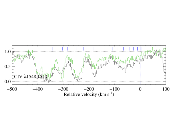
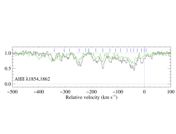
Figure 2: High ionisation species detected towards J0000$+$0048 in the UVES spectrum. The green profile corresponds the reddest transition for each doublet. The ticks marks correspond to the location of singly ionised metal components, and the zero-velocity scale is set at the position of the molecular component. In this, and in all analoguous figures presenting absorption lines, the y-axis shows the normalised flux.

During our analysis, we combine the two red UVES spectra into a single spectrum using an inverse variance weighting. In principle, the resulting spectral point spread function (SPSF) becomes the combination of the two Gaussian SPSF as done by Carswell et al. (2012). In practice, because we are using data from the same instrument with resolutions that differ by only 20%, the resulting SPSF can very well be approximated by a single Gaussian with resolution ranging from 5 to 5.25 ${\rm km\,s^{-1}}$ over the region covered by both original spectra. We checked that fitting both red spectra simultaneously or using their combination provides consistent results and therefore provide here the results using the combined spectrum. For the particular case of CO, we test this more in detail and also provide the simultaneous fit to the two sets of UVES data.

3.1 Atomic hydrogen

We determine the H i column density of the system by simultaneously fitting a Voigt profile to the damped ${\rm Ly}\,\alpha$ absorption line and the continuum of the background quasar. Higher-order Lyman lines are not usable because of blending with stronger damped H₂ lines (see Sect. 3.4). We use the X-Shooter spectrum since it has a much higher signal-to-noise ratio (S/N) than the UVES spectrum in this region, and it is flux calibrated, making easier to determine the continuum placement. We obtain $\log N({H\textsc{i}})=20.8\pm 0.1$. As expected, the UVES data is also consitent with this value, see Fig. 3.

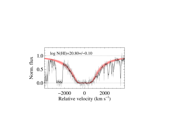
Figure 3: Measurement of the H i column density at $z_{\rm abs}=2.525$. The X-Shooter data is represented in black, while the UVES data, boxcar-smoothed by 5 pixels is represented in grey. The Voigt profile fit is shown in red with the associated uncertainty as a shaded region.

3.2 Metals

About twenty velocity components with a wide dynamical range of optical depths are distinctly identified in the profiles of Si ii and Fe ii thanks to several transitions spanning a range of oscillator strengths. We use these species together with S i (whose 1807 Å transition is blended with Si ii$\lambda$1808) to obtain a first solution for the component structure. We then include Ni ii and Fe ii and let the column densities vary freely while the Doppler parameters and redshifts are tied together for singly ionised species. The redshift and Doppler parameters for neutral species (S i and Mg i) are kept independent.

A very narrow component ($b\approx 0.6\leavevmode\nobreak\ {\rm km\,s^{-1}}$) corresponding to the neutral and molecular species is clearly seen at the extreme red edge of the profiles of Si ii$\lambda$1808 and Zn ii$\lambda\lambda$2026,2062 while much weaker in Fe ii lines and not detected at all in Ni ii (see the component at $v=0$ ${\rm km\,s^{-1}}$in Fig. 4). This already indicates a high level of dust depletion since the later species are refractory while zinc is a volatile element (e.g. Pettini et al., 1997). We use this narrow component ($z=2.52546$) as the reference for the zero-velocity in all figures and discussions in the paper. We also note that we do not make any assumption on the velocity structure (e.g. Doppler parameter) of this component and fit the molecular, atomic, and ionic species independently. The results from fitting the lines are also shown in Fig. 4 and the corresponding parameters provided in Table 2. We measure total column densities of respectively $\log N$(cm^-2) = 15.93$\pm$0.17 (Si ii), 13.99$\pm$0.04 (Ni ii), 14.09$\pm$0.45 (Zn ii) and 15.14$\pm$0.03 (Fe ii). We note that the Zn ii$\lambda$2062 line could be blended with Cr ii absorption (Zn ii$\lambda$2026 as well, but the nearby Cr ii line has very low oscillator strength). However, we do not detect the unblended Cr ii$\lambda\lambda$2056,2066 lines despite strong oscillator strengths. The effect of chromium on the measurement of $N({Zn\textsc{ii}})$ should therefore be largely negligible.

We also detect P ii$\lambda$1532 (P ii$\lambda$1301 is unfortunately lost within the saturated O i$\lambda$1302 profile) in the two strongest components, although close to the noise level. We therefore fixed the redshifts and Doppler parameters to the values determined from other metals and obtain $\log N({P\textsc{ii}})\sim 14.5\pm 0.1$. Finally, S ii lines are detected but redshifted in the ${\rm Ly}\,\alpha$ forest. While two of them ($\lambda\lambda 1250,1253$) are not severely blended, their oscillator strengths are similar. This, and the low signal-to-noise ratio achieved in this region of the UVES spectrum prevent us from getting meaningful constraints through line fitting, in particular for the strong narrow component. However, we checked that the data is consistent with the expected profile assuming a Solar zinc-to-sulphur ratio in the gas phase.

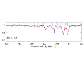
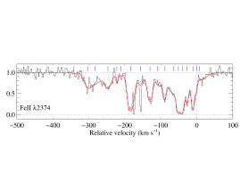
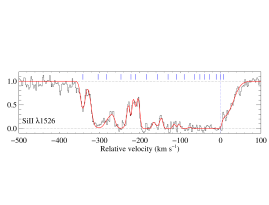
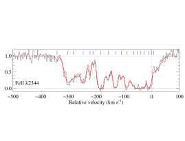
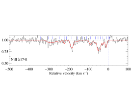
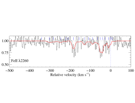
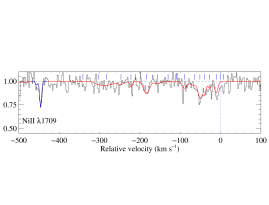
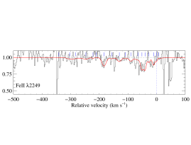
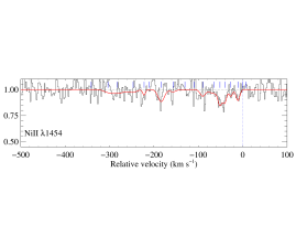
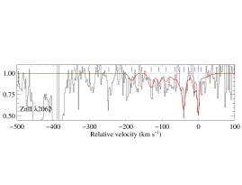
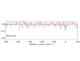
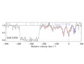
Figure 4: Multi-component Voigt-profile fit to singly ionised species (red), overlayed on top of the normalised UVES data. Regions marked in blue correspond to species other than labelled: e.g. the blue region in Si ii$\lambda$1808 is due to absorption by S i$\lambda$1807.

Table 2: Result of Voigt profile fitting to singly ionised metal lines.

$z_{\rm abs}$	$v$ (${\rm km\,s^{-1}}$)	$b$ (km s-1)	$\log N($SiII)	$\log N($NiII)	$\log N($ZnII)	$\log N($FeII)
2.521448	-341	6.64$\pm$ 0.91	13.31 $\pm$ 0.04			12.34 $\pm$ 0.08
2.521891	-303	13.26$\pm$ 1.61	14.21 $\pm$ 0.08	12.47 $\pm$ 0.54		13.59 $\pm$ 0.19
2.522135	-283	22.62$\pm$ 4.51	14.03 $\pm$ 0.15	13.08 $\pm$ 0.16		13.79 $\pm$ 0.13
2.522557	-247	12.26$\pm$ 0.68	14.31 $\pm$ 0.05	12.65 $\pm$ 0.20		13.72 $\pm$ 0.03
2.522848	-222	3.02$\pm$ 0.44	13.28 $\pm$ 0.07	12.54 $\pm$ 0.15		13.08 $\pm$ 0.04
2.522982	-211	4.49$\pm$ 0.98	13.14 $\pm$ 0.06			12.64 $\pm$ 0.06
2.523301	-184	9.52$\pm$ 0.28	14.80 $\pm$ 0.03	13.25 $\pm$ 0.05	12.07 $\pm$ 0.15	14.36 $\pm$ 0.03
2.523613	-157	9.16$\pm$ 1.08	13.96 $\pm$ 0.05	12.49 $\pm$ 0.24		13.50 $\pm$ 0.04
2.523930	-130	8.89$\pm$ 0.49	14.64 $\pm$ 0.04	11.81 $\pm$ 1.09	12.36 $\pm$ 0.07	14.00 $\pm$ 0.02
2.524179	-109	6.08$\pm$ 1.25	13.84 $\pm$ 0.10		12.06 $\pm$ 0.12	13.34 $\pm$ 0.06
2.524400	-90	7.58$\pm$ 0.92	14.53 $\pm$ 0.07	12.88 $\pm$ 0.10	12.04 $\pm$ 0.14	13.89 $\pm$ 0.05
2.524692	-65	13.37$\pm$ 6.16	14.41 $\pm$ 0.24	12.88 $\pm$ 0.25	12.14 $\pm$ 0.23	13.94 $\pm$ 0.21
2.524858	-51	5.25$\pm$ 1.32	14.72 $\pm$ 0.14	13.12 $\pm$ 0.14	12.01 $\pm$ 0.31	14.29 $\pm$ 0.13
2.524983	-41	4.93$\pm$ 0.77	14.93 $\pm$ 0.06	13.05 $\pm$ 0.10	12.65 $\pm$ 0.06	14.31 $\pm$ 0.09
2.525145	-27	4.31$\pm$ 0.76	14.33 $\pm$ 0.09	12.71 $\pm$ 0.12	11.70 $\pm$ 0.26	13.85 $\pm$ 0.05
2.525333	-11	5.06$\pm$ 0.43	14.99 $\pm$ 0.03	12.98 $\pm$ 0.07	12.25 $\pm$ 0.12	14.08 $\pm$ 0.05
2.525456	0	0.59$\pm$ 0.11	15.55 $\pm$ 0.41		14.03 $\pm$ 0.52	13.51 $\pm$ 0.43
2.525538	+7	26.22$\pm$ 2.94	14.06 $\pm$ 0.08		12.33 $\pm$ 0.25	13.66 $\pm$ 0.07
Total			15.93 $\pm$ 0.17	13.99 $\pm$ 0.04	14.09 $\pm$ 0.45	15.14 $\pm$ 0.03

We detect C ii lines in the UVES spectrum although these are saturated and do not provide any meaningful constraint on the column density of ionised carbon. In turn, the C ii${}^{*}\lambda$1335 fine-structure doublet lines are not apparently saturated as can be appreciated from Fig. 5. ${C\textsc{ii}}^{*}\lambda$1037 is unfortunately completely blended with intervening ${\rm Ly}\,\alpha$ forest absorption. Measuring the corresponding column densities remains therefore hazarduous due to the many components overlapping in the doublet and because the velocity decomposition differs from that of other metals. In addition, the strongest component is on the non-linear part of the curve of growth. We obtain $\log N({C\textsc{ii}}^{*})\sim 15$ in that component, with $b\sim 0.7$ ${\rm km\,s^{-1}}$. These values should be considered with great caution as the fit is sensitive to the initial guess, leading to uncertainties larger than an order of magnitude.

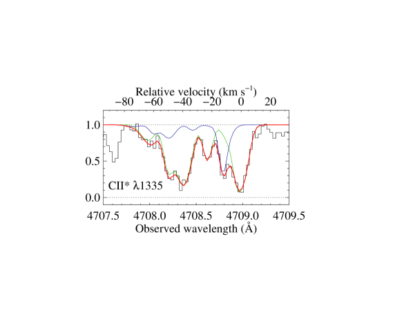
Figure 5: Fit to the C ii${}^{*}\lambda$1335 absorption profile (UVES data). The blue and green curves correspond to the contribution from each transition of the doublet. The top axis shows the relative velocity corresponding to the strongest transition (green, with $\lambda=$ 1335.7077 Å rest-frame).

3.3 Neutral carbon

The strong C i absorption lines that were used to select the system from the low-resolution SDSS spectrum are resolved in our UVES spectrum into different components and different fine-structure levels. We detect all three fine-structure levels of neutral carbon’s ground state triplet (2s²2p${}^{2}\,{}^{3}$P${}^{e}_{0,1,2}$) in five components, the strongest of which (by a factor of more than a hundred in column density) is associated with the narrow component seen in both the low-ionisation metal profile and in molecular absorption (H₂ and CO). We simultaneously fit all components from the fine-structure levels ($J$ = {0, 1, 2}, here denoted C i, C i^∗, C i^∗∗, respectively), tying Doppler parameters and redshifts for a given velocity component. We note that while this decreases the number of free parameters, it is based on the reasonable assumption that the fine-structure levels share the same physical origin. We use the lines at $\lambda_{\rm rest}\approx 1560$ and 1656 Å, located outside the ${\rm Ly}\,\alpha$ forest, to constrain the fit (see Fig. 6). Including other lines (e.g. C i$\lambda\lambda$1277,1328) does not improve the constraints due to the blends, lower S/N and lower spectral resolution. The results are provided in Table 3.

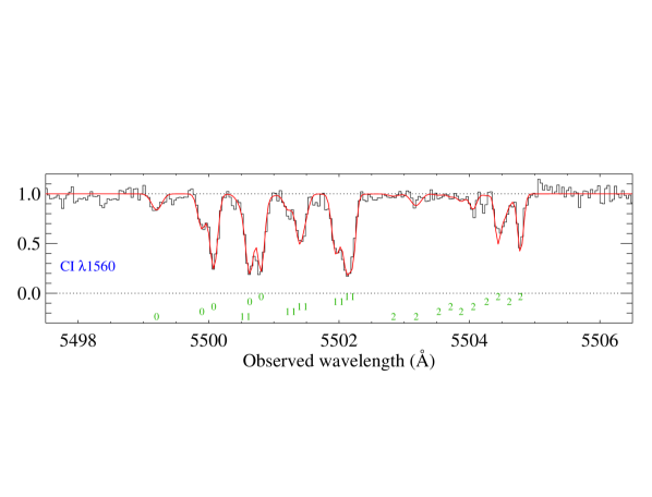
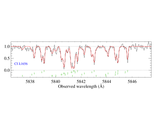
Figure 6: Fit to the neutral carbon lines (UVES data). The green numbers below each plot indicate the fine structure level $J$ for each of the five detected C i components.

Table 3: Column density of neutral carbon in differemt fine-structure levels

$z_{\rm abs}$	$b$ (km s-1)	$\log N($C i,J=0)	$\log N($C i,J=1)	$\log N($C i,J=2)
2.524432	4.96$\pm$ 0.71	12.76 $\pm$ 0.05	12.74 $\pm$ 0.11	12.69 $\pm$ 0.07
2.524876	3.41$\pm$ 0.67	13.05 $\pm$ 0.04	12.73 $\pm$ 0.07	12.38 $\pm$ 0.17
2.524993	2.57$\pm$ 0.32	13.61 $\pm$ 0.07	13.31 $\pm$ 0.03	12.67 $\pm$ 0.07
2.525347	2.84$\pm$ 0.26	13.65 $\pm$ 0.06	13.46 $\pm$ 0.02	12.46 $\pm$ 0.15
2.525458	0.81$\pm$ 0.04	16.10 $\pm$ 0.08	15.54 $\pm$ 0.14	14.67 $\pm$ 0.11

3.4 Molecular hydrogen

The spectrum of J0000$+$0048 is crowded with very strong Lyman (B${}^{1}\Sigma_{\rm u}^{+}(\nu^{\prime})$-X${}^{1}\Sigma_{g}^{+}(0)$) and Werner (C${}^{1}\Pi_{u}(\nu^{\prime})$-X${}^{1}\Sigma_{g}^{+}(0)$) lines from molecular hydrogen bluewards of 4000 Å (see Fig. 8). Since the X-Shooter spectrum has a much higher S/N and an extended wavelength coverage in the blue compared to the UVES spectrum, we use both spectra for the analysis of H₂, after normalising the spectra using a spline function. The UVES spectrum is particularly useful to identify regions blended with intervening ${\rm Ly}\,\alpha$ absorption from the forest, which are subsequently excluded during the fitting process.

Because the first ionisation potential of carbon, 11.26 eV, is very close to that of H₂ dissociation, carbon is usually considered as a good tracer of molecular hydrogen (e.g. Srianand et al., 2005). While there is no one-to-one correspondence, we can expect H₂ to be present in the five components in which C i is detected. Unfortunately, because H₂ lines are strongly saturated, it is impossible to distinguish several close components in their profile. We therefore measure only the total H₂ column density by modelling the absorption profile using a single velocity component. This should be dominated by the reddest narrow component, for which the C i column density is about two orders of magnitude higher than in the rest of the components. We tie together the redshifts for the different H₂ rotational levels, under the assumption that they arise from the same physical cloud. Absorption lines for the low rotational levels ($J\leq 2$) are damped, meaning that the column density is well constrained while the profile does not directly depend on (and therefore does not constrain) the Doppler parameter.

Figure 7 shows the excitation diagram of H₂, which presents the population in each rotational level against the energy of that level:

$${{N({\rm H}_{2},J^{\prime})}\over{g({\rm H}_{2},J^{\prime})}}={{N({\rm H}_{2},J)}\over{g({\rm H}_{2},J)}}e^{-E_{JJ^{\prime}}/kT_{JJ^{\prime}}},$$ (1)

where $E_{JJ^{\prime}}$ is the energy difference between levels $J$ and $J^{\prime}$, $g({\rm H}_{2},J)$, $g({\rm H}_{2},J^{\prime})$ are the respective spin statistical weights and $T_{JJ^{\prime}}$ is the excitation temperature. $T_{01}$ is generally considered as a very good indicator of the kinetic temperature of the gas at such high column density, where selective self-shielding is no longer at play and the low rotational levels are easily thermalised thanks to short collisional time-scales (Roy et al., 2006; Le Petit et al., 2006). In turn, the high rotational levels are characterised by a higher excitation temperature. This is expected and seen in interstellar clouds because of the very slow infrared relaxation after UV or formation pumping into high-$J$ levels. Moreover collisional de-excitation becomes difficult at the high-$J$ levels, where the level spacings become so large (several hundred cm^-1) that these amounts of energy cannot be transferred in collisions, in particular at the density and temperatures seen in the ISM. This leads to the observed non-Boltzmann distribution. We also note that the observed excitation diagram corresponds to integrated values and that possible additional warmer components with lower $N($H₂) will mostly contribute to the high-$J$ levels.

We measure $T_{01}=51\pm 2$ K, which is lower than the value typically seen in H₂-bearing DLAs (Srianand et al., 2005, $T\sim 150$ K), and closer to what is seen in our Galaxy, with an average of about 77 K (Rachford et al., 2002). The kinetic temperature $T_{\rm kin}\approx T_{01}$ corresponds to a Doppler parameter for H₂ of $b_{\rm th}\approx 0.65$ ${\rm km\,s^{-1}}$ if we assume thermal broadening only. However, because turbulent broadening is also likely present, as indicated by similar Doppler parameters for much heavier species, this value should be considered as a lower limit to the line broadening. We can get a more realistic estimate of the Doppler parameter by quadratically adding this pure thermal value to the turbulent $b$-value seen for heavier species (for which $b_{\rm th}$ is negligible, see Fig. 16) and obtain $b=\sqrt{b_{\rm th}^{2}+b_{\rm turb}^{2}}\approx$1.0 ${\rm km\,s^{-1}}$.

However, it has been observed in several H₂-bearing systems that the Doppler parameter can also be an increasing function of the rotational level (e.g. Lacour et al., 2005; Noterdaeme et al., 2007; Albornoz Vásquez et al., 2014), possibly due to more turbulent an warmer external layers where UV pumping of H₂ is enhanced (Balashev et al., 2009). We therefore also perform a fit using a high $b$-value of 5 ${\rm km\,s^{-1}}$. The resulting parameters are provided in Table 4. We obtain a total column density of $\log N$(H${}_{2})=20.43\pm 0.02$ which implies an overall molecular fraction, $f=2N($H${}_{2})/(2N($H${}_{2})+N({H\textsc{i}}))=0.46\pm 0.07$, i.e. the highest value measured to date in a quasar-DLA. This also corresponds to a strict lower limit to the molecular fraction in the cold component.

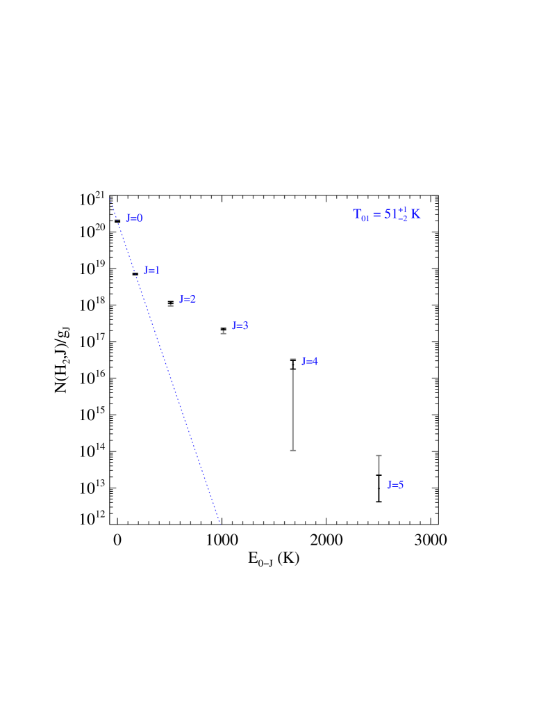
Figure 7: H₂ excitation diagram. The black points and error bars correspond to the fit with $b=1.0$ ${\rm km\,s^{-1}}$. Grey error bars correspond to extrema with $b=0.65$ and $5$ km s^-1.

Table 4: Column density in different rotational levels of H₂ for the three values of the Doppler parameter.

Rot. level	$\log N($H${}_{2},J)$
($J$)	$b=1.0$	$b=0.65$	$b=5$
	(km s-1)	(km s-1)	(km s-1)
0	20.29 $\pm$ 0.02	20.29 $\pm$ 0.02	20.31 $\pm$ 0.02
1	19.81 $\pm$ 0.02	19.80 $\pm$ 0.02	19.79 $\pm$ 0.02
2	18.77 $\pm$ 0.03	18.77 $\pm$ 0.03	18.70 $\pm$ 0.03
3	18.67 $\pm$ 0.02	18.67 $\pm$ 0.02	18.57 $\pm$ 0.03
4	17.32 $\pm$ 0.12	17.37 $\pm$ 0.11	15.08 $\pm$ 0.10
5	14.50 $\pm$ 0.36	14.79 $\pm$ 0.62	14.42 $\pm$ 0.16
Total	20.43$\pm$0.02	20.43$\pm$0.02	20.44$\pm$0.02

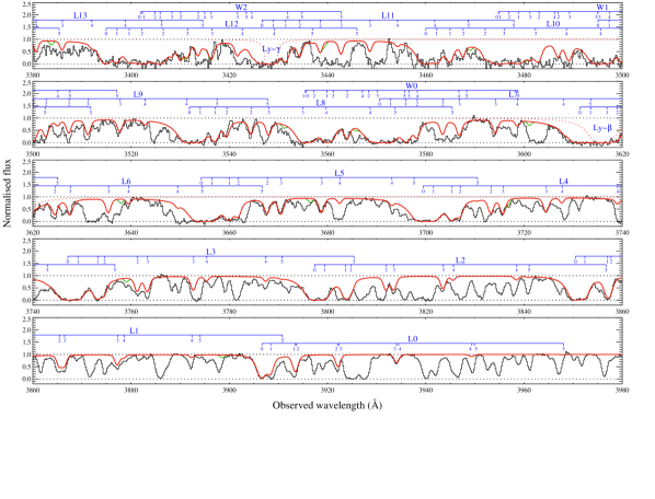
Figure 8: Portion of X-Shooter UVB spectrum (black) around the H₂ lines, with the best-fit synthetic spectrum for H₂ absorption (with $b=1$ ${\rm km\,s^{-1}}$) in red. Horizontal blue segments connect rotational levels (short tick marks) from a given Lyman (L) or Werner (W) band, as labelled above. H i Ly-$\beta$ and Ly-$\gamma$ from the DLA are indicated as red dashed profiles. The green profile corresponds to HD lines.

3.5 Deuterated molecular hydrogen

Several lines of deuterated molecular hydrogen are also detected in both the UVES and X-Shooter spectra. However, HD lines are often blended with ${\rm Ly}\,\alpha$ forest or H₂ absorption and are saturated in the low S/N UVES spectrum but weak in the medium resolution X-shooter spectrum. We therefore use here on a different fitting procedure based on Markov Chain Monte Carlo method. We considered L0R0, L4R0, L5R0, L6R0, L8R0 and W0R0, locally re-normalised, as well as L11R0 and L14R0 (covered only by X-Shooter). We use two components with fixed redshifts ($z=2.525458$ and $z=2.525348$) corresponding to the strongest components seen in C i and use C i Doppler parameters as priors. The synthetic HD profiles in the UVES spectrum are shown on Fig. 9 and the corresponding X-Shooter profile also included in Fig. 8. We only consider the total HD column density as being reasonably trustable, with $\log N_{\rm HD}=16.64^{+0.16}_{-0.18}$. This corresponds to ${\rm HD/2H_{2}}=(8.1^{+3.7}_{-2.8})\times 10^{-5}$, which is significantly higher than the typical ratios observed in our Galaxy (Snow et al., 2008) and than the primordial value estimated from D i/H i in low metallicity high-$z$ DLAs ((D/H)${}_{\rm p}=(2.53\pm 0.04)\times 10^{-5}$; Cooke et al., 2014). While a high abundance of deuterium can possibly be explained by strong supply of primordial gas (as suggested by Ivanchik et al., 2010), the molecular ratio is here more likely explained by chemical fractionation and charge exchange processes (Liszt, 2015). Without entering into details of the HD chemistry, we note that the reaction ${\rm D^{+}+H_{2}}\to{\rm HD+H^{+}}$ is fast and can lead to an increasing of HD compared to H₂. If we call $f_{\rm HD}={\rm HD/(HD+{D\textsc{i}})}$ the fraction of deuterium in molecular form, then we have

$${{\rm HD}\over 2{\rm H_{2}}}=\left({D\over H}\right){{f_{\rm HD}}\over{f_{\rm H2}}}$$ (2)

Assuming an intrinsic primordial value, the high ${\rm HD}/{\rm H_{2}}$ ratio can be explained for $f_{\rm HD}/f_{\rm H2}\simeq 3.2$, which would naturally require that the cloud cannot be fully molecular. This is indeed what we conclude from modelling the physical conditions in the cloud (Sect. 6). We however caution that a high-resolution spectrum with high S/N ratio is necessary to better take into account blends with the Ly-$\alpha$ forest and confirm our measurement.

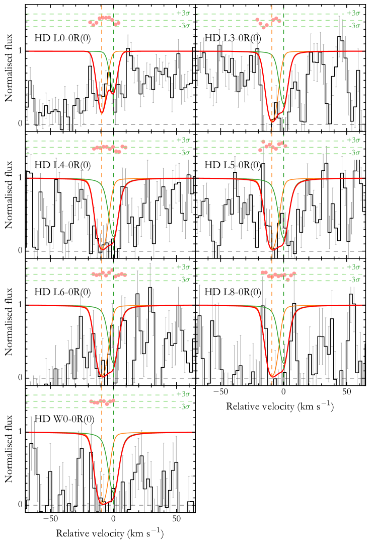
Figure 9: HD synthetic profile overlaid on the UVES spectrum.

3.6 Neutral chlorine

Chlorine is known to be tightly linked with H₂ thanks to rapid chemical reactions (e.g. Jura, 1974a). In our Galaxy, observations of clouds with $\log N($H${}_{2})>19$ using the Copernicus satellite have revealed a clear correlation between the column density of both species (Moomey et al., 2012). Recently, Balashev et al. (2015) used a sample of known H₂-bearing DLAs to show that this relation stands at high redshifts and down to ten times lower column densities. Here, only one absorption line of neutral chlorine, Cl i$\lambda$1347 is covered and not blended in our spectrum. Three components, that match those seen in the neutral carbon profile are detected and used to constrain the column densities, while those associated to the weakest C i components are below our detection limit. This again indicates that H₂ should actually be present in more than one component, although too close to be distinguished within the damped profile of the strong, cold component. Unfortunately, the column density of neutral chlorine in that component is poorly constrained because this line is in the intermediate regime with a strong dependence on the Doppler parameter. Therefore, the Voigt profile fit keeping all parameters free leads to a very high uncertainty in the column density. However, we can make the reasonable assumption that the Doppler parameter should be close to that of other species for this component. Since chlorine is expected to arise from the H₂-bearing gas but with a much higher atomic mass, its thermal broadening should be negligible and its Doppler parameter close to that of other “heavy” species. Assuming $b=0.7$ ${\rm km\,s^{-1}}$(see Fig. 16) we obtain a very satisfactory fit with $\log N({Cl\textsc{i}})=14.6\pm 0.3$ in the narrow component. We also fitted Cl i assuming a more relaxed constraint on $b$, that we take in the range 0.6-0.8 ${\rm km\,s^{-1}}$, giving $\log N({Cl\textsc{i}})=14.43-14.89$ with a similar 0.3 dex fitting uncertainty. This sets the overall uncertainty to about 0.4 dex. The results are shown in Fig. 10 and Table 5, where we also provide the fitting results leaving the Doppler parameter totally free, for completeness.

Table 5: Neutral chlorine fitting parameters

$z_{\rm abs}$	$b$	$\log N({Cl\textsc{i}})$	$b$	$\log N({Cl\textsc{i}})$
	(${\rm km\,s^{-1}}$)		(${\rm km\,s^{-1}}$)
2.52500	6.5$\pm$1.3	13.00$\pm$0.06	6.6$\pm$1.2	13.00$\pm$0.06
2.52536	4.8$\pm$1.5	13.03$\pm$0.10	4.9$\pm$1.1	13.04$\pm$0.06
2.52546	0.8$\pm$0.6	14.55$\pm$1.92	0.7	14.63$\pm$0.29
Total		14.58$\pm$1.81		14.65$\pm$0.27

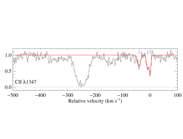
Figure 10: Fit to the absorption profile of neutral chlorine.

3.7 Neutral sulphur

Because the first ionisation potential of sulphur is 10.36 eV, neutral sulphur is only expected to be found in very shielded regions. To our knowledge, only a handful detections of S i have been reported so far in DLAs, all associated to a molecular absorber featuring CO (Srianand et al., 2008) and/or strong H₂/HD (Milutinovic et al., 2010; Balashev et al., 2011). Here, we detect S i absorption lines with $\log N({S\textsc{i}})=14.85\pm 0.18$ in our UVES spectrum from five transitions in a single narrow ($b=0.50\pm 0.07$ ${\rm km\,s^{-1}}$) component, see Fig. 11. This suggests that S i can be used as a tracer for CO (Noterdaeme et al., 2010), just like the presence of C i implies that of H₂. However, because S i lines have similar strengths and are located in the same spectral region as CO lines, this is of little practical use to identify CO systems. Still, S i can be helpful in determining the velocity structure of multi-component CO absorption systems (e.g. Srianand et al., 2008; Noterdaeme et al., 2009a).

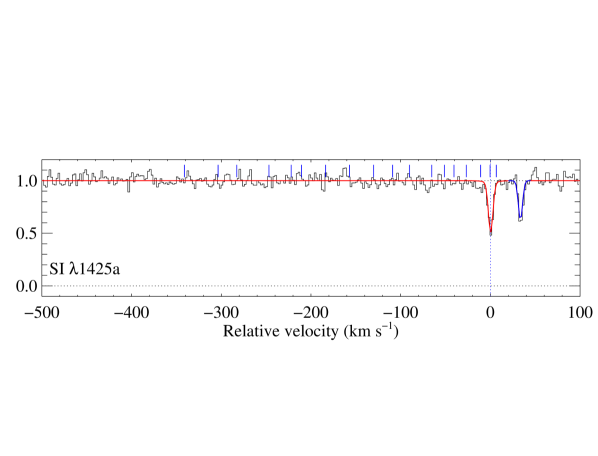
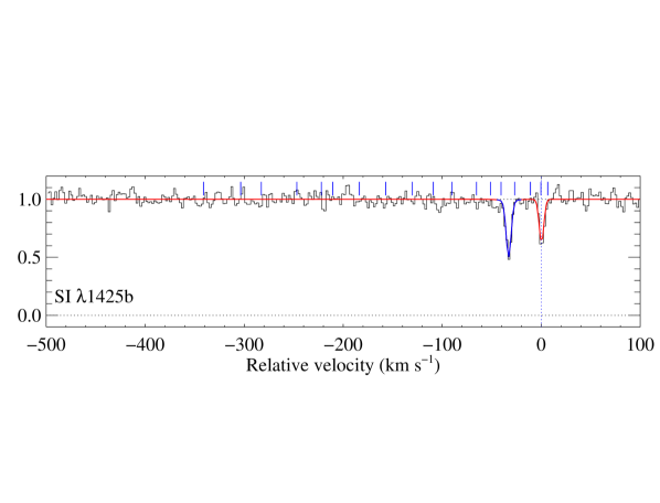
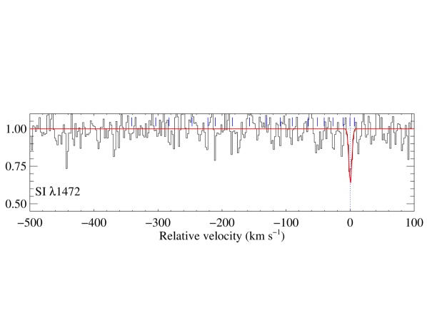
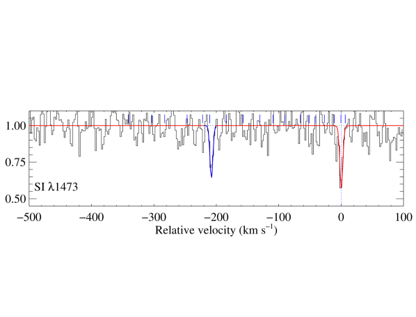
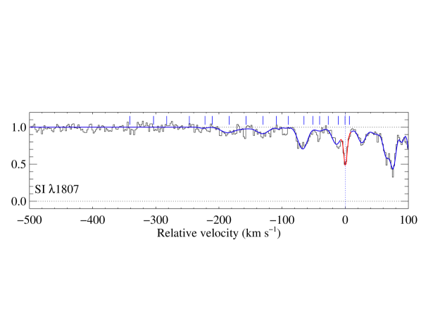
Figure 11: Neutral sulphur absorption lines (UVES data). As for Fig. 4, the continuous red line correspond to the best fit model, with regions corresponding to other absorption lines marked in blue (for example, most of the profile seen in the S i$\lambda$1807 actually corresponds to Si ii$\lambda$1808, except around $v=0$ ${\rm km\,s^{-1}}$). The short tick marks show the position of the singly ionised metal lines. Note that S i is detected only in the component that has CO.

3.8 Neutral magnesium and neutral sodium

Neutral magnesium (Mg i) is detected in five transitions in our UVES spectrum (see Fig. 12). We clearly detect two components and possibly two additional weak components. The main component, again corresponding to the molecular one at $v=0$ ${\rm km\,s^{-1}}$, contains more than 80% of the total column density with $\log N({Mg\textsc{i}})_{\rm c}=14.1\pm 0.1$ . Interestingly, the hidden saturation of this component with very small Doppler parameter ($b=0.86\pm 0.1$ ${\rm km\,s^{-1}}$) is directly evidenced by its relative strengths to the second strongest component: both these components have similar observed optical depth for ${Mg\textsc{i}}\lambda 2026$, but the former is also seen in transitions with much smaller oscillator strengths.

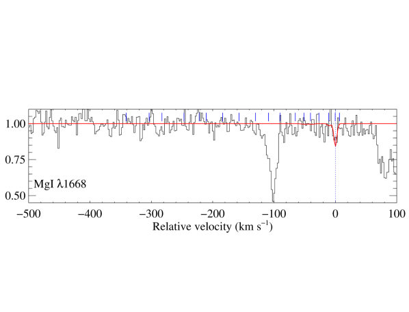
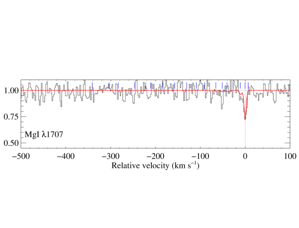
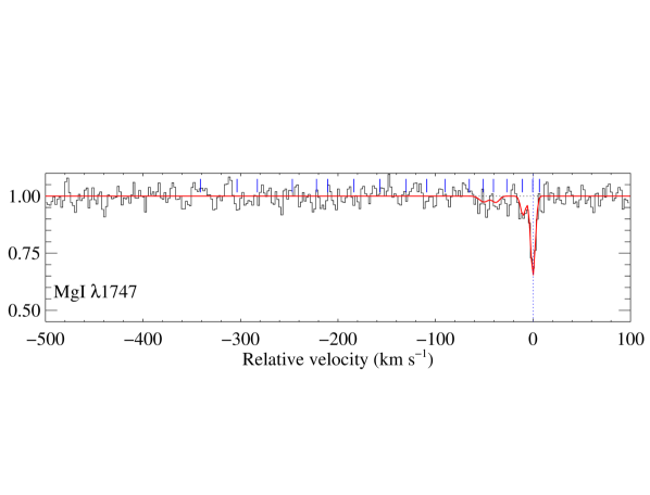
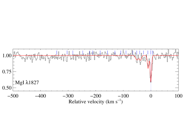
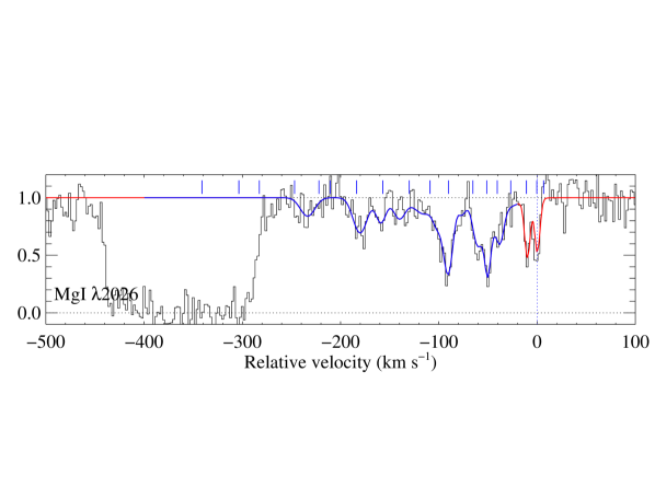
Figure 12: Fit to the neutral magnesium absorption lines (UVES data). The blue region in the bottom panel corresponds to Zn ii$\lambda$2026.

We also detect the Na i$\lambda\lambda$5891,5897 doublet in the NIR X-Shooter spectrum. The non-gaussian profile indicates that several components are present, although blended at the achieved spectral resolution (around $R\sim$8500). We therefore use the velocity decomposition of Mg i obtained at high spectral resolution, i.e., the redshifts and Doppler parameters of Na i are fixed to the value previously determined for Mg i and only the column density is allowed to vary. This assumption leads to a good fit of the observed Na i absorption features (Fig. 13), with a column density in the main component of $\log({Na\textsc{i}})_{c}=15.0\pm 0.3$, with a large fitting uncertainty due to the line being much narrower than the resolution element. We also note that the value is very dependent on the exact normalisation and that the first ionisation potential of sodium (5.14 eV) is even lower than that of magnesium (7.65 eV), meaning that Na i may arise from deeper regions in the cloud. This means that Na i column densities should be considered with great caution until a high resolution infra-red spectrum is obtained. Using the empirical correlation observed in the Milky Way between Na i equivalent width and $E(B-V)$ from Poznanski et al. (2012), we expect $A_{\rm V}\sim 0.3$ for their implicitely assumed $R_{V}=3.1$. We will see in Sect. 5 that this is not far from the observed value.

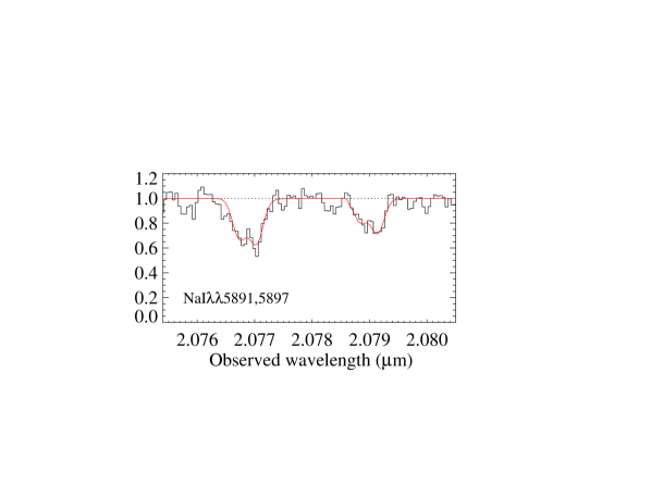
Figure 13: Portion of the X-Shooter NIR spectrum around the Na i doublet. Na i$\lambda$5891 and Na i$\lambda$5897 are redshifted at 2.077 and 2.079$\mu$m, respectively. The red curve corresponds to the Voigt-profile fit using fixed velocity decomposition from Mg i.

3.9 Carbon monoxide

We detect CO absorption lines from ten bands, belonging to two systems: the A${}^{1}\Pi(\nu^{\prime})$-X${}^{1}\Sigma^{+}(0)$ for $\nu^{\prime}=0$ to 8 and the d${}^{3}\Delta(5)$-X${}^{1}\Sigma^{+}(0)$ inter-band system, see Fig. 14. We also tentatively detect the e${}^{3}\Sigma^{-}$-X${}^{1}\Sigma^{+}$ system, although the lines remain too weak to be significant (Fig. 15). Rotational levels are unambiguously detected from J=0 to J=3. The J=4 lines are at the noise level for most bands, but included in the fit. We used updated molecular data summarised in Daprà et al. (2016). Accurate wavelengths were obtained through calibration by laser and VUV synchrotron studies (Salumbides et al., 2012; Niu et al., 2013, 2015), while oscillator strengths and damping constants were carefully re-evaluated taking into account an updated pertubation analysis. We do not consider the $\nu^{\prime}=5$ AX system, which is completely blended with the extended Si iv$\lambda$1393 absorption. Similarly, a large region of the (2-0) absorption band is contaminated by unrelated absorption and ignored during the fitting. Finally, the (6-0) band is also partially blended with smooth absorption from the ${\rm Ly}\,\alpha$ forest, but the latter is well modelled using a single component. We therefore included this band and left the intervening ${\rm Ly}\,\alpha$ parameters free during the fitting process. The other CO bands are apparently free from blending. We tied together the Doppler parameter and redshift for the different rotational levels. We are therefore left with seven free parameters for CO: $b$, $z$ and the column densities for the 5 detected rotational levels. We obtain a satisfactory fit with a global $\chi^{2}_{\nu}=1.1$, shown as the red profile in Fig. 14, with $z=2.525467$, $b=0.7$ ${\rm km\,s^{-1}}$ and obtain a total CO column density of almost 10¹⁵ ${\rm cm}^{-2}$, which is the highest measured among high-$z$ quasar absorption systems to date. We further test the robustness of our measurement in the appendix.

From the non-detection of ¹³CO lines, we also constrain the isotopic ratio ¹²CO$/^{13}$CO to be higher than 40, assuming the same Doppler parameter, redshift and excitation temperature for both molecules. This is comparable with values in the Solar neighbourhood (¹²CO$/^{13}$CO$\sim 70$; Sheffer et al., 2007), meaning that a measurement of the CO isotopic ratio at high-$z$ should be possible in the near future. This is particularly interesting since the isotopic ratio seems to be anticorrelated with $N$(CO) in the Galaxy, indicating ¹³CO enhancement through chemical fractionation in the denser and colder regions (e.g. Sonnentrucker et al., 2007).

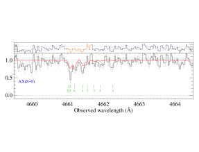
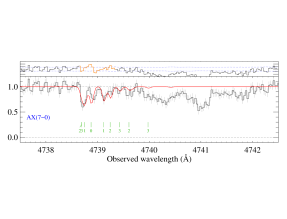
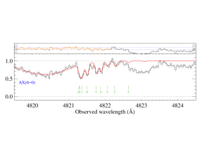
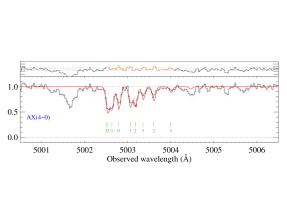
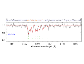
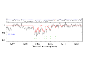
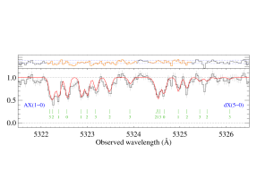
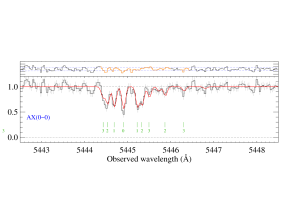
Figure 14: Voigt-profile fit to the CO absorption bands labelled in blue in each panel (UVES data). Rotational levels from $J=0$ to $J=3$ are indicated as green tick marks. The panel above each region shows the residuals where the blue line indicates the $\pm$1 $\sigma$ interval, and the orange regions mark those used to constrain the fit.

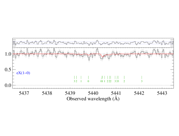
Figure 15: Tentative detection of $(1-0)$ band of the e${}^{3}\Sigma^{-}$-X${}^{1}\Sigma^{+}$ CO system (UVES data). The red profile correspond to the calculated synthetic spectrum, using the parameters obtained from fitting the AX and dX bands and molecular data from Eidelsberg & Rostas (2003).

Table 6: CO best-fit parameters

Rot. level ($J$)	$\log N($CO,$J)$	$b$ (km s-1)
0	14.43$\pm$0.12	0.71$\pm$0.03
1	14.52$\pm$0.08	”
2	14.33$\pm$0.06	”
3	13.73$\pm$0.05	”
4	13.14$\pm$0.13	”
Total	14.95$\pm$0.05	”

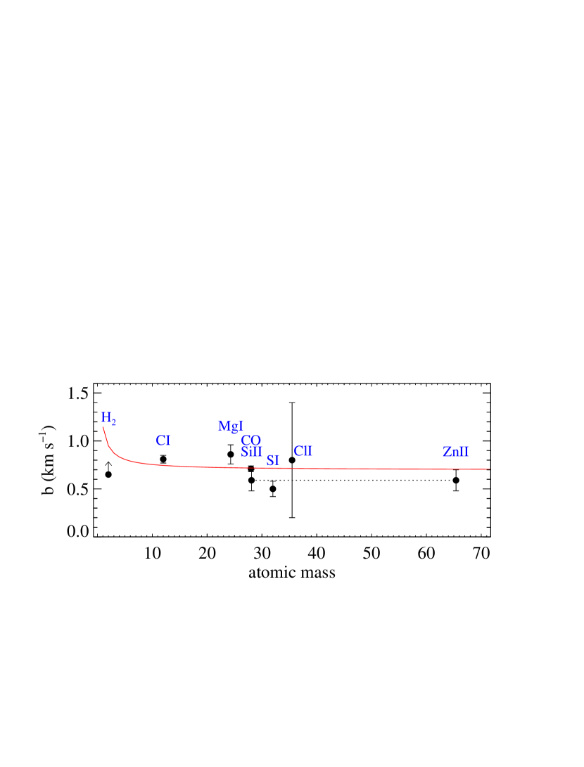
Figure 16: Doppler parameters and associated 1 $\sigma$ uncertainties for different species in the cold component. The red curve represents the expected $b$-value for $T=50$ K and $b_{\rm turb}=0.7$ ${\rm km\,s^{-1}}$. Note that the values for Si ii and Zn ii were tied together during the fit. The lower-limit to $b$(H₂) corresponds to thermal broadening only.

4 Metallicity and dust depletion

4.1 Metallicity in the atomic and molecular gas

In this section, we briefly discuss the metallicity in the different phases. We denote the abundance of a species M relative to hydrogen as

$$[{\rm M/H}]\equiv\log(N({\rm M})/N({\rm H}))-\log(N({\rm M})/N({\rm H}))_{\odot}.$$ (3)

where Solar abundances are taken from the photosperic values of Asplund et al. (2009). H corresponds to the total hydrogen, i.e. including both neutral (H i) and molecular (H₂) forms. We measure $\log(N({H\textsc{i}})+2N($H${}_{2}))=21.07$. Using the undepleted zinc, we derive an overall super Solar metallicity, [Zn/H] = +0.46$\pm$0.45, where the large uncertainty is due to that on the narrow component which contains most of the metals. Using phosphorus, we derive [P/H]$>$-0.04. This is a lower limit because only the strongest components are detectable and because of some phosphorus depletion in the ISM (by about 0.2 to 0.5 dex, see e.g. Lebouteiller et al., 2005). While this is here again consistent with super-Solar metallicity, it also indicates that the upper range from Zn ii is less likely.

It is remarkable that if we assume a molecular fraction of one in the cold component and zero elsewhere, then we get a lower limit to the metallicity of the “warm” gas to be [Zn/H]${}_{\rm w}\geq-0.2\pm 0.1$, i.e., still consistent with Solar. We also note that the bluest components ($v<-200$ ${\rm km\,s^{-1}}$) of zinc could not be constrained because of blending with unrelated lines, but these are expected to account for a marginal fraction of the total metal column anyway. Using Si ii we obtain [Si/H]${}_{\rm w}>-0.6$. This should be considered as a conservative lower limit since silicon depletion is expected to occur (see indeed Sect. 4.2).

While we cannot measure the H i column density in individual components, we can expect that the metallicity in the cold component is at least as high as in the rest of the profile and obtain a more realistic lower limit. We assume

$${\rm[Zn/H]_{c}\geq[Zn/H]_{\rm overall}},$$ (4)

where the index $c$ stands for “cold”, i.e. associated to the molecule-bearing gas. The molecular fraction in the cold component, $f_{\rm c}=2N($H${}_{2})/(2N($H${}_{2})+N({H\textsc{i}})_{\rm c})$ can then be expressed as

$$f_{\rm c}\ga f{{N({Zn\textsc{ii}})_{\rm overall}}\over{N({Zn\textsc{ii}})_{\rm c}}}\approx 0.54.$$ (5)

Conversely, if we assume that the cold component is fully molecular (i.e. $f_{c}=1$), we get an upper-limit to the metallicity in that component, [Zn/H]${}_{c}<0.7\pm 0.5$, while the lower-limit to the metallicity in the warm gas is [Zn/H]${}_{\rm w}>-0.2$ (see Sect. 3.2).

Because chlorine is associated to the H₂-bearing gas, its abundance can also be used to constrain the metallicity of the latter using the relation from Balashev et al. (2015)

$${\rm[Cl/H]}={\rm[Cl/H_{2}]}+\log{f},$$ (6)

where

$${\rm[Cl/H_{2}]}=\log\left(\frac{N({\mbox{Cl})}}{2N({\rm H}_{2})}\right)-\log\left(\frac{{\rm Cl}}{{\rm H}}\right)_{\odot}.$$ (7)

We measure [Cl/H₂]$\sim$0.4$\pm$0.3 using the fit with fixed Doppler parameter for the main component. The lower limit to the molecular fraction $f>0.46$ (see Sect. 3.4) then implies [Cl/H] $>$ 0.05$\pm$0.3 in the cold component. This is a strict limit on the metallicity since several studies have argued for some depletion of chlorine, by about a factor of two (see e.g. Moomey et al., 2012, and references therein). The abundance of chlorine is therefore consistent with the super-solar metallicity derived from zinc and phosphorus, assuming instrinsic solar ratio. We also note that assuming uniform metallicity across the different components implies that about 95% of H₂ resides in the main component.

4.2 Dust abundance from depletion of refractory elements

Ledoux et al. (2003) have revealed the existence of a relation between the presence of molecular hydrogen and both the overall metallicity (see also Petitjean et al., 2006) and the observed depletion factors in DLAs, i.e., the probability to detect H₂ is higher when the relative abundances of metals (or dust) are high. Noterdaeme et al. (2008) further showed that the column density of H₂ is strongly related to that of dust, quantified by the column density of iron missing from the gas phase ($N({\rm Fe_{dust}})$, Vladilo et al., 2006). However, the metallicity and depletion factors are only indicative of the average values over the whole absorption path probed by the DLA while the $N({\rm Fe_{dust}})$ corresponds to an integrated value. Indeed, metals probe gas over a wide range of physical conditions, making it generally difficult to associate a given metal component to a molecular one. Still, it has been possible to show that abundance ratios along the velocity profiles tend to show an enhanced depletion factor at the velocity where H₂ is detected (Rodríguez et al., 2006).

The system towards J0000$+$0048 presents an excellent opportunity to study this further, since the metal profile presents a well defined narrow component corresponding to the molecular gas. Fig. 17 presents the observed depletion factors (Si, Ni and Fe relative to Zn) component by component. The three patterns follow well each other, indicating that the abundances ratios are mainly dictated by depletion onto dust grains, rather than differential nucleosynthesis. As expected, the cold narrow component presents a high level of dust depletion, indicating that this component has a high relative amount of dust. However, a dusty component does not necessarily have a high integrated column density of dust, which will be more naturally related to the column density (and hence detectability) of molecular species. We therefore compute the column density of iron locked into dust grains component by component. The cold, molecule-rich component becomes clearly visible and likely responsible for most of the extinction of the background quasar (see next section). We also notice a secondary peak at $v\approx-40$ ${\rm km\,s^{-1}}$. Interestingly, this corresponds to the location of a neutral chlorine component, which also likely harbours H₂ molecules, though with a lower column density. This suggests that neutral chlorine could be directly used as a “high-resolution” tracer of dust within a DLA.

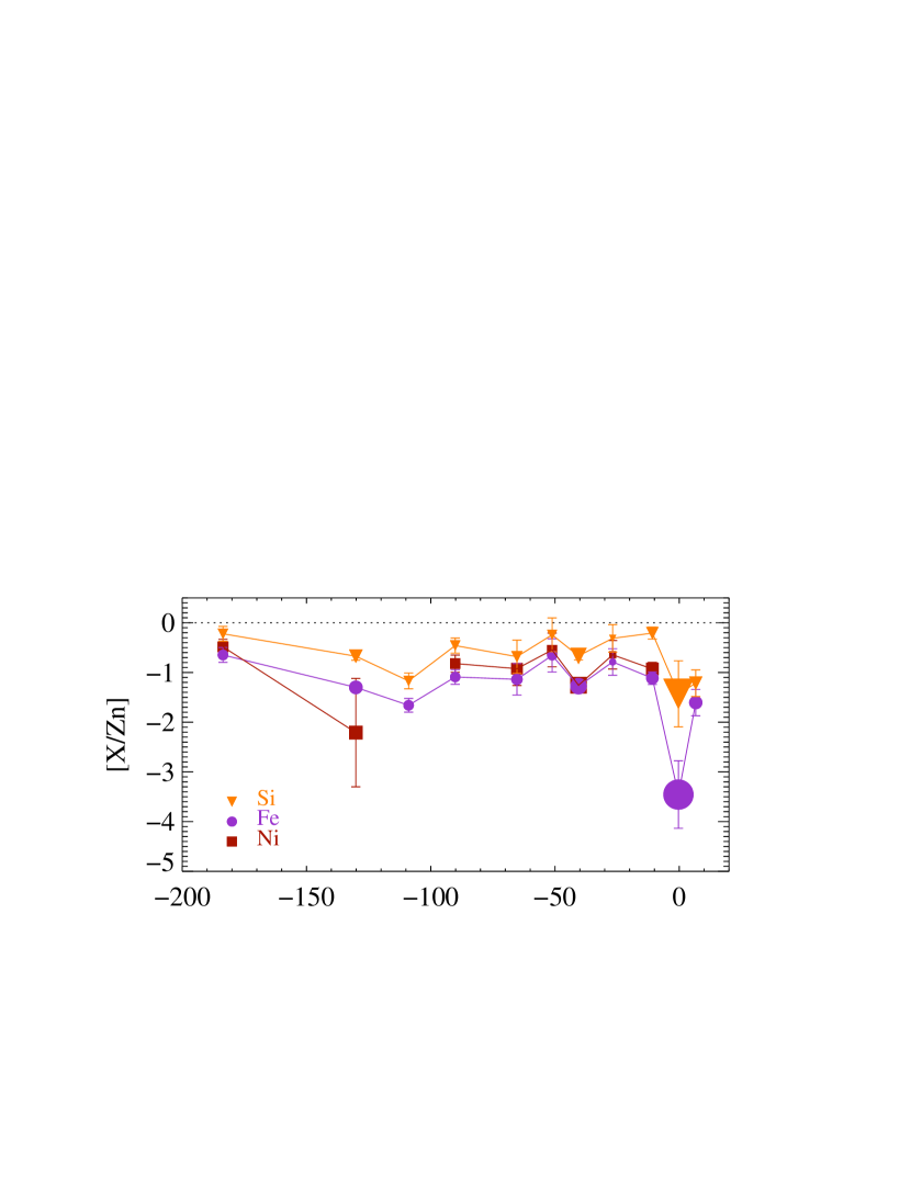
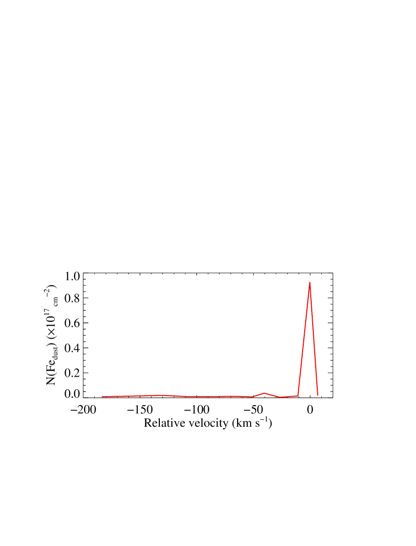
Figure 17: Top: Depletion of silicon, iron and nickel relative to zinc in individual components (left axis). Note that several [Ni/Zn] are not available due to the column density of nickel being less than the detection limit. The size of each point is representative of the corresponding Zn ii column density. Bottom: Column density of iron locked into dust.

5 Extinction of the background quasar light

The spectrum of the quasar J0000$+$0048 shows clear signs of being reddened, with a clear 2175 Å absorption bump at the redshift of the DLA. This, together with the detection of neutral and molecular species strongly suggests that the dust reddening is caused by the absorber. In the following analysis, we use the quasar template of Selsing et al. (2016).

Instead of assuming a fixed extinction curve parametrisation (e.g., Small Magellanic Cloud type as typically assumed in the litterature), we are able to constrain the extinction curve towards this quasar in high detail thanks to the long wavelength coverage of X-Shooter. For this purpose, we define continuum regions in the observed spectrum which are not strongly influenced by absorption (both telluric and from the DLA) or broad emission lines. In the near-infrared, we perform a 5-$\sigma$ clipping in order to discard outliers introduced by the removal of skylines in the data reduction. We include photometry in the $K$-band from the UKIRT Infrared Deep Sky Survey (UKIDSS) and in band 1 from the Wide-Field Infrared Survey Explorer (WISE). We are not able to include the redder bands from WISE, since the quasar template at this redshift only covers part of band 2 at 4.6 $\mu$m. However, we observe an offset between the UKIDSS photometry and the SDSS and WISE photometry. This is most plausibly due to variability of the quasar between the different epochs of observation. In order to correct for this offset, we scale the spectrum to the $z$-band of the SDSS photometry and subsequently scale the four UKIDSS bands to match the synthetic photometry calculated from the scaled spectrum.

The template of Selsing et al. is then smoothed with a Gaussian kernel ($\sigma$ = 7 pixels) to prevent the noise in the template to falsely fit noise peaks in the real data. In order to take into account the uncertainty in the template, we convolve the errors on the spectrum with the uncertainty estimate from the template.

We then fit the template to the data using 9 free parameters: 7 parameters to describe the extinction curve shape, a freely varying amount of dust, $A_{V}$, and an arbitrary scale since we do not know the intrinsic brightness prior to reddening.

5.1 Parametrisation of the extinction law

We use a slightly modified version of the formalism from Fitzpatrick & Massa (2007, hereafter, FM2007):

$$k(\lambda-V)=E(\lambda-V)/E(B-V)=c_{1}+c_{2}x+c_{3}D\leavevmode\nobreak\ ,$$ (8)

where

$$D=\frac{x^{2}}{(x^{2}-x_{0}^{2})^{2}+x^{2}\gamma^{2}}$$ (9)

and $x=\lambda^{-1}$ refers to inverse wavelength in units of $\mu$m^-1 at the absorber rest-frame. This corresponds to a linear component for the whole UV range (defined by $c_{1}$ and $c_{2}$) plus a 2175Å̃ bump, parametrised by $c_{3}$, $x_{0}$ and $\gamma$. FM2007 also consider a far-UV curvature component parametrised by $c_{4}$ at wavelengths shorter than $c_{5}$ (their Eq. 2). We do not consider this component here (i.e. we set $c_{4}=0$) because we do not have enough data in the FUV and the quasar template is more uncertain at very short wavelengths. In addition, preliminary fits to the data indicate that $c_{4}$ is little constrained and fully consistent with $0$. We therefore exclude it in the following analysis to simplify the fit without loss of generality.

In the infrared (IR), we use the power-law prescription of FM2007 assuming the correlation between $k_{\rm IR}$ and $R_{\rm V}$, thus yielding an extinction curve of the form (eq. 7 of FM2007):

$$k(\lambda-V)=(-0.83+0.63\times R_{V})\times x^{1.84}-R_{V}$$ (10)

Since this part of the extinction curve is beyond the spectral coverage we choose to reduce the two original IR parameters, by including the correlation between $k_{\rm IR}$ and $R_{V}$. We use a spline interpolation as in FM2007, in the optical range using one anchor point in the optical to ensure a correct normalisation in the $V$-band. In order to obtain a smooth and continuous transition between the various parts, we include two anchor points in the UV and two in the IR. We use the UV points $U_{1}$ and $U_{2}$ as defined in FM2007 at 2600 and 2700 Å, respectively. In the IR, we anchor the spline at 0.75 and 1.0 ${\rm\mu m}^{-1}$ (similar to the $I_{4}$ and $I_{5}$ points of FM2007).

Finally, we convert the extinction curve from the original formulation in terms of $E(\lambda-V)$ to use $A_{\lambda}$:

$$A_{\lambda}/A_{V}=\frac{1}{R_{V}}E(\lambda-V)/E(B-V)+1.$$ (11)

5.2 Fitting the extinction

We fit the parameters using a Markov Chain Monte Carlo method as implemented in the python package emcee (Foreman-Mackey et al., 2013). This way we can include priors and parameter boundaries in a straightforward way. The shape parameters for the 2175 Å bump, $x_{0}$ and $\gamma$, are given quite strong priors, since these parameters are observed to be very well behaved in many different environments (Fitzpatrick & Massa, 1990; Gordon et al., 2003). As priors on the two parameters, we use the average values from Gordon et al. (2003), $x_{0}=4.57\pm 0.01$ and $\gamma=0.94\pm 0.02$.

In order to give the photometry a more appropriate weight compared to the densely sampled spectral data, we calculate an effective number of pixels per filter. We calculate this quantity by integrating the filter transmission curves scaled to a maximum of $1$ and interpolated onto a grid with the same sampling as the spectral data. This way, pixels with high transmission are weighted more than ‘pixels’ with low transmission. The uncertainty for each filter is then divided by the square of this number.

The chain is initiated with 100 walkers located at initial locations around the best-fit from a quick $\chi^{2}$ minimisation. We then run the chain for 1200 iterations and discard the first 600 as burn-in. From the posterior distributions we obtain the best-fit parameters stated in Table 7. We furthermore provide the inferred $A_{\rm bump}$ which measures the strength of the 2175 Å bump. This quantity is defined in the following way: $A_{\rm bump}=\pi c_{3}/(2\gamma R_{V})\times A_{V}$.

The best solution is shown in Figure 18 where the reddened template is plotted on top of the spectral and photometric data. In Figure 19, we show the inferred extinction curve. For comparison, we also show the average extinction curves towards the Small Magellanic Cloud (SMC) and Large Magellanic Cloud supershell (LMC2) from Gordon et al. (2003) as well as a Milky-Way extinction curve for the $R_{V}$ measured towards the B star $\zeta$Per by Cardelli et al. (1989).

Table 7: Derived extinction curve parameters and associated 1 $\sigma$ uncertainties.

Parameter	Best fit value
$c_{1}$	-2.62 $\pm$ 0.18
$c_{2}$	2.24 $\pm$ 0.13
$c_{3}$	2.70 $\pm$ 0.18
$x_{0}$	4.593 $\pm$ 0.005
$\gamma$	0.85 $\pm$ 0.02
$R_{V}$	4.13 $\pm$ 0.39
$A_{V}$	0.23 $\pm$ 0.01
$\rm{log}(s)$	0.043 $\pm$ 0.003

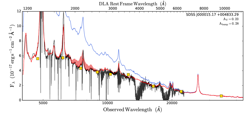
Figure 18: Combined 1D X-Shooter spectrum of J0000$+$0048 in black. The data has been replaced by the continuum over the ${\rm Ly}\,\alpha$ forest. The yellow squares indicate the photometry in $u$, $g$, $r$, $i$, $z$, $Y$, $J$, $H$, $K$, and $W1$ bands (left to right). The uncertainty on the photometry is smaller than the extent of the square marker. The blue line shows the unreddened, smoothed template by Selsing et al. (2016), and the red line indicates the same template reddened by the best-fit extinction curve by an amount of $A_{V}=0.23$. The red shaded area marks the strength of the 2175 Å bump. The upper edge of the shaded region corresponds to an extinction curve with no 2175 Å bump.

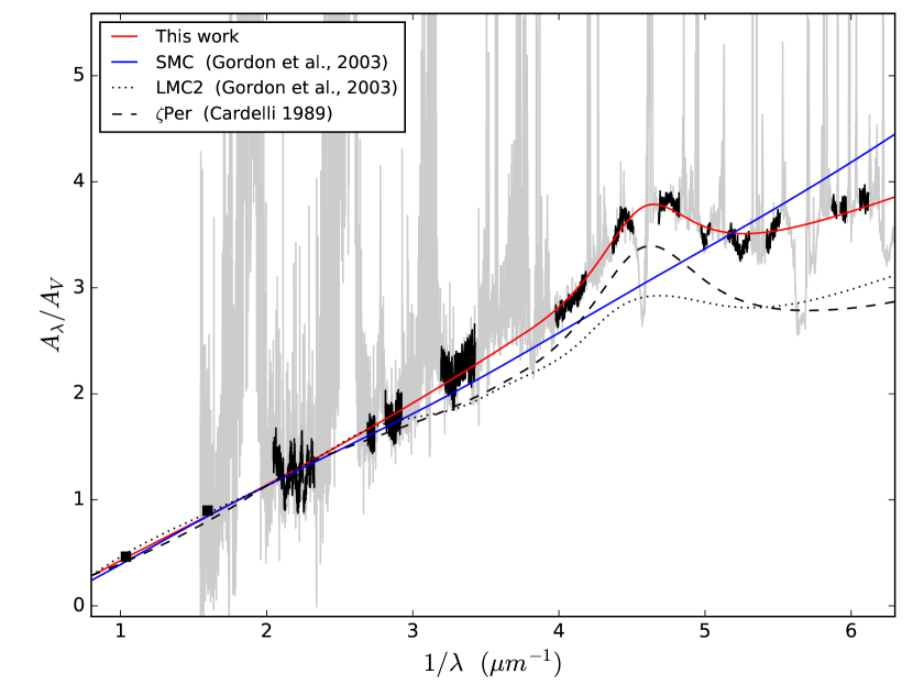
Figure 19: Extinction curve as function of inverse wavelength at the rest-frame of the DLA normalised to the $V$-band extinction $A_{V}$. The gray line shows the full X-Shooter spectrum divided by the template of Selsing et al. (2016). The black regions indicate the wavelength regions used in the fit, and the two black squares indicated the photometry in the $K$ and $W1$ bands. The red, solid line shows the best fit extinction curve, a clear 2175 Å bump is observed in the data. For comparison, the extinction curves from Gordon et al. (2003) are shown as solid blue (SMC), and gray dotted (LMC2) lines. The dashed line corresponds to a Milky-Way extinction law with the single parameter, $R_{V}$, corresponding to $\zeta$Per (Cardelli et al., 1989). A full derivation of the extinction curve towards this star is not available.

The uncertainty quoted on the $A_{V}$ from the best fit only includes the formal statistical error. This error is not fully representative as it does not take into account the intrinsic variations of the UV slope of the quasar. The slope of the quasar might vary with respect to the used template spectrum, which would lead us to infer a wrong amount of extinction. We have estimated this systematic effect on our best-fit $A_{V}$ by varying the slope of the used quasar template, by multiplying the template with a power-law normalized at 5500 Å. We note that this approach is only a rough approximation since the quasar shape is poorly described by a single power-law at all wavelengths. However, from about 1200 Å to 1 $\mu$m in the quasar rest-frame, this is a reasonable approximation. For each variation in the intrinsic slope, we fit the data again. In this fitting procedure, we keep the extinction curve parameters fixed, since varying the intrinsic slope and $R_{V}$ simultaneously leads to a completely degenerate fit with non-physical fit parameters.

For a shallower slope (by +0.2 dex), we obtain a best-fit $A_{V}$ of 0.12 mag. Conversely, for a steeper slope (smaller by $-$0.2 dex), we recover a larger best-fit value of $A_{V}$=0.34 mag. This change in slope is consistent with the average spread of intrinsic slopes observed in the literature (Vanden Berk et al., 2001; Krawczyk et al., 2015). Although the different slopes provide acceptable fits to the data, the best fit is obtained with the original quasar template.

As mentioned above, changing the slope of the template will inevitably change the slope of the recovered extinction curve. Although we cannot fit these two quantities together, we can require the fit to reproduce a value of $R_{V}$ consistent with an average Milky Way sight-line ($R_{V}=3.1$), which is obtained for a change in slope of +0.04 dex, which in return yields a best-fit $A_{V}$ of 0.17 mag.

6 Modelling of the physical conditions in the cold cloud

In this section, we aim at understanding the structure of the cold gas by modelling the physical conditions using the version c13 of the spectral simulation code Cloudy (last described in Ferland et al., 2013). This code performs a self-consistent calculation of the thermal, ionisation and chemical balance of both the gas and dust exposed to a radiation source, with a full treatment of H₂ introduced by Shaw et al. (2005). The cloud is assumed to be old enough for all physical processes to be in steady state.

6.1 Geometry and turbulence

We consider a plane-parallel geometry with radiation illuminating both surfaces of the cloud. Such geometry has been succesfully used to reproduce the physical conditions in typical interstellar clouds (e.g. van Dishoeck & Black, 1986). We consider constant density models and stop the calculation when reaching the observed H₂ column density (instead of $N({H\textsc{i}})$ whose measurement encompasses the whole profile). While H₂ is also likely present in more than one component, most of it should be found in the main cold component in which CO is also found. We consider a turbulent broadening of 0.7 ${\rm km\,s^{-1}}$, as derived from the Doppler parameter of heavy elements, see Fig. 16. This is mostly important for its effect on the CO self-shielding with a negligible effect on H₂ due to the strong damping wings.

6.2 Incident radiation field and cosmic rays

The Haardt-Madau ionising UV background from both galaxies and quasar (see Haardt & Madau, 2012) is included at the absorber’s redshift, and so is the CMB radiation. We also consider the presence of a local source of UV radiation by adding a blackbody radiation with a temperature of $T=40\,000$ K, to simulate the presence of hot stars. We parametrise the intensity of this blackbody radiation by $\chi$, the ratio of the assumed incident blackbody radiation to the Habing (1968) field (compared in the range 0.44 to 1 Ryd). Since we aim at understanding primarily the conditions in the cold cloud, we take into account the attenuation of the incident radiation after it went through neutral gas, removing photons between 1 to 4 Ryd. Cosmic rays are also included as they play a major role inside molecular regions, becoming the main source of ionisation and impacting the ion-molecule chemistry in the cold gas. Indeed, the cosmic ray ionisation rate, $\zeta_{\rm H}$, is generally deduced from the abundance of chemical ions in our own Galaxy, where it is also found to vary by a large amount between different regions (e.g. Federman et al., 1996). We note however that this remains an active area of research, with more recent studies pointing towards an average Galactic value one order of magnitude higher than previously found (see e.g. Indriolo et al., 2007).

6.3 Abundances

We set the metal abundances to 2.5 times Solar, as derived from the abundance of undepleted zinc, and assume intrinsic Solar ratio for all species. We apply the observed depletion factor for iron and silicon, which are observed in their dominant ionisation stages. Since we have no measurement of the total abundance of other species, we apply the default depletion values for the cold medium in the Galactic disc as compiled in Table 7.7 of the Hazy1 documentation of Cloudy.

6.4 Model with standard Galactic grains

As a first test, we start modelling the cloud using a canonical Milky-Way ISM dust grain mixture, with an abundance scaled to the metallicity, i.e. we set the dust grain abundance 2.5 times the Galactic ISM value. Instead of running large grids of parameters, we vary the main input parameters individually and study their effect on the predicted column densities. These parameters are: total hydrogen volumic density ($n_{H}$), strength of UV field ($\chi$) and cosmic ray ionisation rate $\zeta_{\rm H}$.

The initial density is mostly determined by matching the observed relative population of the C i fine structure level with the computed ionisation, chemical and thermal balance. Note that the density of different colliders is calculated self-consistently across the cloud. We find that densities in the range 40-100 cm^-3 predicts C i ratios consistent with the observed ones. In turn, the CO/C i ratio is strongly underpredicted by a factor of about 30. This issue was also raised by Sonnentrucker et al. (2007), who noted that most published models of translucent clouds predict less CO than observed for a given $N($H${}_{2})$. We find that decreasing $\chi$ does not help (as similarly concluded by Bensch 2006 when modelling the emission from the dark cloud Barnard 5 in the Perseus complex). Shaw et al. (2008) showed that the CO column density increases almost linearly with $\zeta_{\rm H}$, but increasing $N($CO) this way leads to a strong overproduction of C i. We therefore have to re-evaluate our initial assumptions but find that varying other parameters such as the shape of the incident UV field or the geometry of the cloud does not help either.

6.5 Model with small dust grains

Interestingly, the abundances of most molecular and neutral species observed at $z_{\rm abs}=2.5$ towards J0000$+$0048 are very similar to those observed in the Perseus cloud along $\zeta$Per, that was successfully modelled by Shaw et al. (2008). These authors used a higher number of small grains compared to a standard mixture to approximate the observed $R_{\rm V}$ and $E(B-V)$. The $\zeta$Per extinction curve is also quite similar to that observed towards J0000$+$0048, although the latter has a steeper UV slope, probably indicating a smaller average grain size. Small grains seems indeed to be a key ingredient to increase the column density of CO with respect to that of carbon and molecular hydrogen. In other words, a higher total surface of grains favors CO without going too deep into the cloud. Shaw et al. (2016) also highlighted the need of increased grain surface area to reproduce the CO column density towards SDSS J1439$+$1117 (Srianand et al., 2008).

We therefore move to a second series of models, using a dust grains size distribution containing more small grains. Typically, the distribution for each grain type (graphite and silicates) is parametrised as a single power law with the form $dn/da\propto a^{-q}$, where $n$ is the number of grains with radius in the range [$a$,$a+da$]. Nozawa & Fukugita (2013) have shown that a graphite-silicate model can reproduce well the range of extinction curves seen in the Milky-Way and Small Magellanic Cloud with a remarkably constant power law index $q\approx 3.5\pm 0.2$, with a cutoff at small ($a_{min}\sim 0.05$ $\mu$m) and large ($a_{max}\sim 0.2-0.3$ $\mu$m) grain radii. These authors note that they could not determine well the small grain cutoff due to lack of data a short wavelengths, but that these have little effect on other parameters anyway. We fixed $q=3.5$ and find that a silicate-graphite mixture with a silicate-to-graphite ratio increased by 40% compared to canonical ISM mixture, $a_{min}=0.001$ $\mu$m and $a_{max}=0.15$ $\mu$m for both grain types reproduces well the extinction curve derived in Sect. 5. In addition, we verified that the abundances of different metals locked into the grains are consistent with the observed metallicity for the assumed depletion pattern to within 0.1 dex, or better.

Using the small-grains model, we are able to reproduce most of the column densities to within 0.4 dex or better for most neutral, ionised, and molecular species, see Table 9, for $\chi=0.5$ and $\zeta_{\rm H}=2.5\times 10^{-15}$ s^-1 (Table 8). The column densities of Mg i remain however overpredicted by about 0.8 and the high rotational levels of H₂ are underpredicted. It is likely that the actual depletion of magnesium is much higher than assumed here (see De Cia et al., 2016). Indeed, for the high volumic density and molecular fraction estimated here, we can expect an order of magnitude stronger depletion of magnesium (see Jensen & Snow, 2007), in which case the model perfectly matches the observations. Finally, most of the column density in the high-$J$ levels of H₂ could arise mostly from an additional warmer component, which is not modelled here. We also note that the predicted visual extinction ($A_{V}\sim 0.7$) is higher than what we derived through SED fitting or seen towards $\zeta$Per, but within a reasonable factor, given the uncertainties on the measurement and on the intrinsic quasar brightness.

In conclusion, it is remarkable that our model reproduces fairly well the observed quantities with the small number of parameters considered. Further fine-tuning of the parameters could still be performed, and other parameters previously fixed could be varied. For example, a harder UV flux, with black-body temperature of $T\sim 60\,000$ K increases the CO column density by about 0.07 dex (hence a better agreement) while changing little the other predicted values. However, such fine-tuning is not the purpose of this paper, given the other uncertainties (in particular on the metallicity) and assumptions involved. We also remind that the true geometry of the cloud and its density profile is likely more complex than assumed. Lastly, we note that the chemistry of CO is an evolving research field. At the low densities of the ISM, CO can be formed through different paths and sequences of reaction. For example, radiative association between C⁺ and H₂ (or with a much lower efficiency with H⁰) leads to CH⁺, which then reacts with O to produce CO. Several chemistry networds (such as hydrogen-oxygen) are initiated by cosmic rays, hence their importance in controlling the production of CO. However, as discussed by Goldsmith (2013), other physical phenomena can also raise the temperature of the gas, leading to an increase of CO abundance, such as shock heating (Elitzur & Watson, 1978) or Alfvén waves (e.g. Federman et al., 1996; Visser et al., 2009). Finally, dissipation of energy from supersonic turbulence can deeply modify the chemistry of the gas (Godard et al., 2009).

Table 8: Cloudy input parameters

Parameter	Value
$n_{\rm H}$	80 cm-3
$\zeta_{\rm H}$	2.5$\times 10^{-15}$ s-1
$\chi$	0.5
turbulence	0.7 ${\rm km\,s^{-1}}$
Metallicity	2.5 $Z_{\rm\odot}$
$\log{\rm(C/H)}$	-3.57
$\log{\rm(O/H)}$	-3.13
$\log{\rm(Na/H)}$	-6.06
$\log{\rm(Mg/H)}$	-4.70
$\log{\rm(Si/H)}$	-5.49
$\log{\rm(Cl/H)}$	-6.50
$\log{\rm(Fe/H)}$	-6.50
$\log{\rm(Ni/H)}$	-7.38

Table 9: Comparison of observed and predicted values in the cold component

Quantity	observed value	model prediction
H i	$<20.9$	20.7
CO	14.95$\pm$0.05	14.72
C i	16.22$\pm$0.07	16.40
C i,$J=0$	16.10$\pm$0.08	16.19
C i,$J=1$	15.54$\pm$0.14	15.93
C i,$J=2$	14.67$\pm$0.11	15.04
S i	14.85$\pm$0.18	14.53
Cl i	14.63$\pm$0.29	14.50
Mg i	14.10$\pm$0.10	14.92
Na i	15.00$\pm$0.30	14.51
$T_{\rm 01}$ (K)	51$\pm$2	56

6.6 Characteristics of the cloud

The top panel of Fig. 20 shows the abundances of neutral atomic hydrogen, molecular hydrogen, neutral chlorine and carbon monoxide relative to the total amount of hydrogen as a function of the depth into the cloud. Only half of the profile is shown, the other half being symmetric with the assumed geometry. We find a total cloud size to be about 4 pc along the line of sight. The line of sight passes quickly through a sharp H i-to-H₂ transition, which is very well traced by neutral chlorine and after which the H₂ molecular fraction stays constant at about 50%. This incomplete conversion is due to destruction of H₂ in the cloud center, inside the self-shielding layer (see also Liszt, 2015). The abundance of CO starts to be significant immediately after the H i-to-H₂ transition. Indeed the chemical networks leading to the formation of CO with H₂ as starting point are much more efficient than those starting with atomic hydrogen (see Goldsmith, 2013). In addition, H₂ participates in the shielding of CO, through a few but important overlaps with FUV CO electronic bands (e.g. Glassgold et al., 1985; van Dishoeck & Black, 1988; Bensch, 2006; Visser et al., 2009). The abundance of C i does not vary much inside the molecular cloud, and do not directly follow H₂ nor CO. This is due to the abundance of C i being mostly determined by the ionisation/recombination balance. In addition, neutral carbon does neither benefit from H₂ shielding nor participate directly in the molecules chemistry (which rather involve C⁺). The fact that C i is considered a tracer for H₂ is therefore more indirect: C i probes the conditions that favors the presence of H₂, without locally following the latter within layers of a given molecular cloud.

The temperature (central panel) varies slowly between $\sim$ 70-80 K and 48 K towards the center of the cloud, in agreement with the average temperature measured from the column densities in the first H₂ rotational levels. Indeed, we predict T${}_{\rm 01}\sim 56$ K, very close to the measured value. Photoelectric effect on dust grains is the main heating source in the external layers on the cloud while cosmic rays become the main heating source in the cloud center. Heating by H₂ photo-dissociation contributes for a small fraction to the total heating and naturally decreases after the H i-to-H₂ transition. Cooling is in turn largely dominated by [C ii]$157\mu$m emission. The model predicts $\log N({C\textsc{ii}}^{*})=15.64$. Unfortunately, we cannot test this prediction since the measurement is affected by a large uncertainty.

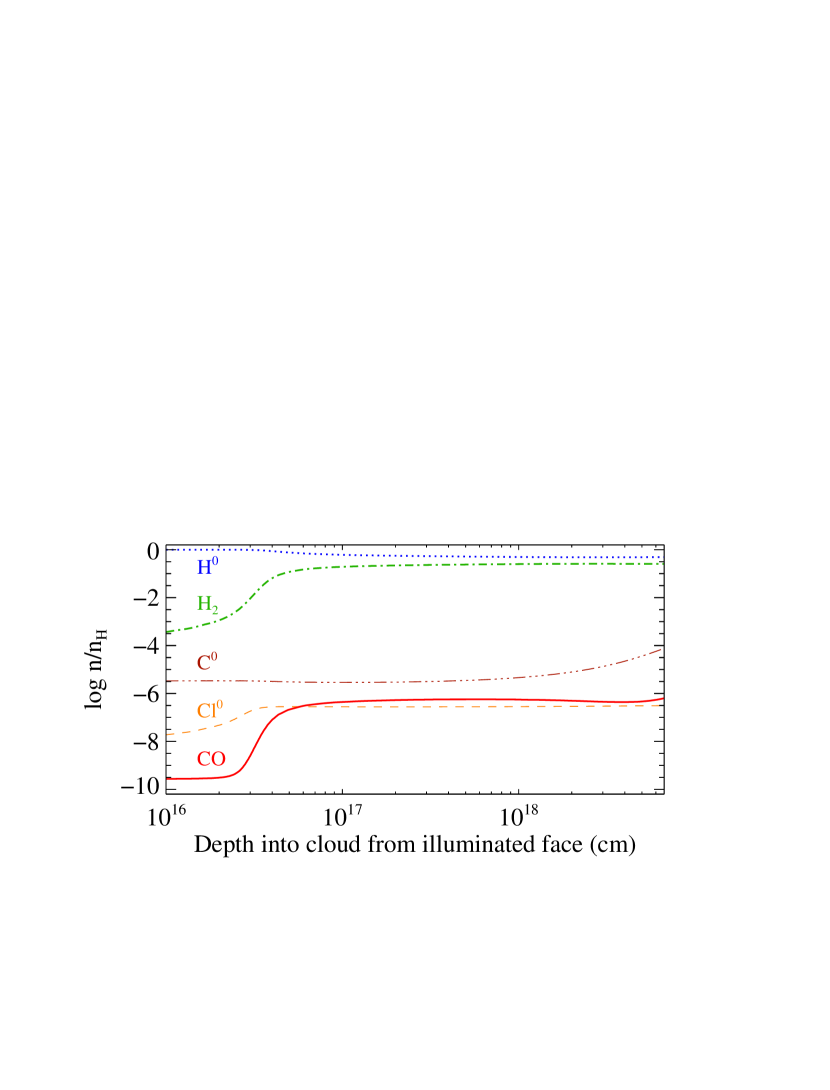
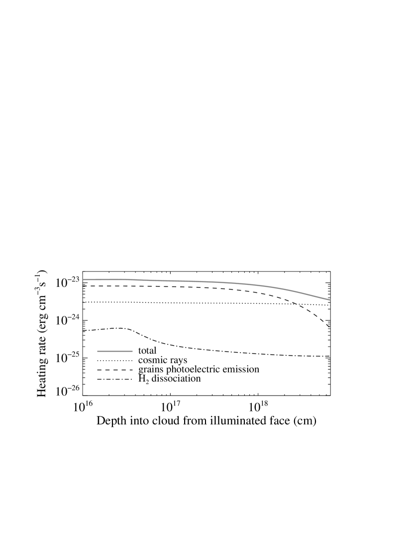
Figure 20: Top panel: variation of the abundances of neutral atomic hydrogen (blue dotted), molecular hydrogen (green dashed-dotted), neutral chlorine (orange dashed) neutral carbon (brown, dashed-triple dotted) and carbon monoxide (red) as a function of depth into the cloud. Note that for H₂, the curve corresponds to half the molecular fraction (since $f=2n_{\rm H2}/n_{\rm H}$). Middle panel: Variation of the temperature across the cloud. Bottom panel: Heating rates for the main sources. The cooling rate, which is largely dominated by [C ii]$157\mu$m emission, equals the total heating rate since the cloud is assumed in thermal equilibrium.

7 Temperature of the Cosmic Microwave Background at $z=2.53$

Srianand et al. (2008) and Noterdaeme et al. (2011) have shown that the excitation of CO at high redshift is largely dominated by the CMB radiation, i.e., that other excitation processes such as collision are negligible, in which case $T_{\rm ex}($CO$)\approx T_{\rm CMB}$. More recently, Sobolev et al. (2015) estimated a correction to apply if we do take into account collisional excitation with hydrogen atoms and H₂ molecules. The correction depends almost linearly on the total volumic density and on the kinetic temprature. In addition, since the main collision partner is H₂, the correction increases with the molecular fraction. Using $f=0.5$, $T=50$ K and $n_{\rm H}=80$ ${\rm cm}^{-2}$, their Eq. 7 implies an excess temperature of $\Delta T=$ 0.3 K. Applying this correction to the observed CO excitation temperature towards J0000$+$0048 ($T_{\rm ex}($CO$)=9.9^{+0.7}_{-0.6}$ K, see Fig. 21) we obtain $T_{\rm CMB}(z=2.53)=9.6^{+0.7}_{-0.6}$ K in excellent agreement with the expected CMB temperature in the standard hot Big-Bang theory ($T_{\rm CMB}=T_{0}(1+z)=9.61$ K). Using the statistical equilibrium radiative transfer code RADEX (van der Tak et al., 2007), that takes as input the density of various colliders, the kinetic temperature, CO Doppler parameter and column density, we also obtain very similar results, within 0.1 K. We finally remind that since the expected excess temperature is almost linearly dependent on the both kinetic temperature and the density, good constraints on these quantities are highly valuable.

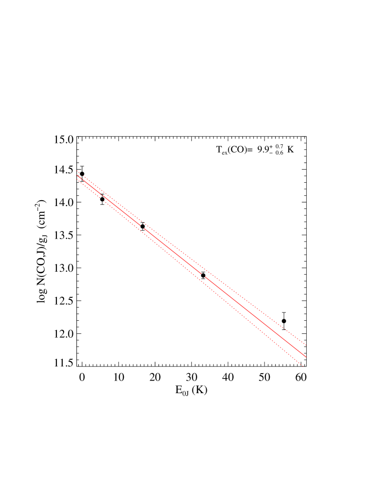
Figure 21: CO excitation diagram. The solid line gives the best fit to the rotational population using a Boltzmann distribution, with the associated uncertainty shown as dashed line.

Our Cloudy model predicts $T_{\rm ex}($CO$)=10$ K when the expected CMB radiation field at $z=2.53$ is included, in agreement with the observed temperature. To test further the effect of the CMB radiation, we run a model setting the CMB background temperature to the value measured at $z=0$ instead ($T_{0}=2.726$ K, Fixsen, 2009), while keeping all other parameters the same as previously. This model predicts a CO excitation temperature of 3.8 K, that we derive from the predicted population of the first three rotational levels since higher rotational levels do not follow the Boltzmann distribution anymore. The predicted temperature would then be similar to that seen in diffuse Galactic environments (Burgh et al., 2007) but about 10$\sigma$ away from the measured value towards J0000$+$0048. We also note that the difference between CMB temperature and CO excitation temperature tends to vanish at high redshift, where excitation by CMB becomes strongly dominant over collisional excitation.

Our result suggests ways to improve the constraints on the evolution of the CMB temperature at high redshift. From the distribution of the CO rotational levels alone, any departure from the Boltzmann distribution will be due to non-CMB (presumably collisionnal) processes. This means that a measurement remains possible using the low rotational levels, as in Noterdaeme et al. (2010). However, a good understanding of the physical conditions in the cloud, and in particular the temperature and density – that can be very effectively constrained by the observations of low-$J$ H₂ lines and C i fine-structure levels– allows one to correct for collisional excitation. The excess temperature for diffuse molecular cloud will typically be of the order of 0.3 K, i.e. a few times larger than the expected measurement uncertainty achievable with future high resolution spectographs on extremely large telescopes. This will therefore need to be carefully evaluated.

Cyanogen (CN) is known to be an even better thermometer of the CMB temperature, with negligible contribution from collisions. Very accurate measurements have been performed using absorption spectroscopy towards nearby stars, including observations towards $\zeta$Per (e.g. Roth & Meyer, 1995; Ritchey et al., 2011). The similarity with our line of sight provides a good hope that CN lines will also be detectable in systems like J0000$+$0048. Indeed, a strong correlation between $N($CO) and $N($CN) is observed in our Galaxy (e.g. Fig. 18 of Sonnentrucker et al., 2007), with $N$(CN) of a few times 10¹² ${\rm cm}^{-2}$ at the CO column density of our system. However, obtaining high S/N and resolution in the NIR where the CN$\lambda$3875 lines are redshifted is technically challenging. In the case of J0000$+$0048, the lines unfortunately fall in a region of low transmission due to water vapour in the atmosphere. This means that the search for similar molecular systems at higher redshift (e.g. $z\sim 2.9-3.5$ for the CN lines to be redshifted in the H-band) needs to be continued. The CMB contribution for such systems will also be higher and their constraint on the evolution of CMB temperature stronger.

8 Direct search for star-formation activity

Motivated by the similarity between this absorbing cloud and the local ISM, we search for the emission associated with active star formation. The main indicator of star formation, available to us in the data at hand, is the nebular emission lines from the photo-ionised gas in the vicinity of young stars. The most prominent of these lines in the rest-frame UV and optical are the two principal Balmer lines (H$\alpha$ and H$\beta$) and the two doublets from singly and doubly ionised oxygen ([O ii]$\lambda\lambda$3726,3728 and [O iii] $\lambda\lambda$ 4959, 5007), which at the redshift of the DLA fall in the NIR spectrum from X-Shooter. Unfortunately the H$\alpha$ line falls in the last order of the NIR spectrum, which is corrupted by strong sky background. We therefore search for emission from the DLA counterpart using the following lines: H$\beta$, [O iii], and [O ii]. However, we do not detect emission from any of the lines.

For each PA, we first subtract the quasar trace in the 2D spectrum using a similar approach as described in Krogager et al. (2013) in order to search for the faint emission lines. In the following, we have combined the observations taken with a same position angle.

We use an elliptical extraction aperture to search for the lines. In the spatial direction, we use a semi-minor axis extent of one full width at half maximum of the spectral trace (FWHM = 5 pixels). In the spectral direction, we use a semi-major axis of $400$ km s^-1 around the expected location given from the redshift of the DLA. However, we observe no flux in any of the PAs. We derived the detection limit for the [O ii] line by modelling 10 000 emission line profiles with various line fluxes (drawn randomly in log-space between $1\times 10^{-18}$ and $1\times 10^{-16}\leavevmode\nobreak\ {\rm erg}\leavevmode\nobreak\ {\rm s}^{-1}\leavevmode\nobreak\ {\rm cm}^{-2}$), line widths (drawn randomly between 50 and 350 km s^-1), and line strength ratio for the two transitions of the doublet (randomly drawn between 0.35 and 1.5; see Seaton & Osterbrock, 1957). Each model line profile (assumed to be Gaussian) is convolved with the spatial broadening function, determined from the spatial profile of the quasar trace, to create a 2D line model. We subsequently add noise to the 2D line model according to the noise model from the 2D spectrum. For each realisation, we extract the flux and noise within the elliptical aperture mentioned above. This results in a robust limit on the detectable flux within the aperture, given the fact that we do not know the intrinsic line width of the [O ii] line. We quote all the non-detections for the individual PAs as 3$\sigma$ upper limits in Table 10.

Due to the nodding strategy used for the X-Shooter observations, only the central $6.4\arcsec$ (out of the total $11\arcsec$ slit length) are suitable for the analysis. However, in the overlap of all the slits, we are able to combine the individual limits to improve the constraint on the line flux. We combine the individual 2D spectra to look at emission but recover no detection. Using the same elliptical aperture as mentioned above, we measure a 3$\sigma$ limit consistent with the value obtained from the combination of the 4 individual limits. The combined limit measured in the combined stack of all spectra is given in the last row of Table 10. This central region roughly corresponds to a circular aperture with a 1.2 arcsec diameter, which at the redshift of the DLA translates to 5.0 kpc. The configuration of slits is shown in the schematic map of exposure time in Figure 22.

We can use the constraint on the line flux of [O ii]$\lambda$3727 to put a limit on the star formation rate. Instead of using the relation from Kennicutt (1998), which is calibrated using local galaxies, we use the empirical dust-uncorrected $L[{O\textsc{ii}}]-$SFR relation from Krühler et al. (2015). This relation was constructed using high redshift GRB-DLA host galaxies and implicitely accounts for dependence on galactic properties (e.g. Kewley et al., 2004). The inferred star formation rates are summarised along with the flux limits in Table 10.

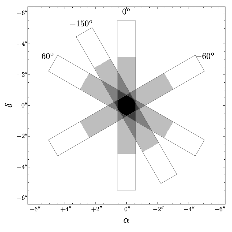
Figure 22: The positions of the X-Shooter slits on the sky relative to the quasar position. The thin gray lines indicate the full X-Shooter slit length (11 arcsec). The colour coding indicates effective exposure time in the part of the slit available to our analysis (see text): darker colour corresponds to higher exposure time. For each slit position, the position angle is given at the end of the slit.

Table 10: Limits on star-formation rate from the non-detection of [O ii].

PA	$F([{O\textsc{ii}}])$	SFR
(deg)	($10^{17}$ erg s-1 cm-2)	(M⊙ yr-1)
0	$<$ 4.0	$<$ 22
-150	$<$ 3.0	$<$ 16
-60	$<$ 3.8	$<$ 21
+60	$<$ 4.3	$<$ 24
combined	$<$ 1.9	$<$ 9.9

9 Summary

In this work, we present the detection and detailed analysis of an exceptional molecular absorber at $z_{\rm abs}=2.53$ towards the quasar J0000$+$0048, being one of the very few absorption systems featuring CO absorption lines known to date (see Noterdaeme et al. 2011 and references therein, Ma et al. 2015). Using both high resolution and multiwavelength spectroscopic observations, we derive the chemical composition, dust depletion and extinction as well as the molecular content of this cloud. Our main findings are the following:

(1) The absorption system is characterised by super-Solar metallicity (about 2.5 $Z_{\rm\odot}$). Although the uncertainty on this value is large (by a factor of about 2-3), it is much higher than the metallicities seen in the overall population of H i-selected DLAs at this redshift (see e.g. Rafelski et al., 2012). The observed depletion of refractory elements is typical of cold gas in the Galactic disc and peaks at the location where molecular gas is found. Higher spectral resolution data would be desirable to constrain better the amount of metals in this very narrow component ($b\sim$0.7 ${\rm km\,s^{-1}}$).

(2) The DLA has a molecular fraction reaching almost 50% overall, being the largest value measured till now in a high-$z$ absorption system, for a total neutral hydrogen column density of $\log N({\rm H})=20.8$. This corresponds to a neutral gas surface density of $\Sigma_{\rm HI}\approx 5$ M_⊙ pc^-2 and a molecular hydrogen surface density $\Sigma_{\rm HI}\approx 4.4$ M_⊙ pc^-2. These surface densities are very similar to what is seen across the Perseus molecular cloud from high spatial resolution emission observations (Lee et al., 2012), despite the H i and H₂ surface densities being measured directly along a pencil beam line of sight in our study while derived from dust maps in the latter. This also shows that H i-to-H₂ transition in our high-$z$ system is likely following the same physical processes as in our Galaxy.

(3) We further use the different molecular and atomic species to constrain the actual physical conditions in the cold gas with the help of the spectral synthesis code Cloudy. We find that the column densities can be well reproduced by a cloud with density around $n_{\rm H}\sim 80$ cm^-3 inmersed into a moderate UV field, similar to the local interstellar radiation field. We show that a high cosmic ray ionisation rate together with the presence of small dust grains – consistent with the depletion pattern, the steep extinction curve, and presence of a 2175 Å bump – can explain the high CO fractional abundance. The model also predicts a kinetic temperature around 50 K, in perfect agreement with that derived from the excitation of H₂. The CO abundance rises immediately after the H i-to-H₂ transition, thanks to the efficient chemistry paths involving H₂, together with pre-shielding of CO. About half of the hydrogen remains in atomic form in the cloud interior, well inside the H i-to-H₂ transition layer, due to H₂ destruction by cosmic rays. This can also explain the high HD/2H₂ ratio through chemical enhancement of HD compared to H₂. We must however keep in mind that, in addition to cosmic rays, several other processes heating the gas can also enhance the production of CO (Goldsmith, 2013) and that our model suffers from uncertainties in several imput parameters, such as the metallicity. The detection of more molecular species in this system, together with comparison of different codes (e.g. the Meudon PDR code, Le Petit et al., 2006) should break degeneracies between parameters such as dust abundance and cosmic ray rate and lead to a better understanding of the physical processes at play. Our study suggests that the presence of strong C i lines, detectable at low spectral resolution (as in Ledoux et al., 2015), is a good indicator for high molecular hydrogen column density (in self-shielded regime), but this (or directly detecting damped H₂ lines as in Balashev et al. 2014) is not a sufficient condition to get CO in detectable amounts. Since small grains seem to play a crucial role in the production of CO, selecting systems that, in addition to C i, also present a steep extinction curve and/or the presence of a 2175 Å bump should significantly increase the probability to detect CO.

(4) While our study shows that the line of sight towards J0000$+$0048 has chemical and physical characteristics similar to those found in diffuse molecular regions of the Perseus cloud, we show that the former absorbing cloud is immersed into a warmer cosmic microwave background radiation. We derive the temperature of the CMB radiation at the absorber’s redshift from the excitation of CO lines, correcting for a small temperature excess due to collisional excitation. The temperature we obtain is in perfect agreement with the adiabatic cooling expected in the standard hot Big-Bang theory, $T_{\rm CMB}(z)=T_{0}\times(1+z)\approx 9.6$ K at $z=2.53$.

Final remarks: The discovery presented here was facilitated by the steadily increasing number of available spectra of faint quasars, together with sensitive instruments on large telescopes. The involved amounts of carbon monoxide remain however far too low to be detectable in emission (even if it were at $z=0$), making the cloud being an example of CO-dark molecular gas (Wolfire et al., 2010). Interestingly, such furtive phase may actually contain a large fraction of the total molecular gas in galaxies (e.g. Smith et al., 2014). Efforts should therefore be pursued to detect more absorption systems like the one presented here at high-redshift. These will provide excellent targets for detailled high-resolution studies (including CMB temperature) using the next generation of extremely large telescopes.

Appendix A Robustness of the CO measurement

When estimating best-fit parameters, vpfit takes as input the normalised spectrum and the resolution provided by the user. This means that continuum placement uncertainties and errors due to the knowledge of the spectral point spread function (SPSF) are not reflected in the error estimates.

We test the effect of SPSF uncertainties by refitting the data, using a range of spectral resolution from 4.75 to 5.25 ${\rm km\,s^{-1}}$. The resulting parameters remain well within their associated fitting uncertainty, with total column density varying by only $\pm$0.05 dex, excitation temperature (see Fig. 21) varying by $\Delta T_{\rm ex}\sim 0.1$ K and Doppler parameter basically unchanged ($<$2%). We also fitted the two red spectra simultaneously, instead of combining them (Fig. 23). The results are also very close to what we get from the combined spectrum, as can be seen from the blue and red error bars on Fig. 24, with a slight improvement in the $\chi^{2}_{\nu}=1.03$ probably thanks to the better evaluated SPSF.

To estimate the effect of continuum placement uncertainties, we independently renormalised each region around CO absorption bands by randomly modifying the local continuum slope and intercept, following their respective normal error distribution. The distribution of CO column densities, Doppler parameter and excitation temperature obtained for hundred realisations of this “shaky” continuum procedure is shown on Fig. 24. Clearly, the effect of continuum placement uncertainty is well within the error estimates from fitting the lines but highlights the correlation between $b$, $N$ and $T_{\rm ex}$. For example, a smaller Doppler parameter will result in a higher column density and a lower excitation temperature. It can also be seen from this figure that the most deviant points generally also have the highest $\chi^{2}_{\nu}$-values.

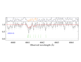
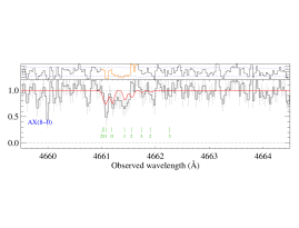
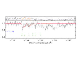
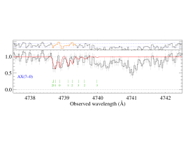
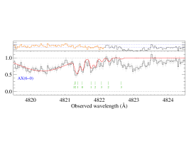
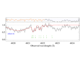
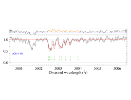
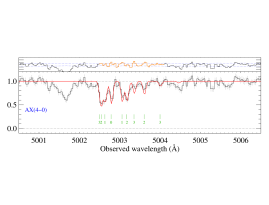
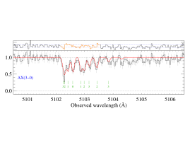
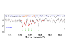
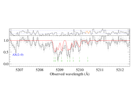
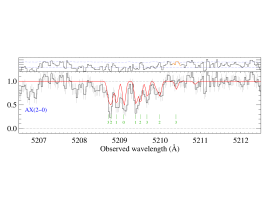
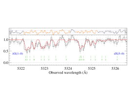
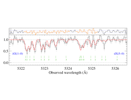
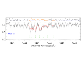
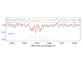
Figure 23: Voigt-profile fit to the CO absorption bands, labelled in blue in each panel. The left (resp. right) panels correspond to data taken with the 0.9” (resp. 0.7”) slit. Rotational levels from $J=0$ to $J=3$ are indicated as green tick marks. The panel above each region shows the residual, with the blue line indicating the $\pm$1 $\sigma$ interval, and the orange regions that used to constrain the fit.

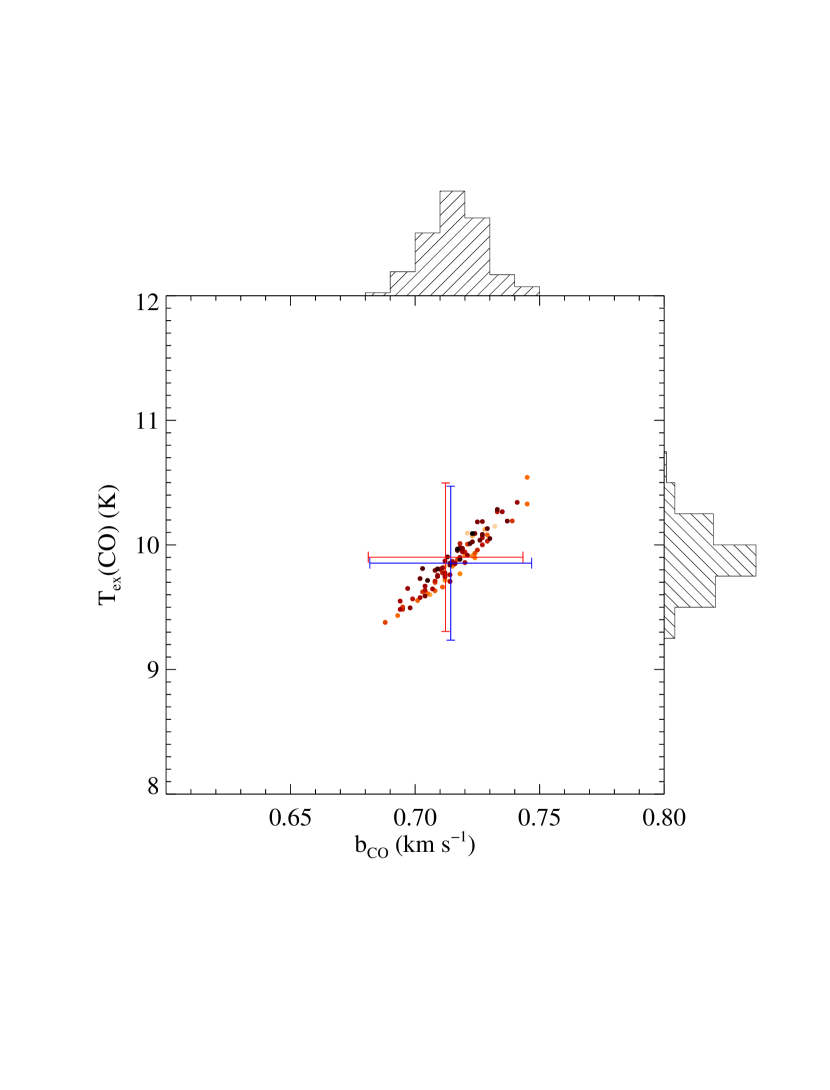
Figure 24: Effect of continuum placement uncertainties on the total CO column density, excitation temperature and Doppler parameter. The histograms represent the distributions of $\log N($CO), $T_{\rm ex}$(CO) and $b$ for 100 realisations where the continuum for each fitting region has been modified independently and randomly. The colour of each point indicates the reduced $\chi^{2}$ that varies from 1.08 (darkest) to 1.23 (lightest). The blue (resp. red) error bar corresponds to the best fit value using the combined UVES spectrum (resp. both UVES spectra fitted simultaneously).