Landau-Zener-Stueckelberg physics with a singular continuum of states

Abstract

This work addresses the dynamical quantum problem of a driven discrete energy level coupled to a semi-infinite continuum whose density of states has a square-root-type singularity, such as states of a free particle in one dimension or quasiparticle states in a BCS superconductor. The system dynamics is strongly affected by the quantum-mechanical repulsion between the discrete level and the singularity, which gives rise to a bound state, suppresses the decay into the continuum, and can produce Stueckelberg oscillations. This quantum coherence effect may limit the performance of mesoscopic superconducting devices, such as quantum electron turnstile.

Landau-Zener (LZ) transition between two coupled quantum states whose energies cross in time is a paradigmatic situation in quantum mechanics. Due to its generality and simplicity, the LZ model, originally proposed to describe atomic collisions Landau (1932); Zener (1932); Stueckelberg (1932) and spin dynamics in a magnetic field Majorana (1932), was later applied to many different phenomena, such as electron transfer in donor-acceptor complexes May and Kuhn (2000), spin dynamics in magnetic molecular clusters Wernsdorfer and Sessoli (1999), molecular production in cold atomic gases Sun et al. (2008), electron pumping Renzoni and Brandes (2001) and capture Kashcheyevs and Timoshenko (2012) in quantum dots, dissipation in driven mesoscopic rings Gefen and Thouless (1987) or in superconductor tunnel junctions Schön and Zaikin (1990); Weißl et al. (2015). In the course of intense research in various fields, several generalizations of the two-level LZ model to multiple levels have been found Demkov and Osherov (1968); Brundobler and Elser (1993); Demkov et al. (1995); Ostrovsky and Nakamura (1997); Demkov and Ostrovsky (2001); Pokrovsky and Sinitsyn (2002); Volkov and Ostrovsky (2004); Shytov (2004); Patra and Yuzbashyan (2015) including finite-time exact solutions Vitanov and Garraway (1996); Mkam Tchouobiap et al. (2015), and even many-body versions of the LZ model have been considered Keeling and Gurarie (2008); Altland and Gurarie (2008); Sun et al. (2008); Ishkhanyan (2010). However, these generalizations still deal with discrete energy levels. A notable exception is Ref. Demkov and Osherov (1968), whose authors analyzed a single discrete level driven linearly through an arbitrary spectrum, which could also be continuous.

In the present paper, I present another extension of the Landau-Zener problem involving a discrete level coupled to a continuum of states, which has an approximate analytical solution in the long-time limit. The continuum states are assumed to have positive energies, $E>0$, with the density of states (DOS) $\nu(E)$ having a singularity $\nu(E)\propto{1}/\sqrt{E}$ at $E\to{0}^{+}$. This singularity is the essential ingredient of the problem. Physically, such continuum can be represented by a one-dimensional wire with the parabolic dispersion, or by quasiparticle states in a BCS superconductor above the superconducting gap. The discrete level (located on an impurity or a small quantum dot) initially has large negative energy and contains one particle. Then, its energy $E_{\mathrm{d}}$ is moved inside the continuum (e. g., by applying a gate voltage), where it stays for some time, and then is driven back to large negative energies, as shown in Fig. 1 by the dashed line. The quantity of interest is the probability $p_{\infty}$ for the particle to stay on the discrete level without being ejected into the continuum. A related problem of vanishing bound state in atom-ion collisions was considered in Ref. Demkov (1964).

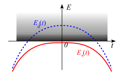
Figure 1: (Color online) A sketch of the time dependence of various energies. The grey area at $E>0$ represents the continuum with the singularity in the DOS at $E\to{0}$. The dashed blue line shows the the bare discrete level $E_{\mathrm{d}}(t)$, driven inside the continuum for a finite time. The solid red line shows the adiabatic ground state $E_{*}(t)$.

The practical motivation for the present study comes from the quantum electron turnstile, a nanoelectronic device transferring electrons one by one, with a potential metrological application as a current standard (see reviews Pekola et al. (2013); Kaestner and Kashcheyevs (2015)). The electron transfer occurs via a small metallic nanoparticle sandwiched between two superconducting electrodes Pekola et al. (2008). For a small enough particle, the electron confinement is very strong, so there is effectively a single electronic level whose double occupancy is prohibited by the Coulomb repulsion, and whose energy is controlled by a nearby gate electrode van Zanten et al. (2015, 2016). The key step of the operation is the electron ejection from the nanoparticle level, driven by the gate voltage, into the empty quasiparticle states on one of the superconducting electrodes. If the superconducting gap is large enough, one can consider the single-particle problem. The level trajectory then corresponds to that shown in Fig. 1, with the energy counted from the BCS singularity. The survival probability $p_{\infty}$ contributes to the turnstile operation error.

The standard description of the decay into a continuum is by the perturbative Fermi Golden Rule, which gives the decay rate $\Gamma(E_{\mathrm{d}})$ for a fixed level energy $E_{\mathrm{d}}$. Application of the Golden Rule at each instant of time gives

$$p_{\infty}=\exp\left[-\int_{E_{\mathrm{d}}(t)>0}\Gamma(E_{\mathrm{d}}(t))\,dt\right],$$ (1)

where the integration is over the time interval during which the level stays inside the continuum. Obviously, Eq. (1) is not valid for a too fast drive leading to a large energy uncertainty. Much less obvious is the breakdown of the quasistationary Eq. (1) at slow drive. It is the main focus of the present paper.

The key fact is that for a fixed $E_{\mathrm{d}}$, the exact eigenstates of the coupled system form a continuum at $E>0$, and in addition, there is a discrete bound state at an energy $E=E_{*}<0$ Fetter (1965); Machida and Shibata (1972); Shiba (1973), similar to Yu-Shiba-Rusinov states bound to a magnetic impurity Yu (1965); Soda et al. (1967); Shiba (1968); Rusinov (1969). For large negative $E_{\mathrm{d}}$, the bound state approximately coincides with the bare discrete level, $E_{*}\approx{E}_{\mathrm{d}}$. For $E_{\mathrm{d}}>0$, no matter how large, the bound state with $E_{*}<0$ still exists, although for $E_{\mathrm{d}}\to+\infty$ its energy approaches the continuum and its overlap with the bare discrete state vanishes. The existence of the bound state is a consequence of the DOS singularity at $E\to{0}^{+}$ and can be viewed as due to the quantum-mechanical repulsion between the bare level and the singularity. As the bound state is the adiabatic ground state of the coupled system, for slow drive the particle will always stay in it, implying $p_{\infty}\to{1}$.

To describe the crossover between the regime of Eq. (1) and the adiabatic regime with $p_{\infty}\to{1}$, one has to analyze the dynamical problem. Below, its analytical solution is presented for a special case of the parabolic time dependence $E_{\mathrm{d}}(t)$, obtained by adapting the method of Demkov and Osherov Demkov and Osherov (1968). Remarkably, the survival probabilty has the two-path structure $p_{\infty}=|A_{\mathrm{d}}+A_{*}|^{2}$, where $A_{\mathrm{d}}$ corresponds to the resonance in the continuum (the dashed line in Fig. 1) with $|A_{\mathrm{d}}|^{2}$ decaying according to Eq. (1), while the non-decaying $A_{*}$ is the contribution of the adiabatic ground state (the solid line in Fig. 1). The cross-term in $p_{\infty}$ describes Stueckelberg-like interference between the two paths, leading to an oscillatory dependence of $p_{\infty}$ on the drive parameters. Indeed, the bound state may be viewed as a result of avoided crossing between the discrete level and the singularity; the double passage of this crossing is similar to Stueckelberg interferometer.

The model. In a BCS superconductor, the quasiparticle DOS is given by $\nu(\epsilon)=\nu_{0}\,\theta(|\epsilon|-\Delta)|\epsilon|/\sqrt{\epsilon^{2}-\Delta^{2}}$, where $\nu_{0}$ is the normal-state DOS, the energy $\epsilon$ is counted from the Fermi level, $2\Delta$ is the superconducting gap, and $\theta(\epsilon)$ is the step function. In the vicinity of the BCS singularity at $\epsilon\to\Delta$, the quasiparticle energy, counted from $\Delta$ (it is convenient to shift the energy reference as $E=\epsilon-\Delta)$, can be approximated as $E_{k}=\sqrt{\xi_{k}^{2}+\Delta^{2}}-\Delta\approx\xi_{k}^{2}/(2\Delta)$, and the Bogolyubov quasiparticle factors $u_{k}\approx{v}_{k}\approx{1}/\sqrt{2}$. Here the index $k$ labels the quasiparticle states, and $\xi_{k}$ are the normal-state quasiparticle energies, so that the state summation $\sum_{k}$ is represented as $\nu_{0}\int{d}\xi_{k}$. The particle wave function has a component $\psi_{\mathrm{d}}$ on the bare discrete level, and components $\phi_{k}$ on the continuum states. They satisfy the two components of the Schrödinger equation (we set $\hbar=1$):

$$i\,\frac{d\psi_{\mathrm{d}}}{dt}=E_{\mathrm{d}}(t)\,\psi_{\mathrm{d}}+\sqrt{\frac{\gamma_{0}}{2\pi\nu_{0}}}\,\phi_{k},$$ (2)

$$i\,\frac{d\phi_{k}}{dt}=\frac{\xi_{k}^{2}}{2\Delta}\,\phi_{k}+\sqrt{\frac{\gamma_{0}}{2\pi\nu_{0}}}\,\psi_{\mathrm{d}},$$ (3)

where the coupling strength is parametrized by $2\gamma_{0}$, the energy-independent decay rate in the normal state. These equations can be equivalently rewritten in the coordinate representation, $\phi_{k}=\int\phi(x)e^{ikx}\,dx$, $\xi_{k}^{2}\to-v_{F}^{2}\partial_{x}^{2}$, where $v_{F}$ is the Fermi velocity; then they become identical to the Schrodinger equation for a simple one-dimensional wire coupled to a discrete site at $x=0$.

The exact eigenstate energies for fixed $E_{\mathrm{d}}$ are found by substituting $i(d/dt)\to{E}$ and eliminating $\phi_{k}$. This gives the equation $G_{\mathrm{d}}^{-1}(E)=0$, where the bare discrete level Green’s function and the self-energy are defined as

$$G_{\mathrm{d}}(E)=\frac{1}{E-E_{\mathrm{d}}-\Sigma(E)},\quad\Sigma(E)=-\sqrt{\frac{\gamma_{0}^{2}\Delta}{-2E}}.$$ (4)

$\Sigma(E>0)$ is imaginary, describing the particle escape from the discrete level into the continuum with the rate $\Gamma(E)=-2\mathop{\mathrm{Im}}\nolimits\Sigma(E+i0^{+})$. $\Sigma(E<0)$ is real and negative, describing the quantum-mechanical level repulsion. The divergence of $\Sigma(E\to{0}^{-})$ results in the existence of a real solution of $G_{\mathrm{d}}^{-1}(E)=0$ with $E=E_{*}<0$ for any $E_{\mathrm{d}}$. Thus, the spectrum consists of a discrete bound state at $E=E_{*}$, represented by the isolated pole of $G_{\mathrm{d}}(E)$, and of the continuum at $E>0$, corresponding to the branch cut of $\sqrt{-E}$. The weight of the bare discrete level in the exact bound state is given by the residue $Z$ of $G_{\mathrm{d}}(E)$ in the pole $E=E_{*}$. For positive $E_{\mathrm{d}}\gg(\gamma_{0}^{2}\Delta)^{1/3}$, the bound state is shallow, $E_{*}\approx-\gamma_{0}^{2}\Delta/(2E_{\mathrm{d}}^{2})$, and the weight is small, $Z\approx\gamma_{0}^{2}\Delta/E_{\mathrm{d}}^{3}$.

Knowledge of the eigenstates at fixed $E_{\mathrm{d}}$ enables one to treat a special case when the level energy abruptly rises from $-\infty$ to a finite value $E_{\mathrm{d}}$ (a quantum quench), stays constant for a long time, and then drops back to $-\infty$. The probability amplitude on the ground state after the first quench is given by the projection of the discrete level on the ground state, $\sqrt{Z}$. After a sufficient time the continuum component is dephased, so on the second quench the bound state is projected back on the discrete state, which gives another factor $\sqrt{Z}$. The resulting survival probability (amplitude squared) is then $p_{\infty}=Z^{2}$.

Returning to the dynamical problem, we eliminate $\phi_{k}(t)$ from Eqs. (2), (3), and obtain an equation for $\psi_{\mathrm{d}}(t)$,

$$i\,\frac{d\psi_{\mathrm{d}}(t)}{dt}=E_{\mathrm{d}}(t)\,\psi_{\mathrm{d}}(t)+\int_{-\infty}^{t}\tilde{\Sigma}(t-t^{\prime})\,\psi_{\mathrm{d}}(t^{\prime})\,dt^{\prime},$$ (5)

where $\tilde{\Sigma}(t)=e^{5i\pi/4}\theta(t)\sqrt{\gamma_{0}^{2}\Delta/(2\pi{t})}$ is the Fourier transform of $\Sigma(E+i0^{+})$. Equation (5) should be solved with the initial condition $|\psi_{\mathrm{d}}(t\to-\infty)|=1$, and the quantity of interest is $p_{\infty}=|\psi_{\mathrm{d}}(t\to+\infty)|^{2}$.

Markovian regime. Let us pass to the interaction representation by writing $\psi_{\mathrm{d}}(t)=\Psi_{\mathrm{d}}(t)\,e^{-i\Phi(t)}$, where $\Phi(t)\equiv\int_{0}^{t}E_{\mathrm{d}}(t^{\prime})\,dt^{\prime}$. Equation (5) becomes

$$i\,\frac{d\Psi_{\mathrm{d}}(t)}{dt}=\int_{-\infty}^{t}\tilde{\Sigma}(t-t^{\prime})\,e^{i\Phi(t)-i\Phi(t^{\prime})}\,\Psi_{\mathrm{d}}(t^{\prime})\,dt^{\prime}.$$ (6)

If $e^{i\Phi(t)-i\Phi(t^{\prime})}$ is quickly oscillating for $t^{\prime}$ far from $t$, the integral converges at short $t-t^{\prime}$. If the time dependence of $\Psi_{\mathrm{d}}(t^{\prime})$ is slow enough on the convergence time scale, one can approximate $\Psi_{\mathrm{d}}(t^{\prime})\approx\Psi_{\mathrm{d}}(t)$ and take it out of the integral (Markovian approximation). The resulting differential equation is straightforwardly integrated to give

$$p_{\infty}=\exp\left(-2\int_{0}^{\infty}\frac{dE}{2\pi}\sqrt{\frac{\gamma_{0}^{2}\Delta}{2E}}\,|F(E)|^{2}\right),$$ (7)

where $F(E)\equiv\int{e}^{iEt-i\Phi(t)}\,dt$. Equation (1) can be obtained from Eq. (7) by calculating $F(E)$ in the stationary phase approximation, or, equivalently, by approximating $\Phi(t)-\Phi(t^{\prime})\approx{E}_{\mathrm{d}}(t)(t-t^{\prime})$ in Eq. (6), whose right-hand side then becomes just $\Sigma(E_{\mathrm{d}}(t))\,\Psi_{\mathrm{d}}(t)$.

The Markovian character of the integral (6) is lost most easily at times $t\approx{t}_{0}$ when $E_{\mathrm{d}}(t_{0})=0$. Approximating $\Phi(t)\approx\Phi(t_{0})+\dot{E}_{\mathrm{d}}(t_{0})\,(t-t_{0})^{2}/2+\ddot{E}_{\mathrm{d}}(t_{0})\,(t-t_{0})^{3}/3$, where $\dot{E}_{\mathrm{d}}\equiv{d}E_{\mathrm{d}}/dt$, $\ddot{E}_{\mathrm{d}}\equiv{d}^{2}E_{\mathrm{d}}/dt^{2}$, we obtain the condition for the validity of the Markovian approximation as $\max\{|\dot{E}_{\mathrm{d}}|^{3/2},|\ddot{E}_{\mathrm{d}}|\}\gg\gamma_{0}^{2}\Delta$. If $E_{\mathrm{d}}(t)<0$ always, the validity is determined by the values $E_{\mathrm{d}}(t_{\mathrm{max}})$, $\ddot{E}_{\mathrm{d}}(t_{\mathrm{max}})$ at the maximum: $\max\{|E_{\mathrm{d}}^{3}|,|\ddot{E}_{\mathrm{d}}|\}\gg\gamma_{0}^{2}\Delta$.

Adiabatic regime. The system is expected to be in the adiabatic regime as long as $|dE_{*}/dt|\ll{E}_{*}^{2}$ (as in the standard LZ theory). If this holds at all times, the probability $1-p_{\infty}$ for the particle to leave the ground state is expected to be exponentially small. In this regime, solution of Eq. (5), either analytical or numerical, is not an easy task. Indeed, Eq. (5) is deduced from the Schrödinger equation in the diabatic basis, which is not a natural one to describe the adiabatic regime . Still, by adapting the method of Ref. (Demkov and Osherov, 1968), an analytical solution can be found for one specific case of the parabolic time dependence $E_{\mathrm{d}}(t)=h-wt^{2}$, parametrized by the top energy $h$ and $w>0$ (since $\hbar=1$ was assumed, $w$ has the dimensionality of energy cubed).

Namely, one goes to the Fourier space,

$$\psi_{\mathrm{d}}(t)=\int\frac{dE}{2\pi}\,e^{-iEt}\tilde{\psi}(E),$$ (8)

where the integration is performed over the real axis. Since $t^{2}\to-d^{2}/dE^{2}$, Eq. (5) is transformed into

$$-w\,\frac{d^{2}\tilde{\psi}}{dE^{2}}+\left[E+\sqrt{\gamma_{0}^{2}\Delta/(-2E)}\right]\tilde{\psi}=h\tilde{\psi},$$ (9)

having the form of the stationary one-dimensional Schrödinger equation with a complex potential (at $E>0$, the square root is positive imaginary after analytical continuation in the upper complex half-plane). The solution must decay exponentially at $E\to+\infty$. At $E\to-\infty$, it has the WKB form with some coefficients $C_{+},C_{-}$:

$$\tilde{\psi}(E\to-\infty)=\sum_{\pm}C_{\pm}\frac{e^{\pm{i}S(E)}}{\sqrt{S^{\prime}(E)}},\quad S^{\prime}\equiv\frac{dS}{dE},$$ (10)

$$S(E)=\int^{E}\frac{d\varepsilon}{\sqrt{w}}\sqrt{h-\varepsilon-\sqrt{\gamma_{0}^{2}\Delta/(-2\varepsilon)}}.$$ (11)

At $t\to\pm\infty$, the integral in Eq. (8) can be calculated in the stationary phase approximation. For each $t$, only one of the two terms in Eq. (10) produces a stationary point, determined by $\pm{t}=S^{\prime}(E)>0$. At $|t|\to\infty$, the solution $E_{t}=h-wt^{2}\to-\infty$, so one can indeed use the asymptotic WKB expression (10). As a result,

$$\psi_{\mathrm{d}}(t\to\pm\infty)=e^{\mp{i}\pi/4}\sqrt{\frac{w}{\pi}}\,C_{\pm}{e}^{-iE_{t}t\pm{i}S(E_{t})},$$ (12)

which gives $p_{\infty}=|C_{+}/C_{-}|^{2}$. Thus, the survival probability $p_{\infty}$ of the dynamical problem (5) corresponds to the inverse reflection coefficient in the scattering problem for the Schrödinger equation (9). The positive imaginary part of the potential ensures $p_{\infty}<1$.

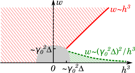
Figure 2: (Color online) Different regimes for the problem (5) with $E_{\mathrm{d}}(t)=h-wt^{2}$. The adibatic regime with $1-p_{\infty}\ll{1}$ (hatched area below the dashed line) occurs if the condition $|dE_{*}/dt|\ll{E}_{*}^{2}$ holds at all times. In the fast-drive regime (hatched area to the left of the solid line), the time spent in the continuum is too short, so that $h$ is within the energy uncertainty and $1-p_{\infty}\ll{1}$. In the Golden-Rule regime (white area between the dashed and the solid line) $p_{\infty}\ll{1}$. The grey area corresponds to $h^{3}\sim{w}\sim\gamma_{0}^{2}\Delta$ with $p_{\infty}\sim{1}$.

The adiabatic effect is nontrivial when the bound state is shallow, $h\gg(\gamma_{0}^{2}\Delta)^{1/3}$. We also assume $h^{3}\gg{w}$; otherwise, the time spent by $E_{\mathrm{d}}(t)$ in the continuum is too short (the energy uncertainty exceeds $h$), and $p_{\infty}\approx{1}$ can be found from Eq. (7) with $F(E)=2\pi{w}^{-1/3}\mathop{\mathrm{Ai}}\nolimits({w}^{-1/3}(E-h))$, where $\mathop{\mathrm{Ai}}\nolimits(x)$ is the Airy function. When $h^{3}\gg{w},\gamma_{0}^{2}\Delta$ (below the red solid line in Fig. 2), the wave function $\tilde{\psi}(E)$ can be found in the WKB approximation everywhere except (i) the vicinity of the classical turning point $E=h$, where it can be treated in the standard way, and (ii) near the singularity at $E\to{0}$ (see Supplemental Material for details). Then, one can identify two limiting cases for matching the WKB solution at $E\to{0}$, governed by the parameter $\sqrt{wh^{3}}/(\gamma_{0}^{2}\Delta)$. They are separated by the dashed line in Fig. 2.

(i) In the adiabatic regime, $\sqrt{wh^{3}}\gg\gamma_{0}^{2}\Delta$, the particle stays in the ground state up to an exponentially small ejection probability,

$$p_{\infty}=1-\exp\left(-\frac{\pi}{4}\,\frac{\gamma_{0}^{2}\Delta}{\sqrt{wh^{3}}}\right).$$ (13)

(ii) In the opposite limit, $C_{+}/C_{-}$ is calculated to the first order in $\sqrt{wh^{3}}/(\gamma_{0}^{2}\Delta)\ll{1}$, which gives

$$p_{\infty}=\left|e^{-\pi\sqrt{\gamma_{0}^{2}\Delta/(2w)}-(4/3)i\sqrt{h^{3}/w}}+e^{i\pi/4}\sqrt{\frac{\pi}{4}\,\frac{\gamma_{0}^{2}\Delta}{\sqrt{wh^{3}}}}\right|^{2}.$$ (14)

The first term [of zero order in $\sqrt{wh^{3}}/(\gamma_{0}^{2}\Delta)$] gives the Golden-Rule expression (1); indeed, the exponent is nothing but $(1/2)\int\Gamma(E_{\mathrm{d}}(t))\,dt-i\int{E}_{\mathrm{d}}(t)\,dt$ for $E_{\mathrm{d}}(t)=h-wt^{2}$. The second term is the first-order correction which must be small compared to unity, but can still be larger than the zero-order term. Remarkably, in the latter case it matches the adiabatic expression (13) obtained in the opposite limit.

Discussion. Equations (7), (13) and (14) represent the main result of the present work. They agree with the numerical solution of Eq. (5) (see the Supplemental Material). Although Eqs. (13) and (14) are obtained for a specific dependence $E_{\mathrm{d}}(t)=h-wt^{2}$, their relevance is quite general, since any smooth $E_{\mathrm{d}}(t)$ can be approximated by a parabola near the maximum. The three expressions have overlapping domains of validity: Eq. (7) with $F(E)=2\pi{w}^{-1/3}\mathop{\mathrm{Ai}}\nolimits({w}^{-1/3}(E-h))$ matches the first term in Eq. (14), while Eq. (13) matches the second. The only region not covered by Eqs. (7), (13) and (14) is $h^{3}\sim{w}\sim\gamma_{0}^{2}\Delta$, shown in Fig. 2 by the grey area.

Eq. (14) has a two-path form, corresponding to the two trajectories shown in Fig. 1. Due to the $h$- and $w$-dependent phase of the first term, $p_{\infty}$ may exhibit Stueckelberg interference oscillations as a function of $h$ or $w$. From the analogy with the standard two-level problem, it is tempting to assume that the crossing of the singularity at $t_{0}=-\sqrt{h/w}$ can be viewed as a beam splitter, when the particle “decides” which path to follow. However, if this were the case, the system behavior would be determined by $E_{\mathrm{d}}(t)$ linearized around $t_{0}$, i. e., by $\dot{E}_{\mathrm{d}}(t_{0})=2\sqrt{wh}$, while in Eq. (14) the parameter governing the amplitude of the adiabatic path is $\sqrt{wh^{3}}/(\gamma_{0}^{2}\Delta)$. This latter parameter is nothing but the maximal value of $E_{*}^{-2}|dE_{*}/dt|$, which should be small to keep the adiabaticity at all times. This maximal value is reached at $t\approx t_{0}/\sqrt{3}$, quite far from the crossing.

In any realistic superconduncting device, the BCS singularity in the DOS, which is the key ingredient of the problem, is necessarily smeared on some energy scale. If the smearing exceeds $|E_{*}|$, the bound state enters the continuum and decays, so the described effect is no longer relevant. The smearing is often quantified by the Dynes parameter Dynes et al. (1978, 1984) which gives the ratio of the smearing scale to the gap $\Delta$. For aluminum-based superconducting nanostructures, the Dynes parameter is typically $10^{-4}-10^{-5}$, mostly due to microwave noise from the environment Pekola et al. (2010), and can be made as low as $10^{-7}$ if special efforts are made to ensure efficient microwave shielding and quasiparticle relaxation Saira et al. (2012). Taking the values $\gamma_{0}=1\>\mu\mbox{eV}$, $\Delta=200\>\mu\mbox{eV}$ van Zanten et al. (2015), we obtain the main energy scale responsible for the formation of the bound state $(\gamma_{0}^{2}\Delta/2)^{1/3}\approx{5}\>\mu\mbox{eV}$, which exceeds the Dynes smearing by several orders of magnitude. For a sinusoidal drive with the amplitude $100\>\mu\mbox{eV}$ and frequency $50\>\mbox{MHz}$ van Zanten et al. (2016), we obtain $w\approx{2}\>\mu\mbox{eV}^{3}$. Then the level should be pushed by $h\sim[(\gamma_{0}^{2}\Delta/2)^{2}/w]^{1/3}\sim$ a few $\mu$eV beyond the BCS singularity to overcome the adiabatic blocking, and the period of the Stueckelberg oscillations is $h\sim{w}^{1/3}\sim{1}\>\mu\mbox{eV}$, both corresponding to quite measurable energy scales. To give a noticeable amplitude of the oscillations, $w$ should not be too small compared to $\pi^{2}\gamma_{0}^{2}\Delta/2$, so it is better to use a device with sub-$\mu\mbox{eV}$ $\gamma_{0}$.

The experimental resolution is more likely to be limited by the high-frequency noise component of the driven gate voltage, which should favor electron ejection from the bound state into the continuum. Thus, in experiment, special care should be taken in order to reduce this extrinsic noise. Theoretically, the effect of noise has been studied for the standard two-level Landau-Zener problem Shimshoni and Gefen (1991); Shytov et al. (2003); Pokrovsky and Sinitsyn (2003); Vestgården et al. (2008); Whitney et al. (2011); Kenmoe et al. (2013); inclusion of noise in the present theory along the same lines is a subject for the future work.

To conclude, I presented an extension of the Landau-Zener problem to a continuous energy spectrum. The key role is played by the singularity in the continuum DOS, which is crossed by the driven discrete level. The Landau-Zener physics is not washed out by the continuum because of the quantum-mechanical level repulsion between the discrete level and the DOS singularity, and even Stueckelberg oscillations are present. The fundamental physics, described here, is shown to be relevant for a specific mesoscopic device, the hybrid quantum electron turnstile, where the BCS singularity in the quasiparticle DOS of superconducting electrodes may prevent electron ejection from the discrete quantum dot level into the electrode, thereby providing a fundamental limit on the device operation.

Supplemental Material

Analytical solution of the stationary Schrödinger equation

Here we study the stationary Schrödinger equation,

$$-w\,\frac{d^{2}\tilde{\psi}(E)}{dE^{2}}+V(E)\,\tilde{\psi}(E)=h\tilde{\psi}(E),$$ (15)

where $E$ plays the role of the coordinate, $1/(2w)$ and $h$ represent the mass and the energy, respectively, and

$$V(E)=E+\sqrt{\frac{\gamma_{0}^{2}\Delta}{-2E}}$$ (16)

is the effective potential, plotted in Fig. 3. $V(E)$ is real at $E<0$, while at $E>0$ the square root should be analytically continued in the upper complex half-plane, giving $\mathop{\mathrm{Im}}\nolimits{V}(E)>0$. The probability current, defined as

$$J(E)=-iw\left[\tilde{\psi}^{*}(E)\,\frac{d\tilde{\psi}(E)}{dE}-\frac{d\tilde{\psi}^{*}(E)}{dE}\,\tilde{\psi}(E)\right],$$ (17)

satisfies the continuity equation,

$$\frac{dJ(E)}{dE}=2\mathop{\mathrm{Im}}\nolimits{V}(E)\,|\tilde{\psi}(E)|^{2}.$$ (18)

Since $\tilde{\psi}(E\to+\infty)$ must be exponentially decaying, Eq. (18) implies $J(E)<0$, which ensures $p_{\infty}<1$.

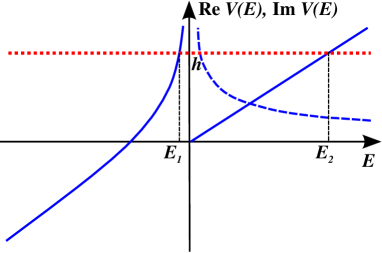
Figure 3: (Color online) The real and imaginary parts of the potential $V(E)$ (the blue solid and dashed curves, respectively). The energy $h$ is shown by the horizontal red dotted line. The scattering problem corresponds to the wave incident from the left, tunnelling under the square-root spike, and propagating until $E=E_{2}$, where it is necessarily reflected. While propagating at $E>0$, the wave is amplified due to $\mathop{\mathrm{Im}}\nolimits{V}(E)>0$.

In the following, we assume $h^{3}\gg{w},\gamma_{0}^{2}\Delta$. Then on most of the real axis, the solution can be approximated by the WKB form:

$$\tilde{\psi}(E\to-\infty)=\left(\frac{h}{w}\right)^{1/4}\sum_{\pm}C_{\pm}\frac{e^{\pm{i}S(E)}}{\sqrt{S^{\prime}(E)}},$$ (19)

$$S(E)=\int_{E_{1}}^{E}\sqrt{\frac{h-V(\varepsilon)}{w}}\,d\varepsilon,$$ (20)

where $S^{\prime}(E)\equiv{dS}/dE$, and we choose the lower limit $E_{1}$ to be the leftmost classical turning point of $V(E)$, where $V(E)=h$. Potential (16) has two turning points:

$$E_{1}=-\frac{\gamma_{0}^{2}\Delta}{2h^{2}}+O((\gamma_{0}^{2}\Delta)/h^{5}),\quad E_{2}=h+O\!\left(\sqrt{\gamma_{0}^{2}\Delta/h}\right)$$ (21)

(note that $E_{2}$ is complex). The conditions $h^{3}\gg{w},\gamma_{0}^{2}\Delta$ ensure that $E_{1}$ and $E_{2}$ are well separated, so that one can use the WKB expression in the region $0<E<E_{2}$. In fact, $E_{1}$ and $E_{2}$ are nothing but the poles of the Green’s function $G_{\mathrm{d}}(E)$ from Eq. (4) for $E_{\mathrm{d}}=h$, so the considered regime correponds to well separated peaks in the discrete level spectral function.

Let us introduce two pairs of WKB solutions, $\xi_{\pm}(E)$ and $\eta_{\pm}(E)$, representing the right/left-traveling waves in the regions $E<E_{1}$ and $0<E<E_{2}$, respectively:

$$\xi_{\pm}(E<E_{1})=\left(\frac{h}{w}\right)^{1/4}\frac{e^{\pm{i}S(E)}}{\sqrt{S^{\prime}(E)}},$$ (22)

$$\eta_{\pm}(0<E<E_{2})=\left(\frac{h}{w}\right)^{1/4}\frac{e^{\pm{i}S(E)}}{\sqrt{S^{\prime}(E)}}.$$ (23)

While $S(E<E_{1})$ is defined by the integral in Eq. (20) on the real axis, $S(0<E<E_{2})$ should be understood as the analytical continuation from $E<E_{1}$ through the upper complex half-plane. The two pairs of solutions must be linear combinations of each other, so we can define a transfer matrix $\mathcal{T}_{\kappa\kappa^{\prime}}$ with $\kappa,\kappa^{\prime}=\pm$, such that

$$\eta_{\kappa}(E)=\sum_{\kappa^{\prime}=\pm}\mathcal{T}_{\kappa\kappa^{\prime}}\xi_{\kappa^{\prime}}(E).$$ (24)

The Wronskian conservation, $W(\xi_{+},\xi_{-})=W(\eta_{+},\eta_{-})=-2i\sqrt{h/w}$, imposes $\det\mathcal{T}=1$.

At the turning point $E=E_{2}$ (even for complex $E_{2}$), $V(E)$ can be linearized, so the solution decaying at $E\to+\infty$ is constructed by the standard WKB prescription:

$$\tilde{\psi}(E)=\frac{2(h/w)^{1/4}}{\sqrt{S^{\prime}(E)}}\cos\left[S(E)-S(E_{2})+\frac{\pi}{4}\right]=$$

$$\qquad{}=\sum_{\kappa=\pm}e^{i\kappa[\pi/4-S(E_{2})]}\eta_{\kappa}(E)=$$

$$\qquad{}=\sum_{\kappa,\kappa^{\prime}=\pm}e^{i\kappa[\pi/4-S(E_{2})]}\mathcal{T}_{\kappa\kappa^{\prime}}\xi_{\kappa^{\prime}}(E).$$ (25)

As discussed in the main text, $p_{\infty}$ is determined by the ratio of the coefficients at $\xi_{+}(E)$ and $\xi_{-}(E)$:

$$p_{\infty}=\left|\frac{\mathcal{T}_{-+}+i\mathcal{T}_{++}e^{-2iS(E_{2})}}{\mathcal{T}_{--}+i\mathcal{T}_{+-}e^{-2iS(E_{2})}}\right|^{2}.$$ (26)

This reduces the problem to (i) evaluating $S(E_{2})$ and (ii) finding the matrix $\mathcal{T}_{\kappa\kappa^{\prime}}$, determined by the scattering on the singularity of the potential $V(E)$.

To find $S(E_{2})$, let us expand

$$S^{\prime}(E)=\sqrt{\frac{h-E}{w}-\sqrt{\frac{\gamma_{0}^{2}\Delta}{-2w^{2}E}}}$$ (27)

in $\sqrt{\gamma_{0}^{2}\Delta}$, and integrate it term by term:

$$S(E)=\frac{2}{3}\sqrt{\frac{h^{3}}{w}}-\frac{2}{3}\sqrt{\frac{(h-E)^{3}}{w}}+{}$$

$$\quad\qquad{}+\sqrt{\frac{\gamma_{0}^{2}\Delta}{2w}}\mathop{\mathrm{arcsinh}}\nolimits\sqrt{-\frac{E}{h}}+{}$$

$$\quad\qquad{}+O\!\left(\sqrt{\frac{\gamma_{0}^{2}\Delta}{w}}\sqrt{\frac{\gamma_{0}^{2}\Delta}{(h-E)^{3}}}\,\ln(-E)\right).$$ (28)

This expression describes $S(E)$ at $E<E_{1}$, while for $E>0$ the analytical continuation gives $\sqrt{-E}\to-i\sqrt{E}$, $\mathop{\mathrm{arcsinh}}\nolimits\sqrt{-E/h}\to-i\arcsin\sqrt{E/h}$. This imaginary term in $S(E)$ produces the enhancement of the propagating waves in the region $0<E<h$, required by Eq. (18). Expansion (28) breaks down at $E\to{h}$. Let us now expand around $E=E_{2}$:

$$S(E)=S(E_{2})-\frac{2}{3}\left(1-\frac{i}{4}\sqrt{\frac{\gamma_{0}^{2}\Delta}{2h^{3}}}\right)\sqrt{\frac{(E_{2}-E)^{3}}{w}}+{}$$

$$\quad\qquad{}+O\!\left(\sqrt{\frac{\gamma_{0}^{2}\Delta}{w}}\sqrt{\frac{(E_{2}-E)^{5}}{h^{5}}}\right).$$ (29)

Expansion (28) assumes $h-E\gg\sqrt{\gamma_{0}^{2}\Delta/h}$, while expansion (29) assumes $|E_{2}-E|\ll{h}$, so they can be matched in the parametrically wide region where both inequalities are satisfied. This gives the leading real and imaginary terms in $S(E_{2})$:

$$S(E_{2})\approx\frac{2}{3}\sqrt{\frac{h^{3}}{w}}-\frac{i\pi}{2}\sqrt{\frac{\gamma_{0}^{2}\Delta}{2w}}.$$ (30)

Note that subleading terms $\sim\gamma_{0}^{2}\Delta/\sqrt{wh^{3}}$ can still be larger than unity. It will be seen below that the precise value of $S(E_{2})$ is not important for $wh^{3}\ll(\gamma_{0}^{2}\Delta)^{2}$.

To determine the matrix $\mathcal{T}_{\kappa\kappa^{\prime}}$, one can neglect the linear term $E$ in the potential $V(E)$ because $|E_{1}|\ll{h}$. Then, it is convenient to rescale the energy, $E=y\sqrt{w/h}$, and rewrite the Schrödinger equation as

$$-\frac{d^{2}\tilde{\psi}}{dy^{2}}+\frac{\alpha}{\sqrt{-y}}\,\tilde{\psi}=\tilde{\psi},\quad\alpha\equiv\sqrt{\frac{\gamma_{0}^{2}\Delta/2}{\sqrt{wh^{3}}}}.$$ (31)

This equation has an exact solution, expressed in terms of the confluent hypergeometric function Ishkhanyan (2015). Still, the two limiting cases $\alpha\ll{1}$ and $\alpha\gg{1}$ can be analyzed without invoking the exact solution. This is done below, and simple expressions for $p_{\infty}$ are obtained.

For $\alpha=0$ one trivially obtains $\mathcal{T}_{\kappa\kappa^{\prime}}=\delta_{\kappa\kappa^{\prime}}$. When substituted in Eq. (26), it gives the first term in Eq. (14), that is, the Golden-Rule result (1).

For $\alpha\ll{1}$ one can calculate the first perturbative correction to $\mathcal{T}_{\kappa\kappa^{\prime}}=\delta_{\kappa\kappa^{\prime}}$. Let us look for two linearly independent solutions of Eq. (31) in the form $\tilde{\psi}(y)=[1+\alpha{u}(y)]e^{\pm{iy}}$. Then $u(y)$ satisfies $u^{\prime\prime}\pm{2}iu^{\prime}=1/\sqrt{-y}$, and writing further $u^{\prime}(y)=v(y)\,e^{\mp{2}iy}$, we obtain the wave functions in the form

$$\tilde{\psi}(y)=e^{\pm{i}y}+\alpha{}e^{\pm{i}y}\int\limits^{y}dy_{1}\int\limits^{y_{1}}dy_{2}\,\frac{e^{\pm{2}i(y_{2}-y_{1})}}{\sqrt{-y_{2}}}+O(\alpha^{2}).$$ (32)

Taking different lower integration limits corresponds to forming different linear combinations of $\xi_{\pm}(y)$ or $\eta_{\pm}(y)$, and one is free to choose the most convenient one. Indeed, to find the matrix $\mathcal{T}_{\kappa\kappa^{\prime}}$ it is sufficient to construct any pair of linearly independent solutions and to match it to $\xi_{\pm}$ and $\eta_{\pm}$. Choosing both lower limits to be zero and integrating over $y_{1}$ by parts, one readily obtains a compact expression in terms of the error function:

$$\tilde{\psi}(y)=e^{\pm{i}y}\pm{i}\alpha\sqrt{-y}\,{}e^{\pm{i}y}+{}$$

$$\qquad\quad{}+\alpha\sqrt{\frac{\pi}{8}}\,e^{\mp{3}i\pi/4\mp{i}y}\mathop{\mathrm{erf}}\nolimits\!\left(\sqrt{-2y}\,e^{\pm{i}\pi/4}\right)+O(\alpha^{2}).$$

(33)

Let us now write the expansion of the WKB solutions $(1-\alpha/\sqrt{-y})^{-1/4}e^{\pm{i}S(y)}$ with $S(y)=y+\alpha\sqrt{-y}$ (28):

$$\xi_{\pm}(y<0)=\left(1+\frac{1}{4}\,\frac{\alpha}{\sqrt{-y}}\pm{i}\alpha\sqrt{-y}\right)e^{\pm{i}y}+O(\alpha^{2}),$$

(34)

$$\eta_{\pm}(y>0)=\left(1+\frac{i}{4}\,\frac{\alpha}{\sqrt{y}}\pm\alpha\sqrt{y}\right)e^{\pm{i}y}+O(\alpha^{2}).$$ (35)

To match them to Eq. (33), one should use the asymptotic expression for $\mathop{\mathrm{erf}}\nolimits(z)$ paying attention to the essential singularity at $z=\infty$, so that for real $s\to+\infty$

$$\mathop{\mathrm{erf}}\nolimits(se^{\pm{i}\pi/4})=1-\frac{e^{\mp{is^{2}}\mp{i}\pi/4}}{\sqrt{\pi}{s}}+O(1/s^{2}),$$

but at the same time, due to $\mathop{\mathrm{erf}}\nolimits(-z)=-\mathop{\mathrm{erf}}\nolimits(z)$,

$$\mathop{\mathrm{erf}}\nolimits(se^{-3i\pi/4})=-1+\frac{e^{-is^{2}-i\pi/4}}{\sqrt{\pi}{s}}+O(1/s^{2}).$$

The result is

$$\tilde{\psi}(y)=\xi_{\pm}(y)+\alpha\sqrt{\frac{\pi}{8}}\,e^{\mp{3}i\pi/4}\xi_{\mp}(y)+O(\alpha^{2})=$$

$$\qquad{}=\eta_{\pm}(y)\pm\alpha\sqrt{\frac{\pi}{8}}\,e^{\mp{3}i\pi/4}\eta_{\mp}(y)+O(\alpha^{2}),$$ (36)

from which $\mathcal{T}_{\kappa\kappa^{\prime}}$ is obtained to the first order in $\alpha$:

$$\mathcal{T}_{++},\mathcal{T}_{--}=1+O(\alpha^{2}),\quad\mathcal{T}_{+-}=O(\alpha^{2}),$$ (37)

$$\mathcal{T}_{-+}=\alpha\sqrt{\frac{\pi}{2}}\,e^{3i\pi/4}+O(\alpha^{2}).$$ (38)

Its substitution into (26) gives the second term in (14).

For $\alpha\gg{1}$, the key observation is that the classical turning point $y=-\alpha^{2}$ lies quite far from the singularity at $y=0$, so there is a wide classically forbidden region between $-\alpha^{2}$ and 0. As a result, only an exponentially small part of the incident wave will be able to tunnel to the amplification zone at $y>0$. Moreover, in most of the classically forbidden region the WKB approximation can be used, so up to exponentially small terms the sought solution $\tilde{\psi}(y)$ can be written in the standard WKB form:

$$\tilde{\psi}(y<-\alpha^{2})=e^{i\pi/4}\xi_{+}(y)+e^{-i\pi/4}\xi_{-}(y),$$ (39)

$$\tilde{\psi}(-\alpha^{2}<y<0)=\frac{e^{-\sigma(y)}}{\sqrt{\sigma^{\prime}(y)}},$$ (40)

where $\sigma^{\prime}(y)=d\sigma(y)/dy$ and $\sigma(y)$ is just $\mathop{\mathrm{Im}}\nolimits{S}$ in the forbidden region:

$$\sigma(y)=\int\limits_{-\alpha^{2}}^{y}\sqrt{\frac{\alpha}{\sqrt{-y_{1}}}-1}\,dy_{1}={}$$

$$\qquad{}=\frac{\alpha^{2}}{4}\arccos\left(\frac{2\sqrt{-y}}{\alpha}-1\right)-{}$$

$$\qquad\quad{}-\left(\sqrt{-y}-\frac{\alpha}{2}\right)\sqrt{\alpha\sqrt{-y}+y}.$$ (41)

Keeping the exponentially growing solution $\propto{e}^{\sigma(y)}$ in the whole region $-a^{2}<y<0$ is beyond the WKB accuracy. However, one should keep in mind that at $y\to{0}$ its amplitude is of the same order as that of solution (40). At $|y|\sim\alpha^{-2/3}$, the WKB approximation breaks down; however, at $|y|\ll\alpha^{2}$ one can neglect the right-hand side of Eq. (31) and solve it exactly, obtaining two linearly independent solutions. At positive $y\gg\alpha^{-2/3}$, the WKB approximation is again valid, and the sought solution $\tilde{\psi}(y)$ is a linear combination of $\eta_{\pm}(y)$, with the amplitude of $\eta_{+}(y)$ being exponentially smaller than that of $\eta_{-}(y)$, according to Eq. (25). Thus, one can neglect the $\eta_{+}$ component and solve Eq. (31) with zero right-hand side and with the boundary condition of exponentially decaying $\tilde{\psi}(y)\propto\eta_{-}(y)$ at $y\to+\infty$. At $y\to-\infty$ the solution will have both $e^{\sigma(y)}$ and $e^{-\sigma(y)}$ components, and the amplitude of the latter is given by Eq. (40).

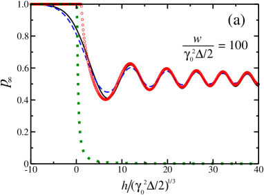
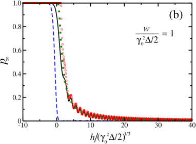
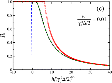
Figure 4: (Color online) Comparison between the different analytical expressions for $p_{\infty}$ from the main text and the results of the numerical integration for $w/(\gamma_{0}^{2}\Delta/2)=100,\,1,\,0.01$, shown on panels (a), (b), (c), respectively. The black solid line represents the numerical result. The dashed blue line is the Markovian result, Eq. (7). The green squares represent the adiabatic result, Eq. (13). The red circles show the crossover expression, Eq. (14). The energies are measured in the units of $(\gamma_{0}^{2}\Delta/2)^{1/3}$.

When the right-hand side of Eq. (31) is neglected, by a substitution $y=-(4\alpha)^{-2/3}z^{2}$ it is reduced to the Airy equation, so the linearly independent solutions are the derivatives of the Airy functions:

$$\tilde{\psi}(y)=C_{\mathrm{A}}\mathop{\mathrm{Ai}}\nolimits^{\prime}\!\left((4\alpha)^{1/3}\sqrt{-y}\right)+C_{\mathrm{B}}\mathop{\mathrm{Bi}}\nolimits^{\prime}\!\left((4\alpha)^{1/3}\sqrt{-y}\right),$$ (42)

valid at $|y|\ll\alpha^{2}$. The coefficients $C_{\mathrm{A}},C_{\mathrm{B}}$ should be determined by matching the WKB solutions, as described above, at $\alpha^{2/3}\ll|y|\ll\alpha^{2}$. At $y<0$, expanding $\sigma(y)=\pi\alpha^{2}/4-(4/3)\sqrt{\alpha}(-y)^{3/4}+O((-y)^{5/4}$ and using the asymptotic expression $\mathop{\mathrm{Bi}}\nolimits^{\prime}(z)\approx{z}^{1/4}e^{-(2/3)z^{3/2}}/\sqrt{\pi}$ for real $z>0$, we obtain $C_{\mathrm{B}}=\sqrt{\pi}(2\alpha^{2})^{-1/6}e^{-\pi\alpha^{2}/4}$. At $y>0$, the exponentially decaying linear combination of $\mathop{\mathrm{Ai}}\nolimits^{\prime}(-is)$ and $\mathop{\mathrm{Bi}}\nolimits^{\prime}(-is)$ with real $s>0$ is obtained by taking $C_{\mathrm{A}}=iC_{\mathrm{B}}$.

Now, to find the exponentially small difference between $|C_{+}|$ and $|C_{-}|$ in Eq. (19) it is sufficient to evaluate the current. On the one hand, the current carried by solution (19) at $E<E_{1}$ is given by $J=2\sqrt{wh}(|C_{+}|^{2}-|C_{-}|^{2})$. On the other, from Eq. (18),

$$J=-2\sqrt{wh}\int\limits_{0}^{\infty}\frac{\alpha}{\sqrt{y}}\,|\tilde{\psi}(y)|^{2}\,dy.$$ (43)

For $\tilde{\psi}(y)$, it is sufficient to use expression (42) as the integral converges at $y\sim\alpha^{-2/3}\ll{1}$. This gives the leading exponential in $1-p_{\infty}$:

$$1-p_{\infty}\approx\pi{e}^{-\pi\alpha^{2}/2}\int\limits_{0}^{\infty}\left|i\mathop{\mathrm{Ai}}\nolimits^{\prime}(-is)+\mathop{\mathrm{Bi}}\nolimits^{\prime}(-is)\right|^{2}ds=$$

$$\hskip 42.67912pt{}={e}^{-\pi\alpha^{2}/2},$$ (44)

which is Eq. (13). The integral is calculated by parts:

$$\int\limits_{0}^{\infty}\left|i\mathop{\mathrm{Ai}}\nolimits^{\prime}(-is)+\mathop{\mathrm{Bi}}\nolimits^{\prime}(-is)\right|^{2}ds=$$

$$=\frac{1-i/\sqrt{3}}{\pi}+\int\limits_{0}^{\infty}\left|\mathop{\mathrm{Ai}}\nolimits(is)+i\mathop{\mathrm{Bi}}\nolimits(is)\right|^{2}is\,ds.$$ (45)

While the first line is purely real, the last integral is purely imaginary, so the first line must be equal to $1/\pi$.

Numerical solution of the dynamical problem

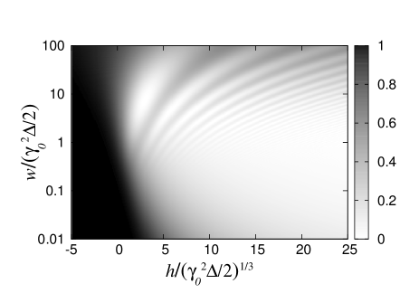
Figure 5: The numerical results for $p_{\infty}$ in the whole $(h,w)$ plane. The black and white color correspond to $p_{\infty}\to{1}$ and $p_{\infty}\to{0}$, respectively. The energies are measured in the units of $(\gamma_{0}^{2}\Delta/2)^{1/3}$.

To solve the dynamical problem numerically, it is more convenient to return to the original problem (2), (3), rather than to integrate Eq. (5) with the long-range memory kernel. Equations  (2) and  (3) can be equivalently rewritten in the coordinate representation, which is implemented numerically as a tight-binding model:

$$i\,\frac{\partial\psi_{\mathrm{d}}}{\partial{t}} = E_{\mathrm{d}}(t)\,\psi_{\mathrm{d}}+V\phi_{0},$$ (46)

$$i\,\frac{\partial\phi_{n}}{\partial{t}} = \delta_{n0}V\psi_{\mathrm{d}}+J(2\phi_{n}-\phi_{n-1}-\phi_{n+1}).$$ (47)

To determine the coefficients, it is convenient to consider the self-energy for the tight-binding model,

$$\Sigma^{\mathrm{TB}}(E)=\int\limits_{-\pi}^{\pi}\frac{V^{2}}{E-2J(1-\cos{k})}\,\frac{dk}{2\pi}=\frac{V^{2}\mathop{\mathrm{sign}}\nolimits(E-2J)}{\sqrt{E(E-4J)}},$$ (48)

and to match the coefficient at $1/\sqrt{E}$, which gives

$$\frac{V^{2}}{\sqrt{4J}}=\sqrt{\frac{\gamma_{0}^{2}\Delta}{2}}.$$ (49)

This still leaves a freedom of simultaneous rescaling of $V$ and $J$ which keeps $V^{2}/\sqrt{J}$ constant. The value of $J$ should be chosen so that the level energy is always in the parabolic part of the spectrum, $J\gg\max\{E_{\mathrm{d}},(\gamma_{0}^{2}\Delta)^{1/3}\}$.

It is convenient to impose periodic boundary conditions, $\phi_{n=N-1}=\phi_{n=-(N-1)}$, so that the chain has $2N-2$ sites, and to notice that the $(N-2)$-dimensional odd subspace $\phi_{n}=-\phi_{-n}$ decouples from the discrete level. Thus, one can work with the $N$-dimensional even subspace, for which the equations become

$$i\,\frac{\partial\phi_{0}}{\partial{t}}=V\psi_{\mathrm{d}}+2J(\phi_{0}-\phi_{1}),$$ (50)

$$i\,\frac{\partial\phi_{n}}{\partial{t}}=J(2\phi_{n}-\phi_{n-1}-\phi_{n+1}),\quad 0<n<N-1,\qquad$$ (51)

$$i\,\frac{\partial\phi_{N-1}}{\partial{t}}=2J(\phi_{N-1}-\phi_{N-2}).$$ (52)

The eigenstates of the unperturbed problem are

$$a_{kn}\propto\cos\frac{\pi{k}n}{N-1},\quad E_{k}=2J\left(1-\cos\frac{\pi{k}}{N-1}\right),$$ (53)

with $k=0,1,\ldots,N-1$. The length of the chain should be sufficiently large, so that

$$E_{k=1}-E_{k=0}\approx{J}\frac{\pi^{2}}{N^{2}}\ll|E_{*}|\approx\frac{\gamma_{0}^{2}\Delta}{2E_{\mathrm{d}}^{2}}.$$ (54)

The resulting system of ordinary differential equations is integrated using the Bulirsch-Stoer method with polynomial extrapolation. The results of the numerical integration for $E_{\mathrm{d}}(t)=h-wt^{2}$ are shown in Figs. 4 and 5, where $(\gamma_{0}^{2}\Delta/2)^{1/3}$ is used as the natural unit of energy. From Fig. 4 one can see that except the region $h^{3}\sim{w}\sim\gamma_{0}^{2}\Delta$, the numerical result is well captured by at least one of the three analytical expressions, Eqs. (7), (13), and (14). Remarkably, at $w\gg\gamma_{0}^{2}\Delta$, the Stueckelberg oscillations are reproduced both by the Markovian Eq. (7) and by the crossover Eq. (14).

References

- Landau (1932) L. D. Landau, “Zur Theorie der Energieubertragung. II,” Phys. Z. Sowjetunion 2, 46 (1932).
- Zener (1932) C. Zener, “Non-Adiabatic Crossing of Energy Levels,” Proc. R. Soc. A 137, 696 (1932).
- Stueckelberg (1932) E. C. G. Stueckelberg, “Theorie der unelastischen Stösse zwischen Atomen,” Helv. Phys. Acta 5, 369 (1932).
- Majorana (1932) E. Majorana, “Atomi orientati in campo magnetico variabile,” Nuovo Cimento 9, 43 (1932).
- May and Kuhn (2000) V. May and O. Kuhn, Charge and Energy Transfer Dynamics in Molecular Systems (Wiley–VCH-Verlag, 2000).
- Wernsdorfer and Sessoli (1999) W. Wernsdorfer and R. Sessoli, “Quantum Phase Interference and Parity Effects in Magnetic Molecular Clusters,” Science 284, 133 (1999).
- Sun et al. (2008) D. Sun, Ar. Abanov, and V. L. Pokrovsky, “Molecular production at a broad Feshbach resonance in a Fermi gas of cooled atoms,” EPL 83, 16003 (2008).
- Renzoni and Brandes (2001) F. Renzoni and T. Brandes, “Charge transport through quantum dots via time-varying tunnel coupling,” Phys. Rev. B 64, 245301 (2001).
- Kashcheyevs and Timoshenko (2012) V. Kashcheyevs and J. Timoshenko, “Quantum fluctuations and coherence in high-precision single-electron capture,” Phys. Rev. Lett. 109, 216801 (2012).
- Gefen and Thouless (1987) Y. Gefen and D. J. Thouless, “Zener transitions and energy dissipation in small driven systems,” Phys. Rev. Lett. 59, 1752 (1987).
- Schön and Zaikin (1990) G. Schön and A. D. Zaikin, “Quantum coherent effects, phase transitions, and the dissipative dynamics of ultra small tunnel junctions,” Phys. Rep 198, 237 (1990).
- Weißl et al. (2015) T. Weißl, G. Rastelli, I. Matei, I. M. Pop, O. Buisson, F. W. J. Hekking, and W. Guichard, “Bloch band dynamics of a Josephson junction in an inductive environment,” Phys. Rev. B 91, 014507 (2015).
- Demkov and Osherov (1968) Yu. N. Demkov and V. I. Osherov, “Stationary and nonstationary problems in quantum mechanics that can be solved by means of contour integration,” Sov. Phys. JETP 26, 916 (1968).
- Brundobler and Elser (1993) S. Brundobler and V. Elser, “S-matrix for generalized Landau-Zener problem,” J. Phys. A: Math. Gen. 26, 1211 (1993).
- Demkov et al. (1995) Yu. N. Demkov, P. B. Kurasov, and V. N. Ostrovsky, “Doubly periodical in time and energy exactly soluble system with two interacting systems of states,” J. Phys. A: Math. Gen. 28, 4361 (1995).
- Ostrovsky and Nakamura (1997) V. N. Ostrovsky and H. Nakamura, “Exact analytical solution of the -level Landau-Zener-type bow-tie model,” J. Phys. A: Math. Gen. 30, 6939 (1997).
- Demkov and Ostrovsky (2001) Yu. N. Demkov and V. N. Ostrovsky, “The exact solution of the multistate Landau-Zener type model: the generalized bow-tie model,” J. Phys. B: Atomic, Molecular and Optical Physics 34, 2419 (2001).
- Pokrovsky and Sinitsyn (2002) V. L. Pokrovsky and N. A. Sinitsyn, “Landau-Zener transitions in a linear chain,” Phys. Rev. B 65, 153105 (2002).
- Volkov and Ostrovsky (2004) M. V. Volkov and V. N. Ostrovsky, “Exact results for survival probability in the multistate Landau-Zener model,” J. Phys. B: Atomic, Molecular and Optical Physics 37, 4069 (2004).
- Shytov (2004) A. V. Shytov, “Landau-Zener transitions in a multilevel system: An exact result,” Phys. Rev. A 70, 052708 (2004).
- Patra and Yuzbashyan (2015) A. Patra and E. A. Yuzbashyan, “Quantum integrability in the multistate Landau-Zener problem,” J. Phys. A: Math. Theor. 48, 245303 (2015).
- Vitanov and Garraway (1996) N. V. Vitanov and B. M. Garraway, “Landau-Zener model: Effects of finite coupling duration,” Phys. Rev. A 53, 4288 (1996).
- Mkam Tchouobiap et al. (2015) S. E. Mkam Tchouobiap, M. B. Kenmoe, and L. C. Fai, “The finite time multi-level Landau–Zener problems: exact analytical results,” J. Phys. A: Math. Theor. 48, 395301 (2015).
- Keeling and Gurarie (2008) J. Keeling and V. Gurarie, “Collapse and Revivals of the Photon Field in a Landau-Zener process,” Phys. Rev. Lett. 101, 033001 (2008).
- Altland and Gurarie (2008) A. Altland and V. Gurarie, “Many Body Generalization of the Landau-Zener Problem,” Phys. Rev. Lett. 100, 063602 (2008).
- Ishkhanyan (2010) A. M. Ishkhanyan, “Generalized formula for the Landau-Zener transition in interacting Bose-Einstein condensates,” EPL 90, 30007 (2010).
- Demkov (1964) Yu. N. Demkov, “Detachment of electrons in slow collisions between negative ions and atoms,” Sov. Phys. JETP 19, 762 (1964).
- Pekola et al. (2013) J. P. Pekola, O.-P. Saira, V. F. Maisi, A. Kemppinen, M. Möttönen, Y. A. Pashkin, and D. V. Averin, “Single-electron current sources: Toward a refined definition of the ampere,” Rev. Mod. Phys. 85, 1421 (2013).
- Kaestner and Kashcheyevs (2015) B. Kaestner and V. Kashcheyevs, “Non-adiabatic quantized charge pumping with tunable-barrier quantum dots: a review of current progress,” Reports on Progress in Physics 78, 103901 (2015).
- Pekola et al. (2008) J. P. Pekola, J. J. Vartiainen, M. Mottonen, O.-P. Saira, M. Meschke, and D. V. Averin, “Hybrid single-electron transistor as a source of quantized electric current,” Nature Phys. 4, 120 (2008).
- van Zanten et al. (2015) D. M. T. van Zanten, F. Balestro, H. Courtois, and C. B. Winkelmann, “Probing hybridization of a single energy level coupled to superconducting leads,” Phys. Rev. B 92, 184501 (2015).
- van Zanten et al. (2016) D. M. T. van Zanten, D. M. Basko, I. M. Khaymovich, J. P. Pekola, H. Courtois, and C. B. Winkelmann, “Single Quantum Level Electron Turnstile,” Phys. Rev. Lett. 116, 166801 (2016).
- Fetter (1965) A. L. Fetter, “Spherical impurity in an infinite superconductor,” Phys. Rev. 140, A1921–A1936 (1965).
- Machida and Shibata (1972) K. Machida and F. Shibata, “Bound States Due to Resonance Scattering in Superconductor,” Prog. Theor. Phys. 47, 1817 (1972).
- Shiba (1973) H. Shiba, “A Hartree-Fock Theory of Transition-Metal Impurities in a Superconductor,” Prog. Theor. Phys. 50, 50 (1973).
- Yu (1965) L. Yu, “Bound state in superconductors with paramgnetic impurities,” Acta Physica Sinica 21, 75 (1965).
- Soda et al. (1967) T. Soda, T. Matsuura, and Y. Nagaoka, “- Exchange Interaction in a Superconductor,” Progress of Theoretical Physics 38, 551 (1967).
- Shiba (1968) H. Shiba, “Classical Spins in Superconductors,” Progress of Theoretical Physics 40, 435 (1968).
- Rusinov (1969) A. I. Rusinov, “Superconductivity near a paramgnetic impurity,” JETP Lett. 9, 85 (1969).
- Note (1) The author has not succeeded in obtaining any result working in the time-dependent adiabatic basis.
- Dynes et al. (1978) R. C. Dynes, V. Narayanamurti, and J. P. Garno, “Direct measurement of quasiparticle-lifetime broadening in a strong-coupled superconductor,” Phys. Rev. Lett. 41, 1509–1512 (1978).
- Dynes et al. (1984) R. C. Dynes, J. P. Garno, G. B. Hertel, and T. P. Orlando, “Tunneling study of superconductivity near the metal-insulator transition,” Phys. Rev. Lett. 53, 2437–2440 (1984).
- Pekola et al. (2010) J. P. Pekola, V. F. Maisi, S. Kafanov, N. Chekurov, A. Kemppinen, Yu. A. Pashkin, O.-P. Saira, M. Möttönen, and J. S. Tsai, “Environment-assisted tunneling as an origin of the dynes density of states,” Phys. Rev. Lett. 105, 026803 (2010).
- Saira et al. (2012) O.-P. Saira, A. Kemppinen, V. F. Maisi, and J. P. Pekola, “Vanishing quasiparticle density in a hybrid Al/Cu/Al single-electron transistor,” Phys. Rev. B 85, 012504 (2012).
- Shimshoni and Gefen (1991) E. Shimshoni and Y. Gefen, “Onset of Dissipation in Zener Dynamics: Relaxation versus Dephasing,” Ann. Phys. (N. Y.) 210, 1680 (1991).
- Shytov et al. (2003) A. V. Shytov, D. A. Ivanov, and M. V. Feigel’man, “Landau-Zener interferometry for qubits,” Eur. Phys. J. B 36, 263 (2003).
- Pokrovsky and Sinitsyn (2003) V. L. Pokrovsky and N. A. Sinitsyn, “Fast noise in the Landau-Zener theory,” Phys. Rev. B 67, 144303 (2003).
- Vestgården et al. (2008) J. I. Vestgården, J. Bergli, and Y. M. Galperin, “Nonlinearly driven Landau-Zener transition in a qubit with telegraph noise,” Phys. Rev. B 77, 014514 (2008).
- Whitney et al. (2011) R. S. Whitney, M. Clusel, and T. Ziman, “Temperature Can Enhance Coherent Oscillations at a Landau-Zener Transition,” Phys. Rev. Lett. 107, 210402 (2011).
- Kenmoe et al. (2013) M. B. Kenmoe, H. N. Phien, M. N. Kiselev, and L. C. Fai, “Effects of colored noise on Landau-Zener transitions: Two- and three-level systems,” Phys. Rev. B 87, 224301 (2013).
- Ishkhanyan (2015) A. M. Ishkhanyan, “Exact solution of the Schrödinger equation for the inverse square root potential ,” EPL 112, 10006 (2015).