A Perron–Frobenius type result for integer maps
and applications

Abstract.

It is shown that for certain maps, including concave maps, on the $d$-dimensional lattice of positive integer points, ‘approximate’ eigenvectors can be found. Applications in epidemiology as well as distributed resource allocation are discussed as examples.

1. Introduction

The classical linear Perron–Frobenius theorem goes back to the work of Oskar Perron, who studied the eigenvalue problem $Ax=\lambda x$ for positive matrices, and later Georg Frobenius, who extended the result to non-negative irreducible matrices. The theorem asserts the existence of a positive eigenvalue equal to the spectral radius and a corresponding positive, respectively, non-negative eigenvector. This theorem has found various applications in economics, the study of Markov chains, differential equations, and more. A detailed discussion of this and related results can be found, e.g., in the books [BP94, Gan59].

It is also possible to study eigenvectors in a nonlinear setting. Nonlinear Perron–Frobenius results appeared already in [SS53]. Later, a new approach to the eigenvalue problem was introduced in the work of Birkhoff [Bir57] and Samelson [Sam57]. This new approach enabled the study of eigenvalues and eigenvectors for a large class of nonlinear positive maps. There is now a rich literature on Perron–Frobenius results for nonlinear positive maps. One area in which Perron–Frobenius theory has been found useful is the area of economic theory, for example in questions related to price stability, cf., e.g., [Koh82]*Sec. 2. Indeed, many of the Perron–Frobenius results, such as [Koh82, Kra86, MF74, SS53] appeared in economics journals, cf., [Mor64, Nik68].

Convex and concave maps appear often in economics, cf., e.g., [Nik68], so quite a few Perron–Frobenius type results have been studied for this case, e.g., by [Kra86]. The notion of concavity can also be studied in a discrete setting, cf. [BG18]. Other Perron–Frobenius type results can be found in [Ch14, KP82, Kra01, Nus88] to mention just a few. Finally, the book [LN12] gives a good introduction to the nonlinear Perron–Frobenius theory.

The approach introduced in [Bir57, Sam57] can be described in the following way. Suppose that $A$ is a positive map in a $d$-dimensional space, that is $A:\mathbb{R}_{+}^{d}\to\mathbb{R}_{+}^{d}$, where here and in what follows $\mathbb{R}_{+}=[0,\infty)$ denotes all non-negative real numbers. The key idea is to consider the normalized map $Bx=Ax/\|Ax\|$, where $\|\cdot\|$ is some norm on $\mathbb{R}^{d}$, and then to show that with respect to a given metric (typically the Hilbert projective metric, see Section 2 for the precise definition), the map $B$ is well behaved and leaves invariant some compact subset of $\mathbb{R}_{+}^{d}$. Then, using a fixed point result such as the Banach contraction principle or the Brouwer fixed point theorem, it follows that there exists a vector $x\in\mathbb{R}_{+}^{d}$ such that $Bx=x$. This fixed point is the desired eigenvector, as we have $Ax=\|Ax\|\,x$.

In this paper we consider maps $A:\mathbb{Z}_{+}^{d}\to\mathbb{Z}_{+}^{d}$, where here and in what follows $\mathbb{Z}_{+}=\{0,1,\dots\}$ denotes all non-negative integers, while $\mathbb{N}=\{1,2,\dots\}$. Where previous results focus on maps defined on $\mathbb{R}_{+}^{d}$ (and in some cases on infinite dimensional Banach spaces), here we show that with reasonable adaptation of the existing tools it is possible to study maps in a discrete setting. As many of the classical applications of Perron–Frobenius theory are in fact continuous approximations of discrete models, the use of a discrete Perron–Frobenius theory gives a different, more direct, approach to dealing with such problems.

To this end, in order to use fixed point theorems, we show that under certain conditions the map $A$ can be extended to a well behaved map on a compact, convex set in $\mathbb{R}_{+}^{d}$. Since the fixed point of the extended map $B$ may be a non-integer point, we only have an ‘approximate’ eigenvector, which is suitably characterized by inequalities. A notion of concavity, originally introduced for groups in [BG18], is used to study discrete, concave maps.

This paper is organized as follows. The main result is given in Section 2. Theorem 2.2 extends the classic Perron–Frobenius theorem to discrete maps on the $d$-dimensional positive integer lattice. Corollary 2.1 shows that under the assumption that the norm of $Ax$ is well behaved, we may obtain a sequence in $\mathbb{Z}_{+}^{d}$ with controlled growth or decay. In Section 3 we show that the main result can be applied to concave maps on $\mathbb{Z}_{+}^{d}$. In Section 4, it is shown how the results of Section 2 and Section 3 can be applied to models from biology and engineering. In particular, we study a discrete variant of the Susceptible-Infected-Susceptible (SIS) model, as well as two models from communications: the Additive Increase Multiplicative Decrease (AIMD) model and an interference constraints model for wireless communication systems.

Acknowledgements

This paper was written while both authors were members of the priority research centre for Computer-Assisted Research Mathematics and its Applications (CARMA) at the University of Newcastle, Australia (UON). CARMA was founded in 2009 by Jonathan M. Borwein, who also served as its director. Jon was a prolific researcher and a devoted friend. This paper is dedicated to his memory with admiration.

2. Approximate eigenvectors for integer maps

Before we can state and prove the main result, we recall some basic notations that will be used throughout this paper. Let $\mathbb{R}_{+}^{d}$ denote the non-negative orthant in $\mathbb{R}^{d}$, which is a cone. Given two vectors $x=(x_{1},\dots,x_{d})$ and $y=(x_{1},\dots,x_{d})$ in $\mathbb{R}_{+}^{d}$, let $\leq$ denote the standard (component-wise) partial order induced by this cone, that is,

$$x \leq y \iff y-x \in\mathbb{R}_{+}^{d} \iff \big{[}x_{i}\leq y_{i}~{}\forall i\in\{1,\dots,d\}\big{]},$$

and also denote

$$x \ll y \iff y-x \in(0,\infty)^{d} \iff \big{[}x_{i}<y_{i}~{}\forall i\in\{1,\dots,d\}\big{]}.$$

Note that the maximum and minimum with respect to the cone partial order coincide with component-wise maximum and minimum.

Given $x,y\in\mathbb{R}^{d}_{+}\setminus\{0\}$, define

$$\lambda(x,y)=\sup\big{\{}\gamma\in\mathbb{R}_{+}\,\big{|}\,\gamma x\leq y\big{\}}.$$ (2.1)

Define the Hilbert metric on $\mathbb{R}_{+}^{d}\setminus\{0\}$ by

$$d_{\mathbb{H}}(x,y)=\begin{dcases}-\log\big{(}\lambda(x,y)\lambda(y,x)\big{)}&\text{for }\lambda(x,y)\lambda(y,x)>0,\\ \infty&\text{otherwise.}\end{dcases}$$ (2.2)

Recall also the $\ell_{p}$ norm on $\mathbb{R}^{d}$, denoted by $\|\cdot\|_{p}$ and given by

$$\|x\|_{p}=\begin{dcases}\left(\sum_{j=1}^{d}|x_{j}|^{p}\right)^{1/p}&\text{for }p\in[1,\infty),\\ \max_{1\leq j\leq d}|x_{j}|&\text{for }p=\infty.\end{dcases}$$

Let $\mathbf{e}$ denote the vector $(1,1,\dots,1)\in\mathbb{R}_{+}^{d}$, and let $\mathbf{e}_{1},\dots,\mathbf{e}_{d}$ denote the standard basis vectors in $\mathbb{R}_{+}^{d}$, i.e., $\mathbf{e}_{1}=(1,0,\dots,0)$, $\mathbf{e}_{2}=(0,1,0,\dots,0)$, etc.

In [Kra86], the following relation between the Hilbert metric $d_{\mathbb{H}}$ and the $\ell_{\infty}$ norm was proven.

Proposition 2.1.

Assume that $x,y\in\mathbb{R}_{+}^{d}$ are such that $\|x\|_{1}=\|y\|_{1}>0$ and $\frac{1}{\beta}\max\{x,y\}\leq\mathbf{e}\leq\frac{1}{\alpha}\min\{x,y\}$ for some $\alpha,\beta\in(0,\infty)$. Then

$$\alpha\left(1-e^{-\frac{d_{\mathbb{H}}(x,y)}{2}}\right)\leq\|x-y\|_{\infty}\leq\beta\left(1-e^{-d_{\mathbb{H}}(x,y)}\right).$$

In [Kra86], it was additionally assumed that $\|x\|_{1}=\|y\|_{1}=1$, but using exactly the same proof, the result holds under the weaker assumption that $\|x\|_{1}=\|y\|_{1}$ are positive. Proposition 2.1 immediately implies the following result.

Proposition 2.2.

Assume that $x,y\in\mathbb{R}_{+}^{d}$ are such that $\|x\|_{1}=\|y\|_{1}>0$ and $\frac{1}{\beta}\max\{x,y\}\leq\mathbf{e}\leq\frac{1}{\alpha}\min\{x,y\}$ for some $\alpha,\beta\in(0,\infty)$. Then

$$\frac{\alpha^{2}}{2\beta}d_{\mathbb{H}}(x,y)\leq\|x-y\|_{\infty}\leq\beta d_{\mathbb{H}}(x,y),$$ (2.3)

and

$$\frac{\alpha^{2}}{2\beta}d_{\mathbb{H}}(x,y)\leq\|x-y\|_{2}\leq\sqrt{d}\beta d_{\mathbb{H}}(x,y).$$ (2.4)

Proof.

To prove (2.3), note that since $\frac{1}{\beta}\max\{x,y\}\leq\mathbf{e}\leq\frac{1}{\alpha}\min\{x,y\}$, we have $x\geq\frac{\alpha}{\beta}y$, $y\geq\frac{\alpha}{\beta}x$, and so $d_{\mathbb{H}}(x,y)\leq 2\log\left(\frac{\beta}{\alpha}\right)$. Since $1-e^{-t}\leq t$ for all $t\in\mathbb{R}_{+}$ and also $1-e^{-t/2}\geq\frac{\alpha}{2\beta}t$ whenever $t\ \leq 2\log\left(\frac{\beta}{\alpha}\right)$, the result follows from Proposition 2.1. Next, (2.4) follows from the fact the for every $x\in\mathbb{R}^{d}$, $\|x\|_{\infty}\leq\|x\|_{2}\leq\sqrt{d}\|x\|_{\infty}$, and this completes the proof. ∎

Another tool which is needed in the proof of Theorem 2.2 is an extension result for Lipschitz maps. Given two metric spaces $(X,d_{X})$ and $(Y,d_{Y})$, a map $f:X\to Y$ is said to be $L$-Lipschitz if there exists $L\in[0,\infty)$ such that for every $x,y\in X$,

$$d_{Y}\big{(}f(x),f(y)\big{)}\leq Ld_{X}(x,y).$$

Given a subset $Z\subseteq X$ and an $L$-Lipschitz map $f:Z\to Y$, a well-studied question is whether $f$ can be extended onto all of $X$, while preserving the Lipschitz property. In the case where $(X,d_{X})$ and $(Y,d_{Y})$ are Hilbert spaces, the following theorem is a well-known result due to Kirszbraun, cf., e.g., [GK90]*Thm. 12.4.

Theorem 2.1 (Kirszbraun).

Assume that $D_{1},D_{2}\subseteq\mathbb{R}^{d}$ and $f:D_{1}\to D_{2}$ is such that

$$\|f(x)-f(y)\|_{2}\leq L\|x-y\|_{2}.$$

Then there exists $\tilde{f}:\mathbb{R}^{d}\to\overline{\mathrm{conv}(D_{2})}$ such that $\tilde{f}\big{|}_{D_{1}}=f$ and for all $x,y\in\mathbb{R}^{d}$,

$$\|\tilde{f}(x)-\tilde{f}(y)\|_{2}\leq L\|x-y\|_{2}.$$

Remark 2.1.

In Theorem 2.1, $\overline{\mathrm{conv}(D_{2})}$ denotes the closed convex hull of $D_{2}$. In particular, if $D_{2}$ is already closed and convex, then $\overline{\mathrm{conv}(D_{2})}=D_{2}$. $\diamond$

Finally, denote by $\mathbb{S}_{\ell_{1}}$ the sphere in $\mathbb{R}^{d}_{+}$ with respect to the $\ell_{1}$ norm, that is,

$$\mathbb{S}_{\ell_{1}}=\big{\{}x\in\mathbb{R}_{+}^{d}~{}|~{}\|x\|_{1}=1\big{\}}.$$

For $k\in\mathbb{N}$, define $S_{k}$ to be the ‘projection’ of the $\ell_{1}$ $k$-sphere in $\mathbb{Z}_{+}^{d}$ onto $\mathbb{S}_{\ell_{1}}$, that is,

$$S_{k}=\left\{x\in\mathbb{S}_{\ell_{1}}~{}|~{}kx\in\mathbb{Z}_{+}^{d}\right\},$$

cf. Figure 1.

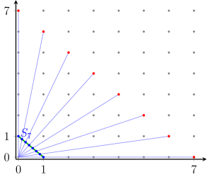
Figure 1. The discrete set $S_{k}$ (here for $k=7$) consists of the blue points sitting on the green line segment (and not of the red points).

Given $c\in\mathbb{R}$, $0<c<1$, define the set

$$\mathcal{D}_{c}=\big{\{}x\in\mathbb{R}_{+}^{d}~{}\big{|}~{}\|x\|_{1}=1,~{}c\,\mathbf{e}\leq x\big{\}}=\mathbb{S}_{\ell_{1}}\cap\big{(}\mathbb{R}^{d}_{+}+c\mathbf{e}\big{)}$$ (2.5)

as depicted in Figure 2.

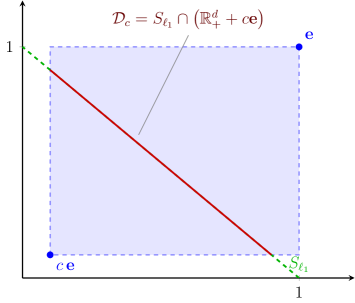
Figure 2. The set $\mathcal{D}_{c}$, here shown in dark red.

Remark 2.2.

Note that if $c>1/d$ and $c\,e\leq x$, then $\|x\|_{1}\geq cd>1$. Therefore, $\mathcal{D}_{c}$ is not empty only when $c\leq 1/d$. Also, note that if $k<d$ and $x\in S_{k}$, then $x$ must have at least one zero coordinate. Therefore, $S_{k}\cap\mathcal{D}_{c}$ is not empty only when $k\geq d$. $\diamond$

Next, we show that every point in $\mathcal{D}_{c}$ can be well approximated with a point in $S_{k}\cap\mathcal{D}_{c}$.

Proposition 2.3.

Assume that $\min\big{\{}k,\frac{1}{c}\big{\}}\geq d$. Then for every $x\in\mathcal{D}_{c}$, there exists $x_{k}\in S_{k}\cap\mathcal{D}_{c}$ such that

$$\|x-x_{k}\|_{\infty}\leq\frac{2}{k}.$$

Proof.

The set $\mathbb{S}_{\ell_{1}}$ is a simplex in $\mathbb{R}_{+}^{d}$ whose $\ell_{\infty}$ diameter is 1, i.e., the $\ell_{\infty}$ distance between any two points in $\mathbb{S}_{\ell_{1}}$ is at most 1, and it can be divided into $k^{d-1}$ simplexes, $C_{1},\dots,C_{k^{d-1}}$, whose $\ell_{\infty}$ diameter is $1/k$, cf. Figure 3. The vertices of these simplexes are the points of $S_{k}$. Let $x\in\mathcal{D}_{c}$. Then $x$ belongs to a simplex $C_{j}$ for some $j\in\{1,\dots,k^{d-1}\}$, and $C_{j}$ has $\ell_{\infty}$ diameter $1/k$. If one of the vertices of $C_{j}$ lies inside $\mathcal{D}_{c}$, then since the diameter of $C_{j}$ is $1/k$, we found a point in $S_{k}\cap\mathcal{D}_{c}$ such that $\|x-x_{k}\|_{\infty}\leq 1/k$. If this is not the case, then there must be a simplex which is adjacent to $C_{j}$ which has at least one vertex which lies in $\mathcal{D}_{c}$, cf. Figure 3.

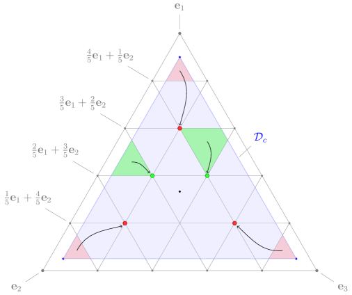
Figure 3. For the case $d=3$ the simplex $S_{\ell_{1}}$ is the convex hull of the standard unit vectors $\mathbf{e}_{1}$, $\mathbf{e}_{2}$, and $\mathbf{e}_{3}$ in $\mathbb{R}^{3}_{+}$. The points on the set $S_{k}$ (here for $k=5$) are shown in grey, and the set $\mathcal{D}_{c}$ is shown in blue. While points in the green shaded simplexes intersected with $\mathcal{D}_{c}$ can be mapped to a vertex that is in $\mathcal{D}_{c}$, this is not the case for the “corners” of the simplex $\mathcal{D}_{c}$ shown in red. The closest grid point for points $x$ near the vertices of $\mathcal{D}_{c}$ can be taken to be the opposing vertex of the neighboring simplex that shares the face intersecting $\mathcal{D}_{c}$. The distance to this vertex is always less than $2/k$ when the diameter of the simplexes $C_{j}$ is $1/k$.

Since the $\ell_{\infty}$ distance between any two points in adjacent simplexes is at most $2/k$, the result follows. ∎

We are now in a position to state and prove the main result.

Theorem 2.2.

Let $A:\mathbb{Z}_{+}^{d}\to\mathbb{Z}_{+}^{d}$ and $k\in\mathbb{N}$ is such that $k\geq d$. Assume that there exists $L\in[0,\infty)$ such that for all $x,y\in\mathbb{Z}_{+}^{d}$ with $\|x\|_{1}=\|y\|_{1}=k$,

$$d_{\mathbb{H}}(Ax,Ay)\leq L\,d_{\mathbb{H}}(x,y).$$ (2.6)

Assume also that there exists $c\in(0,1/d]$ such that for all $x\in\mathbb{Z}_{+}^{d}$ with $\|x\|_{1}=k$,

$$0<c\|Ax\|_{1}\mathbf{e}\leq Ax.$$ (2.7)

Then there exists $y_{k}\in\mathbb{Z}_{+}^{d}$ with $\|y_{k}\|_{1}=k$ satisfying

$$\left\|\frac{Ay_{k}}{\|Ay_{k}\|_{1}}-\frac{y_{k}}{\|y_{k}\|_{1}}\right\|_{2}\leq\frac{4Ldc^{-2}+2\sqrt{d}}{k}.$$ (2.8)

Inequality (2.8) says that when $\|y_{k}\|=k$ is large, the vectors $y_{k}$ and $Ay_{k}$ are ‘almost’ in the same direction, making $y_{k}$ an ‘approximate’ eigenvector of $A$, cf., Figure 4.

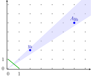
Figure 4. The point $y_{k}$ and its image $Ay_{k}$ lying in the same ‘narrow’ cone.

Proof of Theorem 2.2.

Note first that if $d=1$, since $Ax\geq c\|Ax\|_{1}\mathbf{e}>0$, it follows that for every $y\in\mathbb{N}$, we have $Ay/\|Ay\|_{1}=y/\|y\|_{1}=1$. Thus, the bound (2.8) holds trivially. Assume then that $d\geq 2$. Let $B_{k}:S_{k}\to\mathbb{S}_{\ell_{1}}$ be defined as follows,

$$B_{k}x=\frac{A(kx)}{\|A(kx)\|_{1}},$$ (2.9)

where we note that $\|A(kx)\|_{1}\neq 0$ due to (2.7). Also, $B_{k}$ is well defined since $kx\in\mathbb{Z}_{+}^{d}$ whenever $x\in S_{k}$. It is known that the Hilbert metric (2.2) is invariant under dilation, cf. [LN12]*Prop. 2.1.1, that is, if $x,y\in\mathbb{R}_{+}^{d}$ and $\alpha,\beta\in(0,\infty)$, then

$$d_{\mathbb{H}}(\alpha x,\beta y)=d_{\mathbb{H}}(x,y).$$ (2.10)

Assume that $x,y\in S_{k}$. We compute

$$d_{\mathbb{H}}(B_{k}x,B_{k}y)=d_{\mathbb{H}}\left(\frac{A(kx)}{\|A(kx)\|_{1}},\frac{A(ky)}{\|A(ky)\|_{1}}\right)\\ \stackrel{{\scriptstyle\eqref{dist invariance}}}{{=}}d_{\mathbb{H}}\big{(}A(kx),A(ky)\big{)}\stackrel{{\scriptstyle\eqref{contract prop}}}{{\leq}}Ld_{\mathbb{H}}(kx,ky)\stackrel{{\scriptstyle\eqref{dist invariance}}}{{=}}Ld_{\mathbb{H}}(x,y).$$ (2.11)

By Remark 2.2, if we assume that $k\geq d$, then $S_{k}\cap\mathcal{D}_{c}\neq\emptyset$. Let $x,y\in S_{k}\cap\mathcal{D}_{c}$. Using (2.4) and (2.11) with $\alpha=c$, $\beta=1$, we obtain

$$\|B_{k}x-B_{k}y\|_{2}\stackrel{{\scriptstyle\eqref{equiv dist 2}}}{{\leq}}\sqrt{d}\,d_{\mathbb{H}}(B_{k}x,B_{k}y)\stackrel{{\scriptstyle\eqref{B is lip}}}{{\leq}}L\sqrt{d}\,d_{\mathbb{H}}(x,y)\stackrel{{\scriptstyle\eqref{equiv dist 2}}}{{\leq}}\frac{2L\sqrt{d}}{c^{2}}\|x-y\|_{2}.$$ (2.12)

This means that $B_{k}$ is Lipschitz on $S_{k}\cap\mathcal{D}_{c}$ with respect to the Euclidean metric. Next, we study the invariance properties of $B_{k}$. Since it was assumed that $c\|Ax\|_{1}\mathbf{e}\leq Ax$, we have that $B_{k}x\geq c\,\mathbf{e}$, hence $B_{k}(S_{k})\subseteq\mathcal{D}_{c}$, and so $B_{k}\big{(}S_{k}\cap\mathcal{D}_{c}\big{)}\subseteq\mathcal{D}_{c}$ . The set $\mathcal{D}_{c}$ is compact and convex since it is the intersection of two compact convex sets. By (2.12), $B_{k}$ is Lipschitz on $S_{k}\cap\mathcal{D}_{c}$ with respect to the Euclidean metric. Therefore, by Theorem 2.1 and Remark 2.1, it follows that there exists a map $\tilde{B}_{k}:\mathcal{D}_{c}\to\mathcal{D}_{c}$ such that for all $x,y\in\mathcal{D}_{c}$,

$$\|\tilde{B}_{k}x-\tilde{B}_{k}y\|_{2}\leq\frac{2L\sqrt{d}}{c^{2}}\|x-y\|_{2}.$$ (2.13)

In particular, the map $\tilde{B}_{k}$ is a continuous map on a convex and compact set. Thus, by the Brouwer Fixed Point Theorem, there exists $\bar{x}_{k}\in\mathcal{D}_{c}$ such that $\bar{x}_{k}=\tilde{B}_{k}\bar{x}_{k}$. By Proposition 2.3, there exists $x_{k}\in S_{k}\cap\mathcal{D}_{c}$ such that $\|\bar{x}-x_{k}\|_{\infty}\leq 2/k$. Since $\|x\|_{2}\leq\sqrt{d}\|x\|_{\infty}$ for all $x\in\mathbb{R}^{d}$, it follows that

$$\|\bar{x}_{k}-x_{k}\|_{2}\leq\frac{2\sqrt{d}}{k}.$$ (2.14)

Therefore,

$$\left\|\frac{A(kx_{k})}{\|A(kx_{k})\|_{1}}-\bar{x}_{k}\right\|_{2}=\|B_{k}x_{k}-\bar{x}_{k}\|_{2}\stackrel{{\scriptstyle(*)}}{{=}}\|\tilde{B}_{k}x_{k}-\tilde{B}_{k}\bar{x}_{k}\|_{2}\stackrel{{\scriptstyle\eqref{tilde B lip}}}{{\leq}}\frac{2L\sqrt{d}}{c^{2}}\|x_{k}-\bar{x}_{k}\|_{2}\stackrel{{\scriptstyle\eqref{dist to fixed pt}}}{{\leq}}\frac{4Ld}{c^{2}k},$$

where in ($*$) we used the fact that $\tilde{B}_{k}=B_{k}$ on $S_{k}$ and $\tilde{B}_{k}\bar{x}_{k}=\bar{x}_{k}$. Altogether,

$$\left\|\frac{A(kx_{k})}{\|A(kx_{k})\|_{1}}-x_{k}\right\|_{2}\leq\left\|\frac{A(kx_{k})}{\|A(kx_{k})\|_{1}}-\bar{x}_{k}\right\|_{2}+\|\bar{x}_{k}-x_{k}\|_{2}\leq\frac{4Ld}{c^{2}k}+\frac{2\sqrt{d}}{k}=\frac{4Ldc^{-2}+2\sqrt{d}}{k}.$$

Choosing $y_{k}=kx_{k}$ proves (2.8) and this completes the proof of Theorem 2.2. ∎

We make the following remarks regarding Theorem 2.2 and its proof.

Remark 2.3.

A particular class of maps that Theorem 2.2 and Corollary 2.1 (see below) apply to is the class of homogeneous maps. It is known that if $A:\mathbb{R}_{+}^{d}\to\mathbb{R}_{+}^{d}$ is $r$-homogeneous for some $r>0$, that is, $A(\rho x)=\rho^{r}Ax$ for all $\rho>0$, and monotone, that is, $Ax\leq Ay$ whenever $x,y\in\mathbb{R}_{+}^{d}$ are such that $x\leq y$, then $A$ satisfies $d_{\mathbb{H}}(Ax,Ay)\leq rd_{\mathbb{H}}(x,y)$ for all $x,y\in\mathbb{R}_{+}^{d}$, cf.,  [LN12]*Cor. 2.1.4. In fact, it is enough to assume that the map is $r$-subhomogeneous, that is, $A(\rho x)\leq\rho^{r}Ax$ for all $\rho\geq 0$. Clearly the same is true for integer maps. $\diamond$

Remark 2.4.

For every $k\in\mathbb{N}$, $x_{k}$ can be chosen to be in the set $\big{\{}x\in\mathbb{R}^{d}~{}|~{}c\,\mathbf{e}\leq x\leq\mathbf{e}\big{\}}$ (where $c\in(0,1/d]$ may or may not depend on $k$). This means $y_{k}$ can be chosen positive. $\diamond$

Remark 2.5.

Instead of the assumption that there exists $c\in(0,1/d]$ such that $Ax\geq c\|Ax\|_{1}\mathbf{e}$ for all $x\in\mathbb{Z}_{+}^{d}$, it is enough to make the weaker assumption that $Ax\geq c\|Ax\|_{1}\mathbf{e}$ whenever $x\geq c\|x\|_{1}\mathbf{e}$. All that is really needed is the invariance of the set $\mathcal{D}_{c}$ as defined in (2.5) under the map $B_{k}$. $\diamond$

Remark 2.6.

The choice of the $\ell_{1}$-norm is essential in this proof. This is because we need the set $\mathcal{D}_{c}$ to be convex in order to use the Brouwer fixed-point theorem. This is different, e.g., from the proofs in [Koh82, Kra86], where any norm can be used. $\diamond$

Remark 2.7.

In many cases, one considers a map which is a contraction under the Hilbert metric, that is, $d_{\mathbb{H}}(Ax,Ay)<d_{\mathbb{H}}(x,y)$, and then proceeds to use the Banach contraction principle rather than the Brouwer fixed-point theorem. As a result, one obtains the “power method” for the computation of the Perron vector, i.e., that there exists $\overline{x}\in\mathbb{R}_{+}^{d}$, $\|\overline{x}\|=1$, such that for all $x\in\mathbb{R}_{+}^{d}\setminus\{0\}$, $A^{n}x/\|A^{n}x\|\stackrel{{\scriptstyle n\to\infty}}{{\longrightarrow}}\overline{x}$. However, since in Theorem 2.2 Kirszbraun’s extension theorem is used, the extended map is typically not a contraction and therefore this power method does not hold. $\diamond$

Next, it is shown that if we have good bounds on the norm of $Ax$ for $x\in\mathbb{Z}_{+}^{d}$, then we can find a sequence $\{y_{k}\}_{k=1}^{\infty}\subseteq\mathbb{Z}_{+}^{d}$ with a controlled behavior in the following sense.

Corollary 2.1.

Let $A:\mathbb{Z}_{+}^{d}\to\mathbb{Z}_{+}^{d}$ and $k\in\mathbb{N}$ is such that $k\geq d$. Assume that there exists $L\in[0,\infty)$ such that for all $x,y\in\mathbb{Z}_{+}^{d}$ with $\|x\|_{1}=\|y\|_{1}=k$,

$$d_{\mathbb{H}}(Ax,Ay)\leq Ld_{\mathbb{H}}(x,y).$$

Let us assume that there exists $c\in(0,1/d]$ such that for all $x\in\mathbb{Z}_{+}^{d}$ with $\|x\|_{1}=k$,

$$0<c\|Ax\|_{1}\mathbf{e}\leq Ax.$$

Assume also that there exists $a\in(0,\infty)$ such that $\|Ax\|_{1}\geq a\|x\|_{1}$ for all $x\in\mathbb{Z}_{+}^{d}$ with $\|x\|_{1}=k$. Then there exists $y_{k}\in\mathbb{Z}_{+}^{d}$ with $\|y_{k}\|_{1}=k$ such that

$$a\left(1-\frac{4Ldc^{-2}+2\sqrt{d}}{ck}\right)y_{k}\leq Ay_{k}.$$ (2.15)

Alternatively, assume that there exists $b\in(0,\infty)$ such that $\|Ax\|_{1}\leq b\|x\|_{1}$ for all $x\in\mathbb{Z}_{+}^{d}$ with $\|x\|_{1}=k$. Then there exists $y_{k}\in\mathbb{Z}_{+}^{d}$ with $\|y_{k}\|_{1}=k$ such that

$$Ay_{k}\leq b\left(1+\frac{4Ldc^{-2}+2\sqrt{d}}{ck}\right)y_{k}.$$ (2.16)

In both cases, we have $\|y_{k}\|_{1}=k$. In particular, if $Ax\geq c\|Ax\|_{1}\mathbf{e}$ and $\|Ax\|_{1}\geq a\|x\|_{1}$ ($0<\|Ax\|_{1}\leq b\|x\|_{1}$) for all $x\in\mathbb{Z}_{+}^{d}\setminus\{0\}$, then there exists a sequence $\{y_{k}\}_{k=1}^{\infty}\subseteq\mathbb{Z}_{+}^{d}$ such that for every $\varepsilon>0$, there exists $k_{0}\in\mathbb{N}$ such that for every $k\geq k_{0}$, $Ay_{k}\geq a(1-\varepsilon)y_{k}$ (respectively, $Ay_{k}\leq b(1+\varepsilon)y_{k}$).

Proof.

By Theorem 2.2, there exists $y_{k}\in\mathbb{Z}_{+}^{d}$ with $\|y_{k}\|_{1}=k$ such that $\|Ay_{k}\|_{1}\neq 0$ and

$$\left\|\frac{Ay_{k}}{\|Ay_{k}\|_{1}}-\frac{y_{k}}{\|y_{k}\|_{1}}\right\|_{\infty}\leq\left\|\frac{Ay_{k}}{\|Ay_{k}\|_{1}}-\frac{y_{k}}{\|y_{k}\|_{1}}\right\|_{2}\leq\frac{4Ldc^{-2}+2\sqrt{d}}{k}.$$

In particular, it follows that

$$-\left(\frac{4Ldc^{-2}+2\sqrt{d}}{k}\right)\mathbf{e}\leq\frac{Ay_{k}}{\|Ay_{k}\|_{1}}-\frac{y_{k}}{\|y_{k}\|_{1}}\leq\left(\frac{4Ldc^{-2}+2\sqrt{d}}{k}\right)\mathbf{e},$$

and so

$$\|A(y_{k})\|_{1}\left(\frac{y_{k}}{\|y_{k}\|_{1}}-\frac{4Ldc^{-2}+2\sqrt{d}}{k}\,\mathbf{e}\right)\leq A(y_{k})\leq\|A(y_{k})\|_{1}\left(\frac{y_{k}}{\|y_{k}\|_{1}}+\frac{4Ldc^{-2}+2\sqrt{d}}{k}\,\mathbf{e}\right).$$

By Remark 2.4, if $x_{k}=y_{k}/\|y_{k}\|_{1}=y_{k}/k$, then $c\,\mathbf{e}\leq x_{k}\leq\mathbf{e}$ and so $\mathbf{e}\leq\frac{1}{c}x_{k}=\frac{1}{ck}y_{k}$. Hence,

$$\left(1-\frac{4Ldc^{-2}+2\sqrt{d}}{ck}\right)\frac{\|Ay_{k}\|_{1}y_{k}}{\|y_{k}\|_{1}}\leq Ay_{k}\leq\left(1+\frac{4Ldc^{-2}+2\sqrt{d}}{ck}\right)\frac{\|Ay_{k}\|_{1}y_{k}}{\|y_{k}\|_{1}}.$$

Assume that $\|Ax\|_{1}\geq a\|x\|_{1}$ for all $x\in\mathbb{Z}_{+}^{d}$ with $\|x\|_{1}=k$. Then

$$Ay_{k} \geq\left(1-\frac{4Ldc^{-2}+2\sqrt{d}}{ck}\right)\frac{\|Ay_{k}\|_{1}y_{k}}{\|y_{k}\|_{1}}\geq a\left(1-\frac{4Ldc^{-2}+2\sqrt{d}}{ck}\right)y_{k},$$

which proves (2.15). Alternatively, assuming that $\|Ax\|_{1}\leq b\|x\|_{1}$ for all $x\in\mathbb{Z}_{+}^{d}$ with $\|x\|_{1}=k$,

$$Ay_{k} \leq\left(1+\frac{4Ldc^{-2}+2\sqrt{d}}{ck}\right)\frac{\|Ay_{k}\|_{1}y_{k}}{\|y_{k}\|_{1}}\leq b\left(1+\frac{4Ldc^{-2}+2\sqrt{d}}{ck}\right)y_{k},$$

which proves (2.16), and completes the proof. ∎

Remark 2.8.

In the case we can choose $a=1$ for all $k\in\mathbb{N}$ or $b=1$ for all $k\in\mathbb{N}$, Corollary 2.1 gives a sequence $\{y_{k}\}_{k=1}^{\infty}\subseteq\mathbb{Z}_{+}^{d}$ on which $A$ is ‘almost monotone’. That is, if $a=1$, then there exists a sequence $\{y_{k}\}_{k=1}^{\infty}\subseteq\mathbb{Z}_{+}^{d}$ such that for every $\varepsilon>0$, there exists $k_{0}\in\mathbb{N}$ such that for all $k\geq k_{0}$, $(1-\varepsilon)y_{k}\leq Ay_{k}$. This is close to a monotonicity property $y_{k}\leq Ay_{k}$. Similarly in the case where $b=1$, we obtain a sequence $\{y_{k}\}_{k=1}^{\infty}\subseteq\mathbb{Z}_{+}^{d}$ with $\|y_{k}\|_{1}=k$ such that $Ay_{k}\leq(1+\varepsilon)y_{k}$ for $k$ sufficiently large. $\diamond$

3. Concave maps on integer lattices

Recall that a map $F:\mathbb{R}^{d}_{+}\to\mathbb{R}_{+}^{d}$ is said to be concave if for every $x,y\in\mathbb{R}_{+}^{d}$ and every $\alpha\in[0,1]$,

$$F(\alpha x+(1-\alpha)y)\geq\alpha Fx+(1-\alpha)Fy.$$

The notion of concavity can also be studied in $\mathbb{Z}_{+}^{d}$, cf. [BG18].

Definition 3.1.

A map $A:\mathbb{Z}_{+}^{d_{1}}\to\mathbb{Z}_{+}^{d_{2}}$ is said to be concave if for every $x,x_{1},\dots,x_{n}\in\mathbb{Z}_{+}^{d_{1}}$ and $m,m_{1},\dots,m_{n}\in\mathbb{N}$ such that $mx=\sum_{i=1}^{n}m_{i}x_{i}$ and $m=\sum_{i=1}^{n}m_{i}$ we have

$$mAx\geq\sum_{i=1}^{n}m_{i}Ax_{i}.$$ (3.1)

A map $A:\mathbb{Z}_{+}^{d_{1}}\to\mathbb{Z}_{+}^{d_{2}}$ is said to be affine if in (3.1) we have an equality rather than an inequality.

The following result follows directly from Theorem 1 and Corollary 2 in [PW86]. It shows that every concave map on $\mathbb{Z}_{+}^{d}$ can be extended to a concave map on $\mathbb{R}_{+}^{d}$.

Theorem 3.1 ([PW86]).

Assume that $A:\mathbb{Z}_{+}^{d}\to\mathbb{Z}_{+}^{d}$ is concave. Then there exists $F:\mathbb{R}_{+}^{d}\to\mathbb{R}_{+}^{d}$ concave such that $F\big{|}_{\mathbb{Z}_{+}^{d}}=A$.

As a result, the following holds.

Proposition 3.1.

Assume that $A:\mathbb{Z}_{+}^{d}\to\mathbb{Z}_{+}^{d}$ is concave and that $x,y\in\mathbb{Z}_{+}^{d}$ are such that $\|x\|_{1}=\|y\|_{1}>0$. Then $A$ is $d_{\mathbb{H}}$-nonexpansive, that is

$$d_{\mathbb{H}}(Ax,Ay)\leq d_{\mathbb{H}}(x,y).$$

Proof.

By Theorem 3.1 there exists $F:\mathbb{R}_{+}^{d}\to\mathbb{R}_{+}^{d}$ concave such that $Fx=Ax$ for all $x\in\mathbb{Z}_{+}^{d}$. Assume that $m,n\in\mathbb{Z}_{+}$ are such that $mx\leq ny$. Since $\|x\|_{1}=\|y\|_{1}$, it follows that $m\leq n$. Hence, there exists $z\in\mathbb{R}_{+}^{d}$ such that

$$ny=mx+(n-m)z.$$ (3.2)

Since $F:\mathbb{R}_{+}^{d}\to\mathbb{R}_{+}^{d}$ is concave and positive,

$$nFy\geq mFx+(n-m)Fz\geq mFx.$$

Since $F\big{|}_{\mathbb{Z}_{+}^{d}}=A$, it follows that $nAy\geq mAx$. Thus, by (2.1), $\lambda(Ax,Ay)\geq\lambda(x,y)$. Similarly, $\lambda(Ay,Ax)\geq\lambda(y,x)$. Therefore, by the definition of the Hilbert metric (2.2), $d_{\mathbb{H}}(Ax,Ay)\leq d_{\mathbb{H}}(x,y)$, and this completes the proof. ∎

Example 3.1.

In (3.2) one cannot assume $z$ to be in $\mathbb{Z}^{d}_{+}$. E.g., for $x=(1,1,3)$ and $y=(2,2,1)$ we verify $\|x\|_{1}=\|y\|_{1}=5$ and have $\lambda(x,y)=\min_{i}\frac{y_{i}}{x_{i}}=\frac{1}{3}$, so $mx\leq ny$ holds with $m=1$ and $n=3$. Hence, $(n-m)=2$ and the vector $z$ defined by (3.2) has to be $\big{(}\frac{5}{2},\frac{5}{2},0\big{)}$.

Remark 3.1.

Proposition 3.1 remains true if $A$ is a supremum of concave maps. However, this does not mean that Proposition 3.1 holds for convex maps. Indeed, any convex map $F:\mathbb{R}_{+}^{d}\to\mathbb{R}_{+}^{d}$ can be written as $F=\sup_{t\in\mathcal{T}}F_{t}$, where $\{F_{t}\}_{t\in\mathcal{T}}$ is a family of affine—and in particular concave—maps. If $\|x\|_{1}=\|y\|_{1}$ and $mx\leq ny$, then as before we get $ny=mx+(n-m)z$ for some $z\in\mathbb{R}_{+}^{d}$. However, there is no guarantee that $F_{t}z\geq 0$, that is, $F_{t}$ does not necessarily map $\mathbb{R}_{+}^{d}$ to $\mathbb{R}_{+}^{d}$. Therefore, in general, Proposition 3.1 does not hold for convex maps. $\diamond$

Using Proposition 3.1 and Remark 3.1, we conclude the following.

Theorem 3.2.

Assume that $A_{t}:\mathbb{Z}_{+}^{d}\to\mathbb{Z}_{+}^{d}$, $t\in\mathcal{T}$, are concave maps and $k\in\mathbb{N}$ is such that $k\geq d$. Assume also there exist $c\in(0,1/d]$ such that $0<c\|A_{t}x\|_{1}\mathbf{e}\leq A_{t}x$ for all $t\in\mathcal{T}$ and $x\in\mathbb{Z}_{+}^{d}$ with $\|x\|_{1}=k$. Let $A=\sup_{t\in\mathcal{T}}A_{t}$. Then there exists $y_{k}\in\mathbb{Z}_{+}^{d}$ with $\|y_{k}\|_{1}=k$ such that

$$\left\|\frac{Ay_{k}}{\|Ay_{k}\|_{1}}-\frac{y_{k}}{\|y_{k}\|_{1}}\right\|_{2}\leq\frac{4dc^{-2}+2\sqrt{d}}{k}.$$ (3.3)

If there exists $b\in(0,\infty)$ such that $\|Ax\|_{1}\leq b\|x\|_{1}$ for all $x\in\mathbb{Z}_{+}^{d}$ with $\|x\|_{1}=k$, Then there exists $y_{k}\in\mathbb{Z}_{+}^{d}$ with $\|y_{k}\|_{1}=k$ such that

$$Ay_{k}\leq b\left(1+\frac{4dc^{-2}+2\sqrt{d}}{ck}\right)y_{k}.$$ (3.4)

If there exists $a\in(0,\infty)$ such that $\|A_{t_{0}}x\|_{1}\geq a\|x\|_{1}$ for some $t_{0}\in\mathcal{T}$ and all $x\in\mathbb{Z}_{+}^{d}$ with $\|x\|_{1}=k$, then there exists $y_{k}\in\mathbb{Z}_{+}^{d}$ with $\|y_{k}\|_{1}=k$ and

$$Ay_{k}\geq a\left(1-\frac{4dc^{-2}+2\sqrt{d}}{ck}\right)y_{k}.$$ (3.5)

Proof.

Since $A=\sup_{t\in\mathcal{T}}A_{t}$, by Remark 3.1 it follows that $d_{\mathbb{H}}(Ax,Ay)\leq d_{\mathbb{H}}(x,y)$ for all $x,y\in\mathbb{Z}_{+}^{d}$ with $\|x\|_{1}=\|y\|_{1}=k$. Hence, Theorem 2.2 holds with $L=1$, which proves (3.3). Next, if $\|Ax\|_{1}\leq b\|x\|_{1}$ for all $x\in\mathbb{Z}_{+}^{d}$ with $\|x\|_{1}=k$, then using Corollary 2.1 proves (3.4). Finally, if $\|A_{t_{0}}x\|\geq a\|x\|_{1}$ for some $t_{0}\in\mathcal{T}$ and all $x\in\mathbb{Z}_{+}^{d}$, $\|x\|_{1}=k$, then $\|Ax\|_{1}\geq\|A_{t_{0}}x\|_{1}\geq a\|x\|_{1}$. Therefore, again by using Corollary 2.1, (3.5) follows, and this completes the proof. ∎

Remark 3.2.

The reader might wonder why the previous proof is not based on Banach’s contraction principle, given the Lipschitz bound for $A$ is bounded by $1$. The reason is that due to the extension via Kirszbraun’s extension theorem—which requires the Euclidean norm and hence constants from the norm equivalence get introduced—the Lipschitz constant for the resulting extended map is not necessarily bounded above by $1$ anymore. As a result, there seems little hope that without additional assumptions the result could be proven by appealing to Banach’s contraction principle. $\diamond$

Remark 3.3.

The authors were made aware by a referee that a concave map $f\colon\mathbb{Z}^{d}\to\mathbb{Z}^{d}$ is nonexpansive under Thompson’s metric,

$$d_{\mathbb{T}}(x,y)=\begin{dcases}-\log\min\big{\{}\lambda(x,y),\lambda(y,x)\big{\}}&\text{for }\min\big{\{}\lambda(x,y),\lambda(y,x)\big{\}}>0,\\ \infty&\text{otherwise,}\end{dcases}$$

and would like to thank the referee for pointing out the following details which provide a useful alternative to proving results like Theorem 3.2.

Indeed, if $d_{\mathbb{T}}(x,y)=-\log\lambda(x,y)=-\log\min_{i}\frac{y_{i}}{x_{i}}=\log\frac{m}{n}$, then $m\geq n$, as $d_{\mathbb{T}}(x,y)\geq 0$. Thus, $\frac{n}{m}x\leq y$ and $\frac{n}{m}y\leq x$. Now concavity gives $nf(x)\geq f(nx)+(n-1)f(0)\geq f(nx)$ and likewise $mf(y)\geq f(my)$.

Recall that $nx\leq my$, so that if we write $my=nx+(m-n)z$, we deduce that $z\in\mathbb{R}^{d}_{+}$. As in the proof of Proposition 3.1, this implies that the extension $F\colon\mathbb{R}^{d}_{+}\to\mathbb{R}^{d}_{+}$ of $f$ given by Theorem 3.1 satisfies $mF(y)\geq n(F(x)+(n-m)F(z)\geq nF(x)$, so that $mf(y)\geq nf(x)$. Thus we have $\lambda(f(x),f(y))\geq\frac{n}{m}$. Using $\frac{n}{m}y\leq x$ it can be shown in the same way that $\lambda(f(y),f(x))\geq\frac{n}{m}$. Thus $d_{\mathbb{T}}(f(x),f(y))\leq d_{T}(x,y)$ for all $x,y\in\mathbb{Z}^{d}$.

Now as $\big{(}\text{int\,}\mathbb{R}_{+}^{d},d_{\mathbb{T}}\big{)}$ is isometric to $\big{(}\mathbb{R}^{d},\|\cdot\|_{\infty}\big{)}$ (component-wise $\log$ is an isometry, c.f. [LN12]*Prop. 2.2.1), and every sup-norm nonexpansive map on subset of $\mathbb{R}^{d}$ can be extended in a nonexpansive way to the whole $\mathbb{R}^{d}$, c.f. [LN12]*Lem. 4.2.4, we find that $f\colon\mathbb{Z}_{+}^{d}\to\mathbb{Z}_{+}^{d}$ can be extended into a $d_{\mathbb{T}}$-nonexpansive way to $\mathbb{R}^{d}_{+}$. More details can be found in [LN12]*Ch. 4.  $\diamond$

It is known that a minimum of affine maps is concave (see [BG18]). As an immediate corollary of Theorem 3.2, we obtain the following results for a ‘zigzag’ map, that is, a map which is a maximum of minima of a finite number of affine maps.

Corollary 3.1.

Assume that $A_{i,j}:\mathbb{Z}_{+}^{d}\to\mathbb{Z}_{+}^{d}$, $i\in\{1,\dots,I\}$, $j\in\{1,\dots,J\}$ are affine maps, where $I,J\in\mathbb{N}$, and $k\in\mathbb{N}$ is such that $k\geq d$. Assume also that there exists $c\in(0,1/d]$ such that $0<c\|A_{i,j}x\|_{1}e\leq A_{i,j}x$ for all $x\in\mathbb{Z}_{+}^{d}$ with $\|x\|_{1}=k$ and for all $i\in\{1,\dots,I\}$, $j\in\{1,\dots,J\}$. Define $A:\mathbb{Z}_{+}^{d}\to\mathbb{Z}_{+}^{d}$ by

$$A=\max_{i\in\{1,\dots,I\}}\min_{j\in\{1,\dots,J\}}A_{i,j}.$$

Then there exists $y_{k}\in\mathbb{Z}_{+}^{d}$ with $\|y_{k}\|_{1}=k$ such that

$$\left\|\frac{Ay_{k}}{\|Ay_{k}\|_{1}}-\frac{y_{k}}{\|y_{k}\|_{1}}\right\|_{2}\leq\frac{4dc^{-2}+2\sqrt{d}}{k}.$$

Also, if there exists $b\in(0,\infty)$ such that $0<\|Ax\|_{1}\leq b\|x\|_{1}$ for all $x\in\mathbb{Z}_{+}^{d}$ with $\|x\|_{1}=k$, then there exists $y_{k}\in\mathbb{Z}_{+}^{d}$ with $\|y_{k}\|_{1}=k$ such that

$$Ay_{k}\leq b\left(1+\frac{4dc^{-2}+2\sqrt{d}}{ck}\right)y_{k}.$$

If, in addition, there exists $a\in(0,\infty)$ such that $a\|x\|_{1}\leq\|\min_{j\in\{1,\dots,J\}}A_{i_{0},j}x\|_{1}$ for some $i_{0}\in\{1,\dots,I\}$ and all $x\in\mathbb{Z}_{+}^{d}$ with $\|x\|_{1}=k$, then there exists $y_{k}\in\mathbb{Z}_{+}^{d}$ with $\|y_{k}\|_{1}=k$ such that

$$Ay_{k}\geq a\left(1-\frac{4dc^{-2}+2\sqrt{d}}{ck}\right)y_{k}.$$

Next, it is shown that any concave map on $\mathbb{Z}_{+}^{d}$ has a controlled growth rate, that is, there is always $b\in(0,\infty)$ such that $\|Ax\|_{1}\leq b\|x\|_{1}$. This is similar to the case of concave maps on $\mathbb{R}_{+}^{d}$.

Proposition 3.2.

Assume that $A:\mathbb{Z}_{+}^{d}\to\mathbb{Z}_{+}^{d}$ is concave. Then there exists $b^{\prime}\in(0,\infty)$ such that for all $x\in\mathbb{Z}_{+}^{d}\setminus\{0\}$,

$$\|Ax\|_{1}\leq\big{(}\|A(0)\|_{1}+b^{\prime}d\big{)}\|x\|_{1}.$$

Proof.

First, we would like to show that $Ax\geq A(0)$ for all $x\in\mathbb{Z}_{+}^{d}$. Indeed, write $A=(A_{1},\dots,A_{d})$, where $A_{i}:\mathbb{Z}_{+}^{d}\to\mathbb{Z}_{+}$, $i\in\{1,\dots,d\}$, are concave. Assume that we dot not have $Ax\geq A(0)$ for all $x\in\mathbb{Z}_{+}^{d}$. Then without loss of generality assume that $A_{1}x<A_{1}(0)$ for some $x\in\mathbb{Z}_{+}^{d}$. Since for all $k\in\mathbb{N}$, $kx=1\cdot(kx)+(k-1)\cdot 0$ and since $A_{1}$ is concave,

$$A_{1}(kx)\leq k(A_{1}x-A_{1}(0))+A_{1}(0).$$

If $k$ is sufficiently large, then we must have $A_{1}(kx)<0$ which is a contradiction to the assumption that $A$ is positive. This also means that the map $A-A(0)$ is a concave map and $Ax-A(0)\in\mathbb{Z}_{+}^{d}$ for all $x\in\mathbb{Z}_{+}^{d}$. By Theorem 3.1, there exists $F:\mathbb{R}_{+}^{d}\to\mathbb{R}_{+}^{d}$ concave such that $F\big{|}_{\mathbb{Z}_{+}^{d}}=A-A(0)$. Note that $F(0)=0$. It is known that in such case there exists $b^{\prime}\in(0,\infty)$ such that $F(x/\|x\|_{1})\leq b^{\prime}\,\mathbf{e}$, cf., e.g., [Kra86]*p. 281. Let $x\in\mathbb{Z}_{+}^{d}\setminus\{0\}$. Then we must have $\|x\|_{1}\geq 1$. Hence, by the concavity of $F$ and the fact that $F(0)=A(0)-A(0)=0$,

$$F\left(\frac{x}{\|x\|_{1}}\right)\geq\frac{1}{\|x\|_{1}}Fx+\left(1-\frac{1}{\|x\|_{1}}\right)F(0)=\frac{Fx}{\|x\|_{1}}.$$

Hence, we have $Fx\leq b^{\prime}\|x\|_{1}\mathbf{e}$. Since $Fx=Ax-A(0)$ for all $x\in\mathbb{Z}_{+}^{d}$ and since $\|\mathbf{e}\|_{1}=d$, it follows that

$$\|Ax\|_{1}\leq\|A(0)\|_{1}+\|Fx\|_{1}\leq\|A(0)\|_{1}+b^{\prime}d\|x\|_{1}\leq\big{(}\|A(0)\|_{1}+b^{\prime}d\big{)}\|x\|_{1},$$

which completes the proof. ∎

Remark 3.4.

Proposition 3.2 is by no means optimal. In particular, for some $k\in\mathbb{N}$, we might find $b\in(0,\infty)$ much smaller than $\|A(0)\|_{1}+b^{\prime}d$ such that $\|Ax\|_{1}\leq b\|x\|_{1}$ for all $x\in\mathbb{Z}_{+}^{d}$ with $\|x\|_{1}=k$. $\diamond$

Finally, we show if the image of a concave map on $\mathbb{R}_{+}^{d}$ is always rounded up to the next integer value, one obtains an integer map which has a controlled Lipschitz constant. Here for $x=(x_{1},\dots,x_{d})\in\mathbb{R}_{+}^{d}$, denote by $\lceil x\rceil$ the vector of rounded-up integer values, that is, $\big{(}\lceil x_{1}\rceil,\dots,\lceil x_{d}\rceil\big{)}$, where $\lceil r\rceil$ denotes the smallest integer that is larger than or equal to the real number $r$. This will be of use when we study the applications in Section 4.

Proposition 3.3.

Assume that $F:\mathbb{R}_{+}^{d}\to\mathbb{R}_{+}^{d}$ is concave and $k\in\mathbb{N}$. Assume also that there exist $a\in(0,\infty)$ and $c\in(0,1/d]$ such that $Fx\geq c\|Fx\|_{1}\mathbf{e}>0$ and $\|Fx\|_{1}\geq a\|x\|_{1}$ for all $x\in\mathbb{R}_{+}^{d}$ with $\|x\|_{1}=k$. Let $Ax=\lceil Fx\rceil$. Then for all $x,y\in\mathbb{Z}_{+}^{d}$ with $\|x\|_{1}=\|y\|_{1}=k$,

$$d_{\mathbb{H}}(Ax,Ay)\leq\left(1+\frac{2}{ac}\right)d_{\mathbb{H}}(x,y).$$

Proof.

Assume that $x,y\in\mathbb{Z}_{+}^{d}$ are such that $\|x\|_{1}=\|y\|_{1}=k$ and $m,n\in\mathbb{Z}_{+}$ are such that $mx\leq ny$. Then in particular it follows that $m\leq n$. As before, since $F$ is concave on $\mathbb{R}_{+}^{d}$, there exists $z\in\mathbb{R}_{+}^{d}$ such that $ny=mx+(n-m)z$ and as a result $nFy\geq mFx+(n-m)Fz\geq mFz$. Taking the ceiling function and using the fact that it is known that for every $x\in\mathbb{R}_{+}^{d}$, $x\leq\lceil x\rceil\leq x+\mathbf{e}$, gives $nAy\geq m(Ax-\mathbf{e})$. Since $Fx\geq c\|Fx\|_{1}\mathbf{e}$, it follows that

$$\frac{m}{n}Ax\leq Ay+\frac{m}{n}\mathbf{e}\stackrel{{\scriptstyle(*)}}{{\leq}}Ay+\frac{Fy}{c\|Fy\|_{1}}\stackrel{{\scriptstyle(**)}}{{\leq}}Ay+\frac{Ay}{ac\|y\|_{1}}=\left(1+\frac{1}{ac\|y\|_{1}}\right)Ay,$$ (3.6)

where in ($*$) we used the fact that $m\leq n$ and the assumption on $F$, and in ($**$) we used the fact that $Fy\leq Ay$ and $\|Fy\|_{1}\geq a\|y\|_{1}$. Altogether, by (2.1) combined with (3.6), it follows that

$$\lambda(Ax,Ay)\geq\frac{\lambda(x,y)}{1+\frac{1}{ac\|y\|_{1}}}.$$

Similarly,

$$\lambda(Ay,Ax)\geq\frac{\lambda(y,x)}{1+\frac{1}{ac\|x\|_{1}}}.$$

Therefore, by (2.2), it follows that

$$d_{\mathbb{H}}(Ax,Ay) \leq d_{\mathbb{H}}(x,y)+\log\left(1+\frac{1}{ac\|x\|_{1}}\right)+\log\left(1+\frac{1}{ac\|y\|_{1}}\right)$$

$$\stackrel{{\scriptstyle(*)}}{{\leq}}d_{\mathbb{H}}(x,y)+\frac{1}{ac\|x\|_{1}}+\frac{1}{ac\|y\|_{1}},$$ (3.7)

where in ($*$) we used the fact that $\log(1+x)\leq x$ for all $x\in\mathbb{R}_{+}$. Now, since $\|x\|_{1}=\|y\|_{1}$, it follows that $\max\{x,y\}\leq\|x\|_{1}\mathbf{e}$. Also, since $x,y\in\mathbb{Z}_{+}^{d}$, it follows that $\|x-y\|_{\infty}\geq 1$ whenever $x\neq y$. Therefore, by the right-hand inequality in (2.3), $d_{\mathbb{H}}(x,y)\geq 1/\|x\|_{1}$ and also $d_{\mathbb{H}}(z,y)\geq 1/\|y\|_{1}$. Using this in (3), it follows that

$$d_{\mathbb{H}}(Ax,Ay)\leq\left(1+\frac{2}{ac}\right)d_{\mathbb{H}}(x,y),$$

and this completes the proof. ∎

4. Applications

4.1. A discrete epidemic model

One of the oldest epidemic models is the Susceptible-Infected-Susceptible (SIS) model, which is a special case of the model studied in [KM27] and describes the infection rates in a system with several separate locations, say, different cities or countries. The continuous version of this model can be described by the following system of differential equations for $d$ different locations. For $i\in\{1,\dots,d\}$ let $x_{i}(t)\in[0,1]$ denote the portion of population at location $i$ which is infected at time $t\in\mathbb{R}_{+}$. Then $x_{i}(t)$ changes according to

$$\dot{x}_{i}(t)=-\delta_{i}x_{i}(t)+\sum_{j=1}^{d}b_{i,j}\big{[}x_{j}(t)(1-x_{i}(t))\big{]},$$ (4.1)

where $\delta_{i}\in[0,1]$ and $b_{i,j}\geq 0$, $i,j\in\{1,\dots,d\}$ are model parameters, cf., e.g., [NPP16] for more information about this and other epidemic models.

Assume now that $x_{i}\in\mathbb{Z}_{+}$ is the number of infected people at location $i$, which has a total population of $M_{i}$. Then a discrete version of (4.1) would be

$$\frac{x_{i}(n+1)}{M_{i}}-\frac{x_{i}(n)}{M_{i}}=-\delta_{i}\frac{x_{i}(n)}{M_{i}}+\sum_{j=1}^{d}b_{i,j}\frac{x_{j}(n)}{M_{j}}\left(1-\frac{x_{i}(n)}{M_{i}}\right),$$

which gives

$$x_{i}(n+1)=\delta_{i}^{\prime}x_{i}(n)+\sum_{j=1}^{d}b_{i,j}\frac{x_{j}(n)}{M_{j}}\big{(}M_{i}-x_{i}(n)\big{)},$$

with $\delta_{i}^{\prime}=1-\delta_{i}\in[0,1]$. In the discrete setting, it is therefore natural to consider the difference equation $x(n+1)=A(x(n))$ where $n\in\mathbb{Z}_{+}$, and for $i\in\{1,\dots,d\}$, $A_{i}:\mathbb{Z}_{+}^{d}\to\mathbb{Z}_{+}$ is given by

$$A_{i}x=\min\big{\{}M_{i},\lceil P_{i}x\rceil\big{\}},$$ (4.2)

with $P_{i}:\mathbb{R}^{d}\to\mathbb{R}$ being the (approximate) infected population, which is given by

$$P_{i}x=\delta_{i}^{\prime}x_{i}+\sum_{j=1}^{d}b_{i,j}\frac{x_{j}}{M_{j}}\big{(}M_{i}-x_{i}\big{)},$$ (4.3)

where $\delta_{i}^{\prime},b_{i,j}\in\mathbb{R}_{+}$. The choice of a ceiling function in (4.2) rather than a floor function is not particularly important. It only makes some of the calculations below slightly simpler.

Next, it is shown that under certain assumptions on the coefficients of the the operators $P_{i}$, we can obtain a Lipschitz condition on the map $A$.

Proposition 4.1.

Let $A=(A_{1},\dots,A_{d})$ is the map defined in (4.2). Assume that there exist numbers $\delta_{*},\delta^{*},B_{*},B^{*},R_{*},R^{*}\in(0,\infty)$ such that for all $i,j\in\{1,\dots,d\}$,

$$\delta_{*} \leq\;\delta_{i}^{\prime} \leq\delta^{*},$$ (4.4)

$$B_{*} \leq b_{i,j} \leq B^{*},$$ (4.5)

$$R_{*} \leq\dfrac{M_{i}}{M_{j}} \leq R^{*}.$$ (4.6)

Assume that $k\in\mathbb{N}$ is such that

$$k\leq\min\{M_{1},\dots,M_{d}\}.$$ (4.7)

Then for every $x=(x_{1},\dots,x_{d})\in\mathbb{Z}_{+}^{d}$ with $\|x\|_{1}=k$ and $x_{i}\leq M_{i}$ for all $i\in\{1,\dots,d\}$,

$$\frac{1}{2}\min\left\{\delta_{*},R_{*}B_{*}\right\}k\mathbf{e}\leq Ax\leq\left(\delta^{*}+R^{*}B^{*}+1\right)k\mathbf{e}.$$ (4.8)

If it is assumed further that $k\in\mathbb{N}$ is such that

$$k\leq\frac{\min\{M_{1},\dots,M_{d}\}}{\delta^{*}+R^{*}B^{*}+1}.$$ (4.9)

Then for every $x,y\in\mathbb{Z}_{+}^{d}$ with $\|x\|_{1}=\|y\|_{1}=k$ and $x_{i},y_{i}\leq M_{i}$ for all $i\in\{1,\dots,d\}$,

$$d_{\mathbb{H}}(Ax,Ay)\leq\frac{4\left(\delta^{*}+R^{*}B^{*}+1\right)\left(\delta^{*}+R^{*}B^{*}d+B^{*}d+2\right)}{\min\left\{\delta_{*}^{2},R_{*}^{2}B_{*}^{2}\right\}}\,d_{\mathbb{H}}(x,y).$$ (4.10)

Proof.

Fix $i\in\{1,\dots,d\}$. If $x_{i}\geq\frac{k}{2}$, then by (4.3), $P_{i}x\geq\delta_{i}^{\prime}x_{i}\geq\frac{1}{2}\delta_{*}k$, and so $\lceil P_{i}x\rceil\geq\lceil\frac{1}{2}\delta_{*}k\rceil\geq\frac{1}{2}\delta_{*}k$. Alternatively, if $x_{i}\leq\frac{k}{2}$, then by (4.7) it follows that $1-\frac{x_{i}}{M_{i}}\geq\frac{1}{2}$, and so

$$P_{i}x\geq\sum_{j=1}^{d}b_{i,j}\frac{x_{j}}{M_{j}}\big{(}M_{i}-x_{i}\big{)}=\sum_{j=1}^{d}b_{i,j}x_{j}\frac{M_{i}}{M_{j}}\left(1-\frac{x_{i}}{M_{i}}\right)\stackrel{{\scriptstyle\eqref{bounds R}}}{{\geq}}\frac{1}{2}R_{*}\sum_{j=1}^{d}b_{i,j}x_{j}\stackrel{{\scriptstyle\eqref{bounds B}}}{{\geq}}\frac{1}{2}R_{*}B_{*}k.$$

Thus, $\lceil P_{i}x\rceil\geq\lceil\frac{1}{2}R_{*}B_{*}k\rceil\geq\frac{1}{2}R_{*}B_{*}k$. In both case, we obtain $\lceil P_{i}x\rceil\geq\frac{1}{2}\min\big{\{}\delta_{*},R_{*}B_{*}\big{\}}k$. Since $\delta_{*}\leq 1$, it follows that $M_{i}\geq\frac{1}{2}\min\left\{\delta_{*},R_{*}B_{*}\right\}$ for all $i\in\{1,\dots,d\}$, and so by the definition of $A_{i}$ in (4.2), $A_{i}x\geq\frac{1}{2}\min\left\{\delta_{*},R_{*}B_{*}\right\}$. This proves the left-hand inequality in (4.8). On the other hand, for every $i\in\{1,\dots,d\}$, we have $P_{i}x\leq\delta^{*}x_{i}+R^{*}B^{*}k\leq\left(\delta^{*}+R^{*}B^{*}\right)k$. Therefore,

$$A_{i}x\leq\lceil P_{i}x\rceil\leq P_{i}x+1\leq\left(\delta^{*}+R^{*}B^{*}\right)k+1\leq\left(\delta^{*}+R^{*}B^{*}+1\right)k,$$ (4.11)

and so $Ax\leq\left(\delta^{*}+R^{*}B^{*}+1\right)k\mathbf{e}$, which proves the right-hand inequality in (4.8).

Next, let $x,y\in\mathbb{Z}_{+}^{d}$ with $\|x\|_{1}=\|y\|_{1}=k$, and assume that $k\leq\min\{M_{1},\dots,M_{d}\}$ and $x_{i},y_{i}\leq M_{i}$ for all $i\in\{1,\dots,d\}$. Then by Proposition 2.2 combined with (4.8), it follows that

$$\frac{\min\left\{\delta_{*}^{2},R_{*}^{2}B_{*}^{2}\right\}k}{4\left(\delta^{*}+R^{*}B^{*}+1\right)}d_{\mathbb{H}}(Ax,Ay)\leq\|Ax-Ay\|_{\infty}.$$ (4.12)

To estimate $\|Ax-Ay\|_{\infty}$, note that for every $i\in\{1,\dots,d\}$,

$$P_{i}x-P_{i}y =\delta_{i}^{\prime}(x_{i}-y_{i})+\sum_{j=1}^{d}b_{i,j}\frac{x_{j}}{M_{j}}\big{(}x_{i}-M_{i}\big{)}-\sum_{j=1}^{d}b_{i,j}\frac{y_{j}}{M_{j}}\big{(}y_{i}-M_{i}\big{)}$$

$$=\delta_{i}^{\prime}(x_{i}-y_{i})+\sum_{j=1}^{d}b_{i,j}(x_{j}-y_{j})\frac{M_{i}}{M_{j}}\left(1-\frac{y_{i}}{M_{i}}\right)+\sum_{j=1}^{d}b_{i,j}x_{j}\frac{M_{i}}{M_{j}}\left(\frac{y_{i}}{M_{i}}-\frac{x_{i}}{M_{i}}\right)$$

$$=\delta_{i}^{\prime}(x_{i}-y_{i})+\sum_{j=1}^{d}b_{i,j}(x_{j}-y_{j})\frac{M_{i}}{M_{j}}\left(1-\frac{y_{i}}{M_{i}}\right)+\sum_{j=1}^{d}b_{i,j}\frac{y_{j}}{M_{j}}\left(y_{i}-x_{i}\right).$$

Since $M_{i}/M_{j}\leq R^{*}$, $1-y_{i}/M_{i}\leq 1$, and $y_{j}/M_{j}\leq 1$, it follows that

$$|P_{i}x-P_{i}y| \leq\delta^{*}|x_{i}-y_{i}|+R^{*}\sum_{j=1}^{d}b_{i,j}|x_{j}-y_{j}|+\sum_{j=1}^{d}b_{i,j}|x_{j}-y_{j}|$$

$$\leq\left(\delta^{*}+R^{*}B^{*}d+B^{*}d\right)\|x-y\|_{\infty},$$

which implies

$$\big{|}\lceil P_{i}x\rceil-\lceil P_{i}y\rceil\big{|} \leq|P_{i}x-P_{i}y|+2$$

$$\stackrel{{\scriptstyle(*)}}{{\leq}}\left(\delta^{*}+R^{*}B^{*}d+B^{*}d\right)\|x-y\|_{\infty}+2\|x-y\|_{\infty}$$

$$=\left(\delta^{*}+R^{*}B^{*}d+B^{*}d+2\right)\|x-y\|_{\infty},$$

where in ($*$) we used the fact that since $x,y\in\mathbb{Z}_{+}^{d}$, $\|x-y\|_{\infty}\geq 1$ whenever $x\neq y$ (the case $x=y$ is trivial). Now, by (4.11) and the choice of $k$ (4.9), it follows that $Ax=\lceil Px\rceil$, $Ay=\lceil Py\rceil$. Thus,

$$\|Ax-Ay\|_{\infty}\leq\left(\delta^{*}+R^{*}B^{*}d+B^{*}d+2\right)\|x-y\|_{\infty}.$$ (4.13)

Again by Proposition 2.2, if $\|x\|_{1}=\|y\|_{1}=k$ then in particular $\max\{x,y\}\leq k\mathbf{e}$ and so

$$\|x-y\|_{\infty}\leq kd_{\mathbb{H}}(x,y)$$ (4.14)

Altogether,

$$d_{\mathbb{H}}(Ax,Ay) \stackrel{{\scriptstyle\eqref{from hil to infty}}}{{\leq}}\frac{4\left(\delta^{*}+R^{*}B^{*}+1\right)}{\min\left\{\delta_{*}^{2},R_{*}^{2}B_{*}^{2}\right\}k}\|Ay-Ax\|_{\infty}$$

$$\stackrel{{\scriptstyle\eqref{bound infty norm}}}{{\leq}}\frac{4\left(\delta^{*}+R^{*}B^{*}+1\right)\left(\delta^{*}+R^{*}B^{*}d+B^{*}d+2\right)}{\min\left\{\delta_{*}^{2},R_{*}^{2}B_{*}^{2}\right\}k}\|y-x\|_{\infty}$$

$$\stackrel{{\scriptstyle\eqref{bound infty to hil}}}{{\leq}}\frac{4\left(\delta^{*}+R^{*}B^{*}+1\right)\left(\delta^{*}+R^{*}B^{*}d+B^{*}d+2\right)}{\min\left\{\delta_{*}^{2},R_{*}^{2}B_{*}^{2}\right\}}d_{\mathbb{H}}(y,x),$$

which proves (4.10) and completes the proof. ∎

Applying Theorem 2.2 and Corollary 2.1, we obtain the following.

Corollary 4.1.

Assume that $k\in\mathbb{N}$ satisfies

$$k\leq\frac{\min\{M_{1},\dots,M_{n}\}}{\delta^{*}+R^{*}B^{*}+1}.$$

Then Theorem 2.2 and Corollary 2.1 hold with

$$L=\frac{4\left(\delta^{*}+R^{*}B^{*}+1\right)\left(\delta^{*}+R^{*}B^{*}d+B^{*}d+2\right)}{\min\left\{\delta_{*}^{2},R_{*}^{2}B_{*}^{2}\right\}},$$

and

$$a=\frac{1}{2}\min\left\{\delta_{*},R_{*}B_{*}\right\}d,\quad b=\left(\delta^{*}+R^{*}B^{*}+1\right)d,\quad c=\frac{\min\left\{\delta_{*},R_{*},B_{*}\right\}}{2d\left(\delta^{*}+R^{*}B^{*}+1\right)}.$$

Proof.

The choice of $L$ follows from Proposition 4.1. Next, assume that $x\in\mathbb{Z}_{+}^{d}$ is such that $\|x\|_{1}=k$. By taking the $\ell_{1}$-norm in (4.8) and using the fact that $\|x\|_{1}=k$ and $\|\mathbf{e}\|_{1}=d$, it follows that

$$\frac{1}{2}\min\left\{\delta_{*},R_{*},B_{*}\right\}d\,\|x\|_{1}\leq\|Ax\|_{1}\leq\left(\delta^{*}+R^{*}B^{*}+1\right)d\,\|x\|_{1}.$$

Hence, now using the left-hand inequality in (4.8),

$$Ax\geq\frac{1}{2}\min\left\{\delta_{*},R_{*},B_{*}\right\}k\mathbf{e}\geq\frac{\min\left\{\delta_{*},R_{*},B_{*}\right\}}{2d\left(\delta^{*}+R^{*}B^{*}+1\right)}\|Ax\|_{1}\mathbf{e}.$$

The claim now follows. ∎

Example 4.1.

To consider a concrete example, assume that there are $d=3$ locations (e.g., countries). Assume also that all three locations have the same population, that is, $M_{1}=M_{2}=M_{3}=M$. This means in particular that $R_{*}=R^{*}=1$. Assume also that $\delta_{*}=B_{*}=1/2$ and $\delta^{*}=B^{*}=3/4$. In such case,

$$L=\frac{4\left(\delta^{*}+R^{*}B^{*}+1\right)\left(\delta^{*}+R^{*}B^{*}d+B^{*}d+2\right)}{\min\left\{\delta_{*}^{2},R_{*}^{2}B_{*}^{2}\right\}}=290,$$

and

$$a=\frac{1}{2}\min\left\{\delta_{*},R_{*}B_{*}\right\}d=\frac{3}{4},\quad b=\left(\delta^{*}+R^{*}B^{*}+1\right)d=\frac{30}{4},\quad c=\frac{\min\left\{\delta_{*},R_{*}B_{*}\right\}}{2d\left(\delta^{*}+R^{*}B^{*}+1\right)}=\frac{1}{30}.$$

Altogether,

$$4Ldc^{-2}+2\sqrt{d}\approx 3,132,003,$$

and

$$\sqrt{d}\left(4Ldc^{-2}+2\sqrt{d}\right)\approx 5,424,789.$$

Hence, for every $k>5,424,789$, there exists $y_{k}\in\{1,\dots,M\}^{3}$ such that

$$\left\|\frac{Ay_{k}}{\|Ay_{k}\|_{1}}-\frac{y_{k}}{\|y_{k}\|_{1}}\right\|_{1}\leq\sqrt{d}\left\|\frac{Ay_{k}}{\|Ay_{k}\|_{1}}-\frac{y_{k}}{\|y_{k}\|_{1}}\right\|_{2}\leq\frac{5,424,789}{k}<1.$$

Note that the approximation becomes truly efficient only when $M$ is very large. In order to make use of Corollary 2.1, since the error term there is $\frac{4Ldc^{-2}+2\sqrt{d}}{c}\approx 93,960,104$, we need to choose $k>93,960,104$ in order to get an error which is smaller than 1.

4.2. Additive Increase Multiplicative Decrease model

The Additive Increase Multiplicative Decrease (AIMD) model is an algorithm for negotiating in a decentralized fashion a fair share of a limited resource among several entities. A typical example is the allocation of bandwidth among different users in the transmission control protocol (TCP), which is used in essentially every internet capable device nowadays.

The AIMD model was first introduced in [CJ89], cf., also the recent monograph [CKSW16]. In this model, users increase their demand (transmission rate in the case of TCP) by a fixed additive amount, until they receive a message (from a central router in the case of TCP) that global capacity has been reached, in which case they decrease their demand by a multiplicative factor. To formulate the model more precisely, assume that there are $d\geq 1$ users and denote by $x_{i}(t)$ the share at time $t\in\mathbb{Z}_{+}$ of the $i$th user. Also, denote by $k\in\mathbb{N}$ the global capacity of the resource available to all users. Therefore, for all $t\in\mathbb{Z}_{+}$, $\sum_{i=1}^{d}x_{i}(t)\leq k$. If $x(t)$ denotes the vector $(x_{1}(t),\dots,x_{d}(t))$, then the capacity requirement can be written as $\|x(t)\|_{1}\leq k$. For $n\in\mathbb{Z}_{+}$, let $t_{n}$ denote the times when utilization reaches total capacity, that is, $\sum_{i=1}^{d}x_{i}(t_{n})=k$ or $\|x(t_{n})\|_{1}=k$. Denote also $x_{i}(n)=x_{i}(t_{n})$. In the continuous case, the simplest AIMD model is described by the following system of equations,

$$x_{i}(n+1)=\alpha_{i}x_{i}(n)+\beta_{i}T(n),\quad i\in\{1,\dots,d\},$$ (4.15)

where for all $i\in\{1,\dots,d\}$, $\alpha_{i}\in[0,1)$ and $\beta_{i}>0$, and $T(n)=t_{n+1}-t_{n}$. One can consider a nonlinear version of (4.15), as follows,

$$x_{i}(n+1)=A_{i}(x_{i}(n))+B_{i}(T(n)),\quad i\in\{1,\dots,d\},$$ (4.16)

where now $A_{i},B_{i}:\mathbb{R}_{+}\to\mathbb{R}_{+}$. Such nonlinear versions were studied in [CS12, KSWA08, RS07]. As a discrete version of (4.16), we can consider the following system of equations,

$$x_{i}(n+1)=\big{\lceil}A_{i}(x_{i}(n))+B_{i}(T(n))\big{\rceil},\quad i\in\{1,\dots,d\},$$ (4.17)

where now $A_{i},B_{i}:\mathbb{Z}_{+}\to\mathbb{R}_{+}$. Using Proposition 3.3, the following holds.

Proposition 4.2.

Assume that $A=(A_{1},\dots,A_{d}):\mathbb{R}_{+}^{d}\to\mathbb{R}_{+}^{d}$ is concave and $B=(B_{1},\dots,B_{d}):\mathbb{R}_{+}^{d}\to\mathbb{R}_{+}^{d}$ and $k\in\mathbb{N}$ is such that $k\geq d$. Assume also that there exist $a\in(0,\infty)$ and $c\in(0,1/d]$ such that $Fx\geq c\|Fx\|_{1}\mathbf{e}>0$ and $\|Fx\|_{1}\geq a\|x\|_{1}$ whenever $\|x\|_{1}=k$, where $F=(F_{1},\dots,F_{d}):\mathbb{R}_{+}^{d}\to\mathbb{R}_{+}^{d}$ is given by

$$F_{i}(x)=A_{i}(x_{i})+B_{i}(T(n)).$$

Then for capacity $k$ and time $n\in\mathbb{Z}_{+}$, there exists a configuration $x(n)\in\mathbb{Z}_{+}^{d}$ such that

$$\left\|\frac{x(n+1)}{\|x(n+1)\|_{1}}-\frac{x(n)}{\|x(n)\|_{1}}\right\|_{2}\leq\frac{4\left(1+\frac{1}{ac}\right)dc^{-2}+2\sqrt{d}}{k}.$$ (4.18)

In the context of TCP the above result lends itself to the interpretation that even in the nonlinear, discrete-valued model there is a stationary distribution of transmission rates—provided $k$ is sufficiently large—so that the right-hand-side of (4.18) is less than one.

Remark 4.1.

Note that another discrete version of (4.17) would be to consider an equation of the form

$$x_{i}(t)=A_{i}(x_{i}(n))+B_{i}(T(n)),\quad i\in\{1,\dots,d\},$$

where both $A_{i}$ and $B_{i}$ are integer maps, that is $A_{i},B_{i}:\mathbb{Z}_{+}^{d}\to\mathbb{Z}_{+}^{d}$. However, in the linear case, since the only additive maps on $\mathbb{Z}_{+}$ are of the form $x\mapsto m\cdot x$ with $m\in\mathbb{Z}_{+}$, there is no non-trivial additive map such that $A_{i}(x_{i}(n))\leq x_{i}(n)$. Thus, in such case there is no real analogue to a map of the form $A_{i}(x_{i}(n))=\alpha_{i}x_{i}(n)$, $\alpha_{i}\in[0,1)$. $\diamond$

Remark 4.2.

Note that (4.16) is not the only way to generalize (4.15) to a nonlinear setting, cf., e.g., [CKSW16]*Ch. 11. $\diamond$

4.3. Wireless Communication Systems

Consider a wireless, multi-user communication system in which transmitter power is allocated to provide each user with an acceptable connection. Several such allocation models have been studied, see, e.g., [hanly1996-capacity-and-power-control-in-spread-spectrum-macrodiversity-radio-networks, Yat95]. Assume that there are $d$ users and let $x=(x_{1},\dots,x_{d})$ denote the vector of transmitter power of the $d$ users. Also, let $I(x)=(I_{1}(x),\dots,I_{d}(x))$ denote the interference map, where $I_{i}(x)$ denotes the interference of other users that user $i$ has to overcome. It is common to require that

$$x\geq I(x).$$ (4.19)

That is, every user has to employ transmission power which is at least as large as the interference. A vector $x\in\mathbb{R}_{+}^{d}$ is said to be a feasible vector if it satisfies (4.19), and a map $I$ is said to be feasible if (4.19) has a feasible solution. Given the vector inequality (4.19), one can consider also the iteration system

$$x(n+1)=I(x(n)),\quad n\in\mathbb{Z}_{+}.$$ (4.20)

Note that any fixed point of the system (4.20) also satisfies the condition (4.19).

Condition (4.19) arises from the so called Signal to Interference Ratio (SIR), which can be described as follows. Assume that we are given $d$ users and $M$ base stations. As before, $x_{j}$ denotes the transmitted power of user $j$. Let $h_{k,j}$ denote the gain of user $j$ to base $k$. The received power signal from user $j$ at base $k$ is $h_{k,j}x_{j}$, and the interference seen by user $j$ at base $k$ is given by $\sum_{i\neq j}h_{k,i}x_{i}+\sigma_{k}$, where $\sigma_{k}$ denotes the receiver noise at base $k$. Then, given a power vector $x=(x_{1},\dots,x_{d})$, the SIR of user $j$ at base station $k$, is given by

$$\mu_{k,j}(x)=\frac{h_{k,j}}{\sum_{i\neq j}h_{k,i}x_{i}+\sigma_{k}}.$$ (4.21)

Since here we are interested in the study of integer maps, we will assume that $x_{j},h_{k,j},\sigma_{k}\in\mathbb{N}$ for all $j\in\{1,\dots,d\}$ and $k\in\{1,\dots,M\}$. In such case the SIR defined in (4.21) satisfies $\mu_{k,j}(x)\in\mathbb{Q}\cap[0,\infty)$.

One example of an interference function is the so called Fixed Assignment Interference, which can be described as follows. Assume that $a_{j}$ is the base assigned to user $j$. For $j\in\{1,\dots,d\}$, define

$$I_{j}(x)=\frac{\gamma_{j}}{\mu_{a_{j},j}(x)}\stackrel{{\scriptstyle\eqref{def SIR}}}{{=}}\gamma_{j}\frac{\sum_{i\neq j}h_{a_{j},i}x_{i}+\sigma_{a_{j}}}{h_{a_{j},j}},$$

where $\gamma_{j}\in\mathbb{R}_{+}$. This case was considered for example in [GVGZ93, NA83]. If we assume as before that $x_{i},h_{k,i}\in\mathbb{N}$ for all $i\in\{1,\dots,d\}$ and $k\in\{1,\dots,M\}$, then for all $j\in\{1,\dots,d\}$, we can choose $\gamma_{j}\in\mathbb{Z}_{+}$ such that $I_{j}(x)\in\mathbb{Z}_{+}$. In such case, $I$ is in fact an additively affine map, as defined in Section 3. Hence, there exists $b\in(0,\infty)$ such that $\|I(x)\|_{1}\leq b\|x\|_{1}$ for all $x\in\mathbb{Z}_{+}^{d}$. This follows for example from Proposition 3.2. Therefore, by Theorem 3.2 and Corollary 2.1, the following holds.

Proposition 4.3.

Let $k\in\mathbb{N}$ which satisfies $k\geq d$, and assume that there exists $c\in(0,1/d]$ such that $I(x)\geq c\|I(x)\|_{1}\mathbf{e}$ for all $x\in\mathbb{Z}_{+}^{d}$ with $\|x\|_{1}=k$. Then there exists $\bar{x}\in\mathbb{Z}_{+}^{d}$ with $\|\bar{x}\|_{1}=k$ such that

$$\left\|\frac{I(\bar{x})}{\|I(\bar{x})\|_{1}}-\frac{\bar{x}}{\|\bar{x}\|_{1}}\right\|_{2}\leq\frac{4dc^{-2}+2\sqrt{d}}{k}.$$

Also, if $b\in(0,\infty)$ is such that $\|I(x)\|_{1}\leq b\|x\|_{1}$ for all $x\in\mathbb{Z}_{+}^{d}$ with $\|x\|_{1}=k$, then

$$I(\bar{x})\leq b\left(1+\frac{4dc^{-2}+2\sqrt{d}}{ck}\right)\bar{x}.$$ (4.22)

Remark 4.3.

Note that (4.22) is close to the feasibility condition (4.19), especially when $b$ is not much larger than 1. $\diamond$

One can also consider a more general interference map. The following definition appeared in [Yat95].

Definition 4.1.

A map $I:\mathbb{R}_{+}^{d}\to\mathbb{R}_{+}^{d}$ is said to be standard if the following conditions hold.

• Positivity: $I(x)\gg 0$ for all $x\in\mathbb{R}_{+}^{d}$.

• Monotonicity: $I(x)\geq I(y)$ whenever $x\geq y$.

• Scalability: $I(\alpha x)\ll\alpha I(x)$ for all $x\in\mathbb{R}_{+}^{d}$ and $\alpha\in(1,\infty)$.

Recall that $x\ll y\iff x_{i}<y_{i}$ for all $i\in\{1,\dots,d\}$. The scalability property means that if users have an acceptable connection under the vector $x$, then users will have a more than acceptable connection if all powers are scaled up uniformly.

It was shown in [Yat95]*Thm. 1, Thm. 2 that if $I$ is standard and feasible, then (4.20) has a unique solution.

A discrete analogue of the scalability condition would be $mI(x)\geq I(mx)$ for all $m\in\mathbb{N}$ and $x\in\mathbb{Z}_{+}^{d}$. The following proposition is immediate.

Proposition 4.4.

Assume that $A:\mathbb{Z}_{+}^{d}\to\mathbb{Z}_{+}^{d}$ is concave. Then for all $x\in\mathbb{Z}_{+}^{d}$ and $m\in\mathbb{N}$,

$$A(mx)\leq mAx.$$

Proof.

Write $mx=1\cdot(mx)+(m-1)0$. Therefore, by the concavity property of $A$,

$$mAx\geq A(mx)+(m-1)A(0)\geq A(mx),$$

and this completes the proof. ∎

In particular, it follows that every concave map on $\mathbb{Z}_{+}^{d}$ is scalable (even though we might not have a strict inequality as in Definition 4.1). In such case we can also apply Theorem 3.2 to obtain an approximate solution to (4.20) for a more general interference map $I$.

5. Conclusion & Open questions

This paper extends results from the Perron–Frobenius theory to a discrete setting and discusses some of the applications of such extensions. We believe that further progress can be made in this direction. In particular, the following questions remain open.

We do not know whether for some classes of maps one can obtain a stronger quantitative bound in Theorem 2.2.

As noted in Remark 2.6, the choice of the $\ell_{1}$ norm is essential in the proof of Theorem 2.2. This is in contrast to the case of maps on $\mathbb{R}_{+}^{d}$ [Koh82, Kra86], where any norm can be used. It would be interesting to know whether one can obtain approximate eigenvectors without using a specific norm.

Many of the results of the Perron–Frobenius theory for maps on $\mathbb{R}_{+}^{d}$ remain true if the more general case of maps that leave a cone invariant is considered, see e.g. [LN12]. We believe similar generalizations can be obtained for integer maps.

It would be interesting to know whether a result in the spirit of Theorem 2.2 holds for maps defined on other spaces, such as infinite dimensional lattices or other commutative groups. Note that in an infinite dimensional space, we do not have an equivalence between the $\ell_{2}$ and the $\ell_{\infty}$ norms, which is crucial in the proof of Theorem 2.2.

Of practical relevance is the development of computational methods for the efficient computation of approximate eigenvectors in the absence of the power-method, c.f. Remark 2.7.

References

- [1] BermanA.PlemmonsR. J.Nonnegative matrices in the mathematical sciencesClassics in Applied Mathematics9Society for Industrial and Applied Mathematics (SIAM), Philadelphia, PA1994xx+340ISBN 0-89871-321-8@book{BP94, author = {Berman, A.}, author = {Plemmons, R. J.}, title = {Nonnegative matrices in the mathematical sciences}, series = {Classics in Applied Mathematics}, volume = {9}, publisher = {Society for Industrial and Applied Mathematics (SIAM), Philadelphia, PA}, date = {1994}, pages = {xx+340}, isbn = {0-89871-321-8}}
- [3] BirkhoffG.Extensions of jentzsch’s theoremTrans. Amer. Math. Soc.851957219–227@article{Bir57, author = {Birkhoff, G.}, title = {Extensions of Jentzsch's theorem}, journal = {Trans. Amer. Math. Soc.}, volume = {85}, date = {1957}, pages = {219–227}}
- [5] BorweinJ. M.GiladiO.Convex analysis in groups and semigroups: a samplerMath. Programming1681-211–532018@article{BG18, author = {Borwein, J. M.}, author = {Giladi, O.}, title = {Convex analysis in groups and semigroups: a sampler}, journal = {Math. Programming}, volume = {168}, number = {1-2}, pages = {11–53}, year = {2018}}
- [7] ChangK. C.Nonlinear extensions of the perron-frobenius theorem and the krein-rutman theoremJ. Fixed Point Theory Appl.1520142433–457ISSN 1661-7738@article{Ch14, author = {Chang, K. C.}, title = {Nonlinear extensions of the Perron-Frobenius theorem and the Krein-Rutman theorem}, journal = {J. Fixed Point Theory Appl.}, volume = {15}, date = {2014}, number = {2}, pages = {433–457}, issn = {1661-7738}}
- [9] CorlessM.ShortenR.Deterministic and stochastic convergence properties of aimd algorithms with nonlinear back-off functionsAutomatica J. IFAC48201271291–1299ISSN 0005-1098@article{CS12, author = {Corless, M.}, author = {Shorten, R.}, title = {Deterministic and stochastic convergence properties of AIMD algorithms with nonlinear back-off functions}, journal = {Automatica J. IFAC}, volume = {48}, date = {2012}, number = {7}, pages = {1291–1299}, issn = {0005-1098}}
- [11] Analysis of the increase and decrease algorithms for congestion avoidance in computer networksChiuD. M.JainR.Computer Networks and ISDN systems1711–141989Elsevier@article{CJ89, title = {Analysis of the increase and decrease algorithms for congestion avoidance in computer networks}, author = {Chiu, D. M.}, author = {Jain, R.}, journal = {Computer Networks and ISDN systems}, volume = {17}, number = {1}, pages = {1–14}, year = {1989}, publisher = {Elsevier}}
- [13] CorlessM.KingC.ShortenR.WirthF.AIMD dynamics and distributed resource allocationAdvances in Design and Control29Society for Industrial and Applied Mathematics (SIAM), Philadelphia, PA2016xiv+235ISBN 978-1-611974-21-8@book{CKSW16, author = {Corless, M.}, author = {King, C.}, author = {Shorten, R.}, author = {Wirth, F.}, title = {AIMD dynamics and distributed resource allocation}, series = {Advances in Design and Control}, volume = {29}, publisher = {Society for Industrial and Applied Mathematics (SIAM), Philadelphia, PA}, date = {2016}, pages = {xiv+235}, isbn = {978-1-611974-21-8}}
- [15] GantmacherF. R.The theory of matrices. vols. 1, 2Translated by K. A. HirschChelsea Publishing Co., New York1959Vol. 1, x+374 pp. Vol. 2, ix+276@book{Gan59, author = {Gantmacher, F. R.}, title = {The theory of matrices. Vols. 1, 2}, series = {Translated by K. A. Hirsch}, publisher = {Chelsea Publishing Co., New York}, date = {1959}, pages = {Vol. 1, x+374 pp. Vol. 2, ix+276}}
- [17] GoebelK.KirkW. A.Topics in metric fixed point theoryCambridge Studies in Advanced Mathematics28Cambridge University Press, Cambridge1990viii+244ISBN 0-521-38289-0@book{GK90, author = {Goebel, K.}, author = {Kirk, W. A.}, title = {Topics in metric fixed point theory}, series = {Cambridge Studies in Advanced Mathematics}, volume = {28}, publisher = {Cambridge University Press, Cambridge}, date = {1990}, pages = {viii+244}, isbn = {0-521-38289-0}}
- [19] GrandhiS. A.VijayanR.GoodmanD. J.ZanderJ.IEEE Transactions on Vehicular TechnologyCentralized power control in cellular radio systems1993424466–468@article{GVGZ93, author = {Grandhi, S. A.}, author = {Vijayan, R.}, author = {Goodman, D. J.}, author = {Zander, J.}, journal = {IEEE Transactions on Vehicular Technology}, title = {Centralized power control in cellular radio systems}, year = {1993}, volume = {42}, number = {4}, pages = {466-468}}
- [21] HanlyS. V.IEEE Trans. Comm.2247–256Capacity and power control in spread spectrum macrodiversity radio networks441996@article{hanly1996-capacity-and-power-control-in-spread-spectrum-macrodiversity-radio-networks, author = {Hanly, S. V.}, journal = {{IEEE} {T}rans.\ {C}omm.}, number = {2}, pages = {247–256}, title = {Capacity and power control in spread spectrum macrodiversity radio networks}, volume = {44}, year = {1996}}
- [23] KermackW. O.McKendrickA. G.A contribution to the mathematical theory of epidemicsProc. Roy. Soc. A1157721927700–721@article{KM27, author = {Kermack, W. O.}, author = {McKendrick, A. G.}, title = {A contribution to the mathematical theory of epidemics}, journal = {Proc. Roy. Soc. A}, volume = {115}, number = {772}, date = {1927}, pages = {700–721}}
- [25] KingC.ShortenR. N.WirthF. R.AkarM.Growth conditions for the global stability of high-speed communication networks with a single congested linkIEEE Trans. Automat. Control53200871770–1774ISSN 0018-9286@article{KSWA08, author = {King, C.}, author = {Shorten, R. N.}, author = {Wirth, F. R.}, author = {Akar, M.}, title = {Growth conditions for the global stability of high-speed communication networks with a single congested link}, journal = {IEEE Trans. Automat. Control}, volume = {53}, date = {2008}, number = {7}, pages = {1770–1774}, issn = {0018-9286}}
- [27] KohlbergE.The perron-frobenius theorem without additivityJ. Math. Econom.1019822-3299–303ISSN 0304-4068@article{Koh82, author = {Kohlberg, E.}, title = {The Perron-Frobenius theorem without additivity}, journal = {J. Math. Econom.}, volume = {10}, date = {1982}, number = {2-3}, pages = {299–303}, issn = {0304-4068}}
- [29] KohlbergE.PrattJ. W.The contraction mapping approach to the perron-frobenius theory: why hilbert’s metric?Math. Oper. Res.719822198–210ISSN 0364-765X@article{KP82, author = {Kohlberg, E.}, author = {Pratt, J. W.}, title = {The contraction mapping approach to the Perron-Frobenius theory: why Hilbert's metric?}, journal = {Math. Oper. Res.}, volume = {7}, date = {1982}, number = {2}, pages = {198–210}, issn = {0364-765X}}
- [31] KrauseU.Perron’s stability theorem for nonlinear mappingsJ. Math. Econom.1519863275–282ISSN 0304-4068@article{Kra86, author = {Krause, U.}, title = {Perron's stability theorem for nonlinear mappings}, journal = {J. Math. Econom.}, volume = {15}, date = {1986}, number = {3}, pages = {275–282}, issn = {0304-4068}}
- [33] KrauseU.Concave perron-frobenius theory and applicationsProceedings of the Third World Congress of Nonlinear Analysts, Part 3 (Catania, 2000)Nonlinear Anal.47200131457–1466ISSN 0362-546X@article{Kra01, author = {Krause, U.}, title = {Concave Perron-Frobenius theory and applications}, booktitle = {Proceedings of the Third World Congress of Nonlinear Analysts, Part 3 (Catania, 2000)}, journal = {Nonlinear Anal.}, volume = {47}, date = {2001}, number = {3}, pages = {1457–1466}, issn = {0362-546X}}
- [35] LemmensB.NussbaumR.Nonlinear perron-frobenius theoryCambridge Tracts in Mathematics189Cambridge University Press, Cambridge2012xii+323ISBN 978-0-521-89881-2@book{LN12, author = {Lemmens, B.}, author = {Nussbaum, R.}, title = {Nonlinear Perron-Frobenius theory}, series = {Cambridge Tracts in Mathematics}, volume = {189}, publisher = {Cambridge University Press, Cambridge}, date = {2012}, pages = {xii+323}, isbn = {978-0-521-89881-2}}
- [37] MorishimaM.Equilibrium, stability, and growth: a multi-sectoral analysisClarendon Press, Oxford1964xii+227@book{Mor64, author = {Morishima, M.}, title = {Equilibrium, stability, and growth: A multi-sectoral analysis}, publisher = {Clarendon Press, Oxford}, date = {1964}, pages = {xii+227}}
- [39] MorishimaM.FujimotoT.The frobenius theorem, its solow-samuelson extension and the kuhn-tucker theoremJ. Math. Econom.119742199–205ISSN 0304-4068@article{MF74, author = {Morishima, M.}, author = {Fujimoto, T.}, title = {The Frobenius theorem, its Solow-Samuelson extension and the Kuhn-Tucker theorem}, journal = {J. Math. Econom.}, volume = {1}, date = {1974}, number = {2}, pages = {199–205}, issn = {0304-4068}}
- [41] NettletonR. W.AlaviH.Power control for a spread spectrum cellular mobile radio systemtitle={Vehicular Technology Conference. 33rd IEEE}, 1983242–246@article{NA83, author = {Nettleton, R. W.}, author = {Alavi, H.}, title = {Power control for a spread spectrum cellular mobile radio system}, conference = {title={Vehicular Technology Conference. 33rd IEEE}, }, book = {}, year = {1983}, pages = {242-246}}
- [43] NikaidôH.Convex structures and economic theoryMathematics in Science and Engineering, Vol. 51Academic Press, New York-London1968xii+405@book{Nik68, author = {Nikaid{\^o}, H.}, title = {Convex structures and economic theory}, series = {Mathematics in Science and Engineering, Vol. 51}, publisher = {Academic Press, New York-London}, date = {1968}, pages = {xii+405}}
- [45] NowzariC.PreciadoV. M.PappasG. J.Analysis and control of epidemics: a survey of spreading processes on complex networksIEEE Control Syst.362016126–46ISSN 1066-033X@article{NPP16, author = {Nowzari, C.}, author = {Preciado, V. M.}, author = {Pappas, G. J.}, title = {Analysis and control of epidemics: a survey of spreading processes on complex networks}, journal = {IEEE Control Syst.}, volume = {36}, date = {2016}, number = {1}, pages = {26–46}, issn = {1066-033X}}
- [47] NussbaumR. D.Hilbert’s projective metric and iterated nonlinear mapsMem. Amer. Math. Soc.751988391iv+137ISSN 0065-9266@article{Nus88, author = {Nussbaum, R. D.}, title = {Hilbert's projective metric and iterated nonlinear maps}, journal = {Mem. Amer. Math. Soc.}, volume = {75}, date = {1988}, number = {391}, pages = {iv+137}, issn = {0065-9266}}
- [49] PetersH. J. M.WakkerP. P.Convex functions on nonconvex domainsEconom. Lett.2219862-3251–255ISSN 0165-1765@article{PW86, author = {Peters, H. J. M.}, author = {Wakker, P. P.}, title = {Convex functions on nonconvex domains}, journal = {Econom. Lett.}, volume = {22}, date = {1986}, number = {2-3}, pages = {251–255}, issn = {0165-1765}}
- [51] RothblumU. G.ShortenR.Nonlinear aimd congestion control and contraction mappingsSIAM J. Control Optim.46200751882–1896ISSN 0363-0129@article{RS07, author = {Rothblum, U. G.}, author = {Shorten, R.}, title = {Nonlinear AIMD congestion control and contraction mappings}, journal = {SIAM J. Control Optim.}, volume = {46}, date = {2007}, number = {5}, pages = {1882–1896}, issn = {0363-0129}}
- [53] SamelsonH.On the perron-frobenius theoremMichigan Math. J.4195757–59ISSN 0026-2285@article{Sam57, author = {Samelson, H.}, title = {On the Perron-Frobenius theorem}, journal = {Michigan Math. J.}, volume = {4}, date = {1957}, pages = {57–59}, issn = {0026-2285}}
- [55] SolowR. M.SamuelsonP. A.Balanced growth under constant returns to scaleEconometrica211953412–424ISSN 0012-9682@article{SS53, author = {Solow, R. M.}, author = {Samuelson, P. A.}, title = {Balanced growth under constant returns to scale}, journal = {Econometrica}, volume = {21}, date = {1953}, pages = {412–424}, issn = {0012-9682}}
- [57] A framework for uplink power control in cellular radio systemsYatesR. D.IEEE Journal on selected areas in communications1371341–13471995IEEE@article{Yat95, title = {A framework for uplink power control in cellular radio systems}, author = {Yates, R. D.}, journal = {IEEE Journal on selected areas in communications}, volume = {13}, number = {7}, pages = {1341–1347}, year = {1995}, publisher = {IEEE}}
- [59]