Positively ratioed representations
Abstract.
Let be a closed orientable surface of genus at least 2 and let be a semisimple real algebraic group of non-compact type. We consider a class of representations from the fundamental group of to called positively ratioed representations. These are Anosov representations with the additional condition that certain associated cross ratios satisfy a positivity property. Examples of such representations include Hitchin representations and maximal representations. Using geodesic currents, we show that the corresponding length functions for these positively ratioed representations are well-behaved. In particular, we prove a systolic inequality that holds for all such positively ratioed representations.
G. Martone was partially supported by the NSF grant DMS-1406559.
T. Zhang was partially supported by the NSF grants DMS-1536017 and DMS-1566585.
The authors gratefully acknowledge support by NSF grants DMS-1107452, 1107263 and 1107367 “RNMS: GEometric structures And Representation varieties” (the GEAR Network).
1. Introduction
Let be a closed, oriented, connected surface of genus at least with fundamental group . The Teichmüller space of , denoted , is the deformation space of hyperbolic structures on . Via the holonomy, one can also think of as a connected component of the space
The representations in can be characterized as the ones that are -Anosov, where is the unique (up to conjugation) parabolic subgroup of . Let denote the set of free homotopy classes of closed curves (see also Definition 2.1). Every hyperbolic structure induces a length function which associates to the hyperbolic length, with respect to , of the geodesic representative of .
A geodesic current on is a locally finite, -invariant, Borel measure on the set of geodesics in the universal cover of . Observe that the space of geodesic currents on , denoted , is an open convex cone in an infinite dimensional vector space. Furthermore, can be identified with a subset of (see Section 2.2). Bonahon [1] showed that is naturally equipped with a continuous, bilinear intersection pairing
which generalizes the geometric intersection number between free homotopy classes of closed curves in . Also, he proved that for every hyperbolic structure , there is a unique geodesic current with the property that for any ,
The geodesic current is known as the intersection current associated to .
In this paper, we investigate the extent to which we can generalize this intersection current to the setting of -Anosov representations , where is a non-compact semisimple, real algebraic group and is the conjugacy class of a parabolic subgroup . Every conjugacy class of parabolic subgroups of determines a subset of the set of restricted simple roots of . We will assume, without loss of generality, that , where is the opposition involution on (see Sections 2.3 and 2.4).
For each , the corresponding restricted fundamental weight allows us to define a length function
for , which generalizes the length function associated to a hyperbolic structure in . However, it is not true in general that there is a geodesic current so that for every .
As such, we introduce the notion of a -positively ratioed representation. These are -Anosov representations with the additional property that certain cross ratios associated to for all are always positive (see Section 2.2 for more details). Examples include -Hitchin representations and -maximal representations. Combining the work of Hamenstädt [14],[15], Otal [28] and Tits [34], we have the following theorem.
Theorem 1.1.
If is a -positively ratioed representation, then for any , there is a unique geodesic current so that for all .
By Theorem 1.1, to prove statements about , one needs only to prove the analogous statements in the setting of geodesic currents. Using this strategy, we prove the remaining results in this paper. In fact, all the results in this introduction can be stated in the more technical language of period minimizing geodesic currents with full support. These are geodesic currents with full support that satisfy the property that the number of closed geodesics so that is finite for all . However, to emphasize the application we are interested in, we will state most of our results for positively ratioed representations in the introduction, and indicate the numbering of the analogous statement about geodesic currents in parenthesis.
We will need the following notation. For an essential subsurface , i.e. an incompressible subsurface with negative Euler characteristic, denote by the set of free homotopy classes of unoriented closed curves in . Notice that is an orientable surface of genus with boundary components so that .
The main point of this paper is that Theorem 1.1 can be exploited to study the length functions of positively ratioed representations. As a first example, we have the following corollary about the asymptotic behavior of length functions along a sequence of positively ratioed representations. This was motivated by the work of Burger-Pozzetti [5].
Corollary 1.2 (Proposition 4.7).
Let be a sequence of -positively ratioed representations, let be a subset of the restricted simple roots of determined by , and let . Fix an auxiliary hyperbolic structure on . Then there is
-
•
a subsequence of , also denoted ,
-
•
a (possibly disconnected, possibly empty) essential subsurface ,
-
•
a (possibly empty) collection of pairwise non-intersecting, non-peripheral simple closed curves in
so that is non-empty, and the following holds. Let be a closed curve so that and is not a multiple of for .
-
(1)
If or is a multiple of for some , then .
-
(2)
If is a closed curve so that and is not a multiple of for , then .
In the case when and is maximal for all , Corollary 1.2 is a result of Burger-Pozzetti (Theorem 1.1 of [5]). More informally, this corollary states that the closed curves in whose lengths are growing at the fastest rate along a sequence of positively ratioed representations are exactly those that intersect a particular union of a subsurface of with a collection of pairwise non-intersecting simple closed curves in .
A second important consequence of Theorem 1.1 is that the length functions coming from positively ratioed representations behave as if they were the length functions of a negatively curved metric on when we perform surgery (see Section 4.3).
Corollary 1.3 (Proposition 4.5).
Let be -positively ratioed for some . For with , let be obtained via surgery at a point of self-intersection of as in Proposition 4.5. Then for any , we have
For any period minimizing geodesic current , let be the function defined by . Using this, we can define the following three quantities associated to connected essential subsurfaces . The first is the entropy of , which is defined to be
and the second is the systole length, which is defined as
To define the third, one chooses a minimal pants decomposition of , i.e. a maximal collection in of pairwise non-intersecting simple closed geodesics so that are the boundary components and for all , is a non-peripheral systole in . These exists because of Corollary 1.3 (see Section 4.5). The panted systole length is then the quantity
It turns out that the panted systole length does not depend on the choice of a minimal pants decomposition (see Lemma 6.2), and hence is an invariant of the geodesic current .
In this setting, our main theorem is the following.
Theorem 1.4.
There is a constant depending only on the topology of , so that for any period minimizing , we have the inequalities
where is the unique positive solution to the equation .
Together, Theorem 1.1 and Theorem 1.4 give a systolic inequality that holds for all positively ratioed representations.
Let and . As a first corollary to Theorem 1.4, we have the following.
Corollary 1.5 (Corollary 7.6).
There is a constant depending only on the topology of , so that for any -positively ratioed representation , and any , we have the inequality
We emphasize that does not depend on . In particular, if is a collection of -positively ratioed representations on so that is uniformly bounded below by a positive number, then Corollary 1.5 implies that is uniformly bounded from above.
Similarly, given a negatively curved Riemannian metric on with totally geodesic (possibly empty) boundary, one can also define a length function which assigns to each free homotopy class of closed curves the length of the geodesic representative in that free homotopy class. Theorem 1.4 also implies the following.
Corollary 1.6.
There is a constant depending only on the topology of , so that for any negatively curved Riemannian metric on with totally geodesic boundary,
Corollary 1.6 is a consequence of the work of Sabourau [33] in the case when is a closed surface. The constants in the statements of Theorem 1.4, Corollary 1.5 and Corollary 1.6 are explicit but not sharp, and depend exponentially on the Euler characteristic of the surface.
Another corollary of Theorem 1.4 is the following criterion for when the entropy along a sequence of “thick” positively ratioed representations converges to .
Corollary 1.7 (Corollary 7.8).
Let be a sequence of -positively ratioed representations, let be a subset of the positive roots of determined by . Also, let so that . Then if and only if for any subsequence of , there is
-
•
a further subsequence, which we also denote by ,
-
•
a sequence of elements in the mapping class group of ,
-
•
a (possibly empty) collection of pairwise non-intersecting simple closed curves,
so that
and
Here, , where is the group homomorphism induced by the mapping class .
Nie [26], [27] and the second author [36], [37] previously studied sequences of Hitchin representations whose entropy goes to zero. Corollary 1.7 includes all such sequences.
The rest of this article is organized as follows. In Section 2, we define positively ratioed representations and prove Theorem 1.1. Then, we show that Hitchin and maximal representations are examples of positively ratioed representations in Section 3. In Section 4, we prove Corollary 1.2 and some facts regarding geodesic currents and the intersection pairing, and Section 5 and 6 are devoted to the proof of Theorem 1.4. Finally, in Section 7, we prove Corollary 1.5, Corollary 1.6 and Corollary 1.7.
Acknowledgements: This work has benefitted from conversations with Ursula Hamenstädt, Beatrice Pozzetti, Francis Bonahon, Marc Burger, Fanny Kassel and Richard Canary. The authors are grateful for their input. The authors also would especially like to thank Guillaume Dreyer, who inspired us to work on this project. Much of the work in this project was done during the program “Dynamics on Moduli spaces of Geometric structures” at MSRI in the Spring of 2015, and the GEAR-funded workshops “Workshop on -Anosov representations” and “Workshop on surface group representations”. The authors thank the organizers of these programs for their hospitality. The authors also thank the referees of this paper for their valuable input.
2. Positively ratioed representations
The goal of this section is to describe a class of surface group representations, which we call positively ratioed representations. The main property these representations have is that certain length functions associated to them “arise from geodesic currents”. This forces the length functions associated to these representations to satisfy some strong properties that are explained in Section 4.
2.1. Topological geodesics
We begin by carefully specifying what we mean by a geodesic and a closed geodesic on a topological surface. The notation developed in this section will be used in the rest of the paper.
First, we will define closed geodesics. Let denote the set of conjugacy classes in , and let be an equivalence relation on given by .
Definition 2.1.
A closed geodesic in is a non-identity equivalence class in . Also, we say that a closed geodesic is primitive if it has a primitive representative in (equivalently, all of its representatives in are primitive).
We will denote the set of all closed geodesics in by , and denote the equivalence class in containing by . Observe that is naturally in bijection with the free homotopy classes of closed curves on . Hence, if we choose a hyperbolic structure on , then the closed geodesics in are identified with the closed hyperbolic geodesics in since every free homotopy class of closed curves in contains a unique closed hyperbolic geodesic.
Next, we will define geodesics. It is well-known that is a hyperbolic group, so it admits a Gromov boundary , which is topologically a circle.
Definition 2.2.
A (unoriented) geodesic in is an element of the topological space
where is the equivalence relation defined by . Also, a geodesic in is an element in .
Denote the equivalence classes in and containing by and respectively. Observe that if we choose a hyperbolic structure on , then this induces a hyperbolic structure on . The natural identification of with the visual boundary of then realizes geodesics in (or ) as hyperbolic geodesics in (or ).
Of course, closed geodesics in and geodesics in can be explicitly related in the following way. Any has an attracting and a repelling fixed point in , which we denote by and respectively. This allows us to define the map by . More informally, this sends every closed geodesic to the bi-infinite geodesic that “wraps around” it. Note that the map is not injective; if is primitive, then .
Finally, we have a notion for when two geodesics intersect transversely.
Definition 2.3.
We say that intersect transversely if lie in in that (strict) cyclic order. Similarly, two geodesics in intersect transversely if they have representatives in that intersect transversely, and two closed geodesics in intersect transversely if their images under the map described above intersect transversely in .
If we equip with a hyperbolic structure , then a pair of geodesics or closed geodesics in intersect transversely if and only if they intersect transversely as geodesics or closed geodesics for the metric on .
2.2. Cross ratios and geodesic currents
The reader should be cautioned that there are many non-equivalent definitions of cross ratios in the literature, even in the restricted setting of Anosov representations. The definition we use here is one given by Ledrappier (Definition 1.f of [24]). Consider the set
Definition 2.4.
-
•
A cross ratio is a continuous function that is invariant under the diagonal action of and satisfies the following:
-
(1)
(Symmetry) ;
-
(2)
(Additivity) .
for all such that .
-
(1)
-
•
For any , the -period of is for some .
One easily shows that the -period of does not depend on the choice of or . The following theorem of Otal (Theorem 2.2 of [28], see also Theorem 1.f of Ledrappier [24]) states that any cross ratio is determined by the -periods.
Theorem 2.5 (Otal).
If are cross ratios so that for all , then .
Cross ratios are intimately related with geodesic currents, which we will now define. The notion of a geodesic current was first introduced by Bonahon [1], who used them to study Teichmüller space.
Definition 2.6.
A geodesic current on is a -invariant, locally finite (non-signed) Borel measure on .
Denote the space of geodesic currents on by . It can be naturally realized as an open cone in an infinite dimensional vector space equipped with the weak∗ topology (see Section 1 of Bonahon [2]). The -invariance in the above definition ensures that every geodesic current descends to a finite measure on the compact space . However, the -action on is not proper, so is not Hausdorff. As such, it is often more convenient to work with instead of .
An important example of geodesic currents are the ones associated to closed geodesics. Given any closed geodesic , let be the geodesic current defined by
where is the Dirac measure supported at the point . When is primitive, is the Dirac measure on . This realizes as a subset of . Henceforth, we will blur the distinction between and the subset of it is identified with, by using to denote .
On the space of geodesic currents, Bonahon (Section 4.2 of [1]) defined an important function that we will now describe.
Let be the open subset defined by
Note that is stabilized by the diagonal action on , so we can define . In this case, the action on is proper, so is a Hausdorff space. For any , the -invariant measure on descends to a measure on .
Definition 2.7.
The intersection form on is the map given by .
Bonahon proved that the intersection form is well-defined and continuous, and it is easy to verify that it is symmetric and bilinear. He also proves that if then gives the geometric intersection number between and . More properties of the intersection form are later explained in Section 4.2.
There are several ways one can relate geodesic currents to cross ratios. One way to do so is to associate to every Hölder continuous cross ratio a Gibbs current (Hamenstädt [14], also see Ledrappier [24]). However, this is not useful for the purposes of this paper because it is not easy to read off the periods of the cross ratio from the Gibbs current. Instead, given a cross ratio , we would like to find an intersection current, which we now define.
Definition 2.8.
Let be a cross ratio. A geodesic current is an intersection current for if for all .
Unfortunately, it turns out that there are cross ratios for which the intersection current does not exist. On the other hand, Hamenstädt observed (page 103 and 104 of [15]) that one can always find intersection currents for cross ratios that satisfy the following positivity condition.
Definition 2.9.
A cross ratio is positive if for all in this cyclic order, one has .
Theorem 2.10 (Hamenstädt).
If is a positive cross ratio, then it has a unique intersection current.
2.3. Background on Semisimple Lie groups
We would like to exploit the existence of intersection currents for positive cross ratios to study the length functions of a certain class of Anosov representations. To define Anosov representations, we need to recall some basic facts regarding non-compact, semisimple, real algebraic groups and their real representations. See Chapter 2 of Eberlein [8], Chapter VI.3 of Helgason [16], Chapter I - III of Humphreys [18], and Section 4 of Guéritaud-Guichard-Kassel-Wienhard [10] for more details.
Let be a non-compact, semisimple, Lie group with Lie algebra . We will also assume that is a finite union of connected components (for the real topology) of the real points of some algebraic group , and that the adjoint action of on its Lie algebra is by inner automorphisms, i.e. . It is well-known that there is a unique non-positively curved Riemannian symmetric space on which acts transitively by isometries, so that for any point , the stabilizer in of is a maximal compact Lie subgroup . The transitivity of the -action on implies that as -spaces.
Let be the Lie subalgebra of . One can prove that is a maximal subspace on which the Killing form on is negative definite. Since is semisimple, the Killing form on is non-degenerate. This gives an orthogonal decomposition .
Definition 2.11.
The Cartan involution is the involution so that and .
Geometrically, via the canonical identification , the involution is the derivative of the geodesic involution of at .
A useful way to study is to consider its linear representations. To do so, we will consider its restricted weights, which we now define. Let be a maximal abelian subspace in , then is the tangent space to a maximal flat in containing , i.e. . Given an irreducible, real, finite dimensional, linear representation and , define
Definition 2.12.
We call a restricted weight of the representation if and is non-empty. If is a restricted weight, then is a restricted weight space.
Let denote the set of restricted weights of . Since is simultaneously diagonalizable over , we can decompose
into its restricted weight spaces. If we specialize to the adjoint representation , then the restricted weights of this representation are called the restricted roots, and the restricted weight spaces are called the restricted root spaces. In this case, we use the notation and .
Let , where the union is taken over all irreducible, real, finite dimensional, linear representations of . It turns out that there is an easy description of in terms of :
where is the Killing form on . In particular, is a lattice. One would then like to find a base for the lattice .
To do so, choose any so that for all , and let
It is a standard fact that if and only if , so .
Definition 2.13.
A restricted root in is simple if it cannot be written as a non-trivial linear combination of the roots in with positive coefficients.
It turns out that the set of simple restricted roots, denoted , is a basis for . However, is not a base for the lattice . To convert into a base, we perform an additional “orthogonalization procedure” to every simple restricted root . This gives the following definition.
Definition 2.14.
For any , the restricted fundamental weight associated to is the linear functional defined by
where is the Kronecker symbol.
It is well-known that is a base for the lattice . The choice of induces a natural partial ordering on defined as follows. For any , if is a non-negative linear combination of the simple roots in . For any irreducible representation of , the set of weights has a unique maximal element in the partial ordering . This is called the highest restricted weight of , and is a non-negative linear combination of the restricted fundamental weights.
With this, we can state the following theorem of Tits [34] that will play an important role later. Also, see Proposition 3.2 of Quint [30] or Lemma 4.5 of Guéritaud-Guichard-Kassel-Wienhard [10].
Theorem 2.15 (Tits).
For any , there is an irreducible linear representation so that highest restricted weight of is a positive integer multiple of the restricted fundamental weight , and the weight space is one-dimensional.
We will refer to the representation guaranteed by Theorem 2.15 as an -Tits representation.
The choice of also picks out a (closed) positive Weyl chamber
One can show that is a fundamental domain of the -action on , i.e. for any , there is a unique so that for some . Since is complete, this means that for any pair of points , there is a unique vector so that and for some . This allows us to define the Weyl chamber valued distance as follows.
Definition 2.16.
The Weyl chamber valued distance is the function given by .
It is easy to see that the Weyl chamber valued distance descends to an injective map , and is thus a complete invariant of the -orbits of pairs of points in . Furthermore, , where is the norm on induced by the Riemannian metric on and is the distance on . The classification of isometries on also implies that for any , either or there is some so that . Furthermore, if , then . Using this, one can define the Jordan projection geometrically.
Definition 2.17.
The Jordan projection (sometimes also known as the Lyapunov projection) is the map defined by
-
•
if ,
-
•
if there is some so that .
More algebraically, the Jordan projection can also be described as follows. The Jordan decomposition theorem (See Theorem 2.19.24 of Eberlein [8]) ensures that any can be written uniquely as a commuting product , with hyperbolic, elliptic, and unipotent. Furthermore, the fact that is a fundamental domain of the action on implies that there is a unique vector so that is conjugate to . Then the Jordan projection is the map that sends to .
Since is non-positively curved, it has a visual boundary that is topologically a sphere, and the -action on extends to a -action on . One can then consider the stabilizers in of points in .
Definition 2.18.
A parabolic subgroup of is the stabilizer of a point in . We say that two parabolic subgroups are opposite if there is a geodesic in with endpoints so that for .
If and are both parabolic subgroups that are opposite to , then and must be conjugate in . As such, we can say that two conjugacy classes and are opposite if for any representative of every opposite of lies in the conjugacy class .
Using parabolic subgroups, we can define flag spaces.
Definition 2.19.
Let and let . The -flag space, denoted , is the -orbit of .
Observe that the -flag space is a -homogeneous space, so as -spaces. In particular, as an abstract space, does not depend on . Furthermore, if for some , then there is canonical isomorphism between the -spaces and . As such, is well-defined, and depends only on the conjugacy class of .
The decomposition of into its restricted root spaces can also be used to understand the parabolic subgroups of . For any non-empty subset , the standard -parabolic subgroup is the parabolic subgroup with Lie algebra
Using this, we can define a map from non-empty subsets of to conjugacy classes of parabolic subgroups in by . It turns out that this map is in fact a bijection.
It is also well-known that there is some so that . In fact, for any so that , we know that and . Using this, we can define the opposition involution . This gives an involution defined by , which in turn induces an involution, also denoted by , on conjugacy classes of parabolic subgroups defined by . Geometrically, this involution sends the conjugacy class of any parabolic subgroup to the conjugacy class of its opposite.
From the algebraic description of the Jordan projection , one can verify that for all and for all , we have , which in turn implies that .
We finish this section by describing some of the objects defined above explicitly in the case when , as this will be of particular importance to us. We can choose to be the maximal compact subgroup
In that case, and , so the Cartan involution is given by . We can choose the maximal abelian subspace to be the vector space of traceless diagonal matrices in . This allows us to naturally identify
With this identification, , where is given by . By making an appropriate choice of , we can also ensure that
With these choices, the restricted fundamental weight corresponding to is given by the formula , and the involution can also explicitly be given by . Also, the Jordan projection evaluated on is
where is the diagonal matrix whose diagonal entries are the absolute values of the generalized eigenvalues of , listed in descreasing order down the diagonal. The group element is a conjugate of .
Finally, if , then
and . As such, we refer to the conjugacy class as the line-hyperplane stabilizer of .
2.4. Anosov representations and positively ratioed representations
The notion of Anosov representations was first introduced by Labourie [21], and later refined by Guichard-Wienhard [12]. Several other characterizations have been provided by Kapovich-Leeb-Porti [19] [20] and Guéritaud-Guichard-Kassel-Wienhard [10]. In this article, we will only consider Anosov representations from the surface group to a non-compact, semisimple, real algebraic group, .
Given a representation , a -equivariant map is dynamics-preserving if for any , is the attracting fixed point for the action of on . (In particular, has to have an attracting fixed point in .) A pair of maps and is transverse if for all , lies in the unique open -orbit of . With this, we can define Anosov representations using a characterization by Guéritaud-Guichard-Kassel-Wienhard (see Theorem 1.7 and Proposition 2.2 of [10]).
Definition 2.20.
A representation is -Anosov if
-
•
there exist continuous, -equivariant, dynamics-preserving and transverse maps and ,
-
•
there exist such that for all and ,
where is the translation distance of in the Cayley graph of with respect to some finite generating set. (Recall that denotes the Jordan projection.) The maps and are called the limit curves of .
Since the set of fixed points of group elements in is dense in , the maps and are unique. In particular, necessarily when . Also, it is a result of Guichard-Wienhard (Lemma 3.18 of [12]) that for any non-empty , is -Anosov if and only if it is -Anosov. Hence, we do not lose any generality by only considering parabolic subgroups of so that , i.e. non-empty subsets so that . We will do so for the rest of this article. Under this assumption, we can associate to any -Anosov representation some natural length functions.
Definition 2.21.
Let be a -Anosov representation.
-
•
For any , the -length function of is the function
where .
-
•
The entropy of is the quantity
One can verify that is well-defined and . It is also a well-known consequence of the Anosovness of that (for example, see Theorem B of Sambarino [31]). When , one can choose to be the diagonal matrices in . If is a Fuchsian representation, then it is an easy exercise to verify that , where is defined by
and is -Anosov. In this case, for any , is the hyperbolic length of the geodesic measured in the hyperbolic structure on corresponding to , and it is well-known that .
For a general Anosov representation however, the length functions are so named purely by analogy as there is no natural metric on the surface that gives rise to these length functions.
As another example, we will consider projective Anosov representations.
Definition 2.22.
Let be the line-hyperplane stabilizer of . A -Anosov representation is a projective Anosov representation.
For any , let denote the Jordan projection of . Recall that if is the line-hyperplane stabilizer of , then . Hence, there is only one length function of , which we will abbreviate by . By the definition of , we see that
If is projective Anosov, then the limit curve
corresponding to can be thought of as a pair of continuous, -equivariant, maps and so that if and only if . Since is dynamics preserving, we see that for any , if denote the attractor and repeller of , then and are the attracting line and repelling hyperplane of respectively.
In this case, Labourie [22] defined a function given by
Here, for any , we choose a covector representative in for and a vector representative in for to evaluate . One can verify that does not depend on any of the choices made.
We will refer to the function as the Labourie cross ratio, even though it is not a cross ratio in the sense of Definition 2.4. It is easy to see that
| (2.2) |
Furthermore, an easy computation proves that for all and for all , we have
| (2.3) |
Using (2.2), one can verify that the function
is indeed a cross ratio. Furthermore, for any , (2.4) and (2.3) imply that
In particular, when is the line-hyperplane stabilizer of , the length function of -Anosov representations are the periods of a unique cross ratio (the uniqueness is a consequence of Theorem 2.5). This is in fact true for any restricted simple root for any -Anosov representation . To prove this, we need the following proposition, which is a special case of Proposition 4.3 of Guichard-Wienhard [12] (also see Proposition 4.6 of Guéritaud-Guichard-Kassel-Wienhard [10]).
Proposition 2.23 (Guichard-Wienhard).
Let , let be a -Anosov representation, and let . Also, let be an -Tits representation. Then is -Anosov, where is the line-hyperplane stabilizer of . Furthermore, the limit curve corresponding to is , where is the unique -equivariant map.
More explicitly, if is the representative in the conjugacy class so that , then is given by . Proposition 2.23 allows us to reduce the study of length functions of a general Anosov representation to the length function of a projective Anosov representations. In particular, we can prove the following.
Proposition 2.24.
Let and let be -Anosov. For all , there is a unique cross ratio so that for all ,
Proof.
Let be an -Tits representation of . Since is Anosov with respect to the line-hyperplane stabilizer in , has a largest eigenvalue of multiplicity for all . By Theorem 2.15, we have
for some . Similarly, we have that
Together, these imply that for any ,
Define . Since , it immediately follows that . The uniqueness of is a consequence of Theorem 2.5. ∎
Using Proposition 2.24, we can define positively ratioed representations.
Definition 2.25.
As a consequence of Theorem 2.10 and Proposition 2.24, we see that for any , any -positively ratioed representation , and any , there is a unique geodesic current so that for every . This is stated as Theorem 1.1 in the introduction.
Let be subsets of . Guichard-Wienhard (Lemma 3.18 of [12]) proved that if is -Anosov, then it is also -Anosov. It then follows from this definition that if is -positively ratioed, then it is also -positively ratioed.
The intersection currents arising from positively ratioed representations satisfy some basic properties that we will now explain.
Note that in the definition of a positive cross ratio, we used the weak inequality instead of the strict inequality. However, in the definition of positively ratioed representations, we can replace the weak inequality with a strict inequality without changing the definition. This is the content of the next proposition.
Notation 2.26.
For any , let denote the half-open subsegment of that does not contain and has and as its open and closed endpoints respectively. We will also use , and to denote the interval , but with the appropriate closed and open endpoints.
Proposition 2.27.
Let , let be a -positively ratioed representation, and let . Then for all in this cyclic order.
Proof.
Recall that is projective Anosov, and that for some . Therefore, we can assume that is projective Anosov. Let
denote the limit curve of . By assumption, for all in this cyclic order. Suppose for contradiction that there is some in this cyclic order so that . This means that for all , . It then follows from the definition of that lies in the proper subspace .
Let be the minimal subspace containing , and let so that its repellor lies in . Since , we see that , so is -invariant. At the same time, observe that
so the continuity and -equivariance of implies that . However, , which means that . In particular, , but this violates the transversality of . ∎
Definition 2.28.
Let be a geodesic current. We say that is period minimizing if
for all . Also, has full support if for any open set .
It is well known that for all . As such, an immediate consequence of the Anosovness of that is period minimizing. In particular, measured laminations are not intersection currents coming from Anosov representations, because they are not period minimizing.
Let in this cyclic order, and let be the set of geodesics in with one endpoint in and one endpoint in . By the construction of from (see Appendix A), we see that
| (2.4) |
In the degenerate case when , this implies that , so the -measure of every point in is zero. As a consequence, the intersection current arising from an Anosov representation has no atoms.
3. Examples of positively ratioed representations
In this section, we provide several important examples of positively ratioed representations to motivate the definition.
3.1. Hitchin representations
The Teichmüller space of can be defined to be
This is the space of holonomy representations of hyperbolic structures on . If we equip with the compact-open topology, it is well-known that is topologically a cell of dimension . Let
be the projectivization of the unique (up to post-composing by an automorphism of ) -dimensional irreducible representation of into . If we equip
with the compact-open topology, this gives us an embedding
defined by . In particular, is connected.
Definition 3.1.
The -Hitchin component is the connected component of that contains . The representations in are known as -Hitchin representations.
Often, we will simply use a representative in the conjugacy class to denote an element in . It is classically known that is a connected component of , so . As such, one can think of as a generalization of .
The Hitchin component was first studied by Hitchin [17], who used Higgs bundle techniques to parameterize using certain holomorphic differentials on a Riemann surface homeomorphic to . In particular, he showed that is topologically a cell of dimension , where is the genus of . With this, the global topology of is completely understood. However, the geometric properties of the representations in remained a mystery until a seminal theorem of Labourie.
To explain this theorem, we first need the notion of a Frenet curve. Let denote the space of complete flags in , i.e. is a properly nested sequence of linear subspaces in , where each has dimension . When , it is easy to verify that .
Definition 3.2.
A continuous map is Frenet if the following hold:
-
•
For all pairwise distinct and such that and , we have that
-
•
Let such that and , and let be a sequence a -tuples of pairwise distinct points. If there is some so that for all , then
Labourie (Theorem 4.1 of [21]) proved that -Hitchin representations preserve a -equivariant Frenet curve. Later, Guichard (Theorem 1 of [11]) proved the converse to this, thus giving us the following theorem.
Theorem 3.3 (Labourie, Guichard).
Let . Then if and only if there is a -equivariant Frenet curve .
As a consequence of this, we know that every is -Anosov. In particular, for all and , we can define and the corresponding cross ratios as per Section 2.4 and Section 2.2 respectively. In fact, we have the following theorem.
Theorem 3.4.
If , then is -positively ratioed.
To prove Theorem 3.4, we will use Theorem 3.3 to construct positive cross ratios for in the following way.
Notation 3.5.
Given flags for every choose vectors so that
for all . Fix once and for all an identification . For any integers with , denote by the real number
This notation involves some choices, but none of the quantities we define using this notation will depend on them.
Let be the function
and set .
Lemma 3.6.
For , is a positive cross ratio.
Proof.
Additivity and symmetry of are easy to check thanks to the explicit formula above. Continuity of follows from the continuity of . Hence is a cross ratio for every . To show positivity of , we will write it as a sum of functions on that are positive when evaluated on points lying in this cyclic order along .
Fix . For , and , define
and observe that for all
The functions were studied by the second author, who proved (Proposition 2.12 of [36]), that each is positive on quadruples of points in this cyclic order along . This shows the positivity of . ∎
Proof of Theorem 3.4.
By Lemma 3.6, it is sufficient to show that . For any element , let be its Jordan projection. An easy computation, using the explicit formula for the restricted fundamental weights, shows that for all ,
By Theorem 2.5, it is thus sufficient to show that .
Choose a basis such that spans the line . Then for this basis we have
Hence,
3.2. Maximal representations
Another important feature of is that it is a Lie group of Hermitian type.
Definition 3.7.
A connected semisimple Lie group is of Hermitian type if it has finite center, has no compact factors and the associated Riemannian symmetric space admits a -invariant complex structure.
For our purposes, the main example of Lie group of Hermitian type will be . Let be the Riemannian metric on the symmetric space and the -invariant complex structure. This allows us to define a non-degenerate two-form by
for any two vector fields , on . One can show (Lemma 2.1 of Burger-Iozzi-Labourie-Wienhard [3]) that is a Kähler manifold. For any representation , the symplectic form defines an important invariant for as follows. Consider the bundle over , where acts on via deck transformations and on via . The fiber of this bundle is , which is contractible, so admits a smooth section. Equivalently, there exists a smooth -equivariant map . The pull back is a -invariant two-form on , which descends to the two-form on the compact surface . We can define the Toledo invariant of as
Since any two -equivariant maps are homotopic, is well-defined.
If is the real rank of the symmetric space , the Toledo invariant satisfies the inequality
(see Turaev [35], Dominic-Toledo [7], Clerc-Ørsted [6]). In the case , this is the classical Milnor-Wood inequality [25]. Goldman [13] showed that is the unique connected component of with Toledo invariant (the real rank in this case is 1). This motivated Burger-Iozzi-Wienhard [4] to define the following class of representations.
Definition 3.8.
A representation , with a Lie group of Hermitian type is maximal if .
For the rest of this section, fix the target group to be . We will show that in this case, maximal representations are also positively ratioed with respect to a particular parabolic subgroup. Recall that the maximal compact subgroup of is isomorphic to . At the level of Lie algebras, we can write with
where is the set of matrices. The maximal abelian subspace can therefore be identified with diagonal, traceless matrices in . With this identification, the restricted simple roots can be chosen to be
Moreover, the opposition involution is the identity.
Burger-Iozzi-Labourie-Wienhard [Theorem 6.1 of [3]] proved that maximal representations are Anosov.
Theorem 3.9 (Burger-Iozzi-Labourie-Wienhard).
If is a maximal representation, then is -Anosov.
The quotient is the Grassmannian of Lagrangian subspaces in . Consider four Lagrangian subspaces so that and are transverse pairs of Lagrangians, and let be a basis for . For any , let be the matrix whose -th entry is
where is the symplectic form on preserved by the action. Using this, define
Labourie (Section 4.2 of [23]) proved the following.
Theorem 3.10 (Labourie).
If is a maximal representation with flag curve , then
is a cross ratio. Also, for all . Moreover, for any four distinct points in this cyclic order along , we have that .
Corollary 3.11.
If is a maximal representation, then is - positively ratioed.
4. Background on geodesic currents
In this section, we will introduce some notation, terminology and basic lemmas to study length functions on subsurfaces of induced by geodesic currents on .
4.1. Extension to subsurfaces
We begin by a definition for the kind of subsurfaces of that we consider.
Definition 4.1.
Let be a (possibly empty) collection of pairwise non-intersecting, pairwise non-homotopic, non-contractible, simple, closed curves on . An essential subsurface of is a union of connected components of .
If is connected, let be the fundamental group of and let denote the universal cover of . By choosing appropriate base points in and , the inclusion induces inclusions and . Also, the inclusion realizes the Gromov boundary of as a subset of .
If we choose a hyperbolic structure on , then any connected essential subsurface of is homotopic to a connected subsurface with totally geodesic boundary. Also, denote the universal cover of by , then the inclusion gives an inclusion as the convex hull in of .
Previously (see Definitions 2.1 and 2.2), we defined a topological notion of geodesics in and , as well as closed geodesics in using only . Note that we can define oriented geodesics and geodesics in and , as well as closed geodesics in in the same way, using in place of . We will denote the set of geodesics in , the set of geodesics in , and the set of closed geodesics in by , and respectively.
Since the closed geodesics in are in a natural bijection with the free homotopy classes of closed curves on , we say that a closed geodesic in is simple if its corresponding free homotopy class contains a simple curve, and we say that it is peripheral if its corresponding free homotopy class is peripheral.
If is a disconnected union, then we define and .
For the rest of this paper, we will use the notations , , , , , and as above. Also, whenever we choose a hyperbolic structure on , we will identify , , and with , , and respectively without any further comment.
4.2. Properties of the intersection form
Although the intersection form (see Definition 2.7) was defined purely topologically as the measure of the set , it is often convenient to choose a hyperbolic structure on . This choice allows us to use the following description of , which will be useful for computing the intersection form.
The tangent bundle of the Poincaré disc is a vector bundle over , so we can projectivize its fibers to obtain a fiber bundle over , which we denote by . Let be the fiber bundle over obtained by taking the fiber-wise product of with itself. An element of is thus a triple , where and are lines through the origin in . Clearly, the action on leaves invariant the subset
A choice of a hyperbolic metric on induces a unique (up to post composition by ) isometry between and . The action of on by deck transformations then conjugates to a free and proper action on , which in turn induces a free and proper action of on that stabilizes . This allows us to define the Hausdorff space
The isometry between and also induces an obvious -equivariant homeomorphism between and , which descends to a homeomorphism between and . This identification allows us to prove Lemma 4.4 below. However, to state Lemma 4.4, we first need to develop some notation.
Notation 4.2.
For any , let denote the half-open geodesic in with open endpoint and closed endpoint . Similarly, , and will denote the interval , but with the appropriate open and closed endpoints.
Notation 4.3.
For any , let be one of the four geodesic segments in described in Notation 4.2 with endpoints and . Then let denote the set of geodesics in that intersect transversely. Similarly, for any in that cyclic order, let be the geodesic in with endpoints and let be either of the following four subsegments of :
Then let denote the set of geodesics in that intersect and have one endpoint in .
Lemma 4.4.
Let and let . Let be the set of fixed points of . Also, choose any hyperbolic structure on and let be the axis of in . Finally, let and let . Then the following hold:
-
(1)
If , then
-
(2)
If , then
and the inequality holds strictly if has full support.
Proof.
Note that is the set of endpoints for in .
Proof of (1). Let be the primitive element so that for some positive integer , and let . By definition, is the mass of a fundamental domain of the -action on in the measure . Since the support of lies in the set
this means that
Next, we will prove that . For any , let be the subset of geodesics with one endpoint in . It is clear that can be written as the disjoint union
Also, for any , let be the subset of geodesics that intersect . As before, can be written as the disjoint union
Finally, observe that . Hence,
Proof of (2). Let be the foot of the perpendicular from to and let be the bi-infinite geodesic through and . Observe that is also the foot of the perpendicular from to , and is empty. Let be the endpoints of so that in that order (see Figure 1). By (1), we know that , so it is sufficient to show that , and that this inequality is strict when for all open sets .

For any , let be the subset of geodesics that intersect . Then can be written as the disjoint union
Similarly, for any , let be the subset of geodesics that intersect . Also, let be the subset of geodesics with one endpoint in and let be the subset of geodesics with one endpoint in . Observe that can again be written as the disjoint union
Since for all , we have
It is clear that and contain open subsets of geodesics in , so the strictness statement holds. ∎
4.3. Surgery and lengths
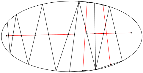
Let be a primitive closed geodesic of with positive geometric self-intersection number. Choose a representative in the free homotopy class of closed curves corresponding to , so that has only transverse self-intersections and minimal self-intersection number. We can also assume that only has simple self-intersection points, i.e. if we choose a parameterization of by , then implies that . Let be a point of self-intersection for .
There is a well-known procedure one can apply to known as surgery at to obtain new closed curves in . To do so, choose a small topological disc in so that is four points that lie along in that order, and is the union of two simple paths that intersect at , one with endpoints and , and the other with endpoints and . We can then modify the curve by replacing the two simple paths that intersect at with two simple paths in that do not intersect. There are two ways to do so; we can either replace with two simple, non-intersecting paths in with endpoints and , or we can replace with two simple, non-intersecting paths in with endpoints and .
These two different ways of performing surgery to at yield either one closed curve in or two closed curves and in . For , let correspond to the free homotopy class of closed curves in that contains (see Figure 2). It is easy to see that , and do not depend on the choice of . Moreover, an easy homotopy argument shows that , and also do not depend on in the following sense. If is another closed curve in the free homotopy class corresponding to with minimal geometric self-intersection number and only simple, transverse self-intersection points, then the homotopy between and gives a bijection
If we perform surgery to at the self-intersection point in both ways, then the closed geodesics corresponding to the free homotopy classes of closed curves we obtain are exactly , and .
The following proposition gives useful inequalities involving , , and .
Proposition 4.5.
Let and let be a primitive closed geodesic so that . By performing surgery to at a point of self-intersection in two different ways (see discussion above), we obtain either a single geodesic or a pair of geodesics , . Then
Furthermore, these inequalities are strict when has full support.
Proof.
Let be a group element so that . Choose a hyperbolic structure on , and let be a closed curve homotopic to with transverse, minimal self-intersection and only simple self-intersection points. The homotopy between and gives a surjection
Let be the self-intersection point of where the surgeries to obtain , and are performed, and let .
Let be the axis of , and observe that is a lift of the geodesic . Let be a point in whose image under the covering map is . Then also lies in and as well. Let be the group elements so that , , and (see Notation 4.2). It is clear that and .
We will first prove the inequality . By (2) of Lemma 4.4, we have
To prove the inequality , first make the following observation. For any , let be the geodesic in containing . If , then as well, so the -measure of the set of geodesics through that are transverse to , is equal to the -measure of the set of geodesics through , which is again equal to the -measure of the set of geodesics through transverse to . This is in turn equal to the -measure of the set of geodesics through transverse to . Hence, we may conclude that if , then
Now, observe that the geodesic containing is . Hence, the previous observation, together with (2) Lemma 4.4, allows us to conclude that if , then
With this, we can prove for general . Since is obtained from by performing surgery, it is clear that . Also, since is a lift of , we can write for some so that . This means that
Finally, we argue that these inequalities are strict when has full support. By the strictness statement in (2) of Lemma 4.4, it is sufficient to show that does not lie along the axes of , and . This is obvious, since the axes of , , and are pairwise disjoint. ∎
4.4. Asymptotics of lengths
In [5], Burger and Pozzetti consider a metric compactification of the space of -maximal representations. The limit points correspond to actions via isometries of on certain asymptotic cones. They prove (Theorem 1.1 of [5]) that a boundary point determines a decomposition of into essential subsurfaces. This decomposition is defined in terms of the asymptotic behavior of the length function.
In this section, we obtain an analogous result for sequences of positively ratioed representations as a consequence of Theorem 1.1. Here, we use the compactness of the space of projectivized geodesic currents (Corollary 5 of [2]) to describe the limit points. First, we need the following lemma.
Lemma 4.6.
Let and be a primitive non-simple curve. Then there is some geodesic pair of pants and so that
-
•
-
•
is primitive and has a unique self-intersection point
-
•
the three closed geodesics , and obtained by performing surgery to at in the two different ways specified in Section 4.3 are the three boundary components of .
-
•
if a curve intersects transversely, then intersects transversely.
Proof.
Let be any self intersection point of and let , and be the three closed geodesics obtained by performing surgery to at . It is clear that the self-intersection numbers of , and are less than that of . Also, Proposition 4.5 implies that for all . Suppose that there is some so that is not a multiple of a simple curve. Then let be the closed geodesic so that for some primitive with the property that for some . Then is primitive, non-simple, has fewer self-intersection points than , and . Replace with .
Iterate the replacement procedure above. This iteration will terminate to give a non-simple so that , and for any self-intersection point of , the three closed geodesics , and obtained by performing surgery to at are multiples of simple curves in . This then implies that must have a unique self-intersection point. In particular, , and are simple and are pairwise non-intersecting. The homotopy from , and to is a pair of pants that contains , and has , and as its boundary components. ∎
Proposition 4.7.
Fix an auxiliary hyperbolic structure on . Let be a sequence of non-zero geodesic currents. There is
-
•
a subsequence of , also denoted ,
-
•
a (possibly disconnected, possibly empty) essential subsurface ,
-
•
a (possibly empty) collection of pairwise non-intersecting, simple closed geodesics
so that is non-empty, and the following property holds. Let be a closed curve so that and is not a multiple of for .
-
(1)
If is a multiple of for some or , then .
-
(2)
If is a closed curve so that and is not a multiple of for , then .
Proof.
Since the weak∗ topology on is metrizable and is compact, there exist
-
•
a subsequence of , also denoted ,
-
•
a sequence of positive real numbers ,
-
•
a non-zero geodesic current ,
such that . Define
and consider .
For our choice of an auxiliary hyperbolic metric on , let be a maximal (possibly empty) collection of pairwise non-intersecting simple closed geodesics that do not have transverse intersections with any geodesic in . Then let be the list of connected components of and define
If , set to be . Otherwise, let be the closed geodesics in .
Notice that is non-empty because is non-empty. Since the intersection pairing is continuous, for any and for any intersecting transversely a geodesic in , up to passing to a further subsequence, we have
Also, if and only if intersects some geodesic in transversely. It is thus sufficient to show that for any , intersects a geodesic in transversely if and only if is not a multiple of for and .
Clearly, if is a multiple of for some or , then does not intersect any geodesic in transversely. To prove the converse, suppose that is not a multiple of for , and . If intersects transversely for some , we are done. Hence, for the rest of the proof, we will assume that intersects the interior of . The proof proceeds in two cases.
Case 1: Suppose . By the way is constructed, if is simple, then it must intersect a geodesic in (otherwise the maximality of is contradicted). Hence, we may assume that is non-simple. By Lemma 4.6, we may also assume that is contained in a geodesic pair of pants . Since is a non-peripheral geodesic in , it has transverse intersections with every non-peripheral geodesic in and every geodesic segment in with endpoints in . Also, because , there is some geodesic in that intersects the interior of . Hence, intersects some geodesic in transversely.
Case 2: Suppose is not entirely contained in . Let be a connected component of so that intersects the interior of , and let be the set of geodesics in that lie in . Let and be a pair of points where intersects the boundary of in , so that there is a subsegment of with endpoints and that is entirely contained in . Let and be the boundary components of containing and , respectively.
For , choose a parameterization so that and choose a parameterization so that and . Consider, the closed curve , where is the symbol for concatenation. Observe that is freely homotopic to a non-peripheral geodesic in . By the previous case, we know that intersects a geodesic in , so also intersects a geodesic in . Since and are boundary geodesics, they do not intersect any geodesics in . This means that intersects a geodesic in . Moreover, since is a geodesic segment, this intersection is transverse. Hence, intersects a geodesic in transversely in this case as well. ∎
4.5. Systoles and minimal pants decompositions
We will now explore the consequences of Proposition 4.5 on systole lengths of any essential subsurface . If is period minimizing, then the function given by is minimized at some . The same idea gives us a notion of systoles for essential subsurfaces, which we will now define.
Definition 4.8.
Let be an essential subsurface, and let be period minimizing. The -systole length of is
and a -systole of is a closed geodesic so that . Also, define the -interior systole length of to be
and a -interior systole of is a non-peripheral closed geodesic so that . In the case when , we will denote .
Using Proposition 4.5, we can prove the following corollary.
Corollary 4.9.
Let be a connected essential subsurface and let be period minimizing. Suppose that is not a pair of pants. Then the following hold.
-
(1)
There is a -interior systole of that is simple.
-
(2)
If has full support, then every -interior systole of is simple.
Proof.
Let be a -interior systole of . We may assume without loss of generality that is primitive. Suppose that has self-intersections. Then we can perform surgery to at some point of self-intersection to obtain , and with and . If , and are all peripheral, then the relation implies that is a pair of pants, which contradicts the hypothesis of the corollary. Hence, for some , is a non-peripheral closed geodesic whose self-intersection number is strictly less than the self-intersection number of .
Proof of (1). By Proposition 4.5, we know that is also a -interior systole of , so we can iterate the above procedure with in place of . This will eventually terminate after at most steps to give a -interior systole that is simple.
Proof of (2). In the case when has full support, Proposition 4.5 tells us that . This contradicts the fact that is a -interior systole. ∎
In particular, if we have a period minimizing , we can build a -minimal pants decomposition, denoted , on any essential subsurface . Let be the boundary components of . If is a disjoint union of pairs of pants, then is three times the number of components of and . Otherwise, Corollary 4.9 implies that there is a -interior systole of that is simple. Let be such a -interior systole of , then is again an essential subsurface of . Hence, we can iterate this procedure until we have a pants decomposition . Denote simply by .
5. Combinatorial description of
In this section, fix some that is period minimizing. An important ingredient in the proof of Theorem 1.4 is a finite combinatorial description, defined below, for each conjugacy class in that is adapted to . The methods in this section and the following one are inspired by work of the second author [37].
5.1. Minimal pants decompositions and related structures
First, we need to equip with an ideal triangulation which depends on and .
Definition 5.1.
An ideal triangulation of is a maximal -invariant subset such that the following hold:
-
(1)
Any two pairs of geodesics do not intersect transversely.
-
(2)
For any geodesic , one of the following must hold:
-
•
There is some in such that .
-
•
There is some such that is the set of fixed points of .
-
•
An ideal triangulation of is then the quotient for some ideal triangulation of of . A triangle is an unordered triple of geodesics in of the form .
If we choose a hyperbolic structure on , then every ideal triangulation of can be realized as an ideal triangulation of (in the classical sense) by assigning to each pair the unique hyperbolic geodesic in with endpoints . Moreover, this ideal triangulation is -invariant, so can be thought of as an ideal triangulation (in the classical sense) of .
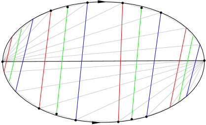
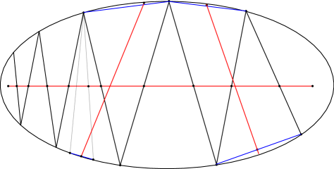
For our purposes, we will consider a particular ideal triangulation of , defined as follows. Choose an orientation on . Recall that we previously constructed a -minimal pants decomposition of as a consequence of Corollary 4.9. Extend this to a pants decomposition of , and let be the pairs of pants given by where is the genus of . For each , orient each component of so that lies on the left of the boundary component. Let be primitive group elements corresponding to the three boundary components of equipped with their orientations, so that . For each and , let denote the attracting and repelling fixed points of respectively.
Let and be the subsets of defined by
and note that both and do not depend on the choice of , and . They are also -invariant, so we can define and . With this, define
and observe that and are ideal triangulations of and respectively.
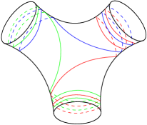
It is clear that (recall that sends to ). Also, if we choose a hyperbolic structure on , then for all , the three geodesics in correspond to three simple, pairwise non-intersecting geodesics in the hyperbolic pair of pants that each “spiral” towards two different boundary components of (see Figure 3).
The ideal triangulation by itself is insufficient to give a finite combinatorial description for the geodesics in . We need to make some additional choices, which we will now specify.
Choose
-
•
an orientation on each simple closed geodesic in .
-
•
a hyperbolic structure on .
Since we have chosen orientations on every , can be viewed as a conjugacy class in . For any such , let be a primitive group element so that . Then let
and define
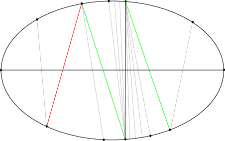
Observe that and are both invariant under the cyclic subgroup . Also, the geodesics in are realized as hyperbolic geodesics in , and their union bounds a simply connected, convex domain that contains the axis of . Let and be the two pairs of pants given by that have as a common boundary component, so that and lie on the left and right of respectively. (It is possible that ).
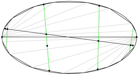
Choose a point on a hyperbolic geodesic in , and let be a point so that
Observe that this minimum exists because
Also, let be the points so that correspond to the hyperbolic geodesics in that contain (see Figure 4).
By reversing the labeling of and if necessary, we can assume without loss of generality that the hyperbolic geodesics corresponding to and do not intersect. Then define
and
Note that induces orderings on and . Also, for , , which consists of two geodesics in when and one geodesic in when .
5.2. Binodal edges and winding
Let be the conjugacy class of any non-identity element. We can now define (given all the choices made above) a finite combinatorial description for each conjugacy class , which is adapted to .
Recall that we have already chosen a hyperbolic structure on .
Definition 5.2.
Let be either a geodesic or geodesic subsegment. Also, for any , let be the axis of .
-
•
Let be the set of geodesics in that intersect transversely. A point in is a node of if it is the common endpoint of two distinct geodesics in . We call a geodesic in binodal if both of its endpoints in are nodes. Denote the set of binodal edges in by .
-
•
In the case when , observe that and are both -invariant, so we can define and .
Observe that we can think of and as cyclic sequences of geodesics in . In that case, they depend only on the conjugacy class of , and not on itself. Also, is finite, and is empty if and only if . For the rest of this section, we will assume that is non-empty unless stated otherwise.
The orientation on induces a natural ordering on . Also, since does not contain any of its accumulation points, we can define a bijective successor map . Moreover, the ordering induces a cyclic order on , and the successor map descends to a successor map .
The orientation on induces an orientation on . Let and be the two connected components of , oriented from to , so that the orientation on agrees with the orientation on .
Definition 5.3.
(See Figure 5.) Let be an edge in and assume without loss of generality that lies in and lies in . We say is
-
•
Z-type if and ,
-
•
S-type if and .
Let be the edges in that are Z-type and be the edges in that are S-type. Since and are -invariant, we can define and .
Again, and , when viewed as a sequence of geodesics in , depend only on the conjugacy class of . Also, note that , and the cyclic order on induces cyclic orders on , and . Let and be consecutive geodesics in so that precedes . Then the following must hold:
-
(1)
If and are not of the same type, then there are representatives of , respectively so that and share a common endpoint in , and .
-
(2)
If and are of the same type, then there are representatives of , respectively so that there is a geodesic in that has a common endpoint with each of and , and .
If (1) holds, let be the primitive group element that has the common vertex of and as a fixed point, and so that the conjugacy class corresponds to an oriented closed geodesic in . On the other hand, if (2) holds, let be the element in whose axis is the geodesic in that has common endpoints with and , and so that the conjugacy class corresponds to an oriented closed geodesic in . If , the closed geodesic in corresponding to is in .
Notation 5.4.
For , let be the signed number of edges in that intersect . Here, the sign is positive if the orderings on these edges induced by and by agree, and is negative otherwise.
The quantities for do not depend on the choice of and . Also, they do not depend on the choice of in the following sense: if for some , then and are consecutive elements in , and .
Notation 5.5.
Let be a geodesic segment that intersects the geodesics in transversely. For , let denote the number of edges in that intersect respectively.
It is clear that , and that .
Cyclically enumerate , and for each , let be the type (Z or S) of . Then define the cyclic sequence of tuples
This is the combinatorial description of mentioned at the start of the section.

Let be the collection of cyclic sequences of the form , where are the three distinct edges in for some , is the symbol S or Z, and . For any term of the sequence , let
Also, let and be lifts of and respectively that share a common endpoint in , and let be the group element whose repelling fixed point is this common endpoint. Then there are exactly two geodesics and in with lifts and in respectively that have as a common endpoint. Let be the edge in so that for some (see Figure 6).
Definition 5.6.
We say a sequence in is admissible if for all , is one of the following:
(Notice that the last two cases correspond to crossing the pants curve .) Let denote the set of admissible sequences in .
Observe that can be viewed as a map from to . The most important property of is its injectivity, which was previously proven by the second author (Proposition 4.5 of [37]).
Proposition 5.7.
Let be elements in . Then if and only if .
Notation 5.8.
-
•
For any cyclic sequence , let and let .
-
•
If , let
and for , let
Note that , , and are well-defined as they do not depend on the orientation on induced by . Also, note that and . Informally, is the number of times cuts across pants curves, is the number of times crosses a binodal edge in , and and are two different ways of measuring how many times “winds around” collar neighborhoods of the curves in .
The advantage of over is that can be read off the combinatorial description . On the other hand, we will later obtain a lower bound for in terms of . In the following lemma, we make the relationship between and explicit.
Lemma 5.9.
Let and let . Then
Proof.
First, observe that for any consecutive pair with preceding , we have
Summing the above inequality over all consecutive pairs in yields the required inequality. ∎
6. Lengths and geodesic currents
In this section, we will prove some inequalities about lengths of closed geodesics which depend on their intersections with a -minimal pants decomposition and the corresponding ideal triangulation as defined in Section 5. For the rest of this section, fix a period minimizing geodesic current , a hyperbolic structure on , and an essential subsurface of . The goal of this section is to prove Theorem 6.8. For any , this theorem gives a lower bound of in terms of the -panted systole length, the -systole length, and the combinatorial description and defined in Section 5.
6.1. Length lower bounds: intersection with pants curves
We begin by first finding a lower bound for in terms of the number of times intersects . To do so, we define the following quantity.
Definition 6.1.
Let be a -minimal pants decomposition of . Define the -panted systole length to be
Lemma 6.2.
The -panted systole length does not depend on the choice of a minimal pants decomposition . Namely,
for any minimal pants decomposition .
Proof.
Assume there exists a minimal pants decomposition such that
is greater or equal to . We claim that this implies . Let so that is not a multiple of a geodesic in , and . The minimality of implies that is primitive.
If is not a simple closed geodesic in , then we are done because
On the other hand, if , then the fact that is simple implies that there are closed geodesics so that . Let be such a closed geodesic so that is minimal, and observe that by the definition of a -minimal pants decomposition. Also, since , we have , so . Therefore,
One finishes the proof by reversing the roles of and if . ∎
With the notion of a panted systole length, we have the following lemma.
Lemma 6.3.
Let be a simple -interior systole of , and let be points such that the interval intersects transversely. Then
where is the set of geodesics defined in Notation 4.3.
Proof.
First, observe that since is compact, is finite. Also, if or , then the desired inequality clearly holds. Thus, we will assume for the rest of this proof that . Let be the points in in that order along , where . For any , let denote a group element so that
-
•
,
-
•
the axis of contains .
The proof will proceed in two cases from here.

Case 1: . Then for , let be a group element so that
-
•
,
-
•
,
and let be the closed geodesic such that (see Figure 7). Note that is not a multiple of a curve in because it has positive geometric intersection number with , so . By (1) of Lemma 4.4, we have for all . The definition of implies that
for all . Then by (2) of Lemma 4.4, we have that
Case 2: . Let be a -minimal pants decomposition of that contains . For any , let and let be the closed geodesic such that . Note that is not a multiple of a curve in because and has positive geometric self-intersection number, so . Thus, by Lemma 4.4,
As a consequence of the above lemma, we obtain the following corollary.
Corollary 6.4.
Let be a simple -interior systole of . For any ,
Proof.
If or , the corollary clearly holds. For the rest of this proof, we will assume that . Choose a hyperbolic structure on . Then and are realized as closed geodesics in . Choose a point and a point so that . Let be a group element so that and lies in the axis of . Then . Hence, by (1) of Lemma 4.4 and Lemma 6.3, we have
By applying Lemma 6.3 to all the curves in a -minimal pants decomposition on , we can also obtain the following lower bound on in terms of the number of times intersects the curves in a -minimal pants decomposition .
Lemma 6.5.
Suppose that is a connected essential subsurface of genus with boundary components. Let so that the boundary components of are , and let . Then
Proof.
Assume without loss of generality that for all . If
(this has to happen when is a pair of pants), the desired inequality holds, so we assume that in the rest of this proof.
Let so that and let so that
Then let and let be the points in
enumerated so that for all . Observe that .
We will now show that for all . If the interval intersects at least thrice, then Lemma 6.3 implies that
and we are done. (This is necessarily the case if .) On the other hand, if intersects at most twice, then by the pigeon hole principle, there is some so that does not intersect . In other words, there is a component of so that the interval lies in some lift of the subsurface . Since , it follows that cannot be a pair of pants.
If intersects at least thrice, then Lemma 6.3 again implies that
(This is necessarily the case if .) Otherwise, intersects at most twice, so there must be some with the property that does not intersect . Hence, there is a component of so that lies in some lift of the subsurface . As before, cannot be a pair of pants because .
By iterating this procedure, times, we will have either already proven that , or have some and some component of so that
-
•
is not a pair of pants
-
•
lies in some lift of the subsurface .
In this case, the unique simple closed geodesic in is , and necessarily intersects at
Lemma 6.3 then implies that
6.2. Length lower bounds: winding and intersection with binodal edges
In this section, fix a -minimal pants decomposition . Next, we want a lower bound of in terms of and . To do so, we need the following two technical lemmas. Informally, Lemma 6.6 tells us how much length has to pick up if it crosses sufficiently many binodal edges. On the other hand, Lemma 6.7 tells us how much length has to pick up if it “winds around” a lot between binodal edges.
Lemma 6.6.
Let be a pair of pants given by and let be the universal cover of . Also, let be points so that intersects the geodesics in transversely (if at all). Then
(See Definition 5.2 for definition of .)
Proof.
If , the desired inequality holds, so we will assume for the rest of this proof that . Let be the points along that also lie in the geodesics in , enumerated so that they lie along in that order. Suppose that for all , we have . Then
It is thus sufficient to show that for all . Fix any . For all , let and let be the geodesic in that contains . Observe that and share a common endpoint in , which is the repelling fixed point of some primitive so that is a boundary component of . Denote this common endpoint by . We will first prove the following claim: there exist so that and
This will be done in the following cases.
Case 1: There is some so that and for . In this case, let . By replacing with if necessary, we can assume that . Observe that is an edge in that forms a triangle with and . On the other hand, is an edge in whose endpoints in both lie in (see Notation 2.26). Thus, is non-empty (see Figure 8).
Case 2: There is a unique so that . In this case, let , let if and let if . The same argument as Case 1 will show that is non-empty. We will now prove that is non-empty when ; the case when is similar. By replacing by if necessary, we can assume that . Observe then that , , and (see Figure 9). In particular, is non-empty.
Case 3: For all , . In this case, let and let . The argument given in Case 2 proves that is non-empty for . This concludes the proof of the claim.
Next, we will use the claim to prove the lemma. Assume without loss of generality that . Let be points so that . (They exist because of the claim.) By replacing each with if necessary, we can assume that lie along in that order. Observe then that has to lie in , has to lie in , has to lie in and has to lie in . In particular, lie along in that order, and . It is clear that is non-peripheral. Hence, Lemma 4.4 implies that
Lemma 6.7.
Proof.
Let and note that if there is nothing to prove. Therefore, assume and let be the points in
in that order along . Fix any , let and assume without loss of generality that . Also, assume that lie along in that order; the other case is similar. Then
where the first inequality above is a consequence of the way and are defined.
6.3. Length lower bounds: the combinatorial description
Combining the previous lemmas in this section, we can obtain the following lower bound for in terms of the -panted systole length and the -systole length.
Theorem 6.8.
Let be a connected essential subsurface of genus with boundary components, let
Then
Proof.
By Lemma 6.5, we know that
| (6.1) |
Let so that , let so that
(recall , where are the boundary components of ) and let be the points in
enumerated so that for all .
Note that for any pair of pants given by , . Hence, by Lemma 6.6, we have
Adding the inequalities (6.1) and (6.3) then gives
| (6.3) |
Let . For each interval , let be the edges in , enumerated so that for all , where . We previously observed (see discussion after Notation 5.4) that the interval lies in . Also, it is clear that for every point , there are at most four different values of so that . Thus, by Lemma 6.7,
We finish the proof by combining the above inequalities to obtain a positive lower bound for . To ensure positivity of this lower bound, we need to add the above inequality to a multiple (strictly greater than 16) of inequality (6.3). We choose this multiple to be 20 to improve readability.
where the third inequality follows from Lemma 5.9. Dividing both sides by yields the required inequality. ∎
7. Vanishing of entropy and a systolic inequality
For the rest of this section, let be a connected essential subsurface of genus with boundary components. If we choose a period minimizing , we can associate to a quantity which we call the topological entropy.
Definition 7.1.
Let be a period minimizing geodesic current. The -topological entropy of is
When , we will use the notation .
7.1. A systolic inequality
The goal of this section is to prove Theorem 1.4. The constant that arises from our proof is . We will divide the proof of Theorem 1.4 into three lemmas. The first two lemmas give us the first inequality.
Lemma 7.2.
Let be a period minimizing geodesic current and be a -minimal pants decompositions of . Then there exists a pair of pants and a closed geodesic so that
-
•
has a unique self-intersection point ,
-
•
,
-
•
the three closed geodesics obtained by performing surgery to at are the three boundary components of .
Proof.
By Lemma 4.6, it is sufficient to construct a primitive, non-simple so that .
Let be a closed geodesic that is not a multiple of a curve in , and so that . Note that is primitive. If is non-simple, set to be and we are done. If is simple, then there is some that intersects transversely, so that . Choose a hyperbolic structure on . There exists so that , , and the axes and of and respectively intersect transversely. Let be the intersection point of and .
Lemma 7.3.
Let be a period minimizing geodesic current. Then
Proof.
Let , , and be as in Lemma 7.2. Let be primitive elements so that , and so that the closed geodesics , , are the boundary components of . Then has to be either
Assume without loss of generality that . Then
so and . Since is a free group of rank 2 generated by and , no two distinct elements of the form
are conjugate, where .
Now, we finish the proof of Theorem 1.4 by proving the second inequality.
Lemma 7.4.
There is a constant which depends only on the topology of , so that for any period minimizing , we have
where is the unique positive solution to the equation .
Proof.
Simplify notation by denoting and defined in the statement of Theorem 6.8 simply by and respectively. Choose a -minimal pants decomposition . By Theorem 6.8 and Proposition 5.7, we have
(See Definition 5.6 for the definition of .)
If , let be the cyclic sequence
For any , let be the geodesics so that for some . If , then there are four possibilities for , namely
Since , we see from the definition of that
Hence,
which implies that for ,
where is the integer so that for all ,
7.2. Corollaries of the systolic inequality
Theorem 1.4 has several interesting corollaries, which we will now explain. The first is a slight simplification of the inequality in Theorem 1.4 from which we can deduce all our other corollaries.
Corollary 7.5.
There is a constant which depends only on the topology of , so that for any period minimizing , we have
Proof.
Let , and consider the function defined by . Observe that is increasing, , and . Also, let be the unique point in so that . It is sufficient to show that for all ,
First, consider the case when . Then and . We see immediately that in this case, the required inequality holds.
Next, consider the case when . The equation can be rearranged as
Since the function given by is positive and strictly decreasing, we see that is minimized over all when is maximized. From the definition of , it is clear that is strictly decreasing with , so is minimized over all when . It is easy to compute that , so for all . Hence,
Using Corollary 7.5, we have the following universal upper bound on the systole length renormalized by the entropy.
Corollary 7.6.
There is a constant which depends only on the topology of , so that for any period minimizing , we have
Proof.
By Corollary 7.5, we see that there is a constant depending only on the topology of , so that for any period minimizing ,
where the last inequality holds because for all and . ∎
Corollary 7.6 together with Theorem 1.1 proves Corollary 1.5. Also, given any negatively curved Riemannian metric on with geodesic boundary, one can always find a negatively curved Riemannian metric on whose restriction to is . It is then known (see Proposition 3 of Otal [29]) that the Lebesgue-Liouville current of has the property that , where is the length function induced by . This fact combined with Corollary 7.6 then gives us Corollary 1.6.
Corollary 7.5 also gives us a criterion that determines when the topological entropy of a sequence of geodesic currents in the “-thick” part of converges to . Before we state the corollary, we first define what the “-thick” part of is.
Definition 7.7.
Let be the set of period minimizing geodesic currents and let . Define
and .
Observe that if lie in the same equivalence class in , then . Thus, we can think of as a function from to .
Corollary 7.8.
Let be any positive number and let be a sequence in . Then if and only if the following condition holds: for each , there is a (possibly empty) collection of pairwise non-intersecting simple closed geodesics in so that
-
•
, and
-
•
Proof.
Let us choose an appropriate collection of closed geodesics. For each , let be a minimal pants decomposition, where are non-peripheral and enumerated so that . Let be the number so that
-
•
for all ,
-
•
for all .
(We use the convention if and if .) Let
First, we show that if the condition does not hold, then . Since the condition does not hold, there is a constant so that for each , there is a component of and a non-peripheral primitive closed geodesic satisfying . Notice that when , is a pair of pants which implies that is primitive and non-simple. Likewise, if , for sufficiently large , is primitive and non-simple because for all . In either case, for all . Thus, by Corollary 7.5. Since , we see that .
Next, we suppose that the condition holds and we prove that . Observe that for big enough, the curves in are part of a minimal pants decomposition . Let be a closed geodesic that is not a multiple of an element in so that . By Corollary 7.5, it is sufficient to show that . Choose a hyperbolic structure on , set , and set . Since the condition holds, and .
If , then it is non-peripheral, so
On the other hand, if does not lie in , let be a component of that intersects . Let be the group element so that and let be the axis of in . Choose distinct points so that and for all . It is clear that
Let be the group elements so that , and and lie in the axes of and respectively. Observe that . Hence, by Lemma 4.4,
Similarly, . Since cannot both be peripheral, either or . Thus,
This implies that . ∎
Appendix A From positive cross ratios to geodesic currents
In this appendix, we give a proof Theorem 2.10 (which was previously observed by Hamenstädt [15]) for the convenience of the reader. Recall that an algebra on a set is a family of subsets of so that
-
(1)
for all in , the complement of is in ,
-
(2)
for all , the union .
Also, a premeasure on is a function
such that
-
(1)
;
-
(2)
if is a countable family of pairwise disjoint sets in whose union lies in , then
Choose an orientation on . For the rest of this appendix, we will assume that all intervals in are of the form (see Notation 2.26) unless otherwise stated, where lie in in the order specified by the orientation. We will start by defining a particular algebra in .
Definition A.1.
Let be a finite list of pairs of proper subintervals of .
-
•
is an admissible list if for all , either or and are disjoint.
-
•
For any admissible list , let denote the set of geodesics such that there exists a with and each containing one endpoint of .
For the rest of this appendix, let . Note that every can be written as a finite disjoint union
Lemma A.2.
is an algebra.
Proof.
For all , note that . To prove closure under complements, it is sufficient to show that and because of De Morgan’s laws.
First, we will show that . If and have disjoint interiors, let be the endpoints of and be the endpoints of . Also, let and , and observe that is a disjoint union. It is then easy to see that , where
On the other hand, if , let . Then , where .
Next, we will show that . Let be intervals so that is a disjoint union. (Note that is either , or .) Then observe that , where
∎
Next, we will use the positive cross ratio to define a premeasure on . Let be a function defined as follows:
-
(1)
.
-
(2)
when or and share a common endpoint.
-
(3)
If the intervals and are non-empty and have disjoint closures, let and be the endpoints of and and the endpoints of , so that , , , lie in this cyclic order along . Then define
-
(4)
If is a disjoint union, define
Since , is well-defined. Also, if
are two ways to write as disjoint unions, then by taking intersections, we can write as the disjoint union
so that for all , is a connected component of for some and . By the additive property of the cross ratio, if are subintervals of so that , then This implies that
so is well-defined.
It is also clear from the definition that is finitely additive, i.e. if are pairwise disjoint, then
Furthermore, the positivity of , ensures that takes values in .
Proposition A.3.
For any positive cross ratio , is a premeasure on .
Proof.
Set to simplify the notation. By definition, , so we need only to prove countable additivity. Let be a family of disjoint sets in with for some admissible list . Up to repartitioning and renumbering, we can assume the following:
-
•
For all , for some intervals ,
-
•
There is some admissible list so that is a disjoint union.
By finite additivity, we have that for all ,
Thus, .
To finish the proof, we need to show that . First consider the case where , then for all , . Since is continuous, for any and any , we can find compact subintervals and such that
| (A.1) |
Similarly, for any we can find open intervals and such that
| (A.2) |
Observe that the open sets is an open cover of the compact set , so it has a finite subcover . By using inequalities (A.1) and (A.2), we have
Since was arbitrary, this proves that when .
Next, consider the case where . This means that for some , so either and are disjoint and share an endpoint, or . In either case, we can find subintervals and that are disjoint and share an endpoint. Let be the common endpoint of and , let be the endpoint of that is not , and for any let be the subinterval of with endpoints and . Since
we know that for every , there exists in the interior of such that . Using the previous case, we know that for all ,
Thus, . ∎
We will now recall a standard procedure to obtain a unique measure extending a premeasure. See for example Chapter 1 of Folland [9] for more details. Given a premeasure on and , define the outer measure
A premeasure is -finite if can be written as a union of countably many sets with finite outer measure. The following theorem (Theorem 1.14 of [9]) relates -finite premeasures and measures.
Theorem A.4.
Let be the -algebra generated by . Then, is a measure on and the restriction of to is . If is -finite, then is unique.
Lemma A.5.
If is a positive cross ratio, then the premeasure is -finite.
Proof.
Let be a countable dense subset of . For any and , let be the open interval in centered at of width . Define
Clearly
| (A.3) |
Observe that the right hand side of Equation A.3 is a countable union of sets, each with finite measure. ∎
Proof of Theorem 2.10.
Since the premeasure is -finite, Theorem A.4 ensures that there is a unique measure on the -algebra generated by . The -invariance of ensures that is also -invariant. It is easy to see that the topology on lies in . Thus, is a geodesic current.
Next, we show that for all , . By (1) of Lemma 4.4, we know that
Appendix B Computation for proof of Theorem 1.4
The goal of this appendix is to prove the following statement, which we need to finish the proof of Theorem 1.4.
Proposition B.1.
Let be positive numbers so that . Also, let be an integer so that for all , we have
Then
where is the unique positive solution to the equation .
The proof of Proposition B.1 is a refinement of the argument given in Appendix B of [36]. However, we will make this appendix self-contained for the convenience of the reader. The main tool in this computation is an old result known as Stirling’s formula, which we state here.
Theorem B.2 (Stirling’s Formula).
.
In order to use Stirling’s formula, we need to prove the following lemma. For the rest of this appendix, let
Lemma B.3.
Let be fixed numbers, and . Then the following hold:
-
(1)
.
-
(2)
.
-
(3)
.
-
(4)
.
Proof.
From the definition of , we see that
| (B.1) |
which can be rearranged to be
| (B.2) |
Similarly, the definition of also tells us that
| (B.3) |
which implies
| (B.4) |
Proof of (1). Suppose for contradiction that . By the definition of , we see that . Thus,
which contradicts (B.4).
Proof of (2). Suppose again for contradiction that . By taking an appropriate subsequence, we can assume that . Hence, , so we have
On the other hand, if and , then the right hand side of the inequality (B.2) converges to as , which implies that
This is a contradiction.
Proof of (3). Since (1) and (2) hold, taking the limit infimum of (B) as gives
Proof of (4). Similarly, by taking limit supremum of (B) as , we get
By (3) and (4) of Lemma B.3, we see that is a positive real number, which we will denote by in the sequel. We now use (3) of Lemma B.3 to find an inequality relating to .
Lemma B.4.
For any positive numbers , let . Then
where is the unique positive solution to the equation .
Proof.
Consider the function defined by , and observe that is increasing, , and . By (3) of Lemma B.3, we know that , so . ∎
References
- [1] F. Bonahon, Bouts des variétés hyperboliques de dimension 2, Ann. Math. 124 (1986), 71-158.
- [2] F. Bonahon, The geometry of Teichmüller space via geodesic currents, Invent. Math. 92 (1988), 139-162
- [3] M. Burger, A. Iozzi, F. Labourie, A. Wienhard Maximal representations of surface groups: Symplectic Anosov structures, Pure Appl. Math. Q. 1 (2005), Special Issue: In memory of Armand Borel, 543-590.
- [4] M. Burger, A. Iozzi, A. Wienhard Surface group representations with maximal Toledo invariant, Ann. of Math. 172 (2010), 517-566.
- [5] M. Burger, M. Pozzetti Maximal representations, non Archimedean Siegel spaces, and buildings, arXiv:1509.01184.
- [6] J. L. Clerc, B. Ørsted The Gromov norm of the Kaehler class and the Maslov index, Asian J. Math. 7 (2003), no. 2, 269-295.
- [7] A. Dominic, D. Toledo The Gromov norm of the Kähler class of symmetric domains, Math. Ann. 276 (1987), no. 3, 425-432.
- [8] P. Eberlein Geometry of nonpositively curved manifolds, Chicago Lectures in Math., Univ. of Chicago Press (1996).
- [9] G.B. Folland Real analysis, Pure and Applied Mathematics (New York) (1999).
- [10] F. Guéritaud, O. Guichard, F. Kassel, A. Wienhard Anosov representations and proper actions, to appear in Geometry and Topology, Preprint arXiv:1502.03811.
- [11] O. Guichard Composantes de Hitchin et représentations hyperconvexes de groupes de surface, J. Diff. Geom. 80 (2008), 391-431.
- [12] O. Guichard, A. Wienhard Anosov representations: domains of discontinuity and applications, Invent. Math. 190 (2012), 357-438.
- [13] W. M. Goldman Topological components of spaces of representations, Invent. Math. 93 (1988), no. 3, 557-607.
- [14] U. Hamenstädt, Cocycles, Hausdorff measures and cross ratios, Ergod. Th. & Dynam. Sys. 17 (1997), 1061-1081.
- [15] U. Hamenstädt, Cocycles, symplectic structures and intersection, Geom. Funct. Anal. (1999), Volume 9, 90 - 140.
- [16] S. Helgason Differential Geometry, Lie groups and Symmetric Spaces, Graduate Studies in Mathematics, Volume 34, American Mathematical Society (1978).
- [17] N. J. Hitchin Lie groups and Teichmüller space, Topology 31 (1992), no. 3, 449-473.
- [18] J. Humphreys Introduction to Lie Algebras and Representation Theory, Graduate Texts in Mathematics, Volume 9, Springer (1972).
- [19] M. Kapovich, B. Leeb, J. Porti Morse actions of discrete groups on symmetric space, Preprint arXiv:1403.7671.
- [20] M. Kapovich, B. Leeb, J. Porti A Morse Lemma for quasigeodesics in symmetric spaces and euclidean buildings, Preprint arXiv:1411.4176.
- [21] F. Labourie, Anosov flows, surface groups and curves in projective space, Invent. Math. 165 (2006), 51-114.
- [22] F. Labourie. Cross ratios, surface groups, and diffeomorphisms of the circle, Publ. Math. Inst. Hautes Études Sci. No.106 (2007), 139-213.
- [23] F. Labourie Cross Ratios, Anosov representations and the Energy Functional on Teichmüller space, Ann. Sci. École Norm. Sup. 41 (2008), Issue 3, (439-471).
- [24] F. Ledrappier Structure au bord des variétés à courbure négative, Séminaire de théorie spectrale et géométrie de Grenoble, 71, (1994-1995), 97-122
- [25] J. Milnor On the existence of a connection with curvature zero, Comm. Math. Helv. 32 (1958), 215-223.
- [26] X. Nie Entropy degeneration of convex projective surfaces, Conformal Geometry and Dynamics. 19 (2015), 318-322.
- [27] X. Nie On the Hilbert geometry of simplicial Tits sets, Annales de l’Institut Fourier 65 (2014), 1005-1030.
- [28] J-P. Otal Sur la géométrie symplectique de l’espace des géodésiques d’une variété à courbure négative, Rev. Math. Iberoam. 8 (1992), 441-456.
- [29] J-P. Otal Le spectre marqué des longueurs des surfaces à courbure négative, Ann. Math. 131 (1990), 151-162.
- [30] J.F. Quint Mesures de Patterson-Sullivan en rang supérieur, Geom. Funct. Anal. 12 (2002), 776-809.
- [31] A. Sambarino Quantitative properties of convex representations, Comm. Math. Helv. 89 (2014), 443-488.
- [32] A. Sambarino Hyperconvex representations and exponential growth, Ergod. Th. & Dynam. Sys. 34 (2014), no. 3, 986-1010.
- [33] S. Sabourau Entropy and systoles on surfaces, Ergod. Th. & Dynam. Sys. 26 (2006), no. 5, 1653-1669.
- [34] J. Tits Représentations linéaires irréductibles d’un group réductif sur un corp quelconque, J. Reine Angew. Math. 247 (1971), 196-220.
- [35] V. Turaev A cocycle for the symplectic first Chern class and the Maslov index, Funct. Anal. Appl. 18 (1984), 35-39.
- [36] T. Zhang, The degeneration of convex structures on surfaces, Proc. London Math. Soc. (2015), Volume 111, 967-1012.
- [37] T. Zhang, Degeneration of Hitchin representations along internal sequences, Geom. Funct. Anal. (2015), Volume 25, 1588-1645.