Integral estimation based on Markovian design

Abstract

Suppose that a mobile sensor describes a Markovian trajectory in the ambient space. At each time the sensor measures an attribute of interest, e.g., the temperature. Using only the location history of the sensor and the associated measurements, the aim is to estimate the average value of the attribute over the space. In contrast to classical probabilistic integration methods, e.g., Monte Carlo, the proposed approach does not require any knowledge on the distribution of the sensor trajectory. Probabilistic bounds on the convergence rates of the estimator are established. These rates are better than the traditional “root $n$”-rate, where $n$ is the sample size, attached to other probabilistic integration methods. For finite sample sizes, the good behaviour of the procedure is demonstrated through simulations and an application to the evaluation of the average temperature of oceans is considered.

Key-words: Integral approximation; Markov chains; Nummelin splitting technique; invariant density estimation; kernel smoothing.

1 Introduction

For the last decades, climate scientists have been interested in the evolution of different physical attributes of Earth to quantify the effects of global warming. For instance, attributes such as temperature, acidity and salinity of oceans or the concentration of greenhouse gases in the atmosphere are important indicators of global warming. Scientists measurements are often provided by sensors placed on drifting buoys in the oceans or weather balloons in the atmosphere, each describing an area or a volume. Whenever the data have been collected, a crucial quantity is the average of the measurements over a given space. As the sensors are eventually subjected to unpredictable effects such as marine currents or winds, their trajectories are modelled as random sequences. The approach taken here is concerned with trajectories satisfying the Markov property, meaning roughly that the distribution of the location at time $t+1$ is fully determined by the location at $t$ and an independent random noise. For the sake of realism, the underlying transition probability and the invariant probability measure associated to the Markov chain are supposed unknown. In summary, the aim is to evaluate the average value of a physical quantity over some space when the measurements are taken along the path of a Markov chain.

More formally, let $Q$ denote a given bounded and open set of $\mathbb{R}^{d}$ and suppose that $\varphi:Q\rightarrow\mathbb{R}$ represents a physical attribute to each location in $Q$, e.g., the temperature in the air over a volume or the wind velocity on the sea over a surface. For simplicity, the Lebesgue measure of $Q$ is set to be $1$. Hence, we are interested in the average value of $\varphi$ over $Q$, defined as

$$I_{0}=\int_{Q}\varphi(x)dx.$$

In most examples of interest the function $\varphi$ is unknown and only some images of the function are obtained from measurement instruments. Suppose that we observe $n\in\mathbb{N}^{*}$ points from the trajectory of a time-homogeneous Harris recurrent Markov chain $X_{1},X_{2},\ldots$ (Meyn and Tweedie, 2009) with state space $\mathcal{E}\supseteq Q$. Suppose moreover that we know the associated images by the map $\varphi$, i.e., $\varphi(X_{1}),\ldots\varphi(X_{n})$. Let $\pi$ denote the density of the stationary measure of the chain. If $\pi$ were known, it would be tempting to compute the Monte Carlo estimator of $I_{0}$,

$$\widehat{I}_{\text{mc}}=n^{-1}\sum_{i=1}^{n}\frac{\varphi(X_{i})}{\pi(X_{i})},$$

which satisfies, under standard conditions (Meyn and Tweedie, 2009, chapter 17), a central limit theorem, i.e., $n^{1/2}(\widehat{I}_{\text{mc}}-I_{0})$ converges weakly to a centered Gaussian distribution. As the previous estimator requires the knowledge of $\pi$, which is not the case in our framework, we rather consider the following kernel smoothing estimator of $I_{0}$,

$$\widehat{I}_{\text{ks}}=n^{-1}\sum_{i=1}^{n}\frac{\varphi(X_{i})}{\widehat{\pi}(X_{i})},$$

where $\widehat{\pi}$ is the classical kernel estimator of the density (Silverman, 1986), given by,

$$\widehat{\pi}(x)=(nh_{n}^{d})^{-1}\sum_{i=1}^{n}K((x-X_{i})/h_{n}),\qquad x\in\mathbb{R}^{d},$$

with $K:\mathbb{R}^{d}\rightarrow\mathbb{R}$, a symmetric function, called kernel, that integrates to $1$, and $(h_{n})_{n\in\mathbb{N}^{*}}$, a sequence of positive numbers, called bandwidth, that goes to $0$ as $n\rightarrow+\infty$.

As the stationary measure is unknown, we can not rely on Monte Carlo integration techniques, often used in simulation-based approximation, such as importance sampling, control variates or Metropolis-Hasting integration. We refer the reader to the books Evans and Swartz (2000) and Robert and Casella (2004) on integral approximation techniques.

The estimator $\widehat{I}_{\text{ks}}$ has been introduced in Delyon and Portier (2016) where the authors established bounds on the rate of convergence, in probability, in the case of independent and identically distributed sequence $X_{1},X_{2},\ldots$ Their main observation is that the convergence rate of $\widehat{I}_{\text{ks}}$ to $I_{0}$ is faster than the convergence rate of the Monte Carlo estimator $\widehat{I}_{\text{mc}}$ to $I_{0}$ (even though $\widehat{I}_{\text{mc}}$ requires the knowledge of $\pi$). In contrast to standard Monte Carlo methods, the main ingredient of their proposal is the evaluation of the image of the design points by the kernel estimator, i.e., $\widehat{\pi}(X_{1}),\ldots\widehat{\pi}(X_{n})$. These quantities capture an essential information : the isolation of each point. Basically, the more isolated $X_{i}$, the larger the weight $1/\widehat{\pi}(X_{i})$ (and conversely). Hence these weights realize an adaptation to the design points by attributing more weight to the lonely points. Such a strategy takes

The main theoretical objective of the paper is to extend the results of Delyon and Portier (2016) when the sequence $(X_{i})_{i\in\mathbb{N}^{*}}$ is a time-homogeneous Harris recurrent Markov chain. Denote by $s$ and $r$ the (Nikolski) regularity of the functions $\varphi$ and $\pi$, respectively. For any set $B\subset\mathcal{E}$, let $\tau_{B}$ denote the return-time of the chain to $B$. If there exists $A\subset\mathcal{E}$ and $p_{0}>3$ such that

$$\sup_{x\in A}\mathbb{E}_{x}[\tau_{A}^{p_{0}}]<+\infty,$$ (1)

where $\mathbb{E}_{x}$ is the expectation for the Markov chain starting at $X_{0}=x$, and if, as $n\rightarrow+\infty$,

$$\frac{nh_{n}^{d(p_{0}/p_{0}-1)}}{|\log(n)|}\rightarrow+\infty,$$

we show (Theorem 8), under mild additional conditions, that, as $n\rightarrow+\infty$,

$$\widehat{I}_{\text{ks}}-I_{0}=O_{\mathbb{P}}\left(h^{r}_{n}+n^{-1/2}h_{n}^{s}+n^{-1}h_{n}^{-d}\right).$$

This is the same convergence rate as the one provided in Delyon and Portier (2016) for independent and identically distributed sequences $(X_{i})_{i\in\mathbb{N}^{*}}$. The previous rate is better than the rate of $\widehat{I}_{\text{mc}}$ whenever $n^{1/2}h_{n}^{r}\rightarrow 0$ and $n^{-1/2}h_{n}^{-d}\rightarrow 0$, as $n\rightarrow+\infty$. Taking $h_{n}\propto n^{-1/(r+d)}$, we obtain a rate in $n^{-r/(r+d)}+n^{-1/2}n^{-s/(r+d)}$ which is negligible before $n^{-1/2}$ if and only if $r>d$. Consequently, in addition of being consistent when facing Markovian design, the kernel smoothing integral estimator might give an acceleration of the rate of convergence of the Monte Carlo estimator. This acceleration is unfortunately subjected to the well-known curse of the dimension as one needs that $r>d$. In contrast, a nice feature of the method is that only mild constraints are on the regularity of $\varphi$. Finally, there exists a theoretical lower bound for random integration methods (Novak, 2016, Theorem 3) which takes the following form $n^{-1/2}n^{-s/d}$ while our proposal achieves $n^{-1/2}n^{-s/2(s+d)}\geqslant n^{-1}$. This gap in efficiency might be explained by the design distribution which is imposed in our framework.

The mathematical proofs follow from a mixture between the Nummelin splitting technique for Markov chains (Nummelin, 1978), Hoeffding-type decompositions for $U$-statistics (van der Vaart, 1998, section 11.4) and uniform bounds for kernel density estimators in the case of independent observations (Einmahl and Mason, 2005). More specifically, the Nummelin splitting technique, also called regeneration theory and presented in section 2, allows for dividing the chain into $l_{n}$ independent blocks. Assumption (1) implies that $l_{n}$ and $n$ have the same order allowing us to mimic the approach of Delyon and Portier (2016) taken in the independent case:

1. Linearise the terms $1/\widehat{\pi}(X_{1}),\ldots 1/\widehat{\pi}(X_{n})$ by the help of a Taylor expansion. This is typically used in semi-parametric problems as for instance the single-index model (Härdle and Stoker, 1989; Vial, 2003).

2. Find a probabilistic bound on some degenerate $U$-statistic depending on the sequence $K((X_{j}-X_{i})/h)/h^{d}$, $(i,j)\in\{1,\ldots n\}^{2}$. We shall follow Bertail and Clémençon (2011) by using an Hoeffding-type decomposition based on the blocks.

3. Too small values of the denominator in $\widehat{I}_{\text{ks}}$ are avoided by showing that $\inf_{x\in Q}\widehat{\pi}(x)$ is bounded away from $0$, with large probability. In particular, we show (Theorem 6) that, as $n\rightarrow+\infty$,

   $$\sup_{x\in\mathbb{R}^{d}}|\widehat{\pi}(x)-\pi_{h_{n}}(x)|\longrightarrow 0,\quad\text{in probability},$$

   where $\pi_{h_{n}}(x)$ is the expectation of $\widehat{\pi}(x)$ under stationarity. We rely on empirical process theory and more precisely, on a formulation of Talagrand’s inequality established in Einmahl and Mason (2005). From the best of our knowledge, the previous result in the case of general time-homogeneous Markov chains is new. Consistency results (non-uniform) for time-homogeneous Markov chains can be found in Roussas (1969). In the case of mixing-type dependency, uniform convergence rates are given in Hansen (2008).

Steps (i) and (ii) are directly developed in the proof of Theorem 8, while the consistency result (iii) is presented in section 3.

In contrast with the framework of Delyon and Portier (2016), in which the density needs to be continuously differentiable on $\mathbb{R}^{d}$, we have been able to include density functions that possibly jumps at the boundary of $Q$ (see the discussion before the statement of Theorem 8).

To compute $\widehat{I}_{\text{ks}}$, the bandwidth $h_{n}$ and the kernel $K$ need to be chosen. Preliminary numerical experiments show that $\widehat{I}_{\text{ks}}$ is quite sensible to the values of $h_{n}$ whereas the choice of $K$ has no strong influence. In Delyon and Portier (2016), $h_{n}$ is chosen according to both the independent points of the design and the function $\varphi$. In the present paper, we propose to use the multivariate plug-in bandwidth selection developed in Chacón and Duong (2010). A simulation study illustrates the good behaviour of the estimator with this choice of the bandwidth in various settings.

The organization of the paper is as follows. In section 2, we present quickly the regeneration approach for Markov chains. The notations and the concepts introduced there will be useful in the rest of the paper. Section 3 is concerned about the uniform convergence of kernel density estimators for Markov chains. In section 4, we provide the main theoretical statement of the paper which consists in a bound on the rate of convergence of $\widehat{I}_{\text{ks}}-I_{0}$. In section 5, we offer a large simulation study as well as a real data analysis performed from sea surface temperature data of the 3 major oceans. Technical details about regeneration-based bounds for expectations and about the initial measure, as well as the proofs of the results of section 3, are presented in appendices A, B and C.

2 Regeneration

In this section we give a short account of the regeneration theory, also referred to as the Nummelin splitting technique, as discovered in Athreya and Ney (1978) and Nummelin (1978), extensively studied in Nummelin (1984) and Meyn and Tweedie (2009).

We consider a Markov chain $X_{0},X_{1},X_{2},\ldots$ with state space $\mathcal{E}$ and transition probabilities $P(x,dy)$. The notation $\mathbb{E}_{\nu}$ denotes the expectation according to the chain under $X_{0}\sim\nu$, and $\mathbb{E}_{x}$ in the case $\nu=\delta_{x}$. The associated probabilities are denoted by $\mathbb{P}_{\nu}$ and $\mathbb{P}_{x}$, respectively. We assume that for some set $A$ the hitting time

$$\tau_{A}=\min\{i\geqslant 1:X_{i}\in A\},$$

satisfies

$$\forall x\in\mathcal{E},\mathbb{P}_{x}(\tau_{A}<\infty)=1,$$ (2)

$$\sup_{x\in A}\mathbb{E}_{x}[\tau_{A}]<\infty.$$ (3)

We assume also that for some probability measure $\psi$, some $\lambda_{0}>0$, and some $m_{0}\geqslant 1$

$$\forall x\in A,~{}\forall B~{}\text{measurable},\quad P^{m_{0}}(x,B)\geqslant\lambda_{0}\psi(B).$$ (4)

The previous equation means that $A$ is a “petite set” in the terminology of Meyn and Tweedie (2009), section 5.5.2. In particular the set $A$ is $\psi$-communicating in the sense that (Nummelin, 1984, Definition 2.2 p.11)

$$\forall x\in A,~{}\forall B~{}\text{measurable},~{}\psi(B)>0\quad\Rightarrow\quad\exists m\geqslant 1,P^{m}(x,B)>0.$$

As by (2) the time to reach $A$ is finite with probability $1$, the chain is $\psi$-irreducible, i.e., the whole space $\mathcal{E}$ is $\psi$-communicating. An irreducible Markov chain is called Harris recurrent if

$$\forall B\subset\mathcal{E}\ \text{such that}\ \psi(B)>0,\ \forall x\in\mathcal{E},\quad\mathbb{P}_{x}(\{X_{n}\in B\}\ i.o.)=1.$$

A consequence of (2), is that for all $x\in\mathcal{E}$, $\mathbb{P}_{x}(\{X_{n}\in A\}\ i.o.)=1$. Starting from $A$ and if $\psi(B)>0$, from (4) one can deduce that the chain reaches $B$ with positive probability. Consequently, under (2) and (4), the chain is Harris recurrent (see Meyn and Tweedie (2009), Proposition 9.1.7, or Nummelin (1984), Proposition 4.8). From Theorem 10.0.1 in Meyn and Tweedie (2009) (see also Corollary 5.3 (ii) in Nummelin (1984)), the chain admits an invariant measure and equation (3) allows to prove that this measure is finite.

If $m_{0}=1$ the regeneration theory, detailed below, allows to split the chain into independent subsequences. This is obviously of great technical interest as many results can be adapted from the independent setting. The case $m_{0}>1$ is somewhat different and we shall say a few words about it later.

When $m_{0}=1$, i.e.,

$$\forall x\in A,~{}\forall B~{}\text{measurable},\quad P(x,B)\geqslant\lambda_{0}\psi(B),$$ (5)

each time the chain hits $A$, it can be restarted with probability $\lambda_{0}$ with the measure $\psi$. It should be noted that this assumption is weaker than the well-known Doeblin condition which requires (5) to hold for every $x\in\mathcal{E}$. In order to make these regeneration times stopping times, the chain has to be extended and redefined as the so-called split chain $Z_{i}=(X_{i},Y_{i})$, $i=1,2\ldots$ having the following transitions:

- generation of $Y_{i}$ given $X_{i}$

$$\begin{array}[]{lll}X_{i}\notin A&&\longrightarrow Y_{i}=0,\\ X_{i}\in A&&\longrightarrow Y_{i}\sim\mathcal{B}(1,\lambda_{0}),\end{array}$$

- and generation of $X_{i+1}$

$$\begin{array}[]{ll}X_{i}\notin A&\longrightarrow~{}X_{i+1}\sim P(X_{i},dx),\\ X_{i}\in A,~{}Y_{i}=0&\longrightarrow~{}X_{i+1}\sim(1-\lambda_{0})^{-1}(P(X_{i},dx)-\lambda_{0}\psi(dx)),\\ X_{i}\in A,~{}Y_{i}=1&\longrightarrow~{}X_{i+1}\sim\psi(dx).\end{array}$$

It is easily checked that the chain $X_{0},X_{1},X_{2},\ldots$ has the right transition probability, $P$. In addition, the set $a=A\times\{1\}$ is now an atom for $Z_{0},Z_{1},Z_{2},\ldots$ in the sense that (the transition probability of $Z_{0},Z_{1},Z_{2},\ldots$ is abusively still denoted by $P$)

$$\forall z\in a,~{}\forall C~{}\text{measurable},~{}~{}~{}P(z,C)=\Psi(C),$$ (6)

where $\Psi$ depends only on the measure $\psi$ and $\lambda_{0}$. In particular, the chain regenerates as soon as it gets in $a$, i.e., whenever $Z_{i}\in a$, the distribution of $Z_{i+1},Z_{i+2},\ldots$ is always the same. We denote the expectation under this measure as $\mathbb{E}_{a}$. We also set

$$\theta_{a}=\inf\{i\geqslant 1:Z_{i}\in a\}.$$

As a consequence of (2) and (3) (see Lemma 9 in appendix A),

$$\forall z\in\mathcal{E}\times\{0,1\},\quad\mathbb{P}_{z}(\theta_{a}<\infty)=1,$$ (7)

$$\alpha_{0}=\mathbb{E}_{a}[\theta_{a}]<\infty.$$ (8)

Two essential consequences of (6), (7) and (8) are the following. Let $\theta_{a}(k)$ stand for the $k$-th hitting time of $a$ ($\theta_{a}(1)=\theta_{a}>0$), then the variables

$$B_{k}=(Z_{\theta_{a}(k)+1},\dots Z_{\theta_{a}(k+1)}),\quad k\in\mathbb{N}^{*},$$ (9)

form an identically and independently distributed sequence of random variables valued in $\bigcup_{i\geqslant 1}\mathbb{R}^{i}$. These random variables are called “blocks”. And secondly, the chain has a unique invariant probability $\pi$ and we have the classical formula (Nummelin, 1984, equation (5.7)), for any bounded function $g$,

$$\mathbb{E}_{a}\Big{[}\sum_{i=1}^{\theta_{a}}g(Z_{i})\Big{]}=\alpha_{0}\pi(g).$$ (10)

Based on this, many properties of independent sequences can be extended to Markov chains. As it is useful in our study, we derive in appendix A a bound on the order-$2$ moments of certain empirical sums over Markov chains satisfying (2), (3) and (5).

Control of the recurrence.

As we see with equation (3) above, a key point for the application of this theory is the control of moments of $\tau_{A}$. This can be classically done through the following result (Theorem 3.6 in Jarner and Roberts (2002)): If there exists a function $V\geqslant 1$ such that for all $x\in\mathcal{E}$

$$\mathbb{E}_{x}[V(X_{1})]\leqslant V(x)-cV(x)^{1-\frac{1}{p}}+c^{-1}\mathbb{1}_{A}(x)$$ (11)

with $c>0$, then for some $c^{\prime}>0$, for all $x\in\mathcal{E}$

$$\mathbb{E}_{x}[\tau_{A}^{p}]\leqslant c^{\prime}V(x).$$

The case $m_{0}>1$.

Consider for example the chain $X_{i}=(A_{i},B_{i})$, $i\in\mathbb{N}$, with the following transition: given $X_{i-1}$, draw $U_{i}\sim\mathcal{B}(1,1/2)$, $A^{\prime}_{i},B^{\prime}_{i}\sim\mathcal{N}(0,1)$ and set $X_{i}=(A^{\prime}_{i},B_{i-1})$ if $U_{i}=0$, and otherwise $X_{i}=(A_{i-1},B^{\prime}_{i})$. Then $(X_{i})_{i\in\mathbb{N}}$ does not satisfy (4) with $m_{0}=1$, but with $m_{0}=2$. This may induce serious complications since the block theory actually fails for the chain $(X_{i})_{i\in\mathbb{N}}$.

However, for $k=0,\dots,m_{0}-1$, the chain $(X_{im_{0}+k})_{i\in\mathbb{N}}$, satisfies (5). Consequently, some properties when $m_{0}>1$ might be directly deduced from the case $m_{0}=1$, e.g., for obtaining bounds on empirical sums.

3 Convergence of density estimators

This section includes some results on kernel estimators of the density of the invariant measure associated to a Markov chain. We start by giving approximation results in $L_{p}$-spaces and then we consider the question of uniform convergence with the help of empirical process theory.

As the proofs of certain results are technical their proofs are postponed in appendix B.

3.1 Approximation in $L_{p}$-spaces

We denote by $\lfloor s\rfloor$ the greater integer smaller than $s$, e.g., $\lfloor 3\rfloor=2$. Following Tsybakov (2009), we define the Nikolski class of functions $\mathcal{H}_{q}(s,M)$ of regularity $s$ with constant $M>0$ and order $q\geqslant 1$, as the set of bounded by $M$ and $\lfloor s\rfloor$-times differentiable functions $\psi$ whose derivatives of order $\lfloor s\rfloor$ satisfy, for every $u\in\mathbb{R}^{d}$,

$$\int\big{|}\psi^{(l)}(x+u)-\psi^{(l)}(x)\big{|}^{q}dx\leqslant M^{q}|u|_{1}^{q(s-\lfloor s\rfloor)},\qquad l=(l_{1},\dots,l_{d})\in\mathbb{N}^{d},\qquad\sum_{i=1}^{d}l_{i}\leqslant\lfloor s\rfloor,$$

where $\psi^{(l)}=\partial_{x_{1}}^{l_{1}}\ldots\partial_{x_{d}}^{l_{d}}\psi$ and $|\cdot|_{1}$ stands for the $\ell_{1}$-norm. Notice that $0<s-\lfloor s\rfloor\leqslant 1$. When $s<1$, the Nikolski class contains discontinuous functions whereas the more classical Hölder regularity class does not (Delyon and Portier, 2016, Lemma 9). As a result, the Nikolski class is too large to guarantee pointwise convergence of kernel density estimators. It still ensures convergence in $L_{q}(\pi)$-norm which is enough for our purpose. While the usual definition of the Nikolski class is with $q=2$, considering different values of $q$ helps when treating the bias of the density estimator along the blocks of the chain.

We say that $K$ is a kernel with order $p\in\mathbb{N}^{*}$ whenever $K:\mathbb{R}^{d}\rightarrow\mathbb{R}$ is symmetric about $0$, bounded and satisfies

$$\int K(x)dx=1,\qquad\int x^{l}K(x)dx=0,\ \ l=(l_{1},\dots,l_{d}),~{}~{}0<\sum_{i=1}^{d}l_{i}\leqslant p-1,$$

with the notation $x^{l}=(x_{1}^{l_{1}},\ldots,x_{d}^{l_{d}})$.

For every $h>0$, we introduce the notation

$$K_{h}(\cdot)=h^{-d}K(\cdot/h).$$

For any other function $\psi:\mathbb{R}^{d}\rightarrow\mathbb{R}$, the convolution between $\psi$ and $K_{h}$ is given by

$$\psi_{h}(x)=(\psi\ast K_{h})(x)=\int\psi(x-hu)K(u)du.$$

The following Lemma asserts that for kernels with sufficiently high order, the larger the Nikolski regularity of $\psi$ and $\pi$ the better the rate of convergence of $\psi_{h}$ to $\psi$ in $L_{q}(\pi)$-norm. For any bounded real-valued function $g$ defined on some space $\mathcal{X}$, we set

$$g_{\infty}=\sup_{x\in\mathcal{X}}|g(x)|.$$

Lemma 1.

Let $s>0$, $q\geqslant 1$ and suppose that $K$ has order (strictly) greater than $\lfloor s\rfloor$ such that $\int|u|_{1}^{s}|K(u)|du<+\infty$ and $\psi:\mathbb{R}^{d}\rightarrow\mathbb{R}$ belongs to $\mathcal{H}_{q}(s,M_{1})$, then for any bounded density $\pi$ on $\mathbb{R}^{d}$, and every $h>0$,

$$\big{\|}\psi-\psi_{h}\big{\|}_{L_{q}(\pi)}\leqslant C_{1}M_{1}\pi_{\infty}^{1/q}h^{s},$$ (12)

where $C_{1}$ depends on $K$ and $s$. Suppose the previous assumptions hold with $q=1$. Let $r>0$ and assume moreover that $K$ has order (strictly) greater than $\lfloor r\rfloor$ such that $\int|u|_{1}^{r}|K(u)|du<+\infty$, $\pi$ belongs to $\mathcal{H}_{1}(r,M_{2})$ and $\int|\psi(x)|dx<+\infty$, then there exists $C_{2}>0$ such that, for every $h>0$,

$$|\pi(\psi-\psi_{h})|\leqslant C_{2}(M_{1}\pi_{\infty}+M_{2}\psi_{\infty})h^{r\vee s},$$ (13)

where $C_{2}$ depends on $K$, $s$ and $r$.

3.2 Uniform concentration

The considered approach is based on empirical process theory and more precisely on the following result from Einmahl and Mason (2005). Given independent and identically distributed random variables $\xi_{1},\xi_{2},\ldots$, it provides a bound on the expected value of

$$\sup_{f\in\mathcal{F}}\Big{|}\sum_{i=1}^{n}(f(\xi_{i})-\mathbb{E}[f(\xi_{1})])\Big{|},$$

whenever the class of function $\mathcal{F}$ is a VC class of functions (see Theorem 2 below). A class $\mathcal{F}$ is VC whenever there exist $A>0$ and $v>0$ such that, for every probability measure $Q$ satisfying $\|F\|_{L_{2}(Q)}<\infty$, and every $0<\epsilon<1$,

$$\mathcal{N}\left(\mathcal{F},\,L_{2}(Q),\,\epsilon\|F\|_{L_{2}(Q)}\right)\leqslant\left(\frac{A}{\epsilon}\right)^{v},$$

where $F$ is an envelope for $\mathcal{F}$, i.e., for any $f\in\mathcal{F}$, $|f(x)|\leqslant F(x)$, and $\mathcal{N}(T,d,\epsilon)$ denotes the $\epsilon$-covering number of the metric space $(T,d)$ (van der Vaart and Wellner, 1996). Many classes of interest turn out to be VC, e.g., polynomials and indicators, and several preservation properties are available (see Proposition 3, 4 and 5 below).

The following statement is actually a slight modification of Proposition 1 in Einmahl and Mason (2005). Comments are given below.

Theorem 2 (Einmahl and Mason (2005)).

Let $\xi_{1},\dots\xi_{n}$ be an i.i.d. sequence and $\mathcal{F}$ be a VC class of functions with envelope $F$ and characteristics $(A,v)$ with $A\geqslant e$ and $v\geqslant 1$, and set $\beta^{2}=\mathbb{E}[F(\xi_{1})^{2}]$. Let $\sigma^{2}$ be such that

$$\sigma^{2}\geqslant\sup_{f\in\mathcal{F}}\mathbb{E}[f(\xi_{1})^{2}]),$$ (14)

$$\sigma^{2}\geqslant 16vn^{-1}\log\big{(}A(\tfrac{\beta}{\sigma}\vee 1)\big{)}\sup_{f\in\mathcal{F},\,x\in\mathcal{X}}f(x)^{2},$$ (15)

then

$$\mathbb{E}\sup_{f\in\mathcal{F}}\Big{|}\sum_{i=1}^{n}(f(\xi_{i})-\mathbb{E}[f(\xi_{1})])\Big{|}\leqslant C_{0}\sqrt{vn\sigma^{2}\log\big{(}A(\tfrac{\beta}{\sigma}\vee 1)\big{)}},$$ (16)

where $C_{0}$ is a universal constant.

In Einmahl and Mason (2005) the left hand side is actually a Rademacher sum, but then (16) follows from the Symmetrization Lemma, e.g., Lemma 2.3.1 in van der Vaart and Wellner (1996). Another difference is that it is stated only in the case $\sigma\leqslant\beta$. But if $\sigma\geqslant\beta$, one can increase $F$, e.g., $F\rightarrow a\vee F$, in such a way that $\beta$ will be equal to $\sigma$ ($A$ and $v$ do not change) and apply the previous result; this leads to (16).

Preservation properties of the covering number’s size will be useful in the sequel to show that some classes are VC. The following proposition asserts that locally Lipschitz transformations of VC classes are still VC. This result is a slight variation of Theorem 2.10.20 in van der Vaart and Wellner (1996) in which the authors consider uniform entropy numbers with respect to discretely finite probability measures.

Proposition 3.

Let $\mathcal{F}_{1},\ldots\mathcal{F}_{d}$ be VC classes of functions defined on a common space $\mathcal{X}$ such that each $f\in\mathcal{F}_{j}$ is valued in the set $I_{j}\subset\mathbb{R}$ and $\mathcal{F}_{j}$ has envelope $F_{j}$. Let $\Psi:I_{1}\times\ldots\times I_{d}\rightarrow\mathbb{R}$ be such that for any $A=(A_{1},\dots A_{d})\in\mathbb{R}_{+}^{d}$

$$|\Psi(z)-\Psi(\widetilde{z})|\leqslant\sum_{j=1}^{d}C_{j}(A)|z_{j}-\widetilde{z}_{j}|,\qquad\forall z,\widetilde{z}\in\big{(}[-A_{1},A_{1}]\cap I_{1}\big{)}\times\ldots\times\big{(}[-A_{d},A_{d}]\cap I_{d}\big{)},$$ (17)

where $C_{j}:\mathbb{R}^{d}\rightarrow\mathbb{R}$, $j=1,\ldots d$, are non-negative functions. Let $\mathcal{G}$ denote the class of functions $x\mapsto\Psi(f_{1}(x),\ldots f_{d}(x))$ when $(f_{1},\ldots f_{d})$ ranges over $\mathcal{F}_{1}\times\ldots\times\mathcal{F}_{d}$. The class $\mathcal{G}$ is a VC class of functions with envelope

$$G=|\Psi(f_{0})|+2\sum_{j=1}^{d}(1\vee F_{j}){C_{j}(F)},$$

where $F=(F_{1},\ldots F_{d})$, and $f_{0}$ is an arbitrary function in $\mathcal{F}_{1}\times\ldots\times\mathcal{F}_{d}$.

The following proposition, which includes a result from Nolan and Pollard (1987), provides interesting examples of uniformly bounded VC classes of functions. We shall consider a kernel function $K:\mathbb{R}^{d}\rightarrow\mathbb{R}$ that takes one of the two following forms,

$$(i)\quad K(x)=K^{(0)}(|x|),\qquad\text{or}\qquad(ii)\quad K(x)=\prod_{k=1}^{d}K^{(0)}(x_{k}),$$ (18)

where $K^{(0)}$ a bounded real function of bounded variation. We denote by $K_{\infty}$ the supremum of $K$.

Proposition 4.

The class of functions $\{x\mapsto\mathbb{1}_{x\leqslant M}\,:\,M\in\mathbb{R}\}$ is a uniformly bounded VC class of functions. Assume that (18) holds. The class of functions $\{x\mapsto K(h^{-1}(y-x))\,:\,y\in\mathbb{R}^{d},\,h>0\}$ is a uniformly bounded VC class of functions.

By applying Proposition 3 to the VC classes of the previous proposition, we establish the VC property for some class of functions which will be of great interest in the sequel.

Proposition 5.

Assume that (18) holds. The class of functions

$$\big{\{}\,(t,x)\mapsto t\mathbb{1}_{t\leqslant M}K(h^{-1}(y-x))\,:\,y\in\mathbb{R}^{d},\,h>0,\,M\in\mathbb{R}\,\big{\}},$$ (19)

defined on $\mathbb{R}\times\mathbb{R}^{d}$ is a VC class of functions with envelope $(t,x)\mapsto 2((1\vee K_{\infty})|t|+(1\vee|t|)K_{\infty})$.

Based on Proposition 4, if the random variables $X_{1},X_{2},\ldots$ used in the construction of $\widehat{\pi}$, were independent, then we would have, under the assumptions of Theorem 2 and Proposition 4, that

$$\sup_{y\in\mathbb{R}}|\widehat{\pi}(y)-\pi_{h_{n}}(y)|=O_{\mathbb{P}}\left(\sqrt{\frac{\log n}{nh_{n}^{d}}}\right),$$

whenever $h_{n}\rightarrow 0$ and ${nh_{n}^{d}}/\log(n)\rightarrow+\infty$, as $n\rightarrow+\infty$. For Markov chains, we require the stronger condition on the sequence of bandwidth,

$$h_{n}\rightarrow 0,\qquad nh_{n}^{dp_{0}/(p_{0}-1)}/\log(n)\rightarrow+\infty,$$ (20)

for some $p_{0}>2$ such that

$$\xi(p_{0})=\sup_{x\in A}\mathbb{E}_{x}[\tau_{A}^{p_{0}}]<+\infty.$$ (21)

In addition our approach only permits to obtain the convergence to $0$ in probability, not any sharp bound on the rate of convergence.

Theorem 6.

Let $(X_{i})_{i\in\mathbb{N}}$ be a Markov chain satisfying (2), (5) and (21) for some $p_{0}>2$. Suppose that $K$ satisfies (18) and that (20) holds true for the same $p_{0}>2$. If $\pi$ is bounded, and $\int(|K(x)|+K(x)^{2})dx<+\infty$, we have

$$\sup_{y\in\mathbb{R}^{d}}|\widehat{\pi}(y)-\pi_{h_{n}}(y)|\longrightarrow 0,\quad\text{in $\mathbb{P}_{\pi}$-probability}.$$

Working further on the difference between $\pi$ and $\pi_{h_{n}}$ leads to the following statement which prevents the estimated density of being too close to $0$.

Corollary 7.

Under the assumptions of Theorem 6, suppose that $Q\subset\mathbb{R}^{d}$ is a compact set such that $\pi$ is continuous on $Q$ and $\inf_{y\in Q}\pi(y)\geqslant b>0$. If $K$ has bounded support and if there exists $c>0$ and $h_{0}>0$ such that for every $x\in Q$, $0<h<h_{0}$, it holds that $(\mathbb{1}_{\{Q\}}\ast K_{h})(x)\geqslant c$, then

$$\mathbb{P}_{\pi}\left(\inf_{y\in Q}\widehat{\pi}(y)\geqslant\frac{cb}{2}\right)\rightarrow 1.$$

4 Main result

We now provide the rate of convergence of the estimator $\widehat{I}_{\text{ks}}$ of $I_{0}$. We rely largely on the regenerative framework described in the previous section. In particular, the following set of assumptions ensures the statements of Theorem 6 and Corollary 7.

1. For some $s>0$ and $M_{1}>0$, the support of $\varphi$ is a compact set $Q\subset\mathbb{R}^{d}$ and $\varphi$ belongs to $\mathcal{H}_{q}(s,M_{1})$ for any $q\geqslant 1$.

2. For some $r>0$ and $M_{2}>0$, $\pi$ is continuous, bounded on $Q$ and belongs to $\mathcal{H}_{q}(r,M_{2})$ for any $q\geqslant 1$. Moreover, there exists $b>0$ such that $\inf_{y\in Q}\pi(y)\geqslant b$.

3. Let $K$ be a kernel satisfying (18) with order (strictly) greater than $r$ and $s$. There exists $c>0$ and $h_{0}>0$ such that for every $x\in Q$ and $0<h<h_{0}$,

   $$(\mathbb{1}_{\{Q\}}\ast K_{h})(x)\geqslant c.$$

4. Let $(X_{i})_{i\in\mathbb{N}}$ be a Markov chain satisfying (2) and (5) and initial measure $\nu$ absolutely continuous with respect to $\pi$. There exists $p_{0}>3$ such that

   $$\sup_{x\in A}\mathbb{E}_{x}[\tau_{A}^{p_{0}}]<+\infty,$$

   where $A$ is the recurrent set introduced in (2), and, as $n\rightarrow+\infty$, the sequence of bandwidth $(h_{n})_{n\in\mathbb{N}^{*}}$ satisfies, as $n\rightarrow+\infty$,

   $$h_{n}\rightarrow 0,\qquad\frac{nh_{n}^{dp_{0}/(p_{0}-1)}}{\log(n)}\rightarrow+\infty.$$

Most stable Markov chains satisfy (A4). This has been the subject of many studies as presented in Meyn and Tweedie (2009) where the drift condition (11) is used to bound the moments of the return times. Examples include for instance auto-regressive models (Meyn and Tweedie, 2009, Theorem 16.5.1, equation 16.43) or the Metropolis-Hasting algorithm (Jarner and Roberts, 2002, Example 5.2). Since the invariant measure $\pi$ is solution to $\pi(y)=\int\pi(x)P(x,y)dx$, where $P$ is the transition density, the smoothness of $y\mapsto P(x,y)$ will essentially ensure the smoothness of $\pi$ as required in (A2). Whenever $\pi>0$ on the support of $\varphi$ (e.g., as soon as $P(x,y)>0$ for all $(x,y)$) and continuous, the lower bound in (A2) holds.

High order kernels can be constructed using radial kernel (18)(i) or using product-type kernel (18)(ii) following for instance Gasser et al. (1985) or (Li and Racine, 2007, section 1.11). The condition that $(\mathbb{1}_{\{Q\}}\ast K_{h})$ is lower bounded (uniformly for $x$ and small $h$) intervenes in Corollary 7 which is a key ingredient to control the small values of $\widehat{\pi}$. This condition cannot trivially verified as it involves the boundary of $Q$ and the regions where $K<0$. A first example is when $Q$ is the hypercube and $K$ is a product type kernel with initial kernel $K^{(0)}$ such that $\int_{-x}^{+\infty}K^{(0)}(u)du>0$ for all $x>0$. A second example is when the boundary of $Q$ is smooth and $K$ is such that $\int_{\mathcal{H}}K(u)du>0$ for every half-space $\mathcal{H}$ containing $0$.

The following theorem extends the results of Delyon and Portier (2016) for independent sequences of random variables to Harris recurent Markov chains. A secondary improvement with respect to Delyon and Portier (2016) concerns the requirements on the regularity of $\pi$. In Delyon and Portier (2016), the density $\pi$ is assumed to be at least continuously differentiable on $\mathbb{R}^{d}$ and bounded away from $0$ on $Q$, excluding the case where $\pi$ is supported on $Q$, and possibly discontinuous on the boundary. In the present approach, we include such cases by supposing that $\pi$ is in some Nikolski’s regularity class. This informs us on the effect of jumps in the shape of $\pi$. As the Nilkolski’s regularity of such functions is smaller than $1/2$ (Delyon and Portier, 2016, Lemma 11), a bias term in $h_{n}^{1/2}$ shall appear in the asymptotic decomposition.

Theorem 8.

If moreover, (A1) to (A4), we have for every initial measure

$$\widehat{I}_{\text{ks}}-I_{0} =O_{\mathbb{P}_{\nu}}(h_{n}^{r}+n^{-1}h_{n}^{-d}+n^{-1/2}h_{n}^{s}).$$

Proof.

We consider the split chain $(Z_{i})_{i\in\mathbb{N}}$ introduced in section 2 with initial distribution $\nu$. We are interested in showing that $\mathbb{E}_{\nu}\mathbb{1}_{\{|\widehat{I}_{\text{ks}}-I_{0}|>a_{n}\}}\rightarrow 0$ for some sequence $a_{n}\rightarrow 0$. By applying Lemma 13, it suffices to prove the result in the case when $\nu$ equal $\pi$.

By (35), we have that $l_{n}/n$ converges to its expectation $\alpha_{0}^{-1}>0$. We shall use several times that $n/l_{n}=O_{\mathbb{P}_{\pi}}(1)$ and that the product of two $O_{\mathbb{P}_{\pi}}(1)$ remains $O_{\mathbb{P}_{\pi}}(1)$.

Without loss of generality, we can assume that $l_{n}>2$. Indeed, the complementary event occurs with probability going to $0$ as $n$ increases.

A convenient scaling in the sequel is to put $\alpha_{0}(l_{n}-1)$ and $\alpha_{0}(l_{n}-2)$ instead of $n$, in some places, because it simplifies many terms of our expansion. Hence, instead of $\widehat{I}_{\text{ks}}$, we rather study

$$\widetilde{I}_{\text{ks}}=(l_{n}-1)^{-1}\alpha_{0}^{-1}\sum_{i=1}^{n}\frac{\varphi(X_{i})}{\widehat{\pi}_{i}},$$

with

$$\widehat{\pi}_{i}=\alpha_{0}^{-1}(l_{n}-2)^{-1}\sum_{j=1}^{n}K_{ij}.$$

and $K_{ij}=K_{h_{n}}(X_{i}-X_{j})$. Since $\widehat{I}_{\text{ks}}=\left(\frac{l_{n}-1}{l_{n}-2}\right)\widetilde{I}_{\text{ks}}$ and $\left(\frac{l_{n}-1}{l_{n}-2}\right)=O_{\mathbb{P}_{\pi}}(1)$, the rates of convergence of $\widetilde{I}_{\text{ks}}$ and $\widehat{I}_{\text{ks}}$, in probability, are the same.

We now introduce the notation

$$\psi_{q}(x)=\tfrac{\varphi(x)}{\pi(x)^{q}},~{}~{}~{}q\in\mathbb{N}.$$

The following development, reminiscent of the Taylor expansion of $\widehat{\pi}_{i}$ around $\pi(X_{i})$,

$$\frac{1}{\widehat{\pi}_{i}}=\frac{2}{\pi(X_{i})}-\frac{\widehat{\pi}_{i}}{\pi(X_{i})^{2}}+\frac{(\pi(X_{i})-\widehat{\pi}_{i})^{2}}{\widehat{\pi}_{i}\pi(X_{i})^{2}},$$

allows us to expand $\widetilde{I}_{\text{ks}}$ as follows

$$\widetilde{I}_{\text{ks}}=(\alpha_{0}(l_{n}-1))^{-1}\sum_{i=1}^{n}2\psi_{1}(X_{i})-(\alpha_{0}^{2}(l_{n}-1)(l_{n}-2))^{-1}\sum_{i=1}^{n}\sum_{j=1}^{n}\psi_{2}(X_{i})K_{ij}+R_{1,n},$$

with

$$R_{1,n}=(\alpha_{0}(l_{n}-1))^{-1}\sum_{i=1}^{n}\frac{\psi_{2}(X_{i})(\pi(X_{i})-\widehat{\pi}_{i})^{2}}{\widehat{\pi}_{i}}.$$

Reorganizing the first two terms according to the blocks leads to

$$\widetilde{I}_{\text{ks}}=-(\alpha_{0}^{2}(l_{n}-1)(l_{n}-2))^{-1}\sum_{k=0}^{l_{n}}\sum_{l=0}^{l_{n}}H_{kl}+(\alpha_{0}(l_{n}-1))^{-1}\sum_{k=0}^{l_{n}}2G_{k}+R_{1,n},$$

with for any $(k,l)\in\mathbb{N}^{2}$,

$$H_{kl}=\sum_{i\in B_{k},j\in B_{l}}\psi_{2}(X_{i})K_{ij}$$

$$G_{k}=\sum_{i\in B_{k}}\psi_{1}(X_{i}).$$

The notation $i\in B_{k}$ is a short-cut for $Z_{i}\in B_{k}$ and the block $B_{0}$ is the first (incomplete) block given by $Z_{1},Z_{2},\ldots Z_{\theta_{a}}(1)$. Diagonal terms of the above $U$-statistic and terms related to the first and last block are treated as remainder, we write

$$\widetilde{I}_{\text{ks}}=-(\alpha_{0}^{2}(l_{n}-1)(l_{n}-2))^{-1}\sum_{k=1}^{l_{n}-1}\sum_{l=k+1}^{l_{n}-1}\{H_{kl}^{*}\}+(\alpha_{0}(l_{n}-1))^{-1}\sum_{k=1}^{l_{n}-1}\{2G_{k}+R_{1,n}+R_{2,n}\},$$ (22)

with $H_{kl}^{*}=H_{kl}+H_{lk}$ and

$$R_{2,n}= -(\alpha_{0}^{2}(l_{n}-1)(l_{n}-2))^{-1}\big{(}H_{00}+H_{l_{n}l_{n}}+H_{0l_{n}}^{*}+\sum_{k=1}^{l_{n}-1}\{H_{0k}^{*}+H_{l_{n}k}^{*}+H_{kk}\}\big{)}$$

$$+(\alpha_{0}(l_{n}-1))^{-1}2(G_{0}+G_{l_{n}}).$$

The first term in (22) is a $U$-statistic whose fluctuations can be controlled by using an Hoeffding-type decomposition with respect to the blocks. Denoting

$$\widetilde{H}_{k}^{*}=\mathbb{E}_{a}[H_{1k}^{*}|B_{k}],$$

we can rewrite

$$\widetilde{I}_{\text{ks}}-I_{\varphi}=U_{n}+M_{n}+B_{n}+R_{1,n}+R_{2,n},$$

with (we use that $\sum_{1\leqslant k<l\leqslant l_{n}-1}\{\widetilde{H}_{k}^{*}+\widetilde{H}_{l}^{*}\}=(l_{n}-2)\sum_{1\leqslant k\leqslant l_{n}-1}\widetilde{H}_{k}^{*}$ and we underbrace terms which have been deliberately introduced and removed)

$$U_{n}=-(\alpha_{0}^{2}(l_{n}-1)(l_{n}-2))^{-1}\sum_{k=1}^{l_{n}-1}\sum_{l=k+1}^{l_{n}-1}\{H_{kl}^{*}\underbrace{-\widetilde{H}_{k}^{*}-\widetilde{H}_{l}^{*}}_{(1)}+\underbrace{E[H_{12}^{*}]}_{(2)}\},$$

$$M_{n}=(\alpha_{0}(l_{n}-1))^{-1}\sum_{k=1}^{l_{n}-1}\{2G_{k}-\underbrace{\alpha_{0}^{-1}\widetilde{H}_{k}^{*}}_{(1)}-\underbrace{E(2G_{1}-\alpha_{0}^{-1}\widetilde{H}_{1}^{*})}_{(3)}\},$$

$$B_{n}=\alpha_{0}^{-1}\underbrace{E(2G_{1}-\alpha_{0}^{-1}\widetilde{H}_{1}^{*})}_{(3)}\}+\underbrace{(2\alpha_{0}^{2})^{-1}E[H_{12}^{*}]}_{(2)}-\int\varphi(x)dx.$$

The notations follow from the fact that $U_{n}$ is a U-statistic, $M_{n}$ is a martingale, $B_{n}$ is a bias term (nonrandom), $R_{1,n}$ comes from the remainder of the Taylor expansion and $R_{2,n}$ corresponds to uncompleted blocks and diagonal terms. We shall now compute bounds for each term separately.

Step 1.

$U_{n}=O_{\mathbb{P}}(n^{-1}h_{n}^{-d/2})$.

Let $\widetilde{U}_{n}=(\tfrac{\alpha_{0}^{2}(l_{n}-1)(l_{n}-2)}{n^{2}})U_{n}$, we have, since $l_{n}\leqslant n$

$$|\widetilde{U}_{n}| \leqslant n^{-2}\max_{1\leqslant L\leqslant n}\left|S_{L}\right|,$$

with $S_{L}=\sum_{1\leqslant k<l\leqslant L}\{H_{kl}^{*}-\widetilde{H}_{k}^{*}-\widetilde{H}_{l}^{*}+E[H_{12}^{*}]\}$. The independence between the blocks $(B_{k})_{k=1,\ldots n}$ defined in (9), implies that the process $L\mapsto S_{L}$ is a martingale. Then by Doob’s inequality, we know that

$$\mathbb{P}_{\pi}(|\widetilde{U}_{n}|>\epsilon) \leqslant\frac{ES_{n}^{2}}{\epsilon^{2}n^{4}},$$

and it remains to develop the squared sum inside the expectation. By construction, the terms in the sum defining $S_{L}$ are all orthogonal. As a consequence, we find

$$\mathbb{P}_{\pi}(|\widetilde{U}_{n}|>\epsilon) \leqslant\frac{n(n-1)\mathbb{E}_{a}[\{H_{12}^{*}-\widetilde{H}_{1}^{*}-\widetilde{H}_{2}^{*}+E[H_{12}^{*}]\}^{2}]}{2\epsilon^{2}n^{4}}\leqslant\frac{\mathbb{E}_{a}[H_{12}^{*2}]}{2\epsilon^{2}n^{2}}.$$

Because of the symmetry of $K$ and the boundedness of $\psi_{2}$ and $K$, we have, denoting by $\Delta_{k}$ the length of $B_{k}$ for $k\in\mathbb{N}$ (as introduced in the proof of Theorem 6),

$$\mathbb{E}_{a}[H_{12}^{2}] =\mathbb{E}_{a}\Big{(}\sum_{i\in B_{1},j\in B_{2}}\{\psi_{2}(X_{i})K_{ij}+\psi_{2}(X_{j})K_{ji}\}\Big{)}^{2}$$

$$\leqslant\psi_{2,\infty}^{2}\mathbb{E}_{a}\Big{(}\sum_{i\in B_{1},j\in B_{2}}|K_{ij}|+|K_{ji}|\Big{)}^{2}$$

$$\leqslant\psi_{2,\infty}^{2}K_{\infty}h_{n}^{-d}\mathbb{E}_{a}\Big{(}\Delta_{1}\Delta_{2}\sum_{i\in B_{1},j\in B_{2}}|K_{ij}|+|K_{ji}|\Big{)}$$

$$\leqslant\psi_{2,\infty}^{2}K_{\infty}h_{n}^{-d}\mathbb{E}_{a}\Big{(}(\Delta_{1}^{2}+\Delta_{2}^{2})\sum_{i\in B_{1},j\in B_{2}}|K_{ij}|\Big{)}$$

$$=2\psi_{2,\infty}^{2}K_{\infty}h_{n}^{-d}\mathbb{E}_{a}\Big{(}\Delta_{1}^{2}\sum_{i\in B_{1},j\in B_{2}}|K_{ij}|\Big{)}.$$

The independence between the blocks permits to integrate with respect to $B_{2}$ knowing $B_{1}$, and that yields, using (10),

$$\mathbb{E}_{a}\Big{(}\Delta_{1}^{2}\sum_{i\in B_{1},j\in B_{2}}|K_{ij}|\Big{)} =\alpha_{0}\mathbb{E}_{a}\Big{(}\theta_{a}^{2}\sum_{i\in B_{1}}\int|K_{h_{n}}(X_{i}-y)|\pi(y)dy\Big{)}$$

$$\leqslant\alpha_{0}\pi_{\infty}\int|K(x)|dx~{}\mathbb{E}_{a}[\theta_{a}^{3}].$$

From Lemma 9 and Assumption (A4), $\mathbb{E}_{a}\theta_{a}^{3}$ is finite. Conclude using that $U_{n}=O_{p}(1)\widetilde{U}_{n}$.

Step 2.

$M_{n}=O_{\mathbb{P}}(n^{-1/2}h_{n}^{s\wedge r})$.

Consider $\widetilde{M}_{n}=\big{(}\frac{\alpha_{0}(l_{n}-1)}{n}\big{)}M_{n}$, we have

$$|\widetilde{M}_{n}| \leqslant n^{-1}\max_{1\leqslant L\leqslant n}\Big{|}\sum_{1\leqslant k\leqslant L}\{2G_{k}-{\alpha_{0}^{-1}\widetilde{H}_{k}^{*}}-{E(2G_{k}-\alpha_{0}^{-1}\widetilde{H}_{k}^{*})}\}\Big{|},$$

and Doob’s inequality yields

$$\mathbb{P}_{\pi}(|\widetilde{M}_{n}|>\epsilon) \leqslant\frac{\mathbb{E}_{a}\big{(}\sum_{1\leqslant k\leqslant n}\{2G_{k}-{\alpha_{0}^{-1}\widetilde{H}_{k}^{*}}-{E(2G_{1}-\alpha_{0}^{-1}\widetilde{H}_{1}^{*})}\}\big{)}^{2}}{\epsilon^{2}n^{2}}$$

$$=\frac{\mathbb{E}_{a}\big{(}2G_{1}-{\alpha_{0}^{-1}\widetilde{H}_{1}^{*}}-{E(2G_{1}-\alpha_{0}^{-1}\widetilde{H}_{1}^{*})}\big{)}^{2}}{\epsilon^{2}n}$$

$$\leqslant\frac{\mathbb{E}_{a}\big{(}2G_{1}-{\alpha_{0}^{-1}\widetilde{H}_{1}^{*}}\big{)}^{2}}{\epsilon^{2}n}.$$

Because of (10), we have

$$\alpha_{0}^{-1}\widetilde{H}_{1}^{*} =\sum_{i\in B_{1}}\int\Big{(}\psi_{2}(X_{i})K_{h_{n}}(X_{i}-y)+\psi_{2}(y)K_{h_{n}}(y-X_{i})\Big{)}\pi(y)dy$$

$$=\sum_{i\in B_{1}}\{\psi_{2}(X_{i})\pi_{h_{n}}(X_{i})+\psi_{1h_{n}}(X_{i})\},$$ (23)

hence it holds

$$2G_{1}-{\alpha_{0}^{-1}\widetilde{H}_{1}^{*}}=\sum_{i\in B_{1}}\{\psi_{2}(X_{i})(\pi(X_{i})-\pi_{h_{n}}(X_{i}))+(\psi_{1}(X_{i})-\psi_{1h_{n}}(X_{i}))\}.$$ (24)

Then from Minkowski’s inequality and Lemma 11, we get for some $2<p<p_{0}-1$ (see Assumption (A4)),

$$\|2G_{1}-{\alpha_{0}^{-1}\widetilde{H}_{1}^{*}}\|_{2} \leqslant\psi_{2,\infty}\big{\|}\sum_{i\in B_{1}}|\pi(X_{i})-\pi_{h_{n}}(X_{i})|\big{\|}_{2}+\big{\|}\sum_{i\in B_{1}}|\psi_{1}(X_{i})-\psi_{1h_{n}}(X_{i})|\big{\|}_{2}$$

$$\leqslant C\big{(}\big{\|}(\pi(X_{0})-\pi_{h_{n}}(X_{0}))\tau_{A}^{p/2}\big{\|}_{2}+\big{\|}(\psi_{1}(X_{0})-\psi_{1h_{n}}(X_{0}))\tau_{A}^{p/2}\big{\|}_{2}\big{)},$$

where $C$ is a constant that depends on $p$ and on the chain and $\|\cdot\|_{2}$ stands for the $L_{2}(\pi)$-norm. Now we use Hölder’s inequality, with conjugates $u$ and $v$, to obtain

$$\|2G_{1}-{\alpha_{0}^{-1}\widetilde{H}_{1}^{*}}\|_{2} \leqslant C\|\tau_{A}^{p/2}\big{\|}_{2v}\left(\big{\|}\pi(X_{0})-\pi_{h_{n}}(X_{0})\big{\|}_{2u}+\big{\|}\psi_{1}(X_{0})-\psi_{1h_{n}}(X_{0})\big{\|}_{2u}\right).$$

Now choose $v$ sufficiently close to $1$ to ensure, using (A4), (30) and (26), that $\mathbb{E}_{\pi}[\tau_{A}^{pv}]\leqslant\mathbb{E}_{\pi}[\tau_{A}^{p_{0}-1}]\leqslant\mathbb{E}_{\pi}[\theta_{a}^{p_{0}-1}]<+\infty$. Use Lemma 1 to obtain the desired rate, $h_{n}^{r}+h_{n}^{s}$, for the two other quantities.

Step 3.

$B_{n}=O(h_{n}^{r})$.

By (10) and (24), we have that

$$\alpha_{0}^{-1}\mathbb{E}_{a}(2G_{1}-\alpha_{0}^{-1}\widetilde{H}_{1}^{*})=\int\psi_{2}(x)(\pi(x)-\pi_{h_{n}}(x))\pi(x)dx+\int(\psi_{1}(x)-\psi_{1{h_{n}}}(x))\pi(x)dx,$$

and using (33) and the definition of $\psi_{2}$ gives

$$\alpha_{0}^{-1}\mathbb{E}_{a}(2G_{1}-\alpha_{0}^{-1}\widetilde{H}_{1}^{*})=2\pi(\psi_{1}-\psi_{1{h_{n}}}).$$

Similarly from (23), (10) and (33), it follows that

$$(2\alpha_{0}^{2})^{-1}\mathbb{E}_{a}[H_{12}^{*}]=(2\alpha_{0}^{2})^{-1}\mathbb{E}_{a}[\widetilde{H}_{1}^{*}]=\frac{1}{2}\int(\psi_{2}(x)\pi_{h_{n}}(x)+\psi_{1{h_{n}}}(x))\pi(x)dx,=\pi(\psi_{1{h_{n}}}),$$

Since $\int\varphi(x)dx=\pi(\psi_{1})$, this yields

$$B_{n} =\pi(\psi_{1}-\psi_{1{h_{n}}}).$$

Because there exists $M$ such that $\psi_{1}$ belongs to $\mathcal{H}_{1}(r\wedge s,M)$, applying Lemma 1 gives a bound in $h_{n}^{r\vee\min(r,s)}=h_{n}^{r}$ for $B_{n}$.

Step 4.

$R_{1,n}=O_{\mathbb{P}}(h_{n}^{2r}+n^{-1}h_{n}^{-d})$.

By Corollary 7, and because $n(\alpha_{0}(l_{n}-1))^{-1}=O_{\mathbb{P}}(1)$, we get

$$R_{1,n} \leqslant O_{\mathbb{P}}(1)\left\{n^{-1}\sum_{i=1}^{n}(\pi(X_{i})-\widehat{\pi}_{i})^{2}\right\}$$

$$\leqslant O_{\mathbb{P}}(1)\left\{n^{-1}\sum_{i=1}^{n}(\pi(X_{i})-\pi_{h_{n}}(X_{i}))^{2}+(\pi_{h_{n}}(X_{i})-\widehat{\pi}_{i})^{2}\right\}.$$

We compute the expectation of the first term inside the brackets. By Lemma 1, we obtain a bound $O_{\mathbb{P}}(h_{n}^{2r})$. To treat the second term inside the bracket, denote by $J^{(-i)}=\{1\leqslant k\leqslant l_{n}-1\ :\ i\notin B_{k}\}$, $l(i)=\{k\in\mathbb{N}:\ i\in B_{k}\}$ and $K{(i,B)}=\sum_{j\in B}K_{h_{n}}(X_{i}-X_{j})$, write ($r_{1,n}$ and $r_{2,n}$ are specified below)

$$\sum_{i=1}^{n}(\pi_{h_{n}}(X_{i})-\widehat{\pi}_{i})^{2}$$

$$~{}=\sum_{i=\theta_{a}(1)+1}^{\theta_{a}(l_{n})}(\pi_{h_{n}}(X_{i})-\widehat{\pi}_{i})^{2}+r_{1,n}$$

$$~{}=\quad r_{1,n}$$

$$\quad~{}+\sum_{i=\theta_{a}(1)+1}^{\theta_{a}(l_{n})}\Big{(}\pi_{h_{n}}(X_{i})-(\alpha_{0}(l_{n}-2))^{-1}\big{\{}K(i,B_{0})+K{(i,B_{l_{n}})}+K{(i,B_{l(i)})}+\sum_{k\in J^{(-i)}}K{(i,B_{k})}\big{\}}\Big{)}^{2}$$

$$~{}\leqslant 2(l_{n}-2)^{-2}\sum_{i=\theta_{a}(1)+1}^{\theta_{a}(l_{n})}\Big{(}\sum_{k\in J^{(-i)}}\{\pi_{h_{n}}(X_{i})-\alpha_{0}^{-1}K{(i,B_{k})}\}\Big{)}^{2}+r_{1,n}+r_{2,n}$$

$$~{}\leqslant 2(l_{n}-2)^{-2}\sum_{i=1}^{n}\Big{(}\sum_{k\in J^{(-i)}}\{\pi_{h_{n}}(X_{i})-\alpha_{0}^{-1}K{(i,B_{k})}\}\Big{)}^{2}+r_{1,n}+r_{2,n},$$

with

$$r_{1,n} = \sum_{i=1}^{n}(\pi_{h_{n}}(X_{i})-\widehat{\pi}_{i})^{2}(\mathbb{1}_{\{i\leqslant\theta_{a}(1)\}}+\mathbb{1}_{\{i>\theta_{a}(l_{n})\}})$$

$$\leqslant \sup_{y\in\mathbb{R}^{d}}|\widehat{\pi}(y)-\pi_{h_{n}}(y)|(\theta_{a}(1)+\Delta_{l_{n}})$$

and

$$r_{2,n} =2(\alpha_{0}(l_{n}-2))^{-2}\sum_{i=\theta_{a}(1)+1}^{\theta_{a}(l_{n})}\Big{(}K(i,B_{0})+K(i,B_{l_{n}})+K(i,B_{l(i)})\Big{)}^{2}$$

$$\leqslant 2(\alpha_{0}(l_{n}-2))^{-2}K_{\infty}^{2}h_{n}^{-2d}\,\sum_{i=\theta_{a}(1)+1}^{\theta_{a}(l_{n})}(\Delta_{0}+\Delta_{l_{n}}+\Delta_{l(i)})^{2}$$

$$\leqslant 6(\alpha_{0}(l_{n}-2))^{-2}K_{\infty}^{2}h_{n}^{-2d}\,\sum_{i=\theta_{a}(1)+1}^{\theta_{a}(l_{n})}(\Delta_{0}^{2}+\Delta_{l_{n}}^{2}+\Delta_{l(i)}^{2})$$

$$\leqslant 6(\alpha_{0}(l_{n}-2))^{-2}K_{\infty}^{2}h_{n}^{-2d}\Big{(}n(\Delta_{0}^{2}+\Delta_{l_{n}}^{2})+\sum_{i=\theta_{a}(1)+1}^{\theta_{a}(l_{n})}\Delta_{l(i)}^{2}\Big{)}$$

Because $\sum_{i=\theta_{a}(1)+1}^{\theta_{a}(l_{n})}\Delta_{l(i)}^{2}=\sum_{k=1}^{l_{n}-1}\Delta_{k}^{3}\leqslant\sum_{k=1}^{n}\Delta_{k}^{3}$, we find that the above term between parentheses has expectation of order $n(\mathbb{E}_{\pi}\theta_{a}^{2}+\mathbb{E}_{a}\theta_{a}^{2}+\mathbb{E}_{a}\theta_{a}^{3})$. As by Lemma 9 and Assumption 4, the previous expectations are bounded, it follows that $r_{2,n}=O_{\mathbb{P}_{\pi}}(n(nh_{n}^{d})^{-2})$ has a contribution $O_{\mathbb{P}_{\pi}}((nh_{n}^{d})^{-2})$ to $R_{1,n}$. Moreover, we have that $r_{1,n}=o_{\mathbb{P}_{\pi}}(1)$ by Theorem 6, which gives a contribution $o_{\mathbb{P}_{\pi}}(n^{-1})$ to $R_{1,n}$. Regarding the objective of the present step, $r_{1,n}$ and $r_{2,n}$ are negligible, so that, we can concentrate on

$$\sum_{i=1}^{n}\Big{(}\sum_{k\in J^{(-i)}}\{\pi_{h_{n}}(X_{i})-\alpha_{0}^{-1}K{(i,B_{k})}\}\Big{)}^{2}.$$

We use the independence between the blocks to compute

$$\mathbb{E}_{\pi}\sum_{i=1}^{n}\left(\sum_{k\in J^{(-i)}}\{\pi_{h_{n}}(X_{i})-\alpha_{0}^{-1}K(i,B_{k})\}\right)^{2} =n\mathbb{E}_{\pi}\left(\sum_{k=1}^{l_{n}-2}\{\pi_{h_{n}}(X_{0})-\alpha_{0}^{-1}K(0,B_{k})\}\right)^{2}$$

$$\leqslant n\mathbb{E}_{\pi}\left(\max_{1\leqslant l\leqslant n}\Big{|}\sum_{k=1}^{l}\{\pi_{h_{n}}(X_{0})-\alpha_{0}^{-1}K(0,B_{k})\}\Big{|}\right)^{2}.$$

Since $l\mapsto\sum_{k=1}^{l}\{\pi_{h_{n}}(X_{0})-\alpha_{0}^{-1}K(0,B_{k})\}$ is a martingale, we get from Doob’s inequality that

$$\mathbb{E}_{\pi}\sum_{i=1}^{n}\left(\sum_{k\in J^{(-i)}}\{\pi_{h_{n}}(X_{i})-\alpha_{0}^{-1}K(i,B_{k})\}\right)^{2} \leqslant 4n\mathbb{E}_{\pi}\left[\left(\sum_{k=1}^{n}\{\pi_{h_{n}}(X_{0})-\alpha_{0}^{-1}K(0,B_{k})\}\right)^{2}\right]$$

$$=4n^{2}\mathbb{E}_{\pi}\left[\{\pi_{h_{n}}(X_{0})-\alpha_{0}^{-1}K(0,B_{1})\}^{2}\right]$$

$$\leqslant 4n^{2}\alpha_{0}^{-2}\mathbb{E}_{\pi}[K(0,B_{1})^{2}]$$

$$\leqslant 4n^{2}\alpha_{0}^{-2}h_{n}^{-d}K_{\infty}\mathbb{E}_{\pi}\Big{\{}\Delta_{1}\sum_{j\in B_{1}}|K_{0j}|\Big{\}}.$$

Here we use the independence between $B_{1}$ and $X_{0}$ to write

$$\mathbb{E}_{\pi}\Big{\{}\Delta_{1}\sum_{j\in B_{1}}|K_{0j}|\Big{\}} =\mathbb{E}_{a}\Big{\{}\theta_{a}\sum_{j\in B_{1}}\int\pi(X_{j}-h_{n}u)|K(u)|du\Big{\}}$$

$$\leqslant\pi_{\infty}\int|K(x)|dx\,\mathbb{E}_{a}[\theta_{a}^{2}].$$

This leads to a contribution $O_{\mathbb{P}_{\pi}}(n^{-1}h_{n}^{-d})$ to $R_{1,n}$.

Step 5.

$R_{2,n}=O_{\mathbb{P}}(n^{-1}h_{n}^{-d})$.

Recall that

$$R_{2,n}= -(\alpha_{0}^{2}(l_{n}-1)(l_{n}-2))^{-1}\big{(}H_{00}+H_{l_{n}l_{n}}+H_{0l_{n}}^{*}+\sum_{k=1}^{l_{n}-1}\{H_{0k}^{*}+H_{l_{n}k}^{*}+H_{kk}\}\big{)}$$

$$+(\alpha_{0}(l_{n}-1))^{-1}2(G_{0}+G_{l_{n}}),$$

with $H_{kl}=\sum_{i\in B_{k},j\in B_{l}}\psi_{2}(X_{i})K_{ij}$, $H_{kl}^{*}=H_{kl}+H_{lk}$ and $G_{k}=\sum_{i\in B_{k}}\psi_{1}(X_{i})$. First, the boundedness of $\psi_{1}$ yields

$$\mathbb{E}_{\pi}|G_{0}|\leqslant\psi_{1,\infty}\mathbb{E}_{\pi}\theta_{a}\qquad\text{and}\qquad\mathbb{E}_{\pi}|G_{l_{n}}|\leqslant\psi_{1,\infty}\mathbb{E}_{a}\theta_{a},$$

leading to a contribution of order $O_{\mathbb{P}_{\pi}}(n^{-1})\ll O_{\mathbb{P}_{\pi}}((nh_{n}^{d})^{-1})$. Second, we have

$$\mathbb{E}_{\pi}|\sum_{k=1}^{l_{n}-1}(H_{0k}^{*}+H_{l_{n}k}^{*}+H_{kk})| \leqslant n\mathbb{E}_{\pi}(|H_{01}^{*}|+|H_{l_{n}1}^{*}|+|H_{11}|)$$

$$\leqslant nK_{\infty}\psi_{2,\infty}h_{n}^{-d}(\mathbb{E}_{a}\theta_{a}\mathbb{E}_{\pi}\theta_{a}+(\mathbb{E}_{a}\theta_{a})^{2}+\mathbb{E}_{a}\theta_{a}^{2}),$$

involving a $(nh_{n}^{d})^{-1}$ in the $O_{\mathbb{P}}$. In a similar fashion, the term $H_{00}+H_{l_{n}l_{n}}+H_{0l_{n}}^{*}$ has order $(n^{2}h_{n}^{d})^{-1}\ll(nh_{n}^{d})^{-1}$. ∎

5 Numerical experiments

5.1 Estimation algorithm

Let us first recall the framework investigated in the paper. We consider the estimation of the integral of a function $\varphi$ over $Q$ from a dataset $(X_{i},\varphi(X_{i}))_{1\leq i\leq n}$ when the $X_{i}$’s form a Markov chain. The estimator $\widehat{I}_{\text{ks}}$ of $I_{0}=\int_{Q}\varphi(x)dx$ is given by

$$\widehat{I}_{\text{ks}}=n^{-1}\sum_{i=1}^{n}\frac{\varphi(X_{i})}{\widehat{\pi}(X_{i})}.$$

As noticed in Delyon and Portier (2016) for independent data, the crucial factor for the estimation of $I_{0}$ is to select the optimal bandwidth parameter $h_{n}$ appearing in the estimator $\widehat{\pi}$ of the design distribution given by

$$\widehat{\pi}(x)=(nh_{n}^{d})^{-1}\sum_{i=1}^{n}K((x-X_{i})/h_{n}),\qquad x\in\mathbb{R}^{d}.$$

In this paper, we propose to use the multivariate plug-in bandwidth selection developed in Chacón and Duong (2010). More precisely, we exploit the implementation of this algorithm in the R package ks (see Duong (2007) for a presentation of a preliminary version). It ensures better results than the $\varphi$-based method proposed in Delyon and Portier (2016) in both the independent and the Markov frameworks. Moreover, this method is simpler because it provides an optimal bandwidth that only depends on the design (and not on $\varphi$) contrary to the aforementioned competitive strategy. This is a particularly interesting procedure to integrate several functions from the same design points, e.g., temperature and salinity, because it requires only one selection of the bandwidth. We strongly recommend to use this method rather than the one proposed in the previous paper Delyon and Portier (2016). Such a choice of the bandwidth does not fit the theoretical framework of Theorem 8 (as it depends on the design points) but does not require any knowledge on the regularity of the functions $\varphi$ and $f$.

Delyon and Portier (2016) introduce a corrected version $\widehat{I}_{\text{ks}}^{c}$ of the integral estimator $\widehat{I}_{\text{ks}}$ that presents both smaller bias and variance in numerical experiments,

$$\widehat{I}_{\text{ks}}^{c}=\frac{1}{n}\sum_{i=1}^{n}\frac{\varphi(X_{i})}{\widehat{\pi}(X_{i})}\left(1-\frac{\widehat{v}(X_{i})}{\widehat{\pi}(X_{i})^{2}}\right),$$

where

$$\widehat{v}(x)=\frac{1}{n(n-1)}\sum_{i=1}^{n}\left[\frac{1}{h_{n}^{d}}K\left(\frac{x-X_{i}}{h_{n}}\right)-\widehat{\pi}(x)\right]^{2},\qquad x\in\mathbb{R}^{d}.$$

This new estimator has been chosen in order to make vanish the leading term in the expansion of the estimation error in the independent case. Function $\widehat{v}$ being positive, $\widehat{I}_{\text{ks}}^{c}$ is lower than $\widehat{I}_{\text{ks}}$ which tends to have a positive bias. In the sequel, we compute both $\widehat{I}_{\text{ks}}$ and $\widehat{I}_{\text{ks}}^{c}$ from the same bandwidth $h_{n}$ depending only on the design points and obtained as aforementioned.

5.2 Simulation study

We consider the following 3 models. For each of them, the function $\varphi$ will be integrated on its support given by $Q=[0,1]^{d}$.

• $\mathcal{M}_{1}$: $\varphi(x_{1},\dots,x_{d})=\prod_{i=1}^{d}\left[2\sin(\pi x_{i})^{2}\mathbb{1}_{[0,1]}(x_{i})\right]$;

• $\mathcal{M}_{2}$: $\varphi(x_{1},\dots,x_{d})=\prod_{i=1}^{d}\left[\frac{1+\pi^{2}}{\pi(1+\exp(1))}\sin(\pi x_{i})\exp(x_{i})\mathbb{1}_{[0,1]}(x_{i})\right]$;

• $\mathcal{M}_{3}$: $\varphi(x_{1},\dots,x_{d})=\prod_{i=1}^{d}\left[\frac{\pi}{2}\sin(\pi x_{i})(1+\cos(5\pi x_{i}))\mathbb{1}_{[0,1]}(x_{i})\right]$.

For improved comparability, the normalizing constant of each model has been chosen in such a way that $I_{0}=1$. The one-dimensional shape of each model is presented in Figure 1. The $3$ models are continuous but have their own features. $\mathcal{M}_{1}$ is symmetric centered on the center of $Q$, while $\mathcal{M}_{2}$ has a negative skewness. Finally $\mathcal{M}_{3}$ has 3 distinct modes. Consequently, one may expect that the models are somehow sorted by increasing difficulty in numerical integration.

Figure 1: Shape of function $\varphi$ for each model $\mathcal{M}_{i}$, $1\leq i\leq 3$, in dimension $d=1$.

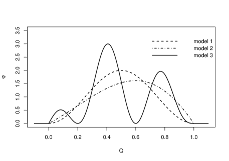
For each model $\mathcal{M}_{i}$, $1\leq i\leq 3$, we have computed the estimator and its corrected version presented in section 5.1 from independent design (data with uniform distribution on $Q$ denoted by $\mathcal{U}_{Q}$) and from Markov design. In the Markov case, the dataset is generated according to the Metropolis-Hastings algorithm with proposition kernel

$$P_{r}(x,dy)=\mathcal{U}_{[x-\varepsilon,x+\varepsilon]^{d}}(dy),$$

with $\varepsilon=0.2$ and target measure $\mathcal{U}_{Q}$. The Markov chain that results from this Metropolis-Hastings algorithm satisfies (A4). Indeed first note that, the kernel $P^{6}(x,dy)$ has a density which is lower bounded on $[0,1]^{2d}$ by a positive number (because $6\varepsilon>1$ and $\varphi(x)/\varphi(y)$ is lower bounded on $[0,1]^{2d}$), i.e., starting from any $x$ and waiting enough time will guarantee that any region is attained by the chain with positive probability. In other words, the uniform Doeblin condition holds for the chains $(X_{mk+1})_{k\geqslant 1}$ with the Lebesgue measure. Applying Theorem 16.0.2, page 394, in Meyn and Tweedie (2009), we obtain that the return time to $A$ of this chain, which is larger than the return time of the initial chain, has an exponential moment.

Independent and Markov designs have thus not been generated according to the same simulation model but share the same distribution, which makes them comparable. This will allow us to evaluate how the Markovian dependency impacts the performance of the methods. For the sake of reference, we have also computed the Monte Carlo estimator

$$\widehat{I}_{\text{mc}}=n^{-1}\sum_{i=1}^{n}\frac{\varphi(X_{i})}{\pi(X_{i})},$$

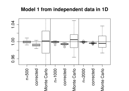
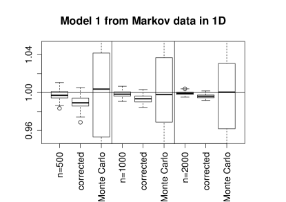
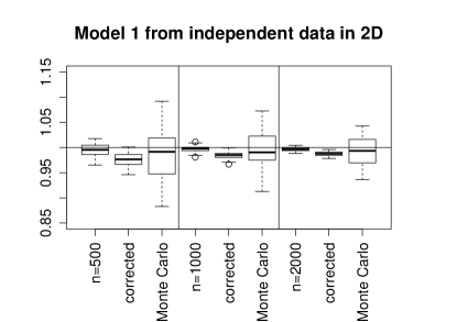
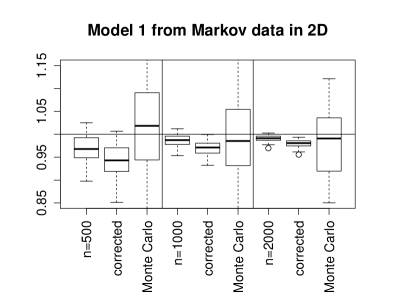
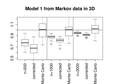
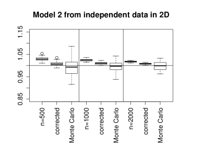
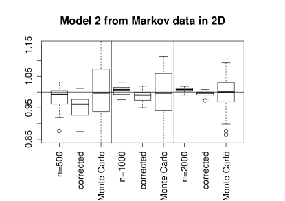
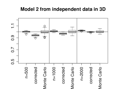
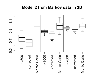
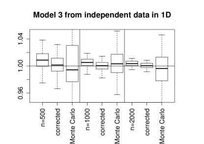
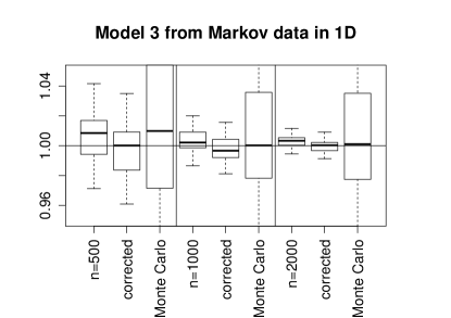
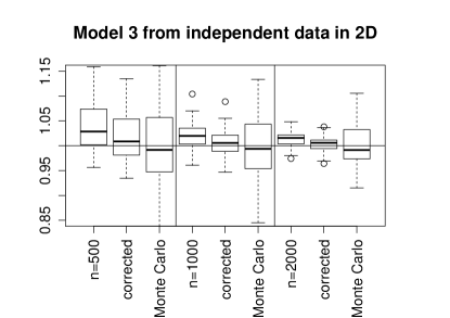
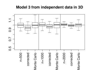
which can only be done in a simulation study where the distribution $\pi$ is known, and not from real data. Furthermore, we have investigated various sample sizes ($n=500$, $n=1\,000$ and $n=2\,000$) and different dimensions ($d=1$, $d=2$ and $d=3$). All the numerical results over $50$ independent replicates are provided in Figures 2 (model $\mathcal{M}_{1}$), 3 (model $\mathcal{M}_{2}$) and 4 (model $\mathcal{M}_{3}$). In order to make this numerical study reproducible, the R scripts implemented to generate datasets and estimate the integrals of interest are available at the webpage http://iecl.univ-lorraine.fr/~Romain.Azais/.

Figure 2: Boxplots of $\widehat{I}_{\text{ks}}$, $\widehat{I}_{\text{ks}}^{c}$ and $\widehat{I}_{\text{mc}}$ computed from $50$ replicates for model $\mathcal{M}_{1}$ in dimension $d=1$ (top), $d=2$ (middle) and $d=3$ (bottom) from independent data (left) and Markov data (right).

Figure 3: Boxplots of $\widehat{I}_{\text{ks}}$, $\widehat{I}_{\text{ks}}^{c}$ and $\widehat{I}_{\text{mc}}$ computed from $50$ replicates for model $\mathcal{M}_{2}$ in dimension $d=1$ (top), $d=2$ (middle) and $d=3$ (bottom) from independent data (left) and Markov data (right).

Figure 4: Boxplots of $\widehat{I}_{\text{ks}}$, $\widehat{I}_{\text{ks}}^{c}$ and $\widehat{I}_{\text{mc}}$ computed from $50$ replicates for model $\mathcal{M}_{3}$ in dimension $d=1$ (top), $d=2$ (middle) and $d=3$ (bottom) from independent data (left) and Markov data (right).

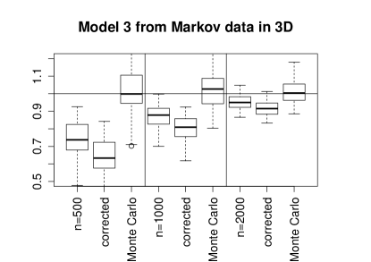First, estimators $\widehat{I}_{\text{ks}}$ and $\widehat{I}_{\text{ks}}^{c}$ have similar dispersions, but the corrected version is more accurate in most cases and should be promoted. Unsurprisingly, the results are better in terms of bias and variance when estimation of the design distribution is computed from independent data rather from Markov data. In addition, the accuracy deteriorates when the dimension increases. For too small samples, the integral is underestimated (see for example models $\mathcal{M}_{1}$ and $\mathcal{M}_{2}$ in dimensions $2$ and $3$), in particular in the Markov framework (see model $\mathcal{M}_{3}$ in dimension $3$). Numerical results are quite similar for models $\mathcal{M}_{1}$ and $\mathcal{M}_{2}$, which states that the method is not sensitive to skewness. As expected, quality is a little lower for $\mathcal{M}_{3}$. In the $3$ considered models, the Monte Carlo estimator $\widehat{I}_{\text{mc}}$ presents no bias but a large dispersion in comparison with $\widehat{I}_{\text{ks}}$ and $\widehat{I}_{\text{ks}}^{c}$, especially in the Markov framework where the dataset does not exactly follow the distribution $\pi$. The numerical study shows that the methodology is very efficient and applicable in various contexts, in particular compared to Monte Carlo methods that achieve worse results in terms of variance and can not be applied in a statistical framework. Nevertheless, additional numerical experiments point out that both estimators present some bias when function $\varphi$ is not continuous.

As stated in Theorem 8, the shape of the function $\pi$ (and secondarily $\varphi$) plays an important role in the convergence rate of $\widehat{I}_{\text{ks}}$: the smoother the better. Hence, the situation when $\pi$ is the uniform density on $Q$ is far from being easy (as the function is not even continuous). Continuity of $\pi$ is no remedy as it implies the cancellation of $\pi$ at the border and therefore provides too few points near the border. One solution is to consider points that lie slightly outside $Q$, say in $\tilde{Q}\supset Q$, in order to stabilize the estimation of $\pi$ at the border of $Q$. Then compute the kernel estimator $\tilde{\pi}$ using all these points, and finally calculate

$$\tilde{I}_{\text{ks}}=n^{-1}\sum_{i=1}^{n}\frac{\varphi(X_{i})\mathbb{1}_{\{X_{i}\in Q\}}}{\tilde{\pi}(X_{i})}.$$

In the applications where only points in $Q$ are given, one might prefer to consider a different set $Q$, slightly smaller than the original, in order to implement the previous method. If collecting the points has not been done, it might be appropriate to allow the sensor capturing data to get out of $Q$.

5.3 Real data analysis

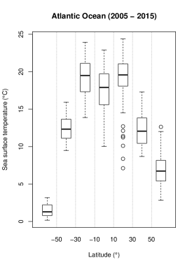
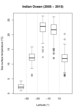
The U.S. National Centers for Environmental Information (NCEI) are parts of National Oceanic and Atmospheric Administration (NOAA). NCEI form the world’s largest provider of weather and climate data. The real data analysis presented in the present paper is based on sea surface temperatures obtained all around the world between 2005 and 2015 from profiling floats (PFL dataset) and available on NCEI’s website. Sea surface temperatures have a large influence on climate and weather and are therefore used in analyses of climate change. The dataset investigated in this article contains about $1.3$M data and is fully described in Table 1 and Figure 5. Data preprocessing has been implemented in Python, while estimation and data analysis have been made with R.

Total
1 343 094
Ocean
Pacific		Atlantic		Indian
727 135		336 180		279 779
Year		Year		Year
2005 (min)	2015 (max)	2005 (min)	2015 (max)	2005 (min)	2015 (max)
35 773	86 961	16 242	45 488	14 134	33 049

Table 1: Size of the sub-datasets extracted from PFL dataset between 2005 and 2015.

Figure 5: Visualization of the 1 343 094 points of PFL dataset between 2005 and 2015. Oceans are distinguished using gray shades (darker to lighter: Pacific, Atlantic, Indian).

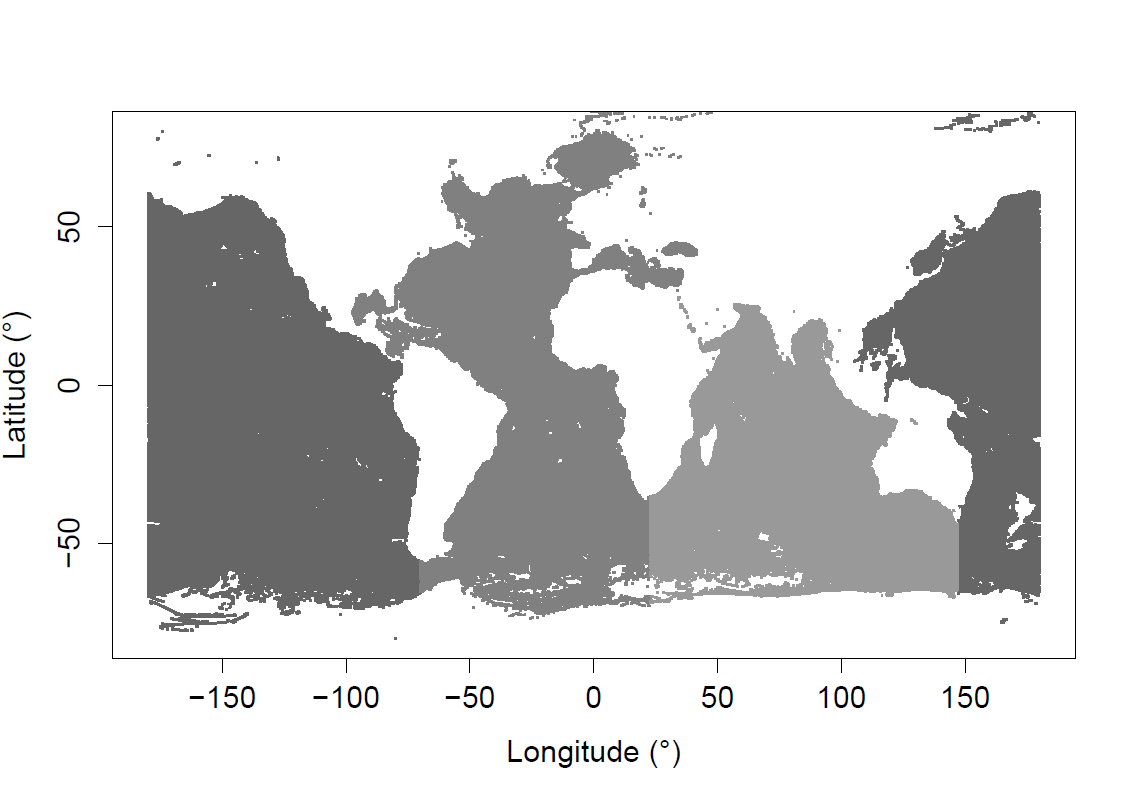
The database of interest consists of spatiotemporal data obtained from measure instruments with unpredictable trajectories, which makes them hardly tractable. We focus here on the estimation of the average sea surface temperature for a given period of time, between 2005 and 2015, and for some given areas in the 3 major oceans. Areas considered in this paper are delimited by the latitude: more than $50^{\circ}$ (North region), $[30^{\circ},50^{\circ}]$, $[10^{\circ},30^{\circ}]$ (North Tropical region), $[-10^{\circ},10^{\circ}]$ (Equatorial region), $[-30^{\circ},-10^{\circ}]$ (South Tropical region), $[-30^{\circ},-50^{\circ}]$ and less than $-50^{\circ}$ (South region). For each mentioned spatial region, we have estimated the average sea surface temperature over each month by the corrected algorithm presented in section 5.1. This technique is fully adapted to the problem at hand because measurement locations follow erratic trajectories with unknown distribution.

Local average sea surface temperatures for the 3 oceans are presented in Figure 6. One obtains temperature patterns according to the location on the North-South axis. One may observe that the variability of sea surface temperatures in a given region over $11$ years is weak compared to the variations in latitude, especially for the Pacific Ocean. In other words, the temperature mainly depends on the latitude, rather on the period of the year. Unsurprinsingly, sea surface temperatures are the highest under the Equator and near the Tropics, where Earth receives the most direct sunlight.

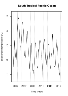
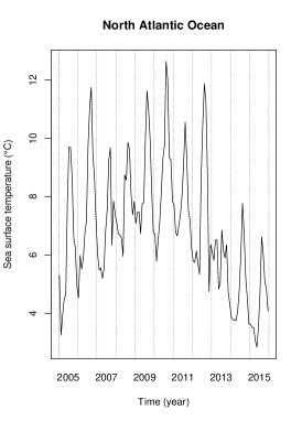
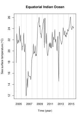
In Figure 7, we present time series over $11$ years of average sea surface temperatures in $3$ regions: South Tropical Pacific Ocean (latitude between $-30^{\circ}$ and $-10^{\circ}$), North Atlantic Ocean (latitude between $50^{\circ}$ and $60^{\circ}$) and Equatorial Indian Ocean (latitude between $-10^{\circ}$ and $10^{\circ}$). First, it should be noted that we observe an expected seasonal effect on sea surface temperatures of South Pacific and North Atlantic Oceans: the highest temperatures occur in January and February in the Southern Hemisphere, while they occur in August and September in North Atlantic Ocean. In addition, we note a general decrease in sea surface temperature in Southern Pacific between 2006 and 2009 followed by a stable period. This phenomenon has been taken into account in simulations proposed in Kosaka and Xie (2013). In particular, they show that recent cooling in Pacific Ocean is tied to recent global-warming hiatus. One may also remark that temperature in North Atlantic Ocean has decreased recently. Indeed, there is a region of cooling in the Northern Atlantic. Rahmstorf et al. (2015) suggest that this cooling may be due to changes in the Atlantic meridional overturning circulation in the late twentieth century. Finally we point out that Equatorial Indian Ocean has tended to warm for at least $10$ years. According to Roxy et al. (2014), this warming begun more than a century ago and is linked to the El Niño – Southern Oscillation periodical phenomenon.

Figure 6: Average sea surface temperatures according to the latitude of the considered area for the 3 major oceans. Each boxplot has been computed from $11\times 12=132$ estimates of the average temperature for each month of each year between 2005 and 2015.

Figure 7: Times series of sea surface temperature in some specific areas of the 3 major oceans between 2005 and 2015. Latitude between $-30^{\circ}$ and $-10^{\circ}$ for South Tropical Pacific Ocean (top), $50^{\circ}$ and $60^{\circ}$ for North Atlantic Ocean (middle), and $-10^{\circ}$ and $10^{\circ}$ for Equatorial Indian Ocean (bottom).

Appendix A Regeneration-based bounds for expectations

We employed the Nummelin splitting technique in order to exploit the independence between the blocks $B_{k}$, $k\in\mathbb{N}^{*}$, as described in section 2 of the associated paper. We have however taken care of giving conditions on the moments $\tau_{A}$ of the original chain $(X_{i})_{i\in\mathbb{N}}$ rather than on the moments $\theta_{a}$ of the split chain $(Z_{i})_{i\in\mathbb{N}}$.

Define, for any $p>0$,

$$\xi(p)=\sup_{x\in A}\mathbb{E}_{x}[\tau_{A}^{p}].$$

We start with a lemma relating moments of $\theta_{a}$ to moments of $\tau_{A}$.

Lemma 9.

Let $(X_{i})_{i\in\mathbb{N}}$ be a Markov chain satisfying (5). Then, for any $x_{0}\in\mathcal{E}$, $p\geqslant 1$,

$$\mathbb{E}_{x_{0}}[\theta_{a}^{p}]^{1/p}\leqslant\frac{1}{e^{\lambda_{0}/{p}}-1}\xi(p)^{1/p}+\mathbb{E}_{x_{0}}[\tau_{A}^{p}]^{1/p}$$ (25)

$$\mathbb{E}_{a}[\theta_{a}^{p}]^{1/p}\leqslant\lambda_{0}^{-1}\frac{e^{\lambda_{0}/{p}}}{e^{\lambda_{0}/{p}}-1}\xi(p)^{1/p}.$$ (26)

Proof.

We start by showing (25). Suppose that $\mathbb{E}_{x_{0}}[\tau_{A}^{p}]<+\infty$ and $\sup_{x\in A}\mathbb{E}_{x}[\tau_{A}^{p}]<+\infty$, if not, the stated inequality is obviously satisfied. By the Minkowski inequality, we have

$$\mathbb{E}_{x_{0}}[\theta_{a}^{p}]^{1/p} \leqslant\mathbb{E}_{x_{0}}[(\theta_{a}-\tau_{A})^{p}]^{1/p}+\mathbb{E}_{x_{0}}[\tau_{A}^{p}]^{1/p}$$

$$=\mathbb{E}_{x_{0}}[(\theta_{a}-\tau_{A})^{p}\mathbb{1}_{\{\theta_{a}>\tau_{A}\}}]^{1/p}+\mathbb{E}_{x_{0}}[\tau_{A}^{p}]^{1/p}.$$

Let $\mathscr{F}_{\tau_{A}}$ denote the $\sigma$-field of the past before $\tau_{A}$ and note that ${\{\theta_{a}>\tau_{A}\}}$ is $\mathscr{F}_{\tau_{A}}$-measurable. By the strong Markov property, it holds

$$\mathbb{E}_{x_{0}}[(\theta_{a}-\tau_{A})^{p}\mathbb{1}_{\{\theta_{a}>\tau_{A}\}}|\mathscr{F}_{\tau_{A}}]=\mathbb{E}_{x_{0}}[(\theta_{a}-\tau_{A})^{p}|\mathscr{F}_{\tau_{A}}]\mathbb{1}_{\{\theta_{a}>\tau_{A}\}}\leqslant\mathbb{1}_{\{\theta_{a}>\tau_{A}\}}\sup_{x\in A}\mathbb{E}_{x}[\theta_{a}^{p}].$$

Hence, setting $\gamma=\sup_{x\in A}\mathbb{E}_{x}[\theta_{a}^{p}]^{1/p}$, and because $\lambda_{0}=\mathbb{P}_{x_{0}}(\theta_{a}=\tau_{A})=\mathbb{P}_{x_{0}}(Y_{\tau_{A}}=1)$,

$$\mathbb{E}_{x_{0}}[\theta_{a}^{p}]^{1/p} \leqslant\gamma(1-\lambda_{0})^{1/p}+\mathbb{E}_{x_{0}}[\tau_{A}^{p}]^{1/p}.$$ (27)

In particular, it follows that

$$(1-(1-\lambda_{0})^{1/p})\gamma \leqslant\sup_{x\in A}\mathbb{E}_{x}[\tau_{A}^{p}]^{1/p}.$$

Thus, (27) becomes

$$\mathbb{E}_{x_{0}}[\theta_{a}^{p}]^{1/p} \leqslant(1-\lambda_{0})^{1/p}(1-(1-\lambda_{0})^{1/p})^{-1}\sup_{x\in A}\mathbb{E}_{x}[\tau_{A}^{p}]^{1/p}+\mathbb{E}_{x_{0}}[\tau_{A}^{p}]^{1/p},$$ (28)

and we obtain (25) by using $1-\lambda_{0}\leqslant e^{-\lambda_{0}}$. To get (26), note that for every $x_{0}\in A$,

$$\mathbb{E}_{x_{0}}[\theta_{a}^{p}\mathbb{1}_{\{Y_{0}=1\}}]=\lambda_{0}\mathbb{E}_{a}[\theta_{a}^{p}].$$

It follows that $\mathbb{E}_{a}[\theta_{a}^{p}]\leqslant\lambda_{0}^{-1}\mathbb{E}_{x_{0}}[\theta_{a}^{p}]$ and we get the result from (25), taking the supremum over $A$. ∎

We shall need also the following extension of (10).

Lemma 10.

Let $(X_{i})_{i\in\mathbb{N}}$ be a Markov chain satisfying (2), (3) and (5). For any measurable function $h:\cup_{n\geqslant 1}\mathbb{R}^{n}\rightarrow\mathbb{R}$ such that $\mathbb{E}_{\pi}[h(X_{1},...X_{\theta_{a}})]<+\infty$, (for any $n$ the restriction of $h$ to $\mathbb{R}^{n}$ is measurable), we have

$$\alpha_{0}\mathbb{E}_{\pi}[h(X_{1},...X_{\theta_{a}})] =\mathbb{E}_{a}\Big{[}\sum_{i=1}^{\theta_{a}}h(X_{i},...X_{\theta_{a}})\Big{]}.$$ (29)

In particular, for any $p>0$,

$$\alpha_{0}\mathbb{E}_{\pi}[\theta_{a}^{p}] \leqslant\mathbb{E}_{a}[\theta_{a}^{p+1}]\leqslant(p+1)\alpha_{0}\mathbb{E}_{\pi}[\theta_{a}^{p}].$$ (30)

Proof.

Having (2), (3) and (5) we can use the formula (10). Define $g(x)=\mathbb{E}_{x}[h(X_{1},...X_{\theta_{a}})]$ and remark that, by the Markov property and the fact that $\{i<\theta_{a}\}$ is $\mathscr{F}_{i}$-measurable,

$$\mathbb{E}_{a}(g(X_{i})\mathbb{1}_{\{i<\theta_{a}\}})=\mathbb{E}_{a}(h(X_{i+1},...X_{\theta_{a}})\mathbb{1}_{\{i<\theta_{a}\}}),$$

$$g(X_{\theta_{a}})=\mathbb{E}_{a}(h(X_{1},...X_{\theta_{a}})).$$

Then using (10) with $g$, we get

$$\alpha_{0}\mathbb{E}_{\pi}[h(X_{1},...X_{\theta_{a}})] =\alpha_{0}\pi(g)$$

$$=\mathbb{E}_{a}\Big{[}\sum_{i=1}^{\theta_{a}}g(X_{i})\Big{]}$$

$$=\mathbb{E}_{a}\Big{[}\sum_{i=1}^{{\theta_{a}}-1}h(X_{i+1},...X_{\theta_{a}})\Big{]}+\mathbb{E}_{a}\Big{[}h(X_{1},...X_{{\theta_{a}}})\Big{]}$$

$$=\mathbb{E}_{a}\Big{[}\sum_{i=1}^{{\theta_{a}}}h(X_{i},...X_{\theta_{a}})\Big{]}.$$

Concerning the second statement, we use the fact that $1+2^{p}+\dots\theta_{a}^{p}\geqslant\int_{0}^{\theta_{a}}x^{p}dx=\frac{\theta_{a}^{p+1}}{p+1}$ to write

$$\tfrac{1}{p+1}\mathbb{E}_{a}[\theta_{a}^{p+1}]\leqslant\mathbb{E}_{a}\big{[}\sum_{i=1}^{\theta_{a}}i^{p}\big{]}\leqslant\mathbb{E}_{a}[\theta_{a}^{p+1}].$$

We conclude by using (29) with $h(x_{1},\dots x_{k})=k^{p}$, to show that the middle term is $\alpha_{0}\mathbb{E}_{\pi}[\theta_{a}^{p}]$. ∎

Lemma 11.

Let $(X_{i})_{i\in\mathbb{N}}$ be a Markov chain satisfying (2), (3) and (5). For any $p>2$, there exists $C>0$ (depending on $p$, $\lambda_{0}$, $\alpha_{0}$) such that for any measurable function $f$,

$$\mathbb{E}_{a}\Big{[}\Big{(}\sum_{i=1}^{\theta_{a}}f(X_{i})\Big{)}^{2}\Big{]} \leqslant C\left(\xi(p)^{2}\pi(f^{2})+\xi(p)\mathbb{E}_{\pi}[f(X_{0})^{2}\tau_{A}^{p}]\right).$$

Proof.

Suppose that $f\geqslant 0$. If not, take $|f|$ instead of $f$. In what follows, we use the convention that empty sums equal $0$. Applying Lemma 10 with

$$h(x_{i},\ldots x_{k})=\Big{(}\sum_{j=1}^{k}f(x_{j})\Big{)}^{2}-\Big{(}\sum_{j=2}^{k}f(x_{j})\Big{)}^{2}=f(x_{i})^{2}+2f(x_{i})\sum_{j=2}^{k}f(x_{j}),$$

we get that

$$\mathbb{E}_{a}\Big{[}\Big{(}\sum_{i=1}^{\theta_{a}}f(X_{i})\Big{)}^{2}\Big{]} =\mathbb{E}_{a}\Big{[}\sum_{i=1}^{\theta_{a}}h(X_{i},\ldots X_{\theta_{a}})\Big{]}$$

$$=\alpha_{0}\mathbb{E}_{\pi}\Big{[}f(X_{1})\Big{(}f(X_{1})+2\sum_{i=2}^{\theta_{a}}f(X_{i})\Big{)}\Big{]}$$

$$=\alpha_{0}\left(\pi(f^{2})+2\mathbb{E}_{\pi}\Big{[}f(X_{1})\sum_{i=2}^{\theta_{a}}f(X_{i})\Big{]}\right).$$

For any $p>2$, the second term is bounded as follows

$$\mathbb{E}_{\pi}\Big{[}f(X_{1})\sum_{i=2}^{{\theta_{a}}}f(X_{i})\Big{]} =\sum_{i\geqslant 2}\mathbb{E}_{\pi}\Big{[}\mathbb{1}_{i\leqslant{\theta_{a}}}f(X_{1})f(X_{i})\Big{]}$$

$$\leqslant\sum_{i\geqslant 2}\mathbb{E}_{\pi}\Big{[}i^{-p/2}\theta_{a}^{p/2}\,f(X_{1})f(X_{i})\Big{]}$$

$$\leqslant\sum_{i\geqslant 2}i^{-p/2}\mathbb{E}_{\pi}\Big{[}f(X_{1})^{2}\theta_{a}^{p}\Big{]}^{1/2}\mathbb{E}_{\pi}\Big{[}f(X_{i})^{2}\Big{]}^{1/2}$$

$$=\left(\sum_{i\geqslant 2}i^{-p/2}\right)\mathbb{E}_{\pi}\Big{[}f(X_{1})^{2}\theta_{a}^{p}\Big{]}^{1/2}\mathbb{E}_{\pi}\Big{[}f(X_{1})^{2}\Big{]}^{1/2}$$

$$\leqslant\left(\frac{2}{p-2}\right)\mathbb{E}_{\pi}\Big{[}f(X_{1})^{2}\theta_{a}^{p}\Big{]},$$

where we have used $\sum_{i\geqslant 2}i^{-p/2}\leqslant\int_{1}^{+\infty}x^{-p/2}dx$. If $\widetilde{\theta}_{a}$ is the first time $k\geqslant 2$ such $Z_{k}\in a$, it holds

$$\mathbb{E}_{\pi}\Big{[}f(X_{1})^{2}\theta_{a}^{p}\Big{]}\leqslant\mathbb{E}_{\pi}\Big{[}f(X_{1})^{2}\widetilde{\theta}_{a}^{p}\Big{]}=\mathbb{E}_{\pi}\Big{[}f(X_{0})^{2}(\theta_{a}^{p}+1)\Big{]}\leqslant 2\mathbb{E}_{\pi}\Big{[}f(X_{0})^{2}\theta_{a}^{p}\Big{]}.$$

Applying Lemma 9, equation (25), and using that for every $a,b\geqslant 0$, and $p>1$, $(a+b)^{p}\leqslant 2^{p-1}(a^{p}+b^{p})$, we get

$$\mathbb{E}_{\pi}\Big{[}f(X_{0})^{2}\theta_{a}^{p}\Big{]}\leqslant 2^{p-1}\left(\frac{1}{(e^{\lambda_{0}/{p}}-1)^{p}}\xi(p)\pi(f^{2})+\mathbb{E}_{\pi}\left[f(X_{0})^{2}\tau_{A}^{p}\right]\right).$$

Bringing everything together, we get

$$\mathbb{E}_{a}\Big{[}\Big{(}\sum_{i=1}^{\theta_{a}}f(X_{i})\Big{)}^{2}\Big{]}\leqslant\alpha_{0}\left(\pi(f^{2})+\frac{2^{p+2}}{p-2}\left(\frac{1}{(e^{\lambda_{0}/{p}}-1)^{p}}\xi(p)\pi(f^{2})+\mathbb{E}_{\pi}\left[f(X_{0})^{2}\tau_{A}^{p}\right]\right)\right).$$

This leads to the stated result. ∎

Theorem 12.

Let $(X_{i})_{i\in\mathbb{N}}$ be a Markov chain satisfying (2), (3) and (5). There exists $C>0$ (depending on $p$, $\lambda_{0}$, $\alpha_{0}$) such that, for any measurable function $g$ with $\pi(g)=0$, any $n\geqslant 1$ and $p>2$,

$$\mathbb{E}_{\pi}\Big{[}\Big{(}\sum_{i=1}^{n}g(X_{i})\Big{)}^{2}\Big{]}\leqslant nC\left(\xi(p)^{2}\pi(g^{2})+\xi(p)\mathbb{E}_{\pi}[g(X_{0})^{2}\tau_{A}^{p}]\right).$$

Proof.

Defining the blocks sums as (see equation (9))

$$G_{k} =\sum_{i={\theta_{a}}(k)+1}^{{\theta_{a}}(k+1)}g(X_{i}),$$

(in this whole section we set $\sum\nolimits_{a}^{b}=0$ if $b<a$) $G_{k}$ is an i.i.d. sequence and one has

$$\sum_{i=1}^{n}g(X_{i}) =\sum_{i=1}^{{\theta_{a}}\wedge n}g(X_{i})+\sum_{k=1}^{l_{n}-1}G_{k}+\mathbb{1}_{{\theta_{a}}\leqslant n}\sum_{i={\theta_{a}}(l_{n})+1}^{n}g(X_{i})$$

where $l_{n}$ is the number of times $Z_{i}$ visits $a$ before $n$, i.e.,

$$l_{n}=\sum_{i=1}^{n}\mathbb{1}_{\{Z_{i}\in a\}}.$$ (31)

As the chain has been split into independent blocks, the process $L\mapsto\sum_{k=1}^{L}G_{k}$ is a martingale. The sequence $(l_{n})$ is random and is expected to be of order $n$. Since $l_{n}\leqslant n$, following Bertail and Clémençon (2011), page 21, we have

$$\Big{|}\sum_{i=1}^{n}g(X_{i})\Big{|}\leqslant\sum_{i=1}^{{\theta_{a}}\wedge n}f(X_{i})+\max_{1\leqslant L\leqslant n}\Big{|}\sum_{k=1}^{L}G_{k}\Big{|}+\mathbb{1}_{{\theta_{a}}\leqslant n}\sum_{i={\theta_{a}}(l_{n})+1}^{n}f(X_{i}),$$

where $f=|g|$ (considering $f$ instead of $g$ will help later for the treatment of the concerned terms). By the Minkowski inequality, denoting by $\|\cdot\|_{2}$ the $L_{2}(\mathbb{P}_{\pi})$ norm, we have

$$\Big{\|}\sum_{i=1}^{n}g(X_{i})\Big{\|}_{2} \leqslant\Big{\|}\sum_{i=1}^{{\theta_{a}}\wedge n}f(X_{i})\Big{\|}_{2}+\Big{\|}\max_{1\leqslant L\leqslant n}\Big{|}\sum_{k=1}^{L}G_{k}\Big{|}\Big{\|}_{2}+\Big{\|}\sum_{i={\theta_{a}}(l_{n})+1}^{n}f(X_{i})\Big{\|}_{2}.$$ (32)

Using Doob’s inequality, we have

$$\mathbb{E}_{\pi}\max_{1\leqslant L\leqslant n}\Big{|}\sum_{k=1}^{L}G_{k}\Big{|}^{2}\leqslant 4n\mathbb{E}_{\pi}[|G_{1}|^{2}]=4n\mathbb{E}_{a}\Big{[}\Big{(}\sum_{i=1}^{\theta_{a}}g(X_{i})\Big{)}^{2}\Big{]},$$

then, from Lemma 11, we get for every $p>2$ that there exist $\widetilde{C}$ such that

$$\mathbb{E}_{\pi}\max_{1\leqslant L\leqslant n}\Big{|}\sum_{k=1}^{L}G_{k}\Big{|}^{2}\leqslant 4n\widetilde{C}\left(\xi(p)^{2}\pi(g^{2})+\xi(p)\mathbb{E}_{\pi}[g(X_{0})^{2}\tau_{A}^{p}]\right)$$

This is also a crude bound for the third term in (32) since

$$\mathbb{E}_{\pi}\Big{[}\Big{(}\sum_{i={\theta_{a}}(l_{n})+1}^{n}f(X_{i})\Big{)}^{2}\Big{]} \leqslant\mathbb{E}_{\pi}\Big{[}\Big{(}\sum_{i={\theta_{a}}(l_{n})+1}^{{\theta_{a}}(l_{n}+1)}f(X_{i})\Big{)}^{2}\Big{]}=\mathbb{E}_{a}\Big{[}\Big{(}\sum_{i=1}^{\theta_{a}}f(X_{i})\Big{)}^{2}\Big{]}.$$

Now we consider the first term in (32). Using Lemma 10 with

$$h(x_{1},\ldots x_{k})=\Big{(}\sum_{j=1}^{k\wedge n}f(x_{j})\Big{)}^{2},$$

we get

$$\mathbb{E}_{\pi}\Big{[}\Big{(}\sum_{j=1}^{\theta_{a}\wedge n}f(X_{j})\Big{)}^{2}\Big{]} =\alpha_{0}^{-1}\mathbb{E}_{a}\Big{[}\sum_{i=1}^{\theta_{a}}\Big{(}\sum_{j=i}^{\theta_{a}\wedge n}f(X_{j})\Big{)}^{2}\Big{]}$$

$$=\alpha_{0}^{-1}\mathbb{E}_{a}\Big{[}\sum_{i=1}^{\theta_{a}\wedge n}\Big{(}\sum_{j=i}^{\theta_{a}\wedge n}f(X_{j})\Big{)}^{2}\Big{]}$$

$$\leqslant n\alpha_{0}^{-1}\mathbb{E}_{a}\Big{[}\Big{(}\sum_{j=1}^{\theta_{a}}f(X_{j})\Big{)}^{2}\Big{]}$$

$$\leqslant n\mathbb{E}_{a}\Big{[}\Big{(}\sum_{j=1}^{\theta_{a}}f(X_{j})\Big{)}^{2}\Big{]}.$$

We conclude again with Lemma 11. ∎

Appendix B Proofs of section 3

B.1 Proof of Lemma 1

We start by proving (12). Define $k=\lfloor s\rfloor$. From the Taylor formula with integral remainder applied to $g(t)=\psi(x-tu)$, we get

$$\psi(x-hu)-\psi(x) =\sum_{j=1}^{k-1}\frac{h^{j}}{j!}g^{(j)}(0)+\int_{0}^{h}g^{(k)}(t)\frac{(h-t)^{k-1}}{(k-1)!}dt$$

$$=\sum_{j=1}^{k}\frac{h^{j}}{j!}g^{(j)}(0)+\int_{0}^{h}(g^{(k)}(t)-g^{(k)}(0))\frac{(h-t)^{k-1}}{(k-1)!}dt.$$

The first term is a polynomial in $u$ which vanishes after integration with respect to $K$ as by assumption, $K$ is orthogonal to the first non-constant polynomial of degree $j\leq\lfloor s\rfloor$. Using the chain rule to compute $g^{(k)}$ and using basic inequalities with some combinatorics, we obtain that there exists a constant $C$ (depending only on $k$ and $d$) such that for every $t\in\mathbb{R}$,

$$|g^{(k)}(t)-g^{(k)}(0)|\leqslant C|u|_{1}^{k}\sum_{l\in\mathcal{P}_{k}}|\psi^{(l)}(x-tu)-\psi^{(l)}(x)|,$$

where $\mathcal{P}_{k}=\{(l_{1},\ldots l_{d})\in\mathbb{N}^{d}\,:\,\sum_{i=1}^{d}l_{i}=k\}$. It follows that

$$\Big{|}\int_{0}^{h}(g^{(k)}(t)-g^{(k)}(0))\frac{(h-t)^{k-1}}{(k-1)!}dt\Big{|} \leqslant\frac{h^{k-1}C}{(k-1)!}\sum_{l\in\mathcal{P}_{k}}\int_{0}^{h}|\psi^{(l)}(x-tu)-\psi^{(l)}(x)|\,|u|_{1}^{k}dt.$$

Hence

$$\Big{|}\int\left(\psi(x-hu)-\psi(x)\right)K(u)du\Big{|}\leqslant\frac{h^{k-1}C}{(k-1)!}\sum_{l\in\mathcal{P}_{k}}\int_{0}^{h}\int|\psi^{(l)}(x-tu)-\psi^{(l)}(x)|\,|u|_{1}^{k}\,|K(u)|\,du\,dt$$

and by the generalized Minkowski inequality (Folland, 1999, page 194),

$$\big{\|}\psi-\psi_{h}\big{\|}_{L_{q}(\pi)} \leqslant\frac{h^{k-1}C}{(k-1)!}\sum_{l\in\mathcal{P}_{k}}\int\int\left(\int|\psi^{(l)}(x-tu)-\psi^{(l)}(x)|^{q}|u|_{1}^{qk}|K(u)|^{q}\mathbb{1}_{0\leqslant t\leqslant h}\pi(x)dx\right)^{1/q}\!\!\!\!du\,dt$$

$$\leqslant\frac{h^{k-1}C}{(k-1)!}M_{1}\pi_{\infty}^{1/q}\sum_{l\in\mathcal{P}_{k}}\int\left(|tu|_{1}^{q(s-k)}|u|_{1}^{qk}|K(u)|^{q}\right)^{1/q}\mathbb{1}_{0\leqslant t\leqslant h}du\,dt$$

$$=\frac{h^{s}C}{(k-1)!(s-k+1)}M_{1}\pi_{\infty}^{1/q}\,\#\{\mathcal{P}_{k}\}\int|u|_{1}^{s}|K(u)|du.$$

This implies (12).

To show (13), it suffices to provide an upper-bound proportional to $h^{s}$ and another one proportional to $h^{r}$. Because $|\pi(\psi-\psi_{h})|\leqslant\pi(|\psi-\psi_{h}|)$, applying (12) with $q=1$, we obtain the upper-bound $C_{1}M_{1}\pi_{\infty}h^{s}$. By Fubini’s theorem and using the symmetry about $0$ of $K$, it holds

$$\int\pi(x)\psi_{h}(x)dx=\int\psi(x)\pi_{h}(x)dx.$$ (33)

Hence, introducing the probability density $\widetilde{\psi}(y)=\left(\int|\psi(x)|dx\right)^{-1}|\psi(y)|$, $y\in\mathbb{R}^{d}$, we find

$$\left|\int\pi(x)(\psi(x)-\psi_{h}(x))dx\right| =\left|\int\psi(x)(\pi(x)-\pi_{h}(x))dx\right|$$

$$\leqslant\left(\int|\psi(x)|dx\right)\int\widetilde{\psi}(x)\left|\pi(x)-\pi_{h}(x)\right|dx$$

$$=\left(\int|\psi(x)|dx\right)\left\|\pi-\pi_{h}\right\|_{L_{1}(\widetilde{\psi})}.$$

Applying (12) with $\widetilde{\psi}$ and $\pi$ in place of $\pi$ and $\psi$ respectively, we get the bound $\widetilde{C}_{1}M_{2}\psi_{\infty}h^{r}$, for some $\widetilde{C}_{1}>0$ depending on $K$ and $r$. Equation (13) is then deduced from these two bounds.

B.2 Proof of Proposition 3

For any $f$ and $\widetilde{f}$ in $\mathcal{F}_{1}\times\ldots\times\mathcal{F}_{d}$, we have

$$|\Psi(f)-\Psi(\widetilde{f}))| \leqslant\sum_{j=1}^{d}C_{j}(F)|f_{j}-\widetilde{f}_{j}|.$$ (34)

Let us first prove that $G$ is an envelope for $\mathcal{G}$. Applying (34) with $f_{0}$ in place of $\widetilde{f}$, we get that $2\sum_{j=1}^{d}C_{j}(F)F_{j}$ is an envelope for the class $\mathcal{G}-\Psi(f_{0})$. As a result $G$ is an envelope for the class $\mathcal{G}$. The envelope property is proved.

Let $Q$ be such that $Q(G^{2})<+\infty$. Define the following probability measures on $\mathcal{X}$,

$$dQ_{j}=q_{j}^{-2}C_{j}(F)^{2}\,dQ,\qquad\text{with }q_{j}^{2}=\int C_{j}(F)^{2}\,dQ.$$

Note that $q_{j}<+\infty$ is implied by $Q(G^{2})<+\infty$. Let $\mathcal{C}_{j}$ denote a set of functions forming an $\epsilon\|F_{j}\|_{L_{2}(Q_{j})}$-covering of the metric space $(\mathcal{F}_{j},L_{2}(Q_{j}))$. For $f=(f_{1},\ldots f_{d})\in\mathcal{F}_{1}\times\ldots\times\mathcal{F}_{d}$, there exists $\widetilde{f}=(\widetilde{f}_{1},\ldots\widetilde{f}_{d})\in\mathcal{C}_{1}\times\ldots\times\mathcal{C}_{d}$ such that, using (34) and the Minkowski inequality,

$$\|\Psi(f)-\Psi(\widetilde{f})\|_{L_{2}(Q)} \leqslant\sum_{j=1}^{d}\|(f_{j}-\widetilde{f}_{j}){C_{j}}(F)\|_{L_{2}(Q)}$$

$$\leqslant\sum_{j=1}^{d}q_{j}\|f_{j}-\widetilde{f}_{j}\|_{L_{2}(Q_{j})}$$

$$\leqslant\epsilon\sum_{j=1}^{d}q_{j}\|F_{j}\|_{L_{2}(Q_{j})}.$$

The number of possible $d$-uplets $(\widetilde{f}_{1},\ldots\widetilde{f}_{d})$ is at most $\prod_{j=1}^{d}\#\{\mathcal{C}_{j}\}$, thus

$$\mathcal{N}\Big{(}\mathcal{G},\,L_{2}(Q),\epsilon\sum_{j=1}^{d}q_{j}\|F_{j}\|_{L_{2}(Q_{j})}\Big{)}\leqslant\prod_{j=1}^{d}\mathcal{N}\left(\mathcal{F}_{j},\,L_{2}(Q_{j}),\,\epsilon\|F_{j}\|_{L_{2}(Q_{j})}\right).$$

We have

$$\int G(x)^{2}dQ \geqslant\int|\Psi(f_{0})|^{2}dQ+4\sum_{j=1}^{d}\int F_{j}^{2}{C_{j}}(F)^{2}\,dQ$$

$$\geqslant\sum_{j=1}^{d}\int F_{j}^{2}{C_{j}}(F)^{2}\,dQ$$

$$=\sum_{j=1}^{d}q_{j}^{2}\|F_{j}\|_{L_{2}(Q_{j})}^{2}.$$

Combining this with the Schwartz inequality gives

$$\sum_{j=1}^{d}q_{j}\|F_{j}\|_{L_{2}(Q_{j})} \leqslant d^{1/2}\left(\sum_{j=1}^{d}q_{j}^{2}\|F_{j}\|_{L_{2}(Q_{j})}^{2}\right)^{1/2}\leqslant d^{1/2}\|G\|_{L_{2}(Q)}.$$

Hence

$$\mathcal{N}\left(\mathcal{G},\,L_{2}(Q),\epsilon d^{1/2}\|G\|_{L_{2}(Q)}\right)\leqslant\prod_{j=1}^{d}\mathcal{N}\left(\mathcal{F}_{j},\,L_{2}(Q_{j}),\,\epsilon\|F_{j}\|_{L_{2}(Q_{j})}\right).$$

The VC class assumption on $\mathcal{F}_{j}$, with characteristics $(A_{j},v_{j})$, implies that the right hand side is smaller than $\varepsilon^{-(v_{1}+\dots+v_{d})}A_{1}^{v_{1}}\dots A_{d}^{v_{d}}$. This concludes the proof.

B.3 Proof of Proposition 4

The first statement is proved in van der Vaart and Wellner (1996), Example 2.5.4. The second statement, under (18)$(i)$, is given by Lemma 22, (i), in Nolan and Pollard (1987) (the definitions are different than the ones we use; as stated page 789, their “Euclideanity” implies VC). Under (18) $(ii)$, invoking Lemma 22, (ii), in Nolan and Pollard (1987), the class of real valued functions $\{x\mapsto K^{(0)}(h^{-1}(y_{1}-x_{1}))\,:\,y_{1}\in\mathbb{R},\,h>0\}$ is a uniformly bounded VC class of function. Then, since $\Psi(z)=z_{1}\dots z_{d}$ satisfies (17), Proposition 3 implies the conclusion.

B.4 Proof of Proposition 5

We begin by applying Proposition 3 to $\mathcal{F}_{1}=\{(t,x)\mapsto\mathbb{1}_{t\leqslant M}\,:\,M\in\mathbb{R}\}$ and $\mathcal{F}_{2}=\{(t,x)\mapsto K(h^{-1}(y-x))\,:\,y\in\mathbb{R}^{d},\,h>0\}$ (both classes are VC by Proposition 4), with $\Psi(z_{1},z_{2})=z_{1}z_{2}$ which satisfies (17). The resulting class

$$\{(t,x)\mapsto\mathbb{1}_{t\leqslant M}K(h^{-1}(y-x))\,:\,y\in\mathbb{R}^{d},\,h>0,\,M\in\mathbb{R}\}$$

is uniformly bounded VC. Then we can consider the product of $\{(t,x)\mapsto t\}$ and $\mathcal{F}_{3}$. As for every $z_{1},\tilde{z}_{1}\in[-A_{1},A_{1}]$ and $z_{2},\tilde{z}_{2}\in[-A_{2},A_{2}]$, we have

$$|z_{1}z_{2}-\tilde{z}_{1}\tilde{z}_{2}|\leqslant A_{2}|z_{1}-\tilde{z}_{1}|+A_{1}|z_{2}-\tilde{z}_{2}|,$$

this yields a VC class with envelope $(t,x)\mapsto 2((1\vee K_{\infty})|t|+(1\vee|t|)K_{\infty})$.

B.5 Proof of Theorem 6

We have to study

$$\widehat{\pi}(y) =n^{-1}\sum_{i=1}^{n}K_{i}(y),$$

where

$$K_{i}(y)=K_{h_{n}}(y-X_{i}).$$

As in the proof of Theorem 12, we will use the split chain defined in section 2, $\theta_{a}(k)$ will stand for the time of the $k$-th return to the set $a$ ($\theta_{a}(1)>0$), and $l_{n}$, defined in (31), is the number of such returns before $n$.

Recall that $\alpha_{0}=\mathbb{E}_{a}[\theta_{a}]$. Using the stationarity and equation (10), its expectation under $\pi$ can be computed as

$$\mathbb{E}_{\pi}[l_{n}]=\sum_{k=1}^{n}\mathbb{E}_{\pi}[\mathbb{1}_{Z_{k}\in a}]=n\mathbb{E}_{\pi}[\mathbb{1}_{\{Z_{0}\in a\}}]=\frac{n}{\alpha_{0}}.$$

Let us now evaluate the variance of $l_{n}$. From Theorem 12 with with $g(z)=(\mathbb{1}_{\{z\in a\}}-\alpha_{0}^{-1})/n$, there exists $C>0$ such that, for any $n\geqslant 1$,

$$\mathbb{E}_{\pi}\Big{[}\Big{(}\sum_{i=1}^{n}g(X_{i})\Big{)}^{2}\Big{]}\leqslant nC\left(\pi(g^{2})+\mathbb{E}_{\pi}[g(X_{0})^{2}\tau_{A}^{p_{0}}]\right).$$

Because

$$\mathbb{E}_{\pi}[\mathbb{1}_{\{Z_{0}\in a\}}\tau_{A}^{p_{0}}] =\int\mathbb{E}_{z}[\tau_{A}^{p_{0}}]\mathbb{1}_{\{z\in a\}}d\pi(z)=\mathbb{E}_{a}[\tau_{A}^{p_{0}}]\pi(a)<+\infty,$$

we conclude that there exists some constant $\widetilde{C}>0$ such that

$$\mathbb{E}_{\pi}[(l_{n}/n-\alpha_{0}^{-1})^{2}]\leqslant\widetilde{C}n^{-1}.$$ (35)

Consequently,

$$\sup_{y\in\mathbb{R}^{d}}\left|\left(1-\frac{\alpha_{0}(l_{n}-1)}{n}\right)\pi_{h_{n}}(y)\right|\leqslant\left|1-\frac{\alpha_{0}(l_{n}-1)}{n}\right|\sup_{y\in\mathbb{R}^{d}}\left|\pi(y)\right|\longrightarrow 0,\quad\text{in $\mathbb{P}_{\pi}$-probability.}$$

Hence, in place of $\widehat{\pi}(y)-\pi_{h_{n}}(y)$, we can rather study

$$\widehat{T}(y)=\widehat{\pi}(y)-\frac{\alpha_{0}(l_{n}-1)}{n}\pi_{h_{n}}(y)$$

which will have a simpler expansion. The idea of the proof is to use the results available for the independent case. Since terms inside one block are not independent, the trick is to notice that we can consider the case when only one term in each block is picked at random. More precisely if $\Delta_{k}={\theta_{a}}(k+1)-{\theta_{a}}(k)$ and $I_{k}$ is a uniformly chosen point among $\{{\theta_{a}}(k)+1,\dots,{\theta_{a}}(k+1)\}$, the variables

$$\widetilde{K}_{k}(y)=K_{I_{k}}(y),\qquad k=1,\ldots l_{n}-1,$$

satisfy

$$\mathbb{E}[\widetilde{K}_{k}(y)|\mathscr{F}_{\infty}]=\Delta_{k}^{-1}\sum_{i={\theta_{a}}(k)+1}^{{\theta_{a}}(k+1)}K_{i}(y),$$

where $\mathscr{F}_{\infty}$ denote the $\sigma$-field generated by the whole chain. We can rewrite

$$\widehat{T}(y) =n^{-1}\sum_{i=1}^{{\theta_{a}}(1)}K_{i}(y)+n^{-1}\sum_{k=1}^{l_{n}-1}\left(\left(\sum_{i={\theta_{a}}(k)+1}^{{\theta_{a}}(k+1)}K_{i}(y)\right)-\alpha_{0}\pi_{h_{n}}(y)\right)+n^{-1}\sum_{i={\theta_{a}}(l_{n})+1}^{n}K_{i}(y)$$

$$=n^{-1}\sum_{i=1}^{{\theta_{a}}(1)}K_{i}(y)+\mathbb{E}\left\{n^{-1}\sum_{k=1}^{l_{n}-1}\left(\Delta_{k}\widetilde{K}_{k}(y)-\alpha_{0}\pi_{h_{n}}(y)\right)\Big{|}\mathscr{F}_{\infty}\right\}+n^{-1}\sum_{i={\theta_{a}}(l_{n})+1}^{n}K_{i}(y)$$

$$=\widehat{T}_{1}(y)+\mathbb{E}[Z_{n}(y)|\mathscr{F}_{\infty}]+\widehat{T}_{2}(y).$$

Concerning the boundary terms $\widehat{T}_{1}$ and $\widehat{T}_{2}$, we have

$$\mathbb{E}_{\pi}\Big{[}\sup_{y\in\mathbb{R}^{d}}|\widehat{T}_{1}(y)|\Big{]}\leqslant n^{-1}\mathbb{E}_{\pi}\Big{[}\sup_{y\in\mathbb{R}^{d}}\sum_{i=1}^{\theta_{a}}|K_{h_{n}}(y-X_{i})|\Big{]}\leqslant n^{-1}h_{n}^{-d}K_{\infty}\mathbb{E}_{\pi}[{\theta_{a}}],$$

and similarly,

$$\mathbb{E}_{\pi}\Big{[}\sup_{y\in\mathbb{R}^{d}}|\widehat{T}_{2}(y)|\Big{]} \leqslant n^{-1}\mathbb{E}_{a}\Big{[}\sup_{y\in\mathbb{R}^{d}}\sum_{i=1}^{\theta_{a}}|K_{h_{n}}(y-X_{i})|\Big{]}=n^{-1}h_{n}^{-d}K_{\infty}\mathbb{E}_{a}[{\theta_{a}}].$$

We now consider the term $\mathbb{E}[Z_{n}(y)|\mathscr{F}_{\infty}]$. From the definition of $I_{1}$ and using (10), for any measurable function $g$ with $\pi(g)<+\infty$, we have

$$\mathbb{E}_{a}[\Delta_{1}g(X_{I_{1}})]=\mathbb{E}_{a}\Big{[}{\theta_{a}}\frac{1}{\theta_{a}}\sum_{i=1}^{\theta_{a}}g(X_{i})\Big{]}=\alpha_{0}\pi(g).$$ (36)

In particular, $\alpha_{0}\pi_{h_{n}}(y)=\mathbb{E}_{a}[\Delta_{1}\widetilde{K}_{1}(y)]$. It follows that

$$Z_{n}(y)=n^{-1}\sum_{k=1}^{l_{n}-1}\left(\Delta_{k}\widetilde{K}_{k}(y)-\mathbb{E}_{a}[\Delta_{1}\widetilde{K}_{1}(y)]\right).$$

We are planning to apply Theorem 2, but the problems for now are that $l_{n}$ is random and $\Delta_{k}$ is not bounded. Define

$$m_{n}=(nh_{n}^{-d}/\log(n))^{1/(2p_{0}-1)}.$$ (37)

We shall analyse the terms when $\Delta_{k}\leqslant m_{n}$ and $\Delta_{k}>m_{n}$ independently. The reason why such a value of $m_{n}$ is considered shall be made clear in the next few lines (below equation (46)). We have

$$Z_{n}(y) =n^{-1}\sum_{k=1}^{l_{n}-1}\left(\mu_{k}\widetilde{K}_{k}(y)-\mathbb{E}_{a}[\mu_{1}\widetilde{K}_{1}(y)]\right)+n^{-1}\sum_{k=1}^{l_{n}-1}\left(\nu_{k}\widetilde{K}_{k}(y)-\mathbb{E}_{a}[\nu_{1}\widetilde{K}_{1}(y)]\right)$$ (38)

$$\mu_{k} =\Delta_{k}\mathbb{1}_{\Delta_{k}\leqslant m_{n}}$$

$$\nu_{k} =\Delta_{k}\mathbb{1}_{\Delta_{k}>m_{n}}.$$

Choose $\eta_{n}=\sqrt{\log(n)/n}$, and set $l_{n}^{0}=\lfloor n\alpha_{0}^{-1}\rfloor$, $l_{n}^{-}=\lfloor n(\alpha_{0}^{-1}-\eta_{n})\rfloor$, $l_{n}^{+}=\lfloor n(\alpha_{0}^{-1}+\eta_{n})\rfloor$. By construction, as $n\rightarrow+\infty$,

$$n^{1/2}(l_{n}^{+}-\alpha_{0}^{-1})\rightarrow+\infty,\quad n^{1/2}(l_{n}^{-}-\alpha_{0}^{-1})\rightarrow-\infty.$$

Therefore, from (35), we obtain that the event $l_{n}^{-}\leqslant l_{n}-1\leqslant l_{n}^{+}$ has probability going to $1$. Suppose from now on this event is realized. The number

$$l^{\prime}_{n}=\big{(}(l_{n}-1)\wedge l_{n}^{+})\big{)}\vee l_{n}^{-}$$

is equal to $l_{n}-1$. Since $l^{\prime}_{n}$ and $l^{0}_{n}$ both belong to $[l^{-}_{n},l^{+}_{n}]$, for every sequence $A_{k}$, $k=1,2,\ldots$, it holds that

$$\Big{|}n^{-1}\sum_{k=1}^{l_{n}^{\prime}}A_{k}\Big{|} \leqslant n^{-1}\Big{|}\sum_{k=1}^{l_{n}^{0}}A_{k}\Big{|}+n^{-1}\sum_{k=l_{n}^{-}}^{l_{n}^{+}}|A_{k}|.$$

Taking $A_{k}=\mu_{k}\widetilde{K}_{k}(y)-\mathbb{E}_{a}[\mu_{k}\widetilde{K}_{k}(y)]$, this gives

$$n^{-1}\sum_{k=1}^{l_{n}^{\prime}} \left(\mu_{k}\widetilde{K}_{k}(y)-\mathbb{E}_{a}[\mu_{k}\widetilde{K}_{k}(y)]\right)$$

$$\leqslant n^{-1}\Big{|}\sum_{k=1}^{l_{n}^{0}}\big{(}\mu_{k}\widetilde{K}_{k}(y)-\mathbb{E}_{a}[\mu_{k}\widetilde{K}_{k}(y)]\big{)}\Big{|}+n^{-1}\sum_{k=l_{n}^{-}}^{l_{n}^{+}}|\mu_{k}\widetilde{K}_{k}(y)-\mathbb{E}_{a}[\mu_{k}\widetilde{K}_{k}(y)]|.$$ (39)

We treat the first term of (39) by applying Theorem 2 with $\xi_{i}=(\Delta_{i},X_{I_{i}})$, $i=1,2,\ldots$, and the class of functions $\{(t,x)\mapsto t\mathbb{1}_{\{t\leqslant m_{n}\}}K(h_{n}^{-1}(x-y))\,:\,y\in\mathbb{R}^{d}\}$. This class being a subclass of (19) which is VC with envelope $F(t,x)=2((1\vee K_{\infty})|t|+(1\vee|t|)K_{\infty})$ and characteristic $(A,v)$ (in virtue of Proposition 5). Hence we can apply Theorem 2. We have to estimate the various quantities involved in (14) and (15). On the first hand,

$$\sup_{f\in\mathcal{F}}\mathbb{E}[f(\xi_{1})^{2}]) =\sup_{y\in\mathbb{R}^{d}}\mathbb{E}_{\pi}[\Delta_{1}^{2}\mathbb{1}_{\Delta_{1}\leqslant m_{n}}K(h_{n}^{-1}(X_{I_{1}}-y))^{2}]$$

$$\leqslant m_{n}\sup_{y\in\mathbb{R}^{d}}\mathbb{E}_{\pi}[\Delta_{1}K(h_{n}^{-1}(X_{I_{1}}-y))^{2}]$$

$$=m_{n}\sup_{y\in\mathbb{R}^{d}}\mathbb{E}_{a}\Big{[}\sum_{i=1}^{\theta_{a}}K(h_{n}^{-1}(X_{i}-y))^{2}\Big{]}\qquad\text{(cf. (\ref{eux})})$$

$$=m_{n}\alpha_{0}\sup_{y\in\mathbb{R}^{d}}\mathbb{E}_{\pi}[K(h_{n}^{-1}(X_{1}-y))^{2}]\qquad\text{(cf. (\ref{taupui})})$$

$$\leqslant m_{n}\alpha_{0}h_{n}^{d}\pi_{\infty}\int K(x)^{2}dx$$

$$=c^{2}m_{n}h_{n}^{d},\qquad\qquad c^{2}=\alpha_{0}\|\pi\|_{\infty}\int K(x)^{2}dx.$$

On the other hand, using $(1\vee|t|)\leqslant 1+|t|$ and then (26), we find

$$\mathbb{E}[F(\xi_{1})^{2}]\leqslant 2((1+K_{\infty})\mathbb{E}|\Delta_{1}|+K_{\infty})\leqslant C(1+\sup_{x\in A}\mathbb{E}_{x}[\tau_{A}^{2}]),$$

for some $C>0$. We choose

$$\sigma^{2} =c^{2}m_{n}h_{n}^{d}.$$

With this choice of $\sigma$, equation (14) is satisfied and (15) will be satisfied if

$$c^{2}m_{n}h_{n}^{d}\geqslant\frac{16vn^{-1}}{2}\log\Big{(}A^{2}\max\big{(}1,\mathbb{E}[F(\xi_{1})^{2}]/c^{2}m_{n}h_{n}^{d}\big{)}\Big{)}m_{n}^{2}K_{\infty}^{2}.$$

Since $h_{n}\rightarrow 0$ and $m_{n}\rightarrow+\infty$, this condition will be met for $n$ large enough if, as $n\rightarrow\infty$,

$$m_{n}\leqslant\frac{nh_{n}^{d}}{\log(h_{n}^{-1})}.$$

This is equivalent to

$$\frac{nh_{n}^{-d}}{\log(n)}\ll\Big{(}\frac{nh_{n}^{d}}{\log(h_{n}^{-1})}\Big{)}^{2p_{0}-1}$$ (40)

which is

$$1\ll\Big{(}\frac{nh_{n}^{dp_{0}/(p_{0}-1)}}{\log(n)}\Big{)}^{2(p_{0}-1)}\Big{(}\frac{\log(n)}{\log(h_{n}^{-1})}\Big{)}^{2p_{0}-1}.$$ (41)

This is satisfied indeed since the first term tends to infinity by assumption, and the fact that $nh_{n}^{dp_{0}/(p_{0}-1)}\rightarrow+\infty$ implies that the second one is bounded from below.

Computing the bound given in Theorem 2, multiplying by $(nh_{n}^{d})^{-1}$, we obtain that

$$\mathbb{E}_{\pi}\sup_{y\in\mathbb{R}^{d}}\Big{|}n^{-1}\sum_{k=1}^{l_{n}^{0}}\mu_{k}\widetilde{K}_{k}(y)-\mathbb{E}_{a}[\mu_{k}\widetilde{K}_{k}(y)]\Big{|} \leqslant(nh_{n}^{d})^{-1}C_{0}\sqrt{vl_{n}^{0}c^{2}m_{n}h_{n}^{d}\log\Big{(}A\big{(}1\vee\tfrac{\beta}{cm_{n}^{1/2}h_{n}^{d/2}}\big{)}\Big{)}}$$

But since

$$m_{n}h_{n}^{d}=\left(\frac{n}{\log(n)}\right)^{1/(2p_{0}-1)}h_{n}^{2d(p_{0}-1)/(2p_{0}-1)},$$

this quantity is larger than some negative power of $n$ (cf. (20)) and using this for bounding the logarithm, we get

$$\mathbb{E}_{\pi}\sup_{y\in\mathbb{R}^{d}}\Big{|}n^{-1}\sum_{k=1}^{l_{n}^{0}}\mu_{k}\widetilde{K}_{k}(y)-\mathbb{E}_{a}[\mu_{k}\widetilde{K}_{k}(y)]\Big{|} \leqslant C^{\prime}B(n,h_{n},m_{n})$$ (42)

for some $C^{\prime}>0$ and where

$$B(n,h,m)=\sqrt{\frac{m\log(n)}{nh^{d}}}.$$

The second term of (39) is smaller than

$$\Big{|}n^{-1}\sum_{k=l_{n}^{-}}^{l_{n}^{+}}|\mu_{k}\widetilde{K}_{k}(y)-\mathbb{E}_{a}[\mu_{k}\widetilde{K}_{k}(y)]| -\mathbb{E}_{a}|\mu_{1}\widetilde{K}_{1}(y)-\mathbb{E}_{a}[\mu_{1}\widetilde{K}_{1}(y)]|\Big{|}$$

$$+n^{-1}(l_{n}^{+}-l_{n}^{-})\mathbb{E}_{a}(|\mu_{1}\widetilde{K}_{1}(y)-\mathbb{E}_{a}[\mu_{1}\widetilde{K}_{1}(y)]|).$$

Consider the class

$$\left\{(\beta,x)\mapsto\left|\beta\mathbb{1}_{\{\beta\leqslant m_{n}\}}K(h^{-1}(x-y))-\mathbb{E}_{a}[\mu_{1}K(h^{-1}(X_{1}-y))]\right|\,:\,y\in\mathbb{R}^{d},\,h>0\right\}.$$

This class is included in the larger class of functions $z\mapsto|f(z)-w|$, where $f$ describes the VC class (19), and $w\in\mathbb{R}$ is ranging over the segment $A=[-\alpha_{0}K_{\infty},\alpha_{0}K_{\infty}]$. This larger class is VC because, (i) the class $\{f(z)-w\}$ remains VC and (ii) the transformation $x\mapsto|x|$ being Lipschitz, we can apply Proposition 3. This is basically the same as before, with the only difference that now $l_{n}^{+}-l_{n}^{-}\leqslant 3\eta_{n}n$, we obtain that there exists a constant $C>0$ such that

$$\mathbb{E}_{\pi}\sup_{y\in\mathbb{R}^{d}}\Big{|}n^{-1}\sum_{k=l_{n}^{-}}^{l_{n}^{+}}|\mu_{k}\widetilde{K}_{k}(y)-\mathbb{E}_{\pi}[\mu_{1}\widetilde{K}_{1}(y)]|\Big{|} \leqslant C\left(\sqrt{\eta}_{n}B(n,h_{n},m_{n})+\eta_{n}\mathbb{E}_{\pi}|\mu_{1}\widetilde{K}_{1}(y)|\right).$$ (43)

From (36), we know that

$$\mathbb{E}_{\pi}|\mu_{1}\widetilde{K}_{1}(y)|\leqslant\mathbb{E}_{a}\left[\Delta_{1}|\widetilde{K}_{1}(y)|\right]=\alpha_{0}\int|K_{h_{n}}(y-x)|\pi(x)dx\leqslant\alpha_{0}\pi_{\infty}\int|K(u)|du.$$

Then, bringing together (39), (42) and (43) gives that, for some $C>0$,

$$\mathbb{E}_{\pi}\sup_{y\in\mathbb{R}^{d}}\Big{|}n^{-1}\sum_{k=1}^{l_{n}^{\prime}}\left(\mu_{k}\widetilde{K}_{k}(y)-\mathbb{E}_{a}[\mu_{k}\widetilde{K}_{k}(y)]\right)\Big{|} \leqslant CB(n,h_{n},m_{n})$$ (44)

because $\eta_{n}\ll B(n,h_{n},m_{n})$ and $\eta_{n}\ll 1$. Concerning the second term in (38), since $l^{\prime}_{n}\leqslant n$ and by Lemma 9, we have

$$\mathbb{E}_{\pi}\Big{[}\sup_{y\in\mathbb{R}^{d}}\big{|}n^{-1}\sum_{k=1}^{l_{n}^{\prime}}\nu_{k}\widetilde{K}_{k}(y)\big{|}\Big{]} \leqslant K_{\infty}h_{n}^{-d}\mathbb{E}_{\pi}\Big{[}n^{-1}\sum_{k=1}^{n}\nu_{k}\Big{]}$$

$$=K_{\infty}h_{n}^{-d}\mathbb{E}\pi\Big{[}{\theta_{a}}\mathbb{1}_{\theta_{a}>m_{n}}\Big{]}$$

$$\leqslant K_{\infty}h_{n}^{-d}m_{n}^{-(p_{0}-1)}\mathbb{E}_{\pi}\Big{[}{\theta_{a}}^{p_{0}}\Big{]}$$

$$\leqslant K_{\infty}h_{n}^{-d}m_{n}^{-(p_{0}-1)}\lambda_{0}^{-p_{0}}\frac{e^{\lambda_{0}}}{(e^{\lambda_{0}/p_{0}}-1)^{p_{0}}}\sup_{x\in A}\mathbb{E}_{x}[\tau_{A}^{p_{0}}].$$ (45)

Bringing together (38), (44), (45), we finally get, for some $C>0$,

$$\mathbb{E}_{\pi}\Big{[}\sup_{y\in\mathbb{R}^{d}}\big{|}n^{-1}\sum_{k=1}^{l_{n}^{\prime}}\Delta_{k}\widetilde{K}_{k}(y)\big{|}\Big{]} \leqslant C\left(B(n,h_{n},m_{n})+h_{n}^{-d}m_{n}^{-(p_{0}-1)}\right).$$ (46)

The value of $m_{n}$ that balances these terms together is given by (37) and we obtain that there exists $C>0$ such that

$$\mathbb{E}_{\pi}\Big{[}\sup_{y\in\mathbb{R}^{d}}\big{|}n^{-1}\sum_{k=1}^{l_{n}^{\prime}}\Delta_{k}\widetilde{K}_{k}(y)\big{|}\Big{]} \leqslant C\left(\frac{\log(n)}{nh_{n}^{dp_{0}/(p_{0}-1)}}\right)^{(p_{0}-1)/(2p_{0}-1)}.$$

By assumption, this term goes to $0$ as $n\rightarrow+\infty$. Let $\epsilon>0$, we have that

$$\mathbb{P}_{\pi}\Big{(}\sup_{y\in\mathbb{R}^{d}}\big{|}\mathbb{E}[Z_{n}(y)|\mathscr{F}_{\infty}]\big{|}\geqslant\epsilon\Big{)} \leqslant\mathbb{P}_{\pi}\Big{(}\mathbb{E}[\sup_{y\in\mathbb{R}^{d}}|Z_{n}(y)|\ |\mathscr{F}_{\infty}]\geqslant\epsilon\Big{)}$$

$$\leqslant\mathbb{P}_{\pi}\Big{(}\mathbb{E}\big{[}\sup_{y\in\mathbb{R}^{d}}|Z_{n}(y)|\,|\mathscr{F}_{\infty}\big{]}\geqslant\epsilon,\,l_{n}-1=l^{\prime}_{n}\Big{)}+\mathbb{P}_{\pi}(l_{n}-1\neq l^{\prime}_{n})$$

$$\leqslant\epsilon^{-1}\mathbb{E}_{\pi}\Big{[}\mathbb{E}[\sup_{y\in\mathbb{R}^{d}}|Z_{n}(y)|\,|\mathscr{F}_{\infty}]\mathbb{1}_{\{l_{n}-1=l^{\prime}_{n}\}}\Big{]}+\mathbb{P}_{\pi}(l_{n}-1\neq l^{\prime}_{n})$$

$$=\epsilon^{-1}\mathbb{E}_{\pi}\Big{[}\sup_{y\in\mathbb{R}^{d}}|Z_{n}(y)|\mathbb{1}_{\{l_{n}-1=l^{\prime}_{n}\}}\Big{]}+\mathbb{P}_{\pi}(l_{n}-1\neq l^{\prime}_{n})$$

$$\leqslant\epsilon^{-1}\mathbb{E}_{\pi}\Big{[}\sup_{y\in\mathbb{R}^{d}}\big{|}n^{-1}\sum_{k=1}^{l_{n}^{\prime}}\Delta_{k}\widetilde{K}_{k}(y)\big{|}\Big{]}+\mathbb{P}_{\pi}(l_{n}-1\neq l^{\prime}_{n}).$$

Then we finish the proof by recalling that $l_{n}-1=l^{\prime}_{n}$ whenever $l_{n}^{-}\leqslant l_{n}-1\leqslant l_{n}^{+}$, which has probability going to $1$.

B.6 Proof of Corollary 7

Without loss of generality, because $h_{n}\rightarrow 0$, we can assume that $K(u)=0$ for every $|u|\geqslant 1$. Theorem 6 implies that

$$\inf_{y\in Q}\widehat{\pi}(y)\geqslant\inf_{y\in Q}\pi_{h_{n}}(y)-\epsilon_{n},$$

where $\epsilon_{n}=\sup_{y\in\mathbb{R}^{d}}|\widehat{\pi}(y)-\pi_{h_{n}}(y)|\rightarrow 0$, in $\mathbb{P}_{\pi}$-probability. Define, for any $x\in Q$ and $h>0$,

$$b(x,h)=\inf_{y\in Q,\,|y-x|\leqslant h}\pi(y),$$

$$M(x,h)=\sup_{y\in Q,\,|y-x|\leqslant h}\pi(y).$$

Let $K=K_{+}+K_{-}$ be the decomposition of $K$ with respect to the non-negative part and the negative part. Let $x\in Q$, for every $h>0$, we have

$$\pi_{h}(x) =\int\pi(x-hu)K(u)du$$

$$\geqslant b(x,h)\int\mathbb{1}_{\{x-hu\in Q\}}K_{+}(u)du+M(x,h)\int\mathbb{1}_{\{x-hu\in Q\}}K_{-}(u)du$$

$$=b(x,h)\int\mathbb{1}_{\{x-hu\in Q\}}K(u)du+(M(x,h)-b(x,h))\int\mathbb{1}_{\{x-hu\in Q\}}K_{-}(u)du$$

$$\geqslant b\int\mathbb{1}_{\{x-hu\in Q\}}K(u)du-\sup_{x\in Q}|M(x,h)-b(x,h)|,$$

By virtue of Heine’s theorem, $\pi$ is uniformly continuous on $Q$, hence $\sup_{x\in Q}|M(x,h)-b(x,h)|\rightarrow 0$ as $h\rightarrow 0$. Consequently, as $h_{n}\rightarrow 0$, we have for every $\epsilon>0$, that $\inf_{x\in Q}\pi_{h_{n}}(x)\geqslant bc-\epsilon$. Choosing $\epsilon$ small enough and using that $\epsilon_{n}\rightarrow 0$, in $\mathbb{P}_{\pi}$-probability, gives the statement.

Appendix C Changing the initial measure

Appendix A focuses on Markov chains that either starts from their atom $a$, e.g., Lemma 11, or from their invariant measure $\pi$, e.g., Theorem 12. Some link between the underlying probabilities $\mathbb{P}_{a}$ and $\mathbb{P}_{\pi}$ is provided in Lemma 10. The following lemma turns out to be a useful ingredient to extend convergences in $\mathbb{P}_{\pi}$-probability to convergences in $\mathbb{P}_{\nu}$, $\nu$ being any measure absolutely continuous with respect to $\pi$.

Lemma 13.

Let $(X_{i})_{i\in\mathbb{N}}$ be a Markov chain and let $\nu$ be a probability measure absolutely continuous with respect to $\pi$. Suppose that $f:\cup_{n\geqslant 1}\mathbb{R}^{n}\rightarrow\mathbb{R}^{+}$ is a bounded measurable function such that $\mathbb{E}_{\pi}f(X_{1},\ldots X_{n})\rightarrow 0$ as $n\rightarrow+\infty$, then

$$\mathbb{E}_{\nu}f(X_{1},\ldots X_{n})\rightarrow 0.$$

Proof.

Denote by $q$ the Radon–Nikodym derivative of $\nu$ with respect to $\pi$. Let

$$g_{n}(x)=\mathbb{E}_{x}[f(X_{1},\ldots X_{n})],$$

and $M>0$ be such that $\sup_{n\geqslant 1}f(x_{1},\ldots x_{n})<M$ for every sequence $(x_{n})_{n\in\mathbb{N}^{*}}$. We have

$$\mathbb{E}_{\nu}f(X_{1},\ldots X_{n}) =\int g_{n}(x)d\nu(x)$$

$$=\int g_{n}(x)q(x)d\pi(x)$$

$$\leqslant A\int g_{n}(x)d\pi(x)+\int g_{n}(x)q(x)\mathbb{1}_{q(x)>A}d\pi(x)$$

$$=A\mathbb{E}_{\pi}f(X_{1},\ldots X_{n})+\mathbb{E}_{\nu}[g_{n}(X_{0})\mathbb{1}_{q(X_{0})>A}]$$

$$\leqslant A\mathbb{E}_{\pi}f(X_{1},\ldots X_{n})+M\mathbb{P}_{\nu}(q(X_{0})>A),$$

for any $A>0$. In the previous display, the term on the right-hand side can be made arbitrarily small by taking $A$ large and for any such $A$, the term on the left-hand side goes to $0$ by assumption. ∎

For application purposes, this simple lemma is fine. Notice however that by Corollary 6.9 of Nummelin (1984), under an additional aperiodicity assumption, the distribution of our Harris chain converges in total variation to $\pi$ as soon as $\mathbb{E}_{\pi}[\tau_{A}]<\infty$ (see also Definition 5.5 and Proposition 5.15). In view of the equations (25) and (30), this means that $\sup_{x\in A}E_{x}[\tau_{A}^{2}]<\infty$. The control of the bound in Theorem 12 already requires this. Given this, it is not difficult to check that the conclusion of Lemma 13 holds true even if $\nu$ is a Dirac measure $\delta_{x}$, under the additional assumption that for all $k\in\{1,\ldots n\}$

$$\sup_{(x_{1},\dots x_{n},y)\in\mathbb{R}^{n+1}}|f(x_{1},\ldots x_{n})-f(x_{1},\dots x_{k-1},y,x_{k+1},\ldots x_{n})|=\varepsilon_{n}\rightarrow 0.$$

This is obviously satisfied when $f$ is an empirical mean over uniformly bounded terms. We have indeed for any fixed $x_{0}$

$$\mathbb{E}_{x}f(X_{1},\ldots X_{n}) =\mathbb{E}_{x}[f(x_{0},\dots x_{0},X_{k+1},\ldots X_{n})]+kO(\varepsilon_{n})$$

$$=\int\mathbb{E}_{y}[f(x_{0},\dots x_{0},X_{1},\ldots X_{n-k})]P^{k}(x,dy)+kO(\varepsilon_{n})$$

$$=\mathbb{E}_{\pi}[f(x_{0},\dots x_{0},X_{k+1},\dots X_{n})]+O(\|\pi-P^{k}(x,.)\|)f_{\infty}+kO(\varepsilon_{n})$$

$$=\mathbb{E}_{\pi}[f(X_{1},\dots X_{n})]+O(\|\pi-P^{k}(x,.)\|)f_{\infty}+2kO(\varepsilon_{n}).$$

This remark is of course not new, and is related to the coupling properties of the Harris chains, e.g., Proposition 29 in Roberts and Rosenthal (2004).

References

- Athreya and Ney (1978) Athreya, K. B. and P. Ney (1978). A new approach to the limit theory of recurrent Markov chains. Trans. Amer. Math. Soc. 245, 493–501.
- Bertail and Clémençon (2011) Bertail, P. and S. Clémençon (2011). A renewal approach to markovian u-statistics. Mathematical Methods of Statistics 20(2), 79–105.
- Chacón and Duong (2010) Chacón, J. E. and T. Duong (2010). Multivariate plug-in bandwidth selection with unconstrained pilot bandwidth matrices. TEST 19(2), 375–398.
- Delyon and Portier (2016) Delyon, B. and F. Portier (2016). Integral approximation by kernel smoothing. Bernoulli 22(4), 2177–2208.
- Duong (2007) Duong, T. (2007). ks: Kernel density estimation and kernel discriminant analysis for multivariate data in r. Journal of Statistical Software 21(7), 1–16.
- Einmahl and Mason (2005) Einmahl, U. and D. M. Mason (2005). Uniform in bandwidth consistency of kernel-type function estimators. Ann. Statist. 33(3), 1380–1403.
- Evans and Swartz (2000) Evans, M. and T. Swartz (2000). Approximating integrals via Monte Carlo and deterministic methods. Oxford Statistical Science Series. Oxford University Press, Oxford.
- Folland (1999) Folland, G. B. (1999). Real analysis (Second ed.). Pure and Applied Mathematics (New York). John Wiley & Sons, Inc., New York. Modern techniques and their applications, A Wiley-Interscience Publication.
- Gasser et al. (1985) Gasser, T., H.-G. Muller, and V. Mammitzsch (1985). Kernels for nonparametric curve estimation. Journal of the Royal Statistical Society. Series B (Methodological), 238–252.
- Hansen (2008) Hansen, B. E. (2008). Uniform convergence rates for kernel estimation with dependent data. Econometric Theory 24(03), 726–748.
- Härdle and Stoker (1989) Härdle, W. and T. M. Stoker (1989). Investigating smooth multiple regression by the method of average derivatives. J. Amer. Statist. Assoc. 84(408), 986–995.
- Jarner and Roberts (2002) Jarner, S. F. and G. O. Roberts (2002). Polynomial convergence rates of Markov chains. Ann. Appl. Probab. 12(1), 224–247.
- Kosaka and Xie (2013) Kosaka, Y. and S.-P. Xie (2013). Recent global-warming hiatus tied to equatorial Pacific surface cooling. Nature 501(7467), 403–407.
- Li and Racine (2007) Li, Q. and J. S. Racine (2007). Nonparametric econometrics. Princeton University Press, Princeton, NJ. Theory and practice.
- Meyn and Tweedie (2009) Meyn, S. and R. L. Tweedie (2009). Markov chains and stochastic stability (Second ed.). Cambridge University Press. With a prologue by Peter W. Glynn.
- Nolan and Pollard (1987) Nolan, D. and D. Pollard (1987). -processes: rates of convergence. The Annals of Statistics 15(2), 780–799.
- Novak (2016) Novak, E. (2016). Some results on the complexity of numerical integration. In Monte Carlo and quasi-Monte Carlo methods, Volume 163 of Springer Proc. Math. Stat., pp. 161–183. Springer, [Cham].
- Nummelin (1978) Nummelin, E. (1978). A splitting technique for Harris recurrent Markov chains. Z. Wahrsch. Verw. Gebiete 43(4), 309–318.
- Nummelin (1984) Nummelin, E. (1984). General irreducible Markov chains and nonnegative operators, Volume 83 of Cambridge Tracts in Mathematics. Cambridge University Press.
- Rahmstorf et al. (2015) Rahmstorf, S., J. E. Box, G. Feulner, M. E. Mann, A. Robinson, S. Rutherford, and E. J. Schaffernicht (2015). Exceptional twentieth-century slowdown in Atlantic Ocean overturning circulation. Nature Clim. Change 5(5), 475–480.
- Robert and Casella (2004) Robert, C. P. and G. Casella (2004). Monte Carlo statistical methods (Second ed.). Springer Texts in Statistics. Springer-Verlag, New York.
- Roberts and Rosenthal (2004) Roberts, G. O. and J. S. Rosenthal (2004). General state space Markov chains and MCMC algorithms. Probab. Surv. 1, 20–71.
- Roussas (1969) Roussas, G. G. (1969). Nonparametric estimation of the transition distribution function of a Markov process. Ann. Math. Statist. 40, 1386–1400.
- Roxy et al. (2014) Roxy, M. K., K. Ritika, P. Terray, and S. Masson (2014). The curious case of Indian Ocean warming. Journal of Climate 27(22), 8501–8509.
- Silverman (1986) Silverman, B. W. (1986). Density estimation for statistics and data analysis. Monographs on Statistics and Applied Probability. Chapman & Hall, London.
- Tsybakov (2009) Tsybakov, A. B. (2009). Introduction to nonparametric estimation. Springer Series in Statistics. Springer, New York. Revised and extended from the 2004 French original, Translated by Vladimir Zaiats.
- van der Vaart (1998) van der Vaart, A. W. (1998). Asymptotic statistics, Volume 3 of Cambridge Series in Statistical and Probabilistic Mathematics. Cambridge University Press, Cambridge.
- van der Vaart and Wellner (1996) van der Vaart, A. W. and J. A. Wellner (1996). Weak convergence and empirical processes. With applications to statistics. Springer Series in Statistics. New York: Springer-Verlag.
- Vial (2003) Vial, C. (2003). Deux contributions à l’étude semi-paramétrique d’un modèle de régression. Ph. D. thesis, University of Rennes 1.