Quantum Transport in Topological Semimetals under Magnetic Fields

Abstract

Topological semimetals are three-dimensional topological states of matter, in which the conduction and valence bands touch at a finite number of points, i.e., the Weyl nodes. Topological semimetals host paired monopoles and antimonopoles of Berry curvature at the Weyl nodes and topologically protected Fermi arcs at certain surfaces. We review our recent works on quantum transport in topological semimetals, according to the strength of the magnetic field. At weak magnetic fields, there are competitions between the positive magnetoresistivity induced by the weak anti-localization effect and negative magnetoresistivity related to the nontrivial Berry curvature. We propose a fitting formula for the magnetoconductivity of the weak anti-localization. We expect that the weak localization may be induced by inter-valley effects and interaction effect, and occur in double-Weyl semimetals. For the negative magnetoresistance induced by the nontrivial Berry curvature in topological semimetals, we show the dependence of the negative magnetoresistance on the carrier density. At strong magnetic fields, specifically, in the quantum limit, the magnetoconductivity depends on the type and range of the scattering potential of disorder. The high-field positive magnetoconductivity may not be a compelling signature of the chiral anomaly. For long-range Gaussian scattering potential and half filling, the magnetoconductivity can be linear in the quantum limit. A minimal conductivity is found at the Weyl nodes although the density of states vanishes there.

Keywords: topological semimetal, magnetoconductivity, magnetoresistance, localization, anti-localization, chiral anomaly

PACS: 72.25.-b, 75.47.-m, 78.40.Kc

I Introduction

Weyl semimetal is a three-dimensional (3D) topological state of matter, in which the conduction and valence energy bands touch at a finite number of nodes Balents (2011); Volovik (2003). The nodes always appear in pairs, in each pair the quasiparticles carry opposite chirality and linear dispersion, much like a 3D analog of graphene. In the past few years, a number of materials have been suggested to host Weyl fermions Wan et al. (2011); Yang et al. (2011); Burkov and Balents (2011); Xu et al. (2011); Delplace et al. (2012); Jiang (2012); Young et al. (2012); Wang et al. (2012a); Singh et al. (2012); Wang et al. (2013); Liu and Vanderbilt (2014); Bulmash et al. (2014). The topological semimetals can be simply classified into Weyl semimetals and Dirac semimetals. In a Weyl semimetal, each Weyl node is non-degenerate, while in a Dirac semimetal, the Weyl nodes are degenerate due to time-reversal and inversion symmetry Young et al. (2012). Recently, angle-resolved photoemission spectroscopy (ARPES) has identified the Dirac nodes in (Bi_1-xIn_x)₂Se₃ Brahlek et al. (2012); Wu et al. (2013), Na₃Bi Wang et al. (2012a); Liu et al. (2014a); Wang et al. (2013); Xu et al. (2015a), Cd₃As₂ Wang et al. (2013); Liu et al. (2014b); Neupane et al. (2014); Yi et al. (2014); Borisenko et al. (2014), and Weyl nodes in the TaAs family Weng et al. (2015); Huang et al. (2015a); Lv et al. (2015); Xu et al. (2015b) and YbMnBi₂ Borisenko et al. (2015).

The monopoles hosted by topological semimetals may lead to a number of novel transport effects Nielsen and Ninomiya (1981, 1983); Son and Spivak (2013); Burkov (2014); Kharzeev and Yee (2013); Parameswaran et al. (2014); Zhou et al. (2015); Wan et al. (2011); Yang et al. (2011); Burkov and Balents (2011); Xu et al. (2011); Son and Yamamoto (2012); Stephanov and Yin (2012); Landsteiner et al. (2011); Chang and Yang (2015); Jiang et al. (2015, 2016); Chen et al. (2015a, 2016), including the “chiral anomaly” Nielsen and Ninomiya (1981, 1983); Son and Spivak (2013); Burkov (2014); Kharzeev and Yee (2013); Parameswaran et al. (2014); Zhou et al. (2015), the anomalous Hall effect Wan et al. (2011); Yang et al. (2011); Burkov and Balents (2011); Xu et al. (2011), the chiral magnetic effect Son and Yamamoto (2012); Stephanov and Yin (2012); Landsteiner et al. (2011); Chang and Yang (2015). There have been growing efforts exploring the transport in topological semimetals, including Bi_0.97Sb_0.03 Kim et al. (2013, 2014), ZrTe₅ Li et al. (2016a); Chen et al. (2015b); Zheng et al. (2016), Na₃Bi Xiong et al. (2015), Cd₃As₂ Jeon et al. (2014); Liang et al. (2015); Feng et al. (2015); He et al. (2014); Zhao et al. (2015); Cao et al. (2015); Shekhar et al. (2015); Narayanan et al. (2015); Li et al. (2015, 2016b); Zhang et al. (2015a); Wang et al. (2016a); Aggarwal et al. (2016), TaAs Huang et al. (2015b); Zhang et al. (2016a), TaP Zhang et al. (2015b); Arnold et al. (2016); Zhang et al. (2015c), NbAs Yang et al. (2015a, b), NbP Shekhar et al. (2015); Wang et al. (2016b), HfTe₅ Wang et al. (2016c), etc.

Study of magneto-transport properties is one of the research focuses in Weyl semimetals. According to the strength of the magnetic field, the transport in topological semimetals can be classified into four regimes. (i) Near zero field, one has a positive magnetoresistance from the weak anti-localization effect. (ii) At weak parallel magnetic fields, there is a negative magnetoresistance arising from the nontrivial Berry curvature in topological semimetals. (iii) At intermediate magnetic fields, there is the quantum oscillation of resistivity due to the Landau quantization of energy states. (iv) At strong magnetic field, specifically, when only the lowest Landau band is occupied, it is controversial whether a negative magnetoresistance can be regarded as a signature for the chiral anomaly. Also, in most experiments, there is large magnetoresistance in perpendicular magnetic fields, sometimes linearly increases with the field.

In this paper, we review our recent efforts on the quantum transport in topological semimetals Lu and Shen (2015); Lu et al. (2015); Li et al. (2016b); Dai et al. (2016); Zhang et al. (2016b); Wang et al. (2016d). Part of the contents has been reviewed in Refs. Lu and Shen (2014a, 2016), where the focus was the weak localization and anti-localization effects. There have been several review articles on topological semimetals Hosur and Qi (2013). In Sec. II, we introduce the models we used for topological semimetals. In Sec. III, we summarize the theories of the weak anti-localization for Weyl semimetals and weak localization for double-Weyl semimetals. We propose a formula for the magnetoconductivity induced by the weak (anti-)localization, which is not only applicable for topological semimetals but also for other 3D systems. We also show the weak localization of Weyl fermions as a result of electron-electron interactions and inter-valley effects. In Sec. IV, we review the experiments on the negative magnetoresistance in topological semimetals, and show the relation between the magnetic monopole and the negative magnetoresistance. In Sec. V, we review our results on the magnetoconductivity in the quantum limit. Finally, remarks and perspective are given in Sec. VI.

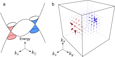
Figure 1: Nontrivial band structure and Berry curvature of a topological semimetal. (a) A schematic of the energy spectrum of a topological semimetal. $(k_{x},k_{y},k_{z})$ is the wave vector. $k_{||}^{2}=k_{x}^{2}+k_{y}^{2}$. (b) The vector plot of the Berry curvature in momentum space. The conduction and valence bands of a topological semimetal touch at the Weyl nodes, at which a pair of monopoles are hosted. The arrows show that the flux of the Berry curvature flows from one monopole (red) to the other (blue), defining the nontrivial topological properties of a topological semimetal. Adapted from Ref. Li et al. (2016b).

II Effective models

II.1 Two-node model of Weyl semimetal

A minimal model for a Weyl semimetal can be written as

$$H=A(k_{x}\sigma_{x}+k_{y}\sigma_{y})+\mathcal{M_{\mathbf{k}}}\sigma_{z},$$ (1)

where $\sigma$ are the Pauli matrices, $\mathcal{M}_{\mathbf{k}}=M_{0}-M_{1}(k_{x}^{2}+k_{y}^{2}+k_{z}^{2})$, $\mathbf{k}=(k_{x},k_{y},k_{z})$ is the wave vector, and $A$, $M_{0/1}$ are model parameters. This minimal model gives a global description of a pair of Weyl nodes of opposite chirality and all the topological properties. It has an identical structure as that for A-phase of ³He superfluids Shen (2012). If $M_{0}M_{1}>0$, the two bands intersect at $(0,0,\pm k_{w})$ with $k_{w}\equiv\sqrt{M_{0}/M_{1}}$ (see Fig. 1), giving rise to the topological semimetal phase. In the topological semimetal phase, the model can also be written as

$$H=A(k_{x}\sigma_{x}+k_{y}\sigma_{y})+M(k_{w}^{2}-\mathbf{k}^{2})\sigma_{z},$$ (2)

where $A$, $M$, $k_{w}$ are model parameters. The dispersions of two energy bands of this model are

$$E_{\pm}=\pm\sqrt{[M(k_{w}^{2}-\mathbf{k}^{2})]^{2}+A^{2}(k_{x}^{2}+k_{y}^{2})},$$ (3)

which reduce to $E_{\pm}=\pm M|k_{w}^{2}-k_{z}^{2}|$ at $k_{x}=k_{y}=0$. The two bands intersect at $(0,0,\pm k_{w})$ (see Fig. 1).

Around the two nodes $(0,0,\pm k_{w})$, $H$ reduces to two separate local models

$$H_{\pm}=\mathbf{M}_{\pm}\cdot\sigma,$$ (4)

$H_{\pm}=\mathbf{M}_{\pm}\cdot\sigma$with $\mathbf{M}_{\pm}=\left(A\widetilde{k}_{x},A\widetilde{k}_{y},\mp 2Mk_{w}\widetilde{k}_{z}\right)$ and $(\widetilde{k}_{x},\widetilde{k}_{y},\widetilde{k}_{z})$ the effective wave vector measured from the Weyl nodes.

II.2 Berry curvature

The topological properties in $H$ can be seen from the Berry curvature Xiao et al. (2010), $\Omega(\mathbf{k})$ = $\nabla_{\mathbf{k}}\times\mathbf{A}(\mathbf{k})$, where the Berry connection is defined as $\mathbf{A}(\mathbf{k})$ = $i\left\langle u(\mathbf{k})\right|\nabla_{\mathbf{k}}\left|u(\mathbf{k})\right\rangle$. For example, for the energy eigenstates for the $+$ band $\left|u(\mathbf{k})\right\rangle$ = $[\cos(\Theta/2),\sin(\Theta/2)e^{i\varphi}]$, where $\cos\Theta\equiv\mathcal{M}_{\mathbf{k}}/E_{+}$ and $\tan\varphi\equiv k_{y}/k_{x}$. The three-dimensional Berry curvature for the two-node model can be expressed as

$$\boldsymbol{\Omega}\left(\mathbf{k}\right)=\frac{A^{2}M}{E_{+}^{3}}\left[k_{z}k_{x},k_{z}k_{y},\frac{1}{2}\left(k_{z}^{2}-k_{w}^{2}-k_{x}^{2}-k_{y}^{2}\right)\right].$$

There exist a pair of singularities at $(0,0,\pm k_{w})$ as shown in Fig. 1. The chirality of a Weyl node can be found as an integral over the Fermi surface enclosing one Weyl node $(1/2\pi)\oint\Omega(\mathbf{k})\cdot d\mathbf{S(\mathbf{k})}$, which yields opposite topological charges $\mp\mathrm{sgn}(M)$ at $\pm k_{w}$, corresponding to a pair of “magnetic monopole and antimonopole” in momentum space.

II.3 $k_{z}$-dependent Chern number

For a given $k_{z}$, a Chern number can be well defined as $n_{c}(k_{z})=-(1/2\pi)\iint dk_{x}dk_{y}\Omega(\mathbf{k})\cdot\hat{z}$ to characterize the topological property in the $k_{x}$-$k_{y}$ plane, and Lu et al. (2010)

$$n_{c}(k_{z})=-\frac{1}{2}[\mathrm{sgn}[M(k_{w}^{2}-k_{z}^{2})]+\mathrm{sgn}(M)].$$ (6)

The Chern number $n_{c}(k_{z})=-\mathrm{sgn}(M)$ for $-k_{w}<k_{z}<k_{w}$, and $n_{c}(k_{z})=0$ otherwise Yang et al. (2011). The nonzero Chern number corresponds to the $k_{z}$-dependent edge states (known as the Fermi arcs) according to the bulk-boundary correspondence Hatsugai (1993).

II.4 Fermi arcs

If there is an open boundary at $y=0$, where the wave function vanishes, the dispersion of the surface states is finally given by Shen (2012); Zhang et al. (2016b)

$$E_{\text{arc}}(k_{x},k_{z})=\mathrm{sgn}(M)Ak_{x}.$$ (7)

The corresponding wavefunction is similar to that of topological insulator surface states Shan et al. (2010); Shen et al. (2011)

$$\Psi_{k_{x},k_{z}}^{\text{arc}}(\mathbf{r}) = Ce^{ik_{x}x+ik_{z}z}\begin{bmatrix}\text{sgn}(M)\\ 1\end{bmatrix}(e^{\lambda_{1}y}-e^{\lambda_{2}y}),$$ (8)

where $C$ is a normalization factor and $\lambda_{1,2}=A/2|M|\mp\sqrt{(A/2M)^{2}-\Delta_{k}}$, and $\Delta_{k}=k_{w}^{2}-k_{x}^{2}-k_{z}^{2}$. There are Fermi arcs in two cases: (i) $\lambda_{1,2}>0$, and (ii) $\lambda_{1,2}=a\mp ib$ with $a,b>0$ (Note that $\lambda_{1}=\lambda_{2}$ corresponds to a trivial case). Also in both cases (i) and (ii), we have $\lambda_{1}\lambda_{2}>0$ and henceforth $\Delta_{k}>0$. Therefore the solution of Fermi surface states is restricted inside a circle defined by $k_{x}^{2}+k_{z}^{2}<k_{w}^{2}$.

The two-node model in Eq. (2) provides a generic description for Weyl semimetals, including the band touching, opposite chirality, monopoles of Berry curvature, topological charges, and Fermi arcs.

II.5 Monopole charge

As an example, we use the effective model

$$H = vk\cdot\sigma$$ (9)

to demonstrate the monopole charge hosted at the Weyl nodes. The model is equivalent to Eq. (4). The spinor wave function of the valence band can be found as

$$|u_{+}(k,\theta,\varphi)\rangle = \left(\begin{array}[]{c}\sin\frac{\theta}{2}\\ -\cos\frac{\theta}{2}e^{i\varphi}\\ \end{array}\right),$$ (12)

where $\cos\theta\equiv k_{z}/k$ with $k=\sqrt{k_{x}^{2}+k_{y}^{2}+k_{z}^{2}}$. The Berry connection is defined as

$$\mathbf{A} \equiv -i\langle u_{+}\left|\nabla_{\mathbf{k}}\right|u_{+}\rangle.$$ (13)

In polar coordinates, $\nabla_{\mathbf{k}}=(\partial_{k},(1/k)\partial_{\theta},(1/k\sin\theta)\partial_{\varphi})$, we can find that

$$(A_{k},A_{\theta},A_{\varphi}) = (0,0,\frac{\cos^{2}\frac{\theta}{2}}{k\sin\theta}).$$ (14)

The Berry curvature can be found as

$$\mathbf{\Omega} \equiv \nabla\times\mathbf{A}$$ (15)

$$= \frac{1}{k\sin\theta}\left[\frac{\partial(A_{\varphi}\sin\theta)}{\partial\theta}\right]\hat{e}_{k}-\frac{1}{k}\frac{\partial(kA_{\varphi})}{\partial k}\hat{e}_{\theta}$$

$$= -\frac{1}{2k^{2}}\hat{e}_{k}.$$

The monopole charge is defind as the Berry curvature flux threading a sphere that encloses the origin, and can be found as

$$\mathcal{N} = \frac{1}{2\pi}\int_{\Sigma}d\mathbf{S}\cdot\mathbf{\Omega}$$ (16)

$$= \int_{0}^{2\pi}d\varphi\int_{0}^{\pi}d\theta\sin\theta k^{2}(-\frac{1}{2k^{2}})$$

$$= -1.$$

In the other valley of opposite chirality, the Hamiltonian can be written as $H=-vk\cdot\sigma$, the wave function of the valence band $|u_{-}\rangle$ can be obtained by letting $\theta\rightarrow\pi/2-\theta$ and $\varphi\rightarrow\pi+\varphi$ in $|u_{+}\rangle$, and $|u_{-}\rangle=(\cos\frac{\theta}{2},\sin\frac{\theta}{2}e^{i\varphi})$. Following the same procedure, we can show that the Berry connection is $A_{\varphi}=\sin^{2}\frac{\theta}{2}/k\sin\theta$, the Berry curvature is $\Omega_{k}=1/2k^{2}$, and the monopole charge is 1. Thus the total monopole charge is zero for the two-node model, which is consistent with Nielsen-Minomiya’s no-go theorem Nielsen and Ninomiya (1981).

II.6 Landau bands

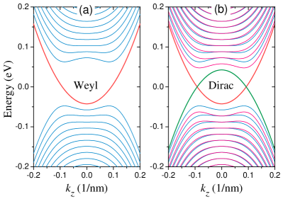
Figure 2: The energies of Landau bands of the minimal global model for Weyl and Dirac semimetals in a magnetic field $B$ applied along the $z$ direction, as functions of the wave vector $k_{z}$. The parameters: $M_{0}=0.05$ eV, $M_{1}=5$ eV$\cdot$nm², $A=1$ eV$\cdot$nm, and $B=1$ Tesla. The Zeeman energy is not included. Adapted from Lu et al. (2015).

In a magnetic field along the $z$ direction, the energy spectrum is quantized into a set of 1D Landau bands dispersing with $k_{z}$ [see Fig. 2 (a)]. We consider a magnetic field applied along the $z$ direction, $\mathbf{B}=(0,0,B)$, and choose the Landau gauge in which the vector potential is $\mathbf{A}=(-yB,0,0)$. The Landau bands can be solved analytically Shen et al. (2004, 2005); Sakurai (1993).

The eigen energies are Lu et al. (2015)

$$E_{k_{z}}^{\nu\pm} = \omega/2\pm\sqrt{\mathcal{M}_{\nu}^{2}+\nu\eta^{2}},\ \nu\geq 1$$

$$E_{k_{z}}^{0} = \omega/2-M_{0}+M_{1}k_{z}^{2},\ \ \nu=0,$$ (17)

where $\omega=2M/\ell_{B}^{2}$, $\eta=\sqrt{2}A/\ell_{B}$, and the magnetic length $\ell_{B}=\sqrt{\hbar/e|B|}$. The Landau energy bands ($\nu$ as band index) disperse with $k_{z}$, as shown in Fig. 2. The eigen states for $\nu\geq 1$ are

$$|\nu\geq 1,k_{x},k_{z},+\rangle = \left[\begin{array}[]{cc}\cos\frac{\theta_{k_{z}}^{\nu}}{2}|\nu-1\rangle\\ \sin\frac{\theta_{k_{z}}^{\nu}}{2}|\nu\rangle\end{array}\right]|k_{x},k_{z}\rangle,$$ (20)

$$|\nu\geq 1,k_{x},k_{z},-\rangle = \left[\begin{array}[]{cc}\sin\frac{\theta_{k_{z}}^{\nu}}{2}|\nu-1\rangle\\ -\cos\frac{\theta_{k_{z}}^{\nu}}{2}|\nu\rangle\end{array}\right]|k_{x},k_{z}\rangle,$$ (23)

and for $\nu=0$ is

$$|\nu=0,k_{x},k_{z}\rangle=\left[\begin{array}[]{cc}0\\ |0\rangle\end{array}\right]|k_{x},k_{z}\rangle,$$ (24)

where $\cos\theta^{\nu}_{k_{z}}=\mathcal{M}_{\nu}/\sqrt{\mathcal{M}_{\nu}^{2}+\nu\eta^{2}}$, and the wave functions $\psi_{\nu,k_{z},k_{x}}(\mathbf{r})=\langle\mathbf{r}|\nu,k_{x},k_{z}\rangle$ are found as

$$\psi_{\nu,k_{z},k_{x}}(\mathbf{r}) = \frac{C_{\nu}}{\sqrt{L_{x}L_{z}\ell_{B}}}e^{ik_{z}z}e^{ik_{x}x}e^{-\frac{(y-y_{0})^{2}}{2\ell_{B}^{2}}}\mathcal{H}_{\nu}(\frac{y-y_{0}}{\ell_{B}}),$$

where $C_{\nu}\equiv 1/\sqrt{\nu!2^{\nu}\sqrt{\pi}}$, $L_{x}L_{z}$ is area of sample, the guiding center $y_{0}=k_{x}\ell_{B}^{2}$, $\mathcal{H}_{\nu}$ are the Hermite polynomials. As the dispersions are not explicit functions of $k_{x}$, the number of different $k_{x}$ represents the Landau degeneracy $N_{L}=1/2\pi\ell_{B}^{2}=eB/h$ in a unit area in the x-y plane. This set of analytical solutions provides us a good base to study the transport properties of Weyl fermions.

II.7 Paramagnetic topological semimetals

A Weyl semimetal and its time-reversal partner can form a Dirac semimetal or paramagnetic semimetal, whose model can be built by $H(\mathbf{k})$ in Eq. (2) and its time-reversal partner $H^{*}(-\mathbf{k})$, where the asterisk refers to a complex conjugate. This model can also serve as a building block for Weyl semimetals that respect time-reversal symmetry but break inversion symmetry Huang et al. (2015a); Weng et al. (2015); Lv et al. (2015); Xu et al. (2015b); Yang et al. (2015c); Zhang et al. (2016a); Huang et al. (2015b); Xu et al. (2015c, 2016). For this case, there is the quantum spin Hall effect, compared to the quantum anomalous Hall effect in a Weyl semimetal of a single pair of nodes. A straightforward extension is as follows Zhang et al. (2016b)

$$H_{\text{Dirac}}=A(k_{x}\alpha_{x}+k_{y}\alpha_{y})+M(k_{w}^{2}-k^{2})\beta,$$ (26)

where the Dirac matrices are $\alpha_{x}=\sigma_{x}\otimes\sigma_{x}$, $\alpha_{y}=\sigma_{x}\otimes\sigma_{y}$, $\beta=\sigma_{z}\otimes\sigma_{0}$. It contains four Weyl nodes, which are doubly degenerate. The surface electrons around the $\hat{\mathbf{z}}$ direction consist of two branches with opposite spins and opposite effective velocities. The model can also be written into a block-diagonalized form by changing the basis ($1\rightarrow 1$, $4\rightarrow 2$, $2\rightarrow 3$, $3\rightarrow 4$),

$$H_{\text{Dirac}}=\left[\begin{array}[]{cc}H(\mathbf{k})&0\\ 0&H^{*}(-\mathbf{k})\end{array}\right]+\sigma_{z}\otimes\left[\begin{array}[]{cc}\Delta_{s}&0\\ 0&\Delta_{p}\end{array}\right].$$ (27)

In the second term, the $z$-direction Zeeman energy $\Delta_{s/p}=g_{s/p}\mu_{B}B/2$ is also included, where $g_{s/p}$ is the g-factor for the $s/p$ orbital Wang et al. (2013) and $\mu_{B}$ is the Bohr magneton.

Figure 2 (b) shows the Landau bands of both $H(\mathbf{k})$ and $H^{*}(-\mathbf{k})$ in the $z$-direction magnetic field. The Landau bands of the Dirac semimetal can be found in a similar way as that in Sec. II.6. Now there are two branches of $\nu=0$ bands, with the energy dispersions $E_{k_{z}}^{0\uparrow}=\omega/2+\Delta_{p}-M_{0}+M_{1}k_{z}^{2}$ and $E_{k_{z}}^{0\downarrow}=-\omega/2-\Delta_{s}+M_{0}-M_{1}k_{z}^{2}$ for $H(\mathbf{k})$ and $H^{*}(-\mathbf{k})$, respectively. They intersect at $k_{z}=\pm\sqrt{[M_{0}-(\omega+\Delta_{s}+\Delta_{p})/2]/M_{1}}$ and energy $(\Delta_{p}-\Delta_{s})/2$, and with opposite Fermi velocities near the points.

II.8 Double-Weyl semimetal

Each Weyl node in a Weyl semimetal hosts a monopole charge of 1 or -1. In a doulbe-Weyl semimetal, the monopole charge is 2 or -2 Xu et al. (2011); Fang et al. (2012); Guan et al. (2015); Huang et al. (2016). For a single valley of both single- and double-Weyl semimetals, the minimal model can be written as

$$H=\left[\begin{array}[]{cc}\chi v_{z}\hbar k_{z}&v_{\|}(\hbar k_{+})^{\mathcal{N}}\\ v_{\|}(\hbar k_{-})^{\mathcal{N}}&-\chi v_{z}\hbar k_{z}\\ \end{array}\right],$$ (28)

where $k_{\pm}=k_{x}\pm ik_{y}$, $\chi=\pm 1$ is the valley index, $v_{z}$ and $v_{||}$ are parameters and assumed to be constants, and momentum $\mathbf{k}$ is measured from the Weyl nodes. Here, $\mathcal{N}=1,2$ correspond to single- and double-Weyl semimetal respectively. The model has a conduction band and a valence band, with the dispersions given by $\pm E_{\mathbf{k}}$ and $E_{\mathbf{k}}=\sqrt{v_{z}^{2}\hbar^{2}k_{z}^{2}+v_{||}^{2}(\hbar^{2}k_{x}^{2}+\hbar^{2}k_{y}^{2})^{\mathcal{N}}}$. Without loss of generality, we assume that the chemical potential is slightly above the Weyl nodes and the electronic transport is contributed mainly by the conduction bands throughout the paper. The eigenstate of the conduction band at valley $\chi=+$ is given by

$$|\mathbf{k}\rangle=\left[\begin{array}[]{c}\cos(\theta/2)\\ \sin(\theta/2)\exp(-i\mathcal{N}\varphi)\\ \end{array}\right],$$ (31)

where $\cos\theta\equiv v_{z}k_{z}/E_{\mathbf{k}}$, and $\tan\varphi\equiv k_{y}/k_{x}$. The eigenstate of the conduction band around valley $\chi=-$ can be found by replacing $\cos(\theta/2)\rightarrow\sin(\theta/2)$ and $\sin(\theta/2)\rightarrow-\cos(\theta/2)$ in Eq. (31). The monopole charge can be found by integrating the Berry curvature over an arbitrary Fermi sphere $\Sigma$ that encloses the Weyl node,

$$\frac{1}{2\pi}\int_{\Sigma}d\mathbf{S}\cdot\mathbf{\Omega}=\pm\mathcal{N},$$ (32)

with $\pm$ for the $\pm$ valleys, the Berry curvature Xiao et al. (2010) $\mathbf{\Omega}=\nabla\times\mathbf{A}$, and $\mathbf{A}=(A_{\theta},A_{\varphi})$ is the Berry connection given by $A_{\theta}=\langle\mathbf{k}|i\partial_{\theta}|\mathbf{k}\rangle=0$ and $A_{\varphi}=\langle\mathbf{k}|i\partial_{\varphi}|\mathbf{k}\rangle=\mathcal{N}\sin^{2}(\theta/2)$.

III Near zero field: Weak anti-localization

Weak anti-localization is a transport phenomenon in disordered metals Lee and Ramakrishnan (1985). At low temperatures, when the mean free path is much shorter than the system size and phase coherence length, electrons suffer from scattering but can maintain their phase coherence. In this quantum diffusive regime, the quantum interference between time-reversed scattering loops can give rise to a correction to the conductivity. If the quantum interference correction is positive, it gives a weak anti-localization correction to the conductivity. Because this correction requires time reversal symmetry, it can be suppressed by applying a magnetic field, leading to a negative magnetoconductivity, or positive magnetoresistivity, as the signature for the weak anti-localization. The weak anti-localization has been widely observed in topological topological semimetals, including Bi_0.97Sb_0.03 ,Kim et al. (2013, 2014) ZrTe₅,Li et al. (2016a), Na₃Bi Xiong et al. (2015), Cd₃As₂ Li et al. (2015, 2016b), TaAs Huang et al. (2015b); Zhang et al. (2016a), etc.

III.1 Symmetry argument

In contrast, the quantum interference can be negative, leading to the weak localization effect and totally opposite temperate and magnetic dependencies of conductivity. Whether one has weak localization or weak anti-localization depends on the symmetry (see Table 1). According to the classification of the ensembles of random matrix Dyson (1962), there are three symmetry classes. If a system has time-reversal symmetry but no spin-rotational symmetry, it is in the symplectic class, in which the weak anti-localization is expected Hikami et al. (1980). Remember that one of the low-energy descriptions of Weyl fermions in semimetals is $H=\pm\hbar v_{F}\boldsymbol{\sigma}\cdot\mathbf{k}$, which respects time-reversal symmetry not spin rotational symmetry. Therefore, a single valley of Weyl fermions has the symplectic symmetry and the weak anti-localization. Moreover, we find the Berry phase can also explain the weak localization in Weyl semimetals Dai et al. (2016), which we discuss later.

Table 1: The relation between the symmetry classes (orthogonal, symplectic, and unitary) Dyson (1962) and weak localization (WL) and anti-localization (WAL) Hikami et al. (1980). Adapted from Ref. Lu and Shen (2016).

	Orthogonal	Symplectic	Unitary
Time-reversal	$\surd$	$\surd$	$\times$
Spin-rotational	$\surd$	$\times$	$\times$
WL/WAL	WL	WAL	$\times$

III.2 Feynman diagram calculations

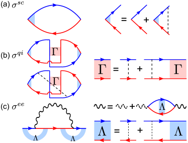
Figure 3: The Feynman diagrams McCann et al. (2006); Altshuler et al. (1980); Fukuyama (1980); Lee and Ramakrishnan (1985); Lu et al. (2011); Shan et al. (2012); Lu and Shen (2014b) for the conductivity of 3D Weyl semimetals, in the presence of disorder (dashed lines) and electron-electron interaction (wavy lines). The arrow lines are for Green’s functions. Adapted from Ref. Lu and Shen (2015).

One of the theoretical approaches to study the weak localization and anti-localization is the Feynman diagram techniques. Figure 3 summarizes the Feynman diagrams used to study the weak localization and anti-localization arising from the quantum interference and interaction Lu and Shen (2015). It is based on the linear response theory of the conductivity, with disorder and interaction taken as perturbations. In the formulism, there are three main contributions to the conductivity. The leading order is the semiclassical Drude conductivity [Fig. 3(a)], then the quantum interference correction [Fig. 3(b)] and interaction correction (Altshuler-Aronov effect) [Fig. 3(d)].

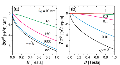
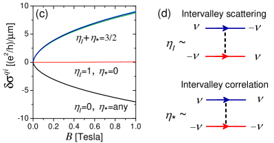
Figure 4: The magnetoconductivity $\delta\sigma^{qi}(B)$ for different phase coherence length $\ell_{\phi}$ at $\eta_{I}=\eta_{*}=0$ (a), for different $\eta_{I}$ at $\eta_{*}=0$ (b), and for different $\eta_{I}$ at finite $\eta_{*}$ (c). The magnetic field $B$ is applied along arbitrary directions. Parameters: $\ell=10$ nm and $\ell_{\phi}=1000$ nm in (b) and (c). (d) The diagrams show the difference between $\eta_{I}$ and $\eta_{*}$, with $\eta_{I}$ related to the intervalley scattering and $\eta_{*}$ measuring the intervalley correlation of intravalley scattering. The dashed lines represent the correlation of two scattering processes. $\nu=\pm$ is the valley index. Adapted from Ref. Lu and Shen (2015).

We calculate the magnetoconductivity arising from the quantum interference $\delta\sigma^{qi}$, as shown in Fig. 4. As $B\rightarrow 0$, $\delta\sigma^{qi}$ is proportional to $-\sqrt{B}$ for $\ell_{\phi}\gg\ell_{B}$ or at low temperatures, and $\delta\sigma^{qi}\propto-B^{2}$ for $\ell_{\phi}\ll\ell_{B}$ or at high temperatures. $\ell_{B}$ can be evaluated approximately as 12.8 nm$/\sqrt{B}$ with $B$ in Tesla. Usually below the liquid helium temperature, $\ell_{\phi}$ can be as long as hundreds of nanometers to one micrometer, much longer than $\ell_{B}$ which is tens of nanometers between 0.1 and 1 Tesla. Therefore, the $-\sqrt{B}$ magnetoconductivity at low temperatures and small fields serves as a signature for the weak anti-localization of 3D Weyl fermions. Fig. 4(a) shows $\delta\sigma^{qi}(B)$ of two valleys of Weyl fermions in the absence of intervalley scattering. For long $\ell_{\phi}$, $\delta\sigma^{qi}(B)$ is negative and proportional to $\sqrt{B}$, showing the signature of the weak anti-localization of 3D Weyl fermions. This $-\sqrt{B}$ dependence agrees well with the experiment,Kim et al. (2013, 2014) and we emphasize that it is obtained from a complete diagram calculation with only two parameters $\ell$ and $\ell_{\phi}$ of physical meanings. As $\ell_{\phi}$ becomes shorter, a change from $-\sqrt{B}$ to $-B^{2}$ is evident, and eventually $\delta^{qi}(B)$ vanishes at $\ell_{\phi}=\ell$ as the system is no longer in the quantum interference regime and enters the semiclassical diffusion regime.

III.3 Weak localization of double-Weyl semimetal

We focus on the Fermi sphere in one valley of a topological semimetal. For each path [labelled as $P$ in Fig. 5(a)] connecting successive intermediate states of the backscattering from $\mathbf{k}$ to $-\mathbf{k}$ on the Fermi sphere, which encompasses the monopole charge at the origin, there exists a corresponding time-reversal counterpart $P^{\prime}$. The quantum interference is determined by the phase difference between the two time-reversed paths $P$ and $P^{\prime}$, which is equivalent to the Berry phase accumulated along the loop formed by $P$ together with $\bar{P}\equiv-P^{\prime}$, namely the corresponding path from $-\mathbf{k}$ to $\mathbf{k}$, as shown in Fig. 5(b).

The quantum interference correction then depends on the geometric phase, i.e., the Berry phase Xiao et al. (2010); Pancharatnam (1956); Berry (1984); Shon and Ando (1998); Suzuura and Ando (2002); McCann et al. (2006), collected by electrons after circulating the loop $\mathcal{C}\equiv P+\bar{P}$. The Berry phase can be found by a loop integral of the Berry connection around $\mathcal{C}$. Remarkably, this Berry phase depends only on the monopole charge, but not on the specific shape of the loop Dai et al. (2016)

$$\gamma=\oint_{\mathcal{C}}d\mathbf{\ell}\cdot\mathbf{A}=\pi\mathcal{N}.$$ (33)

For double-Weyl semimetals, the monopole charge $\mathcal{N}=2$ and the Berry phase is then $2\pi$. With the $2\pi$ Berry phase, the time-reversed scattering loops interfere constructively, leading to the weak localization effect. However, for single-Weyl semimetals, the monopole charge is $\mathcal{N}=1$ and the Berry phase is $\pi$, which gives rise to the weak anti-localization effect. As the Berry phase is a consequence of the Berry curvature field generated by the monopole charge, we therefore establish a robust connection between the weak (anti)localization effect with the parity of monopole charge $\mathcal{N}$. The Berry phase argument is consistent with the symmetry classificationAltland and Zirnbauer (1997), the single-Weyl semimetals belong to the symplectic class with a weak anti-localization correction, while double-Weyl semimetals correspond to the orthogonal class with a weak localization correction.

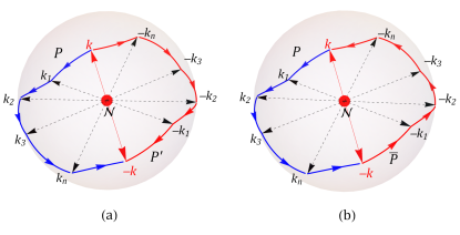
Figure 5: The Fermi sphere in momentum space for a three-dimensional topological semimetal, where the dot located at the origin represents a monopole charge of $\mathcal{N}$. (a) $P$ denotes a generic backscattering from the wave vector $\mathbf{k}$ to $-\mathbf{k}$ via intermediate states labeled as ($\mathbf{k}_{1},\mathbf{k}_{2},...,\mathbf{k}_{n}$). $P^{\prime}$ stands for the time-reversal counterpart of $P$. (b) The phase difference between $P$ and $P^{\prime}$ is equivalent to the Berry phase circulating around the loop $\mathcal{C}=P+\bar{P}$. Adapted from Ref. Dai et al. (2016).

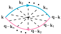
Figure 6: The maximally crossed Feynman diagram that describes the quantum interference between the time-reversed scattering trajectories in Fig. 5 as $\mathbf{q}\rightarrow 0$. The arrowed solid and dashed lines denote the Green functions and impurity scattering, respectively. This kind of diagrams can give the quantum interference correction to the conductivity Hikami et al. (1980); Shon and Ando (1998); McCann et al. (2006). A negative (positive) correction corresponds to the weak (anti)localization effect, with the sign sensitive to the parity of the monopole charge. Adapted from Ref. Dai et al. (2016).

We now verify the above argument of quantum interference correction to conductivity in Weyl semimetals by the standard Feynman diagram calculations. The correction can be evaluated by calculating the maximally crossed diagrams, one of which is shown in Fig. 6. In this diagram, the segments of the arrow lines represent the intermediate states in the backscattering, and the dashed lines represent the correlation between the time-reversed scattering processes. The core calculation of the maximally crossed diagrams can be formulated into the particle-particle correlation, known as the cooperon. The cooperon of the double-Weyl semimetal is found to be Dai et al. (2016)

$$\Gamma_{\mathbf{k}_{1},\mathbf{k}_{2}}\approx\frac{\hbar}{2\pi N_{F}\tau^{2}}\frac{e^{i2(\varphi_{2}-\varphi_{1})}}{D_{1}\left(q_{x}^{2}+q_{y}^{2}\right)+D_{2}q_{z}^{2}},$$ (34)

where $\mathbf{q}=\mathbf{k}_{1}+\mathbf{k}_{2}$ is the cooperon wave vector, $\mathbf{k}_{1}$ and $\mathbf{k}_{2}$ are the wave vectors of incoming and outgoing states, respectively, $\varphi_{1}$ and $\varphi_{2}$ are the azimuth angles of corresponding wave vectors, $D_{1}=8\tau E_{F}v_{\|}/3\pi$ and $D_{2}=\tau v_{z}^{2}$ are the diffusion coefficients, $N_{F}$ is the density of states, and $\tau$ is the transport time. In contrast, the cooperon of the single-Weyl semimetal is known to take the form Lu and Shen (2015)

$$\Gamma_{\mathbf{k}_{1},\mathbf{k}_{2}}\approx\frac{\hbar}{2\pi N_{F}\tau^{2}}\frac{1}{Dq^{2}}e^{i(\varphi_{2}-\varphi_{1})},$$ (35)

where the diffusion coefficient $D=v^{2}_{F}\tau/2$ (We only give the result for isotropic single-Weyl semimetals with $v_{F}=v_{z}=v_{\|}$; this simplification does not change any qualitative results with respect to quantum interference correction). Note the main difference between Eqs. (34) and (35) lies in the phase factor involving $\varphi_{2}-\varphi_{1}$, which originates from different eigenstates of Weyl semimetals with different monopole charges.

As $\mathbf{q}\to 0$, i.e., $\mathbf{k}_{1}=-\mathbf{k}_{2}$, the cooperon becomes divergent and becomes the most dominant contribution to the backscattering. In this limit, $\varphi_{2}=\varphi_{1}+\pi$ (We have carried out a coordinate transformation in deriving these results, where $\hbar k_{x}=\sqrt{k\sin\theta}\cos\varphi,\hbar k_{y}=\sqrt{k\sin\theta}\sin\varphi,2\hbar mvk_{z}=k\cos\theta$, $-\mathbf{k}$ is obtained by setting $\varphi\to\varphi+\pi$ and $\theta\to\pi-\theta$). Then, for the double-Weyl semimetal,

$$\Gamma_{\mathbf{k},\mathbf{q}-\mathbf{k}} \approx +\frac{\hbar}{2\pi N_{F}\tau^{2}}\frac{1}{D_{1}\left(q_{x}^{2}+q_{y}^{2}\right)+D_{2}q_{z}^{2}},$$ (36)

and for the single-Weyl semimetal,

$$\Gamma_{\mathbf{k},\mathbf{q}-\mathbf{k}} \approx -\frac{\hbar}{2\pi N_{F}\tau^{2}}\frac{1}{Dq^{2}}.$$ (37)

Note the different signs in Eqs. (36) and (37), which correspond to the WL and WAL effects, respectively. This is a direct consequence of different phase factors in the wavefunctions, generated by different monopole charges in double- and single-Weyl semimetals. In other words, a connection is therefore firmly established between the parity of monopole charge $\mathcal{N}$ and the sign of the quantum interference correction, with odd and even parity giving rise to WAL and WL, respectively.

The weak localization effect can give rise to a positive magnetoconductivity as another signature of the weak localization in double-Weyl semimetals. The magnetoconductivity is anisotropic, depending on whether the field is along the $z$ direction or in the $x-y$ plane. The magnetoconductivity is defined as $\delta\sigma^{\textrm{qi}}_{zz}(B)=\sigma^{\textrm{qi}}_{zz}(B)-\sigma^{\textrm{qi}}_{zz}(0)$. In the limit of $\ell_{\phi}\gg\ell_{B}\gg\ell_{z}$, which can be approached at low temperatures, the magnetoconductivity $\delta\sigma^{\textrm{qi}}_{zz}(B)\propto\sqrt{B}$. In the limit of $\ell_{B}\gg\ell_{\phi}$ and $\ell_{B}\gg\ell_{z}$, $\delta\sigma^{\textrm{qi}}_{zz}(B)\propto B^{2}$.

III.4 Magnetoconductivity formula for WAL/WL in 3D

Based on our theoretical results in Refs. Lu and Shen (2015) and Dai et al. (2016), we proposed a formula to fit the magnetoconductivity arising from the weak (anti-)localization in three dimensions,

$$\delta\sigma^{\textrm{qi}}_{zz} = C^{\textrm{qi}}_{1}\frac{B^{2}\sqrt{B}}{B_{c}^{2}+B^{2}}+C^{\textrm{qi}}_{2}\frac{B_{c}^{2}B^{2}}{B_{c}^{2}+B^{2}},$$ (38)

where the fitting parameters $C^{\textrm{qi}}_{1}$ and $C^{\textrm{qi}}_{2}$ are positive for weak localization and negative for weak anti-localization. The critical field $B_{c}$ is related to the phase coherence length $\ell_{\phi}$ according to $B_{c}\sim\hbar/e\ell_{\phi}^{2}$. Empirically, the phase coherence length becomes longer with decreasing temperature and can be written as $\ell_{\phi}\sim T^{-p/2}$; then $B_{c}\sim T^{p}$, where $p$ is positive and determined by decoherence mechanisms such as electron-electron interaction ($p=3/2$) or electron-phonon interaction ($p=3$). At high temperatures, $\ell_{\phi}\rightarrow 0$; thus, $B_{c}\rightarrow\infty$ and we have $\delta\sigma^{\textrm{qi}}_{zz}\propto B^{2}$. At low temperatures, $\ell_{\phi}\rightarrow\infty$; then $B_{c}=0$ and we have $\delta\sigma^{\textrm{qi}}_{zz}\propto\sqrt{B}$. The formula has been applied in the experiment on TaAs, and by fitting the magnetoconductivity, we find that $p\approx 1.5$ Zhang et al. (2016a).

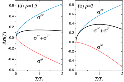
Figure 7: A schematic demonstration of the change of conductivity $\Delta\sigma$ as a function of temperature $T$. We choose $c_{ee}=c_{qi}$. $T_{c}$ is the critical temperature below which the conductivity drops with decreasing temperature. Adapted from Ref. Lu and Shen (2015).

III.5 Localization induced by interaction and inter-valley effects

In the presence of the interaction, we find that the change of conductivity with temperature for one valley of Weyl fermions can be summarized as

$$\Delta\sigma(T)=c_{ee}T^{1/2}-c_{qi}T^{p/2},$$ (39)

where both $c_{ee}$ and $c_{qi}$ are positive parameters. This describes a competition between the interaction-induced weak localization and interference-induced weak anti-localization, as shown in Fig. 7 schematically. At higher temperatures, the conductivity increases with decreasing temperature, showing a weak anti-localization behavior. Below a critical temperature $T_{c}$, the conductivity starts to drop with decreasing temperature, exhibiting a localization tendency. The critical temperature can be found as $T_{c}=\left(c_{ee}/p\cdot c_{qi}\right)^{2/(p-1)}$. Because $c_{ee},c_{qi}>0$, this means as long as $p>1$, there is always a critical temperature, below which the conductivity drops with decreasing temperature. For known decoherence mechanisms in 3D, $p$ is always greater than 1 Lee and Ramakrishnan (1985). With a set of typical parameters, we find that $T_{c}\approx 0.4\sim 10^{6}$ K Lu and Shen (2015).

We find that the intervalley scattering and correlation can also lead to the weak localization. Two dimensionless parameters are defined for the inter- and intravalley scattering: $\eta_{*}\propto\langle U_{\mathbf{k},\mathbf{k}^{\prime}}^{++}U_{\mathbf{k}^{\prime},\mathbf{k}}^{--}\rangle$ measuring the correlation between intravalley scattering and $\eta_{I}\propto\langle U_{\mathbf{k},\mathbf{k}^{\prime}}^{+-}U_{\mathbf{k}^{\prime},\mathbf{k}}^{-+}\rangle$ measuring the weight of intervalley scattering , where $U_{\mathbf{k},\mathbf{k}^{\prime}}^{\nu,\nu^{\prime}}$ is the scattering matrix element. Figure 4(d) schematically shows the difference between $\eta_{*}$ and $\eta_{I}$. As shown in Fig. 4(b), with increasing $\eta_{I}$, the negative $\delta\sigma^{qi}$ is suppressed, where $\eta_{I}\rightarrow 1$ means strong intervalley scattering while $\eta_{I}\rightarrow 0$ means vanishing intervalley scattering. Furthermore, Fig. 4(c) shows that the magnetoconductivity can turn to positive when $\eta_{I}+\eta_{*}=3/2$. The positive $\delta\sigma^{qi}(B)$ in Fig. 4(c) corresponds to a suppressed $\sigma^{qi}$ with decreasing temperature, i.e., a localization tendency. This localization is attributed to the strong intervalley coupling which recovers spin-rotational symmetry (now the spin space is complete for a given momentum), then the system goes to the orthogonal class Dyson (1962); Hikami et al. (1980); Suzuura and Ando (2002). Therefore, we show that the combination of strong intervalley scattering and correlation will strengthen the localization tendency in disordered Weyl semimetals. The metal-insulator phase transition is also found numerically Chen et al. (2015a).

IV Weak magnetic fields: Negative magnetoresistance

In a topological semimetal, paired Weyl nodes carry opposite chirality and paired monopoles and anti-monopoles of Berry curvature in momentum spaceVolovik (2003) [see 1(b)]. The nontrivial Berry curvature can couple an external magnetic field to the velocity of electrons, leading to a chiral current that is linearly proportional to the field. The correlation of chiral currents further contributes to an extra conductivity that quadratically grows with increasing magnetic field, in a magnetic field and an electric field applied parallel to each other Son and Spivak (2013); Burkov (2014). This $B^{2}$ positive conductivity in weak parallel magnetic fields, or negative magnetoresistance (negative MR), is rare in non-ferromagnetic materials, thus can serve as one of the transport signatures of the topological semimetals. More importantly, because of its relation to the chiral charge pumping between paired Weyl nodes, the negative magnetoresistance is also believed to be a signature of the chiral anomaly Adler (1969); Bell and Jackiw (1969); Nielsen and Ninomiya (1981). The negative magnetoresistance has been observed in topological insulator thin films Wang et al. (2012b) and many topological semimetals, including BiSb alloyKim et al. (2013, 2014), ZrTe₅ Li et al. (2016a), TaAs Zhang et al. (2016a); Huang et al. (2015b), Na₃Bi Xiong et al. (2015), Cd₃As₂ Li et al. (2015); Zhang et al. (2015a); Li et al. (2016b), TaP Arnold et al. (2016), NbAs Yang et al. (2015a, b), and HfTe₅ Wang et al. (2016c).

To understand the negative magnetoresistance, we start with the semiclassical equation of motion proposed by Niu and his colleagues Chang and Niu (1995); Sundaram and Niu (1999); Xiao et al. (2010); Zhou et al. (2013)

$$\mathbf{\dot{r}} = \mathbf{v}+\mathbf{\dot{k}}\times\mathbf{\Omega}_{\mathbf{k}}$$

$$\hbar\mathbf{\dot{k}} = e\mathbf{E}+e\mathbf{\dot{r}}\times\mathbf{B}$$ (40)

where $\mathbf{v}=\ \partial\epsilon_{\mathbf{k}}/\hbar\partial\mathbf{k}$. The second term in the first equation indicates that an electron can acquire an anomalous velocity proportional to the Berry curvature of the band in the presence of an electric field. This anomalous velocity is responsible for a number of transport phenomena.

Iterating $\mathbf{k}$ and $\mathbf{r}$ in the equations, using $(\mathbf{a}\times\mathbf{b})\times\mathbf{c}=(\mathbf{a}\cdot\mathbf{c})\mathbf{b}-(\mathbf{b}\cdot\mathbf{c})\mathbf{a}$, and $(\mathbf{\dot{a}}\times\mathbf{b})\cdot\mathbf{b}=0$, we arrive at Son and Spivak (2013)

$$\mathbf{\dot{r}} = \left(1+\frac{e}{\hbar}\mathbf{B}\cdot\mathbf{\Omega}_{\mathbf{k}}\right)^{-1}\left[\mathbf{v}+\frac{e}{\hbar}\mathbf{E}\times\mathbf{\Omega}_{\mathbf{k}}+\frac{e}{\hbar}(\mathbf{\Omega}_{\mathbf{k}}\cdot\mathbf{v})\mathbf{B}\right],$$

$$\hbar\mathbf{\dot{k}} = (1+\frac{1}{\hbar}\mathbf{B}\cdot\mathbf{\Omega}_{\mathbf{k}})^{-1}\left[e\mathbf{E}+e\mathbf{v}\times\mathbf{B}+\frac{e^{2}}{\hbar}(\mathbf{E}\cdot\mathbf{B})\mathbf{\Omega}_{\mathbf{k}}\right],$$

where $\mathbf{E}\times\mathbf{\Omega}_{\mathbf{k}}$ gives AHE Goswami and Tewari (2013); Zyuzin and Burkov (2012), $(\mathbf{\Omega}_{\mathbf{k}}\cdot\mathbf{v})\mathbf{B}$ gives the chiral magnetic effect Chang and Yang (2015), and $(\mathbf{E}\cdot\mathbf{B})\mathbf{\Omega}_{\mathbf{k}}$ is the source of the negative magnetoresistance Son and Spivak (2013); Burkov (2014).

Now we give an argument for the negative magnetoresistance. The argument is similar to the calculation by Yip Yip (2015). In the framework of linear response theory, $\mathbf{E}=0$, the velocity in small $B$ fields reduces to

$$\mathbf{\dot{r}} = \mathbf{v}+\frac{e}{\hbar}(\mathbf{\Omega}_{\mathbf{k}}\cdot\mathbf{v})\mathbf{B},$$ (42)

where we have considered the correction of the density of states by the Berry curvature. The second term represents the anomalous velocity induced by the finite Berry curvature and is proportional to the magnetic field. Because the conductivity is a current-current correlation [see Fig. 3(a)], the linear-$B$ dependence in the velocity (note that current is charge times velocity) leads to the quadratic-$B$ dependence in the conductivity. In Sec. II.5, we have shown that the Berry curvature is proportional to $1/k^{2}$. Considering there are $\Omega^{2}$ and a $k^{2}$ in the 3D integral of the conductivity formula, eventually, the anomalous conductivity part should be inversely proportional to the Fermi wave vector and proportional to $B^{2}$, that is

$$\delta\sigma(B)\propto\frac{B^{2}}{k_{F}^{2}}$$ (43)

The functional relation obtained by this argument is consistent with the formulas obtained by Son and Spivak Son and Spivak (2013) and Burkov Burkov (2014). The conductivity increases with $B^{2}$, giving rise to a negative magnetoresistance. Because the nontrivial Berry curvature diverges at the Weyl nodes, the positive conductivity will increase with decreasing Fermi wave vector and carrier density. In three dimensions, the carrier density $n$ is proportional to $k_{F}^{3}$, so

$$\delta\sigma(B)\propto\frac{B^{2}}{n^{2/3}}.$$ (44)

Therefore, it is necessary to check three properties in order to verify a negative magnetoresistance from the nontrivial Berry curvature. (i) The angular dependence. Because of the $\mathbf{E}\cdot\mathbf{B}$ term in Eq. (IV), the effect is maximized when the electric field is aligned with the magnetic field. Also, when the field is perpendicular to the current, the positive magnetoresistance from the Lorentz force can easily overwhelm the Berry-curvature negative magnetoresistance. (ii) The $B^{2}$ magnetic field dependence. (iii) The $n^{-2/3}$ carrier density dependence. So far, the first two properties have been verified by all the experiments in which the negative magnetoresistance is observed. In the experiment by Li et al. on a nanoribbon of Cd₃As₂ Li et al. (2016b), the carriers can be released by defects with increasing temperature, following an Arrhenius’s law. The carrier density was extracted from two formulas. One is Kohler’s rule $R(B_{\perp})=R_{0}[1+(\mu B_{\perp})^{2}]$, where $R(B_{\perp})$ and $R_{0}$ are the resistance in the presence and absence of a perpendicular magnetic field $B_{\perp}$, and $\mu$ is the mobility. This can give a rough estimate of the mobility $\mu$, which is then put into the zero-field resistivity $\rho=1/ne\mu$ to yield the carrier density $n$ approximately. In a temperature window between 50K and 150K, the weak anti-localization does not play a role, and the change in the negative magnetoresistance can be assumed to be mainly from the change of the carrier density because it is a semiclassical conductivity contribution. The experiment shows that the coefficient in front of the negative magnetoresistance can be well fitted by $B^{2}/n^{2/3}$. In the experiment by Zhang et al. Zhang et al. (2016a), the carrier density dependence was checked by comparing the results from different samples.

V Strong magnetic fields: the quantum limit

V.1 Argument of negative magnetoresistance in the quantum limit

According to Nielsen and Ninomiya Nielsen and Ninomiya (1983), the original proposal for realizing the chiral anomaly in lattices is in the quantum limit of a 3D semimetal. They started with a one-dimensional model in which two chiral energy bands have linear dispersions and opposite velocities. An external electric field can accelerate electrons in one band to higher energy levels, in this way, charges are “created”. In contrast, in the other band, which has the opposite velocity, charges are annihilated. The chiral charge, defined as the difference between the charges in the two bands, therefore is not conserved in the electric field. This is literally the chiral anomaly. As one of the possible realizations of the one-dimensional chiral system, they then proposed to use the $\nu=0$ Landau bands of a three-dimensional semimetal, and expected “the longitudinal magneto-conduction becomes extremely strong”. In other words, the magnetoresistance of the 0th Landau bands in semimetals is the first physical quantity that was proposed as one of the signatures of the chiral anomaly.

In the quantum limit, only the band of $\nu=0$ is partially filled. In this case the transport properties of the system are dominantly determined by the highly degenerate $\nu=0$ Landau bands [the red curve in Fig. 2 (a)]. It is reasonable to regard them as a bundle of one-dimensional chains. Combining the Landau degeneracy $N_{L}$, the $z$-direction conductance is approximately given by

$$\sigma_{zz}=N_{L}\sigma_{\text{1D}},$$ (45)

where $\sigma_{\text{1D}}$ is the conductance for each one-dimensional Landau band.

If we ignore the scattering between the states in the degenerate Landau bands, according to the transport theory, the ballistic conductance of a one-dimensional chain in the clean limit is given by

$$\sigma_{\text{1D}}=\frac{e^{2}}{h},$$ (46)

then the conductivity is found as

$$\sigma_{zz}=\frac{e^{2}}{h}\frac{eB}{h},$$ (47)

which is is linear in magnetic field $B$, giving a positive magnetoconductivity.

In most measurements, the sample size is much larger than the mean free path, then the scattering between the states in the Landau bands is inevitable, and we have to consider the other limit, i.e., the diffusive limit. Usually, the scattering is characterized by a momentum relaxation time $\tau$. According to the Einstein relation, the conductivity of each Landau band in the diffusive limit is

$$\sigma_{\text{1D}}=e^{2}N_{\text{1D}}v_{F}^{2}\tau,$$ (48)

where $v_{F}$ the Fermi velocity and the density of states for each 1D Landau band is $N_{\text{1D}}=1/\pi\hbar v_{F}$, then

$$\sigma_{zz}=\frac{e^{2}}{h}\frac{eBv_{F}\tau}{\pi\hbar}.$$ (49)

If $v_{F}$ and $\tau$ are constant, one readily concludes that the magnetoconductivity is positive and linear in $B$.

Recently, several theoretical works have formulated the negative magnetoresistance or positive magnetoconductivity in the quantum limit as one of the signatures of the chiral anomaly Son and Spivak (2013); Gorbar et al. (2014), much similar to those in Eqs. (47) and (49). In both cases, the positive magnetoconductivity arises because the Landau degeneracy increases linearly with $B$. However, in the following, we will show that if $v_{F}$ and $\tau$ also depend on the magnetic field, the conclusion has to be reexamined.

V.2 Disorder scattering

One of the convenient choices is the random Gaussian potential

$$U(\mathbf{r}) = \sum_{i}\frac{u_{i}}{(d\sqrt{2\pi})^{3}}e^{-|\mathbf{r}-\mathbf{R}_{i}|^{2}/2d^{2}},$$ (50)

where $u_{i}$ measures the scattering strength of a randomly distributed impurity at $\mathbf{R}_{i}$, and $d$ is a parameter that determines the range of the scattering potential. The Gaussian potential allows us to study the effect of the potential range in a controllable way, which we find it crucial in the present study. Now we have two characteristic lengths, the potential range $d$ and the magnetic length $\ell_{B}$, which define two regimes, the long-range potential regime $d\gg\ell_{B}$ and the short-range potential limit $d\ll\ell_{B}$. Note that, for a given $d$ in realistic materials, varying the magnetic field alone can cross between the two regimes. Empirically, the magnetic length $\ell_{B}$ = 25.6 nm /$\sqrt{|B|}$ with $B$ in Tesla. In the strong-field limit, e.g., $B>10$ T, the magnetic length $\ell_{B}$ becomes less than 10 nm, it is reasonable to regard smooth fluctuations in materials as long-range.

For the scattering among the states on the Fermi surface of the $0$th Landau bands, the transport time can be found as

$$\frac{\hbar}{\tau^{0,\text{tr}}_{k_{F}}} = 2\pi\sum_{k_{x}^{\prime},k_{z}^{\prime}}\langle|U^{0,0}_{k_{x},k_{F};k_{x}^{\prime},k_{z}^{\prime}}|^{2}\rangle\delta(E_{F}-E^{0}_{k_{z}^{\prime}})$$ (51)

$$\times(1-\frac{v^{z}_{0,k_{z}^{\prime}}}{v_{F}}),$$

where $U^{0,0}_{k_{x},k_{F};k_{x}^{\prime},k_{z}^{\prime}}$ represents the scattering matrix elements calculated from Eq. (50) and $\langle...\rangle$ means the impurity average Zhang et al. (2016b).

V.3 Negative magnetoconductivity with Delta potential

The delta potential means $d\rightarrow 0$ in Eq. (50). In this case, the transport time is the same as the scattering time Lu et al. (2015). By considering the magnetic field dependence of the scattering time, we find that in the strong-field limit ($B\rightarrow\infty$),

$$\tau = \frac{\hbar^{2}v_{F}^{0}\pi\ell_{B}^{2}}{V_{\text{imp}}}.$$ (52)

Here we suppress the correction $\Lambda$ , because it cancels in $\sigma_{zz}$ Lu et al. (2015). The scattering time can be put into Eq. (49) to give the conductivity in the strong-field limit as

$$\sigma_{zz,0}^{sc} = \frac{e^{2}}{h}\frac{(\hbar v_{F}^{0})^{2}}{V_{\text{imp}}}.$$ (53)

Notice that the Landau degeneracy in the scattering time cancels with that in Eq. (49), thus the magnetic field dependence of $\sigma_{zz,0}^{sc}$ is given by the Fermi velocity $v_{F}^{0}$. When ignoring the magnetic field dependence of the Fermi velocity, a $B$-independent conductivity was concluded, which is consistent with the previous work in which the velocity is constant Aji (2012). We find the magnetic field dependence of the Fermi velocity can lead to different scenarios of positive and negative magnetoconductivity.

(i) Weyl semimetal with fixed carrier density. In a strong field the Fermi velocity or the Fermi energy is given by the density of charge carriers and the magnetic field Abrikosov (1998). We assume that an ideal Weyl semimetal is the case that the Fermi energy crosses the Weyl nodes, all negative bands are fully filled and the positive bands are empty. In this case $\hbar v_{F}^{0}=2M_{1}k_{w}$. An extra doping of charge carriers will cause a change of electron density $n_{0}(>0)$ in the electron-doped case or hole density $n_{0}(<0)$ in the hole-doped case. The relation between the Fermi wave vector and the density of charge carriers is given by

$$n_{0}=2N_{L}\times\frac{k_{F}^{0}-k_{w}}{2\pi}$$ (54)

This means that the Fermi wave vector is determined by the density of charge carriers $n_{0}$ and magnetic field $B$,

$$k_{F}^{0} = k_{w}+\pi n_{0}h/eB$$ (55)

or $k_{F}^{0}=k_{w}+2\pi^{2}n_{0}\ell_{B}^{2}$. Thus the Fermi velocity is also a function of $B$, $\hbar v_{F}^{0}=2M_{1}k_{F}^{0},$ and

$$\sigma_{zz,0}^{sc}=\sigma_{N}\left[1+\mathrm{sgn}(n_{0})\frac{B_{c}}{B}\right]^{2}.$$ (56)

where the characteristic field $B_{c}=\pi\left|n_{0}\right|h/ek_{w}$. A typical order of $B_{c}$ is about 10 Tesla for $n_{0}$ of 10¹⁷/cm³. $\sigma_{zz,0}^{sc}$ is constant for the undoped case of $n_{0}=0$, and

$$\sigma_{N}=\frac{e^{2}}{h}\frac{4M_{1}^{2}k_{w}^{2}}{V_{\text{imp}}}$$ (57)

is the conductivity of the undoped case, and is independent of magnetic field. Thus the magnetoconductivity is always negative in the electron-doped case while always positive in the hole-doped regime.

(ii) Weyl semimetal with fixed Fermi energy. In the case that the Fermi energy is fixed, $(\hbar v_{F}^{0})^{2}=4M_{1}(E_{F}-eM_{1}B/\hbar+M_{0})$, and we have

$$\sigma_{zz,0}^{sc} = \frac{e^{2}}{h}\frac{4M_{1}(E_{F}-eM_{1}B/\hbar+M_{0})}{V_{\text{imp}}},$$ (58)

then the magnetoconductivity is always negative and linear in $B$.

(iii) Paramagnetic semimetal. For the Dirac semimetal or paramagnetic semimetal described by Eq. (27), there are two branches of $\nu=0$ bands, with the energy dispersions $E_{k_{z}}^{0\uparrow}=\omega/2+\Delta_{p}-M_{0}+M_{1}k_{z}^{2}$ and $E_{k_{z}}^{0\downarrow}=-\omega/2-\Delta_{s}+M_{0}-M_{1}k_{z}^{2}$ for $H(\mathbf{k})$ and $H^{*}(-\mathbf{k})$, respectively. In the absence of inter-block velocity, the longitudinal conductance along the $z$ direction is approximately a summation of those for two independent Weyl semimetals. First, we consider the Fermi energy cross both bands $0\uparrow$ and $0\downarrow$. Using Eq. (58), the $z$-direction conductivity is found as

$$\sigma_{zz,0}^{sc} = \sigma_{zz,0\uparrow}^{sc}+\sigma_{zz,0\downarrow}^{sc}$$ (59)

$$= \frac{e^{2}}{h}\frac{8M_{1}}{V_{\text{imp}}}[M_{0}-\frac{eM_{1}B}{\hbar}-\frac{\mu_{B}(g_{p}+g_{s})B}{4}],$$

or using $\sigma_{N}$ defined in Eq. (57),

$$\sigma_{zz,0}^{sc} = 2\sigma_{N}[1-\frac{eB}{\hbar k_{w}^{2}}-\frac{\mu_{B}(g_{p}+g_{s})B}{4M_{0}}].$$ (60)

In this case we have a negative linear $B$ magnetoconductivity, when the Fermi energy crosses both $E_{k_{z}}^{0\uparrow}$ and $E_{k_{z}}^{0\downarrow}$. With increasing magnetic field, the $0\uparrow$ bands will shift upwards and the $0\downarrow$ bands will shift downwards. Beyond a critical field, the Fermi energy will fall into either $0\uparrow$ or $0\downarrow$ bands, depending on whether the carriers are electron-type or hole-type. If the carrier density is fixed, the Fermi wave vector in this case does not depend on $k_{w}$ as that in Eq. (55), but

$$k_{F}^{0} = \frac{\pi n_{0}h}{eB}$$ (61)

or $k_{F}^{0}=2\pi^{2}n_{0}\ell_{B}^{2}$. In this case, with increasing magnetic field, the Fermi energy will approach the band edge and the Fermi velocity always decreases. Using Eq. (53),

$$\sigma_{zz,0}^{sc} = \frac{e^{2}}{h}\frac{4\pi^{2}h^{2}M_{1}^{2}n_{0}^{2}}{V_{\text{imp}}e^{2}B^{2}},$$ (62)

which also gives negative magnetoconductivity that is independent on the type of carriers. Note that in the Weyl semimetal TaAs with broken inversion symmetry, where the Weyl nodes always come in even pairs because of time-reversal symmetry Weng et al. (2015); Huang et al. (2015a); Lv et al. (2015); Xu et al. (2015b), the situation is more similar to that for the Dirac semimetal and the magnetoconductivity does not depend on the type of carriers and may be described by a generalized version of Eqs. (60) and (62).

V.4 Positive linear magnetoconductivity and zero-field minimum conductivity at half filling of a Weyl semimetal

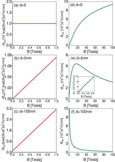
Figure 8: The longitudinal conductivity $\sigma_{zz}$ and transverse conductivity $\sigma_{xx}$ of the Weyl semimetal in the $\hat{\bf{z}}$-direction magnetic field $B$ for different potential ranges. The shared parameters: $k_{w}=0.1$/nm, $M=5$ eV$\cdot$nm², $A=1$ eV$\cdot$nm, $V_{\text{imp}}=10$ (eV)²$\cdot$nm³. Adapted from Ref. Zhang et al. (2016b).

With the random Gaussian potential, we can find the transport time as well as the conductivity. In particular, at the Weyl nodes the transport time is obtained as Zhang et al. (2016b)

$$\frac{\hbar}{\tau^{0,\text{tr}}_{k_{w}}} = \frac{V_{\text{imp}}}{2\pi Mk_{w}}\frac{e^{-4d^{2}k_{w}^{2}}}{2d^{2}+\ell_{B}^{2}},$$ (63)

and hence the longitudinal conductivity

$$\sigma_{zz}(B) = \frac{e^{2}}{h}\frac{(2Mk_{w})^{2}(2d^{2}+\ell_{B}^{2})}{V_{\text{imp}}\ell_{B}^{2}}e^{4d^{2}k_{w}^{2}},$$ (64)

where $V_{\text{imp}}\equiv\sum_{i}u_{i}^{2}/V$ measures the strength of the scattering and $V=L_{x}L_{y}L_{z}$ is the volume of the system. $L_{x,y,z}$ are the sizes of the system along the $\hat{\mathbf{x}}$, $\hat{\mathbf{y}}$ and $\hat{\mathbf{z}}$ directions, respectively. This conductivity is generated by the inter-node scattering with a momentum transfer of $2k_{w}$. As the magnetic field goes to zero, the magnetic length diverges and $d/\ell_{B}\rightarrow 0$, and Eq. (64) gives a minimum conductivity

$$\sigma_{zz}(0) = \frac{e^{2}}{h}\frac{4(Mk_{w})^{2}}{V_{\text{imp}}}e^{4d^{2}k_{w}^{2}},$$ (65)

even though the DOS vanishes at the Weyl nodes at zero magnetic field. A similar result was found in the absence of the Landau levels Ominato and Koshino (2014).

According to $d$, we have two cases. (1) In the short-range limit, $d=0$, then $\sigma_{zz}$ does not depend on the magnetic field, giving a zero magnetoconductivity, which recovers the result for the delta potential Lu et al. (2015); Goswami et al. (2015). (2) As long as the potential range is finite, i.e., $d>0$, we can have a magnetoconductivity. Using Eq. (64),

$$\Delta\sigma_{zz}(B) \equiv \dfrac{\sigma_{zz}(B)-\sigma_{zz}(0)}{\sigma_{zz}(0)}=\dfrac{B}{B_{0}},$$ (66)

where $B_{0}=\hbar/2ed^{2}$. Thus the magnetoconductivity is given by the range of impurity potential, and independent of the model parameters. This means that we have a positive linear $\hat{\mathbf{z}}$-direction magnetoconductivity for the Weyl semimetal. A finite carrier density $n_{0}$ can drive the system away from the Weyl nodes, then $k_{w}$ in Eq. (64) is to be replaced by $k_{F}=k_{w}+\mathrm{sgn}(M)2\pi^{2}\ell_{B}^{2}n_{0}$. The finite $n_{0}$ can vary the linear-$B$ dependence, but a strong magnetic field can always squeeze the Fermi energy to $k_{w}$, and recover the linear magnetoconductivity.

A linear-$B$ magnetoconductivity arising from the Landau degeneracy has been obtained before Son and Spivak (2013); Gorbar et al. (2014), based on the assumption that the transport time and Fermi velocity are constant. However, in the present case, we have taken into account the magnetic field dependence of the transport time, and thus the $B$-linear magnetoconductivity here has a different mechanism as a result of the interplay of the Landau degeneracy and impurity scattering. Also, in the presence of the charged impurities, a $B^{2}$ magnetoconductivity can be found in the quantum limit Goswami et al. (2015). A $B^{2}$ magnetoconductivity can also be found in the semiclassical limit Son and Spivak (2013); Burkov (2014). Numerically, a positive magnetoconductivity is also found for the long-range disorder, although the system tends to have negative magnetoconductivity for the weak short-range disorder Chen et al. (2016).

V.5 Transverse magnetoconductivity

When electric and magnetic fields are perpendicular to each other, the changing rate of density of charge carriers near each node vanishes. In this case, because the Landau bands in the $\hat{\mathbf{z}}$-direction magnetic field only disperse with $k_{z}$, the effective velocity along the $\hat{\bf{x}}$ direction $v_{x}=\partial E_{0}/\hbar\partial k_{x}=0$. The leading-order $\hat{\bf{x}}$-direction conductivity arises from the inter-band velocity and the scatterings between the 0th bands with the bands of $1\pm$, which are higher-order perturbation processes. Thus the transverse conductivity is usually much smaller than the longitudinal conductivity.

There are three cases as shown in Figs. 8 (d)-(f). At $d=0$, $\sigma_{xx}$ reduces to the result for the delta potential and $\sigma_{xx}\propto B$, a linear magnetoconductivity as $\sigma_{zz}$, but much smaller Lu et al. (2015). In the long-range potential limit $d\gg\ell_{B}$, we have $\sigma_{xx}\sim 1/B$, which gives a negative magnetoconductivity. For a finite potential range $d$, we would have a crossover of $\sigma_{xx}$ from $B$-linear to $1/B$ dependence. Alternatively, as shown in Fig. 8 (e), for a finite $d$ ($=5$ nm) comparable to the magnetic length $\ell_{B}$, we have a crossover of $\sigma_{xx}$ from a linear-$B$ dependence in weak fields to a $1/B$ dependence in strong fields. While at $d=0$ and $d\gg\ell_{B}$, we have the two limits as shown in Figs. 8 (d) and (f), respectively. For shorter $d$, a larger critical magnetic field for the crossover is needed. Figure 8 also shows that the conductivity is larger for shorter $d$, so the $1/B$ transverse magnetoconductivity in the long-range limit may not survive when there are additional short-range scatters.

In particular, in Fig. 8 (f), $\sigma_{xx}\propto 1/B$ in the long-range potential limit. In the field perpendicular to the $x\text{-}y$ plane, there is also a Hall conductivity $\sigma_{yx}=\mathrm{sgn}(M)(k_{w}/\pi)e^{2}/h+en_{0}/B$, where the first term is the anomalous Hall conductivity and the second term is the classical conductivity. In weak fields, the classical Hall effect dominates, then both $\sigma_{xx}$ and $\sigma_{yx}$ are proportional to $1/B$, and the resistivity $\rho_{xx}=\sigma_{xx}/(\sigma_{xx}^{2}+\sigma_{yx}^{2})$ is found to be linear in $B$. Note that here the linear MR in perpendicular fields has a different scenario compared to the previous works Abrikosov (1998); Song et al. (2015). Abrikosov used the Hamiltonian $v\vec{k}\cdot\vec{\sigma}$ with linear dispersion and modelled the disorder by the screened Coulomb potential under the random phase approximation Abrikosov (1998). Song et al. discussed a semiclassical mechanism Song et al. (2015).

VI Remarks and Perspective

In summary, we have systematically studied the quantum transport in topological semimetals, including the weak (anti-)localization, negative magnetoresistance, and the magneto-transport in the quantum limit.

A single valley of Weyl fermions has the weak anti-localization, while a single valley of double-Weyl fermions has the weak localization. In the presence of strong intervalley effects, both Weyl and double-Weyl semimetals have the weak localization. The interplay of electron-electron interaction and disorder scattering can also give rise to a tendency to localization for Weyl fermions. For Weyl and double-Weyl semimetals, we derived a magnetoconductivity formula, which connects the $B^{2}$ behavior near zero field and $\sqrt{B}$ behavior in stronger fields, for the weak (anti-)localization in three dimensions. Our formula of magnetoconductivity can be used for a systematic study of the transport experiments on topological semimetals.

We review the experiments on the negative magnetoresistance in topological semimetals. Using the semiclassical equation that includes the anomalous velocity induced by the Berry curvature, we show the relation between the magnetic monopole and the negative magnetoresistance. The negative magnetoresistance is shown to diverge according to $1/n^{2/3}$, where $n$ is the carrier density. Therefore, demonstrating the carrier density dependence of the negative magnetoresistance is a crucial step to show the nontrivial topological properties of topological semimetals.

In the quantum limit, we show that the negative magnetoresistance is not a compelling signature of the chiral anomaly. The sign of the magnetoresistance in the quantum limit depends the details of the disorder and band dispersions. We give the conditions of the negative magnetoresistance. For long-range Gaussian potential and at half filling, we can have a linear magnetoconductivity. We also find a minimal conductivity at the Weyl nodes, although the density of states vanishes.

Finally, we remark on the possible future works. The weak (anti-)localization theories for nodal-line and drumhead semimetal could be interesting topics. It is known that the “chiral anomaly” could give a positive magnetoconductivity Son and Spivak (2013); Kim et al. (2014); Burkov (2014); Gorbar et al. (2014). A double-Weyl semimetal is also expected to have a negative magnetoresistance. So far, most theories in the quantum limit employ the Born approximation, e.g., the quantum linear magnetoresistance Abrikosov (1998). When the magnetic length becomes much shorter than the range of the disorder potential, electrons may be scattered by the same impurity for multiple times. The Born approximation contains the correlation of two scattering events by the same impurity Mahan (1990). In this situation, the validity of the Born approximation was questioned in two dimensions Raikh and Shahbazyan (1993); Murzin (2000). In three dimensions, it is still unclear whether the correlation of two scattering events in the Born approximation is the building block for the multiple scattering under extremely strong magnetic fields Song et al. (2015); Pesin et al. (2015). The treatment beyond the Born approximation will be a challenging topic for three-dimensional systems under extremely strong magnetic fields. Recently, a linear and unsaturated magnetoresistance has been observed in many topological semimetals Liang et al. (2015); Feng et al. (2015); He et al. (2014); Zhao et al. (2015); Cao et al. (2015); Shekhar et al. (2015); Narayanan et al. (2015); Li et al. (2016a); Zhang et al. (2016a); Huang et al. (2015b); Xiong et al. (2015); Yang et al. (2015a); Zhang et al. (2015a); Li et al. (2015, 2016b). The origin of the linear magnetoresistance remains elusive and has attracted many theoretical works in the classical regime Parish and Littlewood (2003); Alekseev et al. (2015); Ramakrishnan et al. (2015); Pan et al. (2015); Song et al. (2015) and in the quantum regime Abrikosov (1998). The theory of the linear magnetoresistance will still be an interesting topic. The superconductivity has been observed around the point contact region on the surface of Cd₃As₂ crystals Wang et al. (2016a); Aggarwal et al. (2016), which may inspire more explorations.