Structured signal recovery from non-linear and heavy-tailed measurements

Abstract

We study high-dimensional signal recovery from non-linear measurements with design vectors having elliptically symmetric distribution. Special attention is devoted to the situation when the unknown signal belongs to a set of low statistical complexity, while both the measurements and the design vectors are heavy-tailed. We propose and analyze a new estimator that adapts to the structure of the problem, while being robust both to the possible model misspecification characterized by arbitrary non-linearity of the measurements as well as to data corruption modeled by the heavy-tailed distributions. Moreover, this estimator has low computational complexity. Our results are expressed in the form of exponential concentration inequalities for the error of the proposed estimator. On the technical side, our proofs rely on the generic chaining methods, and illustrate the power of this approach for statistical applications. Theory is supported by numerical experiments demonstrating that our estimator outperforms existing alternatives when data is heavy-tailed.

1 Introduction.

Let $(\mathbf{x},y)\in\mathbb{R}^{d}\times\mathbb{R}$ be a random couple with distribution $P$ governed by the semi-parametric single index model

$$y=f(\langle\mathbf{x},\theta_{*}\rangle,\delta),$$ (1)

where $\mathbf{x}$ is a measurement vector with marginal distribution $\Pi$, $\delta$ is a noise variable that is assumed to be independent of $\mathbf{x}$, $\theta_{\ast}\in\mathbb{R}^{d}$ is a fixed but otherwise unknown signal (“index vector”), and $f:\mathbb{R}^{2}\mapsto\mathbb{R}$ is an unknown link function; here and in what follows, $\left\langle\cdot,\cdot\right\rangle$ denotes the Euclidean dot product. We impose no explicit conditions on $f$, and in particular it is not assumed that $f$ is convex, or even continuous. Our goal is to estimate the signal $\theta_{\ast}$ from the training data $(\mathbf{x_{1}},y_{1}),\ldots,(\mathbf{x_{m}},y_{m})$ - a sequence of i.i.d. copies of $(\mathbf{x},y)$ defined on a probability space $\left(\Omega,\mathcal{B},\mathbb{P}\right)$. As $f(a^{-1}\langle{\bf x},a\theta_{*}\rangle,\delta)=f(\langle{\bf x},\theta_{*}\rangle,\delta)$ for any $a>0$, the best one can hope for is to recover $\theta_{*}$ up to a scaling factor. Hence, without loss of generality, we will assume that $\theta_{\ast}$ satisfies $\|\mathbf{\Sigma}^{1/2}\theta_{\ast}\|^{2}_{2}:=\left\langle\mathbf{\Sigma}^{1/2}\theta_{\ast},\mathbf{\Sigma}^{1/2}\theta_{\ast}\right\rangle=1$, where $\mathbf{\Sigma}=\mathbb{E}(\mathbf{x}-\mathbb{E}\mathbf{x})(\mathbf{x}-\mathbb{E}\mathbf{x})^{T}$ is the covariance matrix of $\mathbf{x}$.

In many applications, $\theta_{\ast}$ possesses special structure, such as sparsity or low rank (when $\theta_{\ast}\in\mathbb{R}^{d_{1}\times d_{2}},\ d_{1}d_{2}=d$, is a matrix). To incorporate such structural assumptions into the problem, we will assume that $\theta_{*}$ is an element of a closed set $\Theta\subseteq\mathbb{R}^{d}$ of small “statistical complexity” that is characterized by its Gaussian mean width (Vershynin, 2015). The past decade has witnessed significant progress related to estimation in high-dimensional spaces, both in theory and applications. Notable examples include sparse linear regression (Tibshirani, 1996; Candès, Romberg and Tao, 2006; Bickel, Ritov and Tsybakov, 2009), low-rank matrix recovery (Candès et al. (2011); Gross (2011); Chandrasekaran et al. (2012)), and mixed structure recovery (Oymak et al., 2015). However, the majority of the aforementioned works assume that the link function $f$ is linear, and their results apply only to this particular case.

Generally, the task of estimating the index vector requires approximating the link function $f$ (Hardle et al., 1993) or its derivative, assuming that it exists (the so-called Average Derivative Method), see (Stoker, 1986; Hristache, Juditsky and Spokoiny, 2001). However, when the measurement vector $\mathbf{x}$ is Gaussian, a somewhat surprising result states that one can estimate $\theta_{\ast}$ directly, avoiding preliminary link function estimation step completely. More specifically, Brillinger (1983) proved that $\eta\theta_{\ast}=\mathop{\mbox{argmin}}_{\theta\in\mathbb{R}^{d}}\mathbb{E}\left(y-\left\langle\theta,\mathbf{x}\right\rangle\right)^{2}$, where $\eta=\mathbb{E}\left\langle y\mathbf{x},\theta_{\ast}\right\rangle$. Later, Li and Duan (1989) extended this result to the more general case of elliptically symmetric distributions, which includes the Gaussian as a special case; see Lemma 5.5. In general, it is not always possible to recover $\theta_{\ast}$: see (Ai et al., 2014) for an example in the case when $f(x)=sign(x)$ (so-called “1-bit compressed sensing” (Boufounos and Baraniuk, 2008)).

Y. Plan, R. Vershynin and E. Yudovina recently presented the non-asymptotic study for the case of Gaussian measurements in the context of high-dimensional structured estimation (Plan, Vershynin and Yudovina, 2014; Plan and Vershynin, 2016); also, see Genzel (2016); Ai et al. (2014); Thrampoulidis, Abbasi and Hassibi (2015); Yi et al. (2015) for further details. On a high level, these works show that when $\mathbf{x_{j}}$’s are Gaussian, nonlinearity can be treated as an additional noise term. To give an example, Plan and Vershynin (2016) and Plan, Vershynin and Yudovina (2014) demonstrate that under the same model as (1), when $\mathbf{x}_{j}\sim\mathcal{N}(0,\mathbf{I}_{d\times d})$, $\theta_{*}\in\Theta$, and $y_{j}$ is sub-Gaussian for $j=1,\ldots,n$, solving the constrained problem

$$\widehat{\theta}=\mathop{\mbox{argmin}}_{\mathbf{\theta}\in\Theta}~{}\|\mathbf{y}-\mathbf{X}\theta\|_{2}^{2},$$

with $\mathbf{y}=[y_{1}~{}\cdots~{}y_{m}]^{T}$ and $\mathbf{X}=\frac{1}{\sqrt{m}}[\mathbf{x}_{1}~{}\cdots~{}\mathbf{x}_{m}]^{T}$, recovers $\theta_{*}$ up to a scaling factor $\eta$ with high probability: namely, for all $\beta\geq 2$,

$$\mathbb{P}\left[\left\|\widehat{\theta}-\eta\theta_{*}\right\|_{2}\geq C\frac{\omega(D(\Theta,\eta\theta_{*})\cap\mathbb{S}^{d-1})+\beta}{\sqrt{m}}\right]\leq ce^{-\beta^{2}/2},$$ (2)

where, with formal definitions to follow in Section 2, $\mathbb{S}^{d-1}$ is the unit sphere in $\mathbb{R}^{d}$, $D(\Theta,\theta)$ is the descent cone of $\Theta$ at point $\theta$ and $\omega(T)$ is the Gaussian mean width of a subset $T\subset\mathbb{R}^{d}$. A different approach to estimation of the index vector in model (1) with similar recovery guarantees has been developed in Yi et al. (2015). However, the key assumption adopted in all these works that the vectors $\mathbf{x_{j}}$ follow Gaussian distributions preclude situations where the measurements are heavy tailed, and hence might be overly restrictive for some practical applications; for example, noise and outliers observed in high-dimensional image recovery often exhibit heavy-tailed behavior, see Wright et al. (2009).

As we mentioned above, Li and Duan (1989) have shown that direct consistent estimation of $\theta_{\ast}$ is possible when $\Pi$ belongs to a family of elliptically symmetric distributions. Our main contribution is the non-asymptotic analysis for this scenario, with a particular focus on the case when $d>n$ and $\theta_{\ast}$ possesses special structure, such as sparsity. Moreover, we make very mild assumptions on the tails of the response variable $y$: for example, when the link function satisfies $f(\left\langle\mathbf{x},\theta_{\ast}\right\rangle,\delta)=\tilde{f}(\left\langle\mathbf{x},\theta_{\ast}\right\rangle)+\delta$, it is only assumed that $\delta$ possesses $2+\varepsilon$ moments, for some $\varepsilon>0$. Plan and Vershynin (2016) present analysis for the Gaussian case and ask “Can the same kind of accuracy be expected for random non-Gaussian matrices?” In this paper, we give a positive answer to their question. To achieve our goal, we propose a Lasso-type estimator that admits tight probabilistic guarantees in spirit of (2) despite weak tail assumptions (see Theorem 3.1 below for details).

Proofs of related non-asymptotic results in the literature rely on special properties of Gaussian measures. To handle a wider class of elliptically symmetric distributions, we rely on recent developments in generic chaining methods (Talagrand, 2014; Mendelson, 2014). These general tools could prove useful in developing further extensions to a wider class of design distributions.

2 Definitions and background material.

This section introduces main notation and the key facts related to elliptically symmetric distributions, convex geometry and empirical processes. The results of this section will be used repeatedly throughout the paper.
For the unified treatment of vectors and matrices, it will be convenient to treat a vector $v\in\mathbb{R}^{d\times 1}$ as a $d\times 1$ matrix. Let $d_{1},d_{2}\in\mathbb{N}$ be such that $d_{1}d_{2}=d$. Given $v_{1},v_{2}\in\mathbb{R}^{d_{1}\times d_{2}}$, the Euclidean dot product is then defined as $\left\langle v_{1},v_{2}\right\rangle=\mbox{tr}(v_{1}^{T}v_{2})$, where $\mbox{tr}(\cdot)$ stands for the trace of a matrix and $v^{T}$ denotes the transpose of $v$.
The $\ell_{1}$-norm of $v\in\mathbb{R}^{d}$ is defined as $\|v\|_{1}=\sum_{j=1}^{d}|v_{j}|$. The nuclear norm of a matrix $v\in\mathbb{R}^{d_{1}\times d_{2}}$ is $\|v\|_{\ast}=\sum_{j=1}^{\min(d_{1},d_{2})}\sigma_{j}(v)$, where $\sigma_{j}(v),\ j=1,\ldots,\min(d_{1},d_{2})$ stand for the singular values of $v$, and the operator norm is defined as $\|v\|=\max_{j=1,\ldots,\min(d_{1},d_{2})}\sigma_{j}(v)$.

2.1 Elliptically symmetric distributions.

A centered random vector $\mathbf{x}\in\mathbb{R}^{d}$ has elliptically symmetric (alternatively, elliptically contoured or just elliptical) distribution with parameters $\mathbf{\Sigma}$ and $F_{\mu}$, denoted $\mathbf{x}\sim\mathcal{E}(0,~{}\mathbf{\Sigma},~{}F_{\mu})$, if

$$\mathbf{x}\stackrel{{\scriptstyle d}}{{=}}\mu\mathbf{B}U,$$ (3)

where $\stackrel{{\scriptstyle d}}{{=}}$ denotes equality in distribution, $\mu$ is a scalar random variable with cumulative distribution function $F_{\mu}$, $\mathbf{B}$ is a fixed $d\times d$ matrix such that $\mathbf{\Sigma}=\mathbf{B}\mathbf{B}^{T}$, and $U$ is uniformly distributed over the unit sphere $\mathbb{S}^{d-1}$ and independent of $\mu$. Note that distribution $\mathcal{E}(0,~{}\mathbf{\Sigma},~{}F_{\mu})$ is well defined, as if $\mathbf{B}_{1}\mathbf{B}_{1}^{T}=\mathbf{B}_{2}\mathbf{B}_{2}^{T}$, then there exists a unitary matrix $\mathbf{Q}$ such that $\mathbf{B}_{1}=\mathbf{B}_{2}\mathbf{Q}$, and $\mathbf{Q}U\stackrel{{\scriptstyle d}}{{=}}U$. Along these same lines, we note that representation (3) is not unique, as one may replace the pair $(\mu,~{}\mathbf{B})$ with $\left(c\mu,~{}\frac{1}{c}\mathbf{B}\mathbf{Q}\right)$ for any constant $c>0$ and any orthogonal matrix $\mathbf{Q}$. To avoid such ambiguity, in the following we allow $\mathbf{B}$ to be any matrix satisfying $\mathbf{B}\mathbf{B}^{T}=\mathbf{\Sigma}$, and noting that the covariance matrix of $U$ is a multiple of the identity, we further impose the condition that the covariance matrix of $\mathbf{x}$ is equal to $\mathbf{\Sigma}$, i.e. $\mathbb{E}{\left(\mathbf{x}\mathbf{x}^{T}\right)}=\mathbf{\Sigma}$.

Alternatively, the mean-zero elliptically symmetric distribution can be defined uniquely via its characteristic function

$$\mathbf{s}\rightarrow\psi\left(\mathbf{s}^{T}\mathbf{\Sigma}\mathbf{s}\right),~{}\mathbf{s}\in\mathbb{R}^{d},$$

where $\psi:\mathbb{R}^{+}\rightarrow\mathbb{R}$ is called the characteristic generator of $\mathbf{x}$. For further details information about elliptically distribution, see (Cambanis, Huang and Simons, 1981) for details.

An important special case of the family $\mathcal{E}(0,~{}\mathbf{\Sigma},~{}F_{\mu})$ of elliptical distributions is the Gaussian distribution $\mathcal{N}(0,\mathbf{\Sigma})$, where $\mu=\sqrt{z}$ with $z\stackrel{{\scriptstyle d}}{{=}}\chi_{d}^{2}$, and the characteristic generator is $\psi(x)=e^{-x/2}$.

The following elliptical symmetry property, generalizing the well known fact for the conditional distribution of the multivariate Gaussian, plays an important role in our subsequent analysis, see (Cambanis, Huang and Simons, 1981):

Proposition 2.1.

Let $\mathbf{x}=[\mathbf{x}_{1},~{}\mathbf{x}_{2}]\sim\mathcal{E}_{d}(0,\mathbf{\Sigma},F_{\mu})$, where are of dimension $d_{1}$ and $d_{2}$ respectively, with $d_{1}+d_{2}=d$. Let $\mathbf{\Sigma}$ be partitioning accordingly as

$$\mathbf{\Sigma}=\left[\begin{array}[]{cc}\mathbf{\Sigma}_{11}&\mathbf{\Sigma}_{12}\\ \mathbf{\Sigma}_{21}&\mathbf{\Sigma}_{22}\end{array}\right].$$

Then, whenever $\mathbf{\Sigma}_{22}$ has full rank, the conditional distribution of ${\bf x}_{1}$ given ${\bf x}_{2}$ is elliptical $\mathcal{E}_{d_{1}}(0,\mathbf{\Sigma}_{1|2},F_{\mu_{1|2}})$, where

$$\mathbf{\Sigma}_{1|2}=\mathbf{\Sigma}_{11}-\mathbf{\Sigma}_{12}\mathbf{\Sigma}_{22}^{-1}\mathbf{\Sigma}_{21},$$

and $F_{\mu_{1|2}}$ is the cumulative distribution function of $(\mu^{2}-\mathbf{x}_{2}^{T}\mathbf{\Sigma}_{22}^{-1}\mathbf{x}_{2})^{1/2}$ given $\mathbf{x}_{2}$.

Note that $\mu^{2}-\mathbf{x}_{2}^{T}\mathbf{\Sigma}_{22}^{-1}\mathbf{x}_{2}$ is always nonnegative, hence $F_{\mu_{1|2}}$ is well defined, since by (3) we have

$$\mathbf{x}_{2}^{T}\mathbf{\Sigma}_{22}^{-1}\mathbf{x}_{2}=\mu^{2}(\mathbf{B}_{2}U)^{T}(\mathbf{B}_{2}\mathbf{B}_{2}^{T})^{-1}(\mathbf{B}_{2}U)=\mu^{2}U^{T}\mathbf{B}_{2}^{T}(\mathbf{B}_{2}\mathbf{B}_{2}^{T})^{-1}\mathbf{B}_{2}U\leq\mu^{2}U^{T}U=\mu^{2},$$

where $\mathbf{B}_{2}$ is the matrix consisting of the last $d_{2}$ rows of $\mathbf{B}$ in (3), and where the inequality holds due to the fact that $\mathbf{B}_{2}^{T}(\mathbf{B}_{2}\mathbf{B}_{2}^{T})^{-1}\mathbf{B}_{2}$ is a projection matrix. The following corollary is easily deduced from the theorem above:

Corollary 2.1.

If $\mathbf{x}\sim\mathcal{E}_{d}(0,\mathbf{\Sigma},F_{\mu})$ with $\mathbf{\Sigma}$ of full rank, then for any two fixed vectors $\mathbf{y}_{1},\mathbf{y}_{2}\in\mathbb{R}^{d}$ with $\|\mathbf{y}_{2}\|_{2}=1$,

$$\mathbb{E}{\left(\langle\mathbf{x},\mathbf{y}_{1}\rangle~{}|~{}\langle\mathbf{x},\mathbf{y}_{2}\rangle\right)}=\langle\mathbf{y}_{1},\mathbf{y}_{2}\rangle\langle\mathbf{x},\mathbf{y}_{2}\rangle.$$

Proof.

Let $\{\mathbf{v}_{1},\cdots,\mathbf{v}_{d}\}$ be an orthonormal basis in $\mathbb{R}^{d}$ such that $\mathbf{v}_{d}=\mathbf{y}_{2}$. Let $\mathbf{V}=[\mathbf{v}_{1}~{}\mathbf{v}_{2}~{}\cdots~{}\mathbf{v}_{d}]$ and consider the linear transformation

$$\widetilde{\mathbf{x}}=\mathbf{V}^{T}\mathbf{x}.$$

Then, by (3), $\widetilde{\mathbf{x}}=\mu\mathbf{V}^{T}\mathbf{B}U$, which is centered elliptical with full rank covariance matrix $\mathbf{V}^{T}\mathbf{\Sigma}\mathbf{V}$. Applications of Theorem 2.1 with $\mathbf{x}_{1}=[\langle\mathbf{x},\mathbf{v}_{1}\rangle,~{}\cdots,~{}\langle\mathbf{x},\mathbf{v}_{d-1}\rangle]$ and $\mathbf{x}_{2}=\langle\mathbf{x},\mathbf{v}_{d}\rangle=\langle\mathbf{x},\mathbf{y}_{2}\rangle$ yields

$$\mathbb{E}{\left(\langle\mathbf{x},\mathbf{y}_{1}\rangle~{}|~{}\langle\mathbf{x},\mathbf{y}_{2}\rangle\right)}= \mathbb{E}{\left(\left.\sum_{i=1}^{d}\langle\mathbf{x},\mathbf{v}_{i}\rangle\langle\mathbf{y}_{1},\mathbf{v}_{i}\rangle~{}\right|~{}\langle\mathbf{x},\mathbf{v}_{d}\rangle\right)}$$

$$= \mathbb{E}{\left(\left.\sum_{i=1}^{d-1}\langle\mathbf{x},\mathbf{v}_{i}\rangle\langle\mathbf{y}_{1},\mathbf{v}_{i}\rangle~{}\right|~{}\langle\mathbf{x},\mathbf{v}_{d}\rangle\right)}+\langle\mathbf{x},\mathbf{v}_{d}\rangle\langle\mathbf{y}_{1},\mathbf{v}_{d}\rangle$$

$$= \langle\mathbf{x},\mathbf{v}_{d}\rangle\langle\mathbf{y}_{1},\mathbf{v}_{d}\rangle=\langle\mathbf{y}_{1},\mathbf{y}_{2}\rangle\langle\mathbf{x},\mathbf{y}_{2}\rangle,$$

where in the second to last equality we have used the fact that the conditional distribution of $[\langle\mathbf{v}_{1},\mathbf{x}\rangle,~{}\cdots,~{}\langle\mathbf{v}_{d-1},\mathbf{x}\rangle]$ given $\langle\mathbf{x},\mathbf{v}_{d}\rangle$ is elliptical with mean zero. ∎

2.2 Geometry.

Definition 2.1 (Gaussian mean width).

The Gaussian mean width of a set $T\subseteq\mathbb{R}^{d}$ is defined as

$$\omega(T):=\mathbb{E}{\left(\sup_{t\in T}~{}\langle\mathbf{g},t\rangle\right)},$$

where $\mathbf{g}\sim\mathcal{N}(0,\mathbf{I}_{d\times d})$.

Definition 2.2 (Descent cone).

The descent cone of a set $\Theta\subseteq\mathbb{R}^{d}$ at a point $\theta\in\mathbb{R}^{d}$ is defined as

$$D(\Theta,\theta)=\{\tau\mathbf{h}:~{}\tau\geq 0,\mathbf{h}\in\Theta-\theta\}.$$

Definition 2.3 (Restricted set).

Given $c_{0}>1$, the $c_{0}$-restricted set of the norm $\|\cdot\|_{\mathcal{K}}$ at $\theta\in\mathbb{R}^{d}$ is defined as

$$\mathbb{S}_{c_{0}}(\theta):=\mathbb{S}_{c_{0}}(\theta;\mathcal{K})=\left\{\mathbf{v}\in\mathbb{R}^{d}:~{}\|\theta+\mathbf{v}\|_{\mathcal{K}}\leq\|\theta\|_{\mathcal{K}}+\frac{1}{c_{0}}\|\mathbf{v}\|_{\mathcal{K}}\right\}.$$ (4)

Definition 2.4 (Restricted compatibility).

The restricted compatibility constant of a set $A\subseteq\mathbb{R}^{d}$ with respect to the norm $\|\cdot\|_{\mathcal{K}}$ is given by

$$\Psi(A):=\Psi(A;\mathcal{K})=\sup_{\mathbf{v}\in A\backslash\{0\}}\frac{\|\mathbf{v}\|_{\mathcal{K}}}{\|\mathbf{v}\|_{2}}.$$

Remark 2.1.

The restricted set from the definition 2.3 is not necessarily convex. However, if the norm $\|\cdot\|_{\mathcal{K}}$ is decomposable (see definition B.1), then the restricted set is contained in a convex cone, and the corresponding restricted compatibility constant is easier to estimate. Decomposable norms have been introduced by Negahban et al. (2012) and later appeared in a number of works, e.g. (Banerjee et al., 2014) and references therein. For reader’s convenience, we provide a self-contained discussion in Appendix B.

3 Main results.

In this section, we define a version of Lasso estimator that is well-suited for heavy-tailed measurements, and state its performance guarantees.

We will assume that $\mathbf{x}_{1},~{}\mathbf{x}_{2},~{}\ldots,~{}\mathbf{x}_{m}\in\mathbb{R}^{d}$ are i.i.d. copies of an isotropic vector $\mathbf{x}$ with spherically symmetric distribution $\mathcal{E}_{d}(0,\mathbf{I_{d\times d}},F_{\mu})$. If $\mathbf{x}\sim\mathcal{E}_{d}(0,\mathbf{\Sigma},F_{\mu})$ for some positive definite matrix $\mathbf{\Sigma}$, then by definition $\mathbf{x}\stackrel{{\scriptstyle d}}{{=}}\mu\mathbf{\Sigma}^{1/2}U$, and $\left\langle\mathbf{x},\theta_{\ast}\right\rangle=\left\langle\mathbf{\Sigma}^{-1/2}\mathbf{x},\mathbf{\Sigma}^{1/2}\theta_{\ast}\right\rangle$, where $\mathbf{\Sigma^{-1/2}\mathbf{x}}=\mu U\sim\mathcal{E}_{d}(0,\mathbf{I_{d\times d}},F_{\mu})$. Hence, if we set $\tilde{\theta}_{\ast}:=\mathbf{\Sigma}^{1/2}\theta_{\ast}$, then all results that we establish for isotropic measurements hold with $\theta_{\ast}$ replaced by $\tilde{\theta}_{\ast}$; remark after Theorem 3.1 includes more details.

3.1 Description of the proposed estimator.

We first introduce an estimator under the scenario that $\theta_{*}\in\Theta$, for some known closed set $\Theta\subseteq\mathbb{R}^{d}$. Define the loss function $L_{m}^{0}(\cdot)$ as

$$L^{0}_{m}(\theta):=\|\theta\|_{2}^{2}-\frac{2}{m}\sum_{i=1}^{m}\left\langle y_{i}\mathbf{x}_{i},\theta\right\rangle,$$ (5)

which is the unbiased estimator of

$$L^{0}(\theta):=\|\theta\|_{2}^{2}-2\mathbb{E}\left\langle y\mathbf{x},\theta\right\rangle=\mathbb{E}\left(y-\left\langle x,\theta\right\rangle\right)^{2}-\mathbb{E}y^{2},$$

where the last equality follows since $x$ is isotropic. Clearly, minimizing $L^{0}(\theta)$ over any set $\Theta\subseteq\mathbb{R}^{d}$ is equivalent to minimizing the quadratic loss $\mathbb{E}\left(y-\left\langle\mathbf{x},\theta\right\rangle\right)^{2}$. If distribution $F_{\mu}$ has heavy tails, the sample average $\frac{1}{m}\sum_{i=1}^{m}y_{i}\mathbf{x}_{i}$ might not concentrate sufficiently well around its mean, hence we replace it by a more “robust” version obtained via truncation. Let $\mu\in\mathbb{R}$, $U\in\mathbb{S}^{d-1}$ be such that $\mathbf{x}=\mu U$ (so that $\mu=\|\mathbf{x}\|_{2})$, and set

$$\widetilde{U}=\sqrt{d}U,$$ (6)

$$q=\mu y/\sqrt{d},$$

so that $q\widetilde{U}=y\mathbf{x}$ and $\widetilde{U}$ is uniformly distributed on the sphere of radius $\sqrt{d}$, implying that its covariance matrix is $I_{d}$, the identity matrix. Next, define the truncated random variables

$$\widetilde{q}_{i}=\mathrm{sign}{(q_{i})}(|q_{i}|\wedge\tau),\ i=1,\ldots,m,$$ (7)

where $\tau=m^{\frac{1}{2(1+\kappa)}}$ for some $\kappa\in(0,1)$ that is chosen based on the integrability properties of $q$, see (16). Finally, set

$$L^{\tau}_{m}(\theta)=\|\theta\|_{2}^{2}-\frac{2}{m}\sum_{i=1}^{m}\left\langle\widetilde{q}_{i}\widetilde{U}_{i},\theta\right\rangle,$$ (8)

and define the estimator $\widehat{\theta}_{m}$ as the solution to the constrained optimization problem:

$$\widehat{\theta}_{m}:=\mathop{\mbox{argmin}}\limits_{\theta\in\Theta}L^{\tau}_{m}(\theta).$$ (9)

We will also denote

$$L^{\tau}(\theta):=\mathbb{E}L^{\tau}_{m}(\theta)=\|\theta\|_{2}^{2}-2\mathbb{E}\left\langle\widetilde{q}\widetilde{U},\theta\right\rangle.$$ (10)

For the scenarios where structure on the unknown $\theta_{\ast}$ is induced by a norm $\|\cdot\|_{\mathcal{K}}$ (e.g., if $\theta_{\ast}$ is sparse, then $\|\cdot\|_{\mathcal{K}}$ could be the $\|\cdot\|_{1}$ norm), we will also consider the estimator $\widehat{\theta}^{\lambda}_{m}$ defined via

$$\widehat{\theta}^{\lambda}_{m}:=\mathop{\mbox{argmin}}_{\theta\in\mathbb{R}^{d}}\Big{[}L_{m}^{\tau}(\theta)+\lambda\|\theta\|_{\mathcal{K}}\Big{]},$$ (11)

where $\lambda>0$ is a regularization parameter to be specified, and $L_{m}^{\tau}(\theta)$ is defined in (8).

Let us note that truncation approach has previously been successfully implemented by Fan, Wang and Zhu (2016) to handle heavy-tailed noise in the context of matrix recovery with sub-Gaussian design. In the present paper, we show that truncation-based approach is also useful in the situations where the measurements are heavy-tailed.

Remark 3.1.

Note that our estimator (11) is in general much easier to implement than some other popular alternatives, such as the usual Lasso estimator (Tibshirani, 1996). For example, when the signal $\theta$ is sparse, our estimator takes the form

$$\widehat{\theta}^{\lambda}_{m}:=\mathop{\mbox{argmin}}_{\theta\in\mathbb{R}^{d}}\Big{[}\|\theta\|_{2}^{2}-\frac{2}{m}\sum_{i=1}^{m}\left\langle\widetilde{q}_{i}\widetilde{U}_{i},\theta\right\rangle+\lambda\|\theta\|_{1}\Big{]},$$

which yields a closed form solution in the form of “soft-thresholding”. Specifically, let $\mathbf{b}=\frac{1}{m}\sum_{i=1}^{m}\widetilde{q}_{i}\widetilde{U}_{i}$, then, the $k$-th entry of $\widehat{\theta}^{\lambda}_{m}$ takes the form:

$$\left(\widehat{\theta}^{\lambda}_{m}\right)_{k}=\begin{cases}b_{k}-\lambda/2,~{}~{}&\textrm{if}~{}~{}b_{k}\geq\lambda/2,\\ 0,~{}~{}&\textrm{if}~{}~{}-\lambda/2\leq b_{k}\leq\lambda/2,\\ b_{k}+\lambda/2,~{}~{}&\textrm{if}~{}~{}b_{k}\leq-\lambda/2.\end{cases}$$ (12)

We should note however that such simplification comes at the cost of knowing the distribution of measurement vector $\mathbf{x}$. Despite being of low computational complexity, our estimator can still exploit the structure of the problem, while being robust both to the possible model misspecification as well as to data corruption modeled by the heavy-tailed distributions. We demonstrate this in the following sections.

Remark 3.2 (Non-isotropic measurements).

When $\mathbf{x}\sim\mathcal{E}_{d}(0,\mathbf{\Sigma},F_{\mu})$ for some $\Sigma\succ 0$, then estimator (9) has to be replaced by

$$\widehat{\theta}_{m}:=\mathop{\mbox{argmin}}\limits_{\theta\in\Theta}\Big{[}\|\mathbf{\Sigma}^{1/2}\theta\|_{2}^{2}-\frac{2}{m}\sum_{i=1}^{m}\left\langle\widetilde{q}_{i}\widetilde{U}_{i},\mathbf{\Sigma}^{1/2}\theta\right\rangle\Big{]},$$ (13)

which is equivalent to

$$\tilde{\theta}_{m}:=\mathop{\mbox{argmin}}\limits_{\theta\in\mathbf{\Sigma}^{1/2}\Theta}\Big{[}\|\theta\|_{2}^{2}-\frac{2}{m}\sum_{i=1}^{m}\left\langle\widetilde{q}_{i}\widetilde{U}_{i},\theta\right\rangle\Big{]},$$

is a sense that $\tilde{\theta}_{m}=\mathbf{\Sigma}^{1/2}\hat{\theta}_{m}$. Hence, results obtained for isotropic measurements easily extend to the more general case. Similarly, estimator (11) should be replaced by

$$\hat{\theta}^{\lambda}_{m}:=\mathop{\mbox{argmin}}_{\theta\in\mathbb{R}^{d}}\Big{[}\|\mathbf{\Sigma}^{1/2}\theta\|_{2}^{2}-\frac{2}{m}\sum_{i=1}^{m}\left\langle\widetilde{q}_{i}\widetilde{U}_{i},\Sigma^{1/2}\theta\right\rangle+\lambda\|\mathbf{\Sigma}^{1/2}\theta\|_{\mathcal{K}}\Big{]},$$ (14)

which is equivalent to

$$\tilde{\theta}^{\lambda}_{m}:=\mathop{\mbox{argmin}}_{\theta\in\mathbb{R}^{d}}\Big{[}\|\theta\|_{2}^{2}-\frac{2}{m}\sum_{i=1}^{m}\left\langle\widetilde{q}_{i}\widetilde{U}_{i},\theta\right\rangle+\lambda\|\theta\|_{\mathbf{\Sigma}^{1/2}\mathcal{K}}\Big{]},$$

meaning that $\tilde{\theta}^{\lambda}_{m}=\mathbf{\Sigma}^{1/2}\hat{\theta}^{\lambda}_{m}$.

3.2 Estimator performance guarantees.

In this section, we present the probabilistic guarantees for the performance of the estimators $\widehat{\theta}_{m}$ and $\widehat{\theta}^{\lambda}_{m}$ defined by (9) and (11) respectively.
Everywhere below, $C,c,C_{j}$ denote numerical constants; when these constants depend on parameters of the problem, we specify this dependency by writing $C_{j}=C_{j}(\text{parameters})$. Let

$$\eta=\mathbb{E}\left\langle y\mathbf{x},\theta_{\ast}\right\rangle,$$ (15)

and assume that $\eta\neq 0$ and $\eta\theta_{\ast}\in\Theta$.

Theorem 3.1.

Suppose that $\mathbf{x}\sim\mathcal{E}(0,~{}\mathbf{I}_{d\times d},~{}F_{\mu})$. Moreover, suppose that for some $\kappa>0$

$$\phi:=\mathbb{E}|q|^{2(1+\kappa)}<\infty.$$ (16)

Then there exist constants $C_{1}=C_{1}(\kappa,\phi),C_{2}=C_{2}(\kappa,\phi)>0$ such that $\widehat{\theta}_{m}$ satisfies

$$\mathbb{P}\left(\left\|\widehat{\theta}_{m}-\eta\theta_{*}\right\|_{2}\geq C_{1}\frac{(\omega(D(\Theta,\eta\theta_{*})\cap\mathbb{S}^{d-1})+1)\beta}{\sqrt{m}}\right)\leq C_{2}e^{-\beta/2},$$

for any $\beta\geq 8$ and $m\geq\beta^{2}\left(\omega(D(\Theta,\eta\theta_{*})\cap\mathbb{S}^{d-1})+1\right)^{2}$.

Remark 3.3.

1. Unknown link function $f$ enters the bound only through the constant $\eta$ defined in (15).

2. Aside from independence, conditions on the noise $\delta$ are implicit and follow from assumptions on $y$. In the special case when the error is additive, that is, when $y=f(\left\langle\mathbf{x},\theta_{*}\right\rangle)+\delta$, the moment condition (16) becomes $\mathbb{E}\big{|}\|\mathbf{x}\|_{2}f(\left\langle\mathbf{x},\theta_{*}\right\rangle)+\|\mathbf{x}\|_{2}\delta\big{|}^{2(1+\kappa)}<\infty$, for which it is sufficient to assume that $\mathbb{E}\Big{|}\|\mathbf{x}\|_{2}f(\left\langle\mathbf{x},\theta_{*}\right\rangle)\Big{|}^{2(1+\kappa)}<\infty$ and $\mathbb{E}\left|\|\mathbf{x}\|_{2}\delta\right|^{2(1+\kappa)}<\infty$.

3. Theorem 3.1 is mainly useful when $\eta\theta_{*}$ lies on the boundary of the set $\Theta$. Otherwise, if $\eta\theta_{*}$ belongs to the relative interior of $\Theta$, the descent cone $D(\Theta,\eta\theta_{*})$ is the affine hull of $\Theta$ (which will often be the whole space $\mathbb{R}^{d}$). Thus, in such cases the Gaussian mean width $\omega(D(\Theta,\eta\theta_{*})\cap\mathbb{S}^{d-1})$ can be on the order of $\sqrt{d}$, which is prohibitively large when $d\gg m$. We refer the reader to (Plan and Vershynin, 2016; Plan, Vershynin and Yudovina, 2014) for a discussion of related result and possible ways to tighten them.

Next, we present performance guarantees for the unconstrained estimator (11).

Theorem 3.2.

Assume that the norm $\|\cdot\|_{\mathcal{K}}$ dominates the 2-norm, i.e. $\|\mathbf{v}\|_{\mathcal{K}}\geq\|\mathbf{v}\|_{2},~{}\forall\mathbf{v}\in\mathbb{R}^{d}$. Let $\mathbf{x}\sim\mathcal{E}(0,~{}\mathbf{I}_{d\times d},~{}F_{\mu})$, and suppose that for some $\kappa>0$

$$\phi:=\mathbb{E}|q|^{2(1+\kappa)}<\infty.$$

Then there exist constants $C_{3}=C_{3}(\kappa,\phi),C_{4}=C_{4}(\kappa,\phi)>0$ such that for all $\lambda\geq\frac{C_{3}\beta}{\sqrt{m}}\left(1+\omega(\mathcal{G})\right)$

$$\mathbb{P}\left(\left\|\widehat{\theta}_{m}^{\lambda}-\eta\theta_{*}\right\|_{2}\geq\frac{3}{2}\lambda\cdot\Psi\left(\mathbb{S}_{2}\left(\eta\theta_{*}\right)\right)\right)\leq C_{4}e^{-\beta/2},$$

for any $\beta\geq 8$ and $m\geq(\omega(\mathcal{G})+1)^{2}\beta^{2}$, where $\mathcal{G}:=\{\mathbf{x}\in\mathbb{R}^{d}:~{}\|\mathbf{x}\|_{\mathcal{K}}\leq 1\}$ is the unit ball of $\|\cdot\|_{\mathcal{K}}$ norm, and $\mathbb{S}_{2}(\cdot)$ and $\Psi(\cdot)$ are given in Definitions 2.3 and 2.4 respectively.

Remark 3.4 (Non-isotropic measurements).

It follows from remark 3.2 and (13) that, whenever $\mathbf{x}\sim\mathcal{E}_{d}(0,\mathbf{\Sigma},F_{\mu})$, inequality of Theorem 3.1 has the form

$$\mathbb{P}\left(\left\|\mathbf{\Sigma}^{1/2}\left(\widehat{\theta}_{m}-\eta\theta_{*}\right)\right\|_{2}\geq C_{1}\frac{\left(\omega\left(\mathbf{\Sigma}^{1/2}D(\Theta,\eta\theta_{*})\cap\mathbb{S}^{d-1}\right)+1\right)\beta}{\sqrt{m}}\right)\leq C_{2}e^{-\beta/2},$$

which can be further combined with the bound

$$\omega\left(\mathbf{\Sigma}^{1/2}D(\Theta,\eta\theta_{*})\cap\mathbb{S}^{d-1}\right)\leq\|\mathbf{\Sigma}^{1/2}\|\cdot\|\mathbf{\Sigma}^{-1/2}\|\,\omega\left(D(\Theta,\eta\theta_{*})\cap\mathbb{S}^{d-1}\right),$$

that follows from remark 1.7 in (Plan and Vershynin, 2016). Similarly, the inequality of Theorem 3.2 holds with

$$\mathcal{G}_{\mathbf{\Sigma}^{1/2}}:=\{\mathbf{x}\in\mathbb{R}^{d}:~{}\|\mathbf{x}\|_{\mathbf{\Sigma}^{1/2}\mathcal{K}}\leq 1\},$$

the unit ball of $\|\cdot\|_{\mathbf{\Sigma}^{1/2}\mathcal{K}}$ norm, in place of $\mathcal{G}$. Namely, for all $\lambda\geq\frac{C_{3}\beta}{\sqrt{m}}\left(1+\omega(\mathcal{G}_{\mathbf{\Sigma}^{1/2}})\right)$,

$$\mathbb{P}\left(\left\|\mathbf{\Sigma}^{1/2}\left(\widehat{\theta}_{m}^{\lambda}-\eta\theta_{*}\right)\right\|_{2}\geq\frac{3}{2}\lambda\cdot\Psi\left(\mathbb{S}_{2}\left(\eta\mathbf{\Sigma}^{1/2}\theta_{*}\right);\mathbf{\Sigma}^{1/2}\mathcal{K}\right)\right)\leq C_{4}e^{-\beta/2}$$

Note that $\omega\left(\mathcal{G}_{\mathbf{\Sigma}^{1/2}}\right)\leq\|\mathbf{\Sigma}^{1/2}\|\,\omega(\mathcal{G})$. Moreover, we show in Appendix B that for a class of decomposable norms (which includes $\|\cdot\|_{1}$ and nuclear norm), the upper bounds for $\Psi\left(\mathbb{S}_{2}\left(\eta\mathbf{\Sigma}^{1/2}\theta_{*}\right);\mathbf{\Sigma}^{1/2}\mathcal{K}\right)$ and $\Psi\left(\mathbb{S}_{2}(\eta\theta_{\ast})\right)$ differ by the factor of $\left\|\mathbf{\Sigma}^{-1/2}\right\|$.

3.3 Examples.

We discuss two popular scenarios: estimation of the sparse vector and estimation of the low-rank matrix.
Estimation of the sparse signal. Assume that there exists $J\subseteq\left\{1,\ldots,d\right\}$ of cardinality $s\leq d$ such that $\theta_{\ast,j}=0$ for $j\notin J$. Let $\Theta=\left\{\theta\in\mathbb{R}^{d}:\ \|\theta\|_{1}\leq\|\eta\theta_{\ast}\|_{1}\right\}$, with $\eta$ defined in (15). In this case, it is well-known that $\omega^{2}\left(D(\Theta,\eta\theta_{\ast})\cap\mathbb{S}^{d-1}\right)\leq 2s\log(d/s)+\frac{5}{4}s$, see proposition 3.10 in (Chandrasekaran et al., 2012), hence Theorem 3.1 implies that, with high probability,

$$\left\|\widehat{\theta}_{m}-\eta\theta_{*}\right\|_{2}\lesssim\sqrt{\frac{s\log(d/s)}{m}}$$ (17)

as long as $m\gtrsim s\log(d/s)$.
We compare this bound to result of Theorem 3.2 for constrained estimator. Let $\|\cdot\|_{\mathcal{K}}$ be the $\ell_{1}$ norm. It is well-know that $\omega(\mathcal{G})=\mathbb{E}\max_{j=1,\ldots,d}|g_{j}|\leq\sqrt{2\log(2d)}$, where $\mathbf{g}\sim\mathcal{N}(0,\mathbf{I}_{d\times d})$. Moreover, we show in Appendix B that $\Psi\left(\mathbb{S}_{2}\left(\eta\theta_{*}\right)\right)\leq 4\sqrt{s}$. Hence, for $\lambda\simeq\sqrt{\frac{\log(2d)}{m}}$, Theorem 3.2 implies that

$$\left\|\widehat{\theta}_{m}^{\lambda}-\eta\theta_{*}\right\|_{2}\lesssim\sqrt{\frac{s\log(d)}{m}}$$

with high probability whenever $m\gtrsim\log(2d)$. This bound is only marginally weaker than (17) due to the logarithmic factor, however, definition of $\widehat{\theta}_{m}^{\lambda}$ does not require the knowledge of $\left\|\eta\theta_{\ast}\right\|_{1}$, as we have already mentioned before.
Estimation of a low-rank matrix. Assume that $d=d_{1}d_{2}$ with $d_{1}\leq d_{2}$, and $\theta_{\ast}\in\mathbb{R}^{d_{1}\times d_{2}}$ has rank $r\leq\min(d_{1},d_{2})$. Let $\Theta=\left\{\theta\in\mathbb{R}^{d_{1}\times d_{2}}:\ \|\theta\|_{\ast}\leq\|\eta\theta_{\ast}\|_{\ast}\right\}$. Then the Gaussian mean width of the intersection of a descent cone with a unit ball is bounded as $\omega^{2}\left(D(\Theta,\eta\theta_{\ast})\cap\mathbb{S}^{d-1}\right)\leq 3r(d_{1}+d_{2}-r)$, see proposition 3.11 in (Chandrasekaran et al., 2012), hence Theorem 3.1 yields that, with high probability,

$$\left\|\widehat{\theta}_{m}-\eta\theta_{*}\right\|_{2}\lesssim\sqrt{\frac{r(d_{1}+d_{2})}{m}}$$

as long as the number of observations satisfies $m\gtrsim r(d_{1}+d_{2})$.
Finally, we derive the corresponding bound from Theorem 3.2. The Gaussian mean width of the unit ball in the nuclear norm is bounded by $2(\sqrt{d_{1}}+\sqrt{d_{2}})$, see proposition 10.3 in (Vershynin, 2015). It follows from results in Appendix B that $\Psi\left(\mathbb{S}_{2}\left(\eta\theta_{*}\right)\right)\leq 4\sqrt{2r}$. Theorem 3.2 now implies that with high probability

$$\left\|\widehat{\theta}_{m}-\eta\theta_{*}\right\|_{2}\lesssim\sqrt{\frac{r(d_{1}+d_{2})}{m}},$$

which matches the bound of Theorem 3.1.

4 Numerical experiments

In this section, we demonstrate the performance of proposed robust estimator (11) for one-bit compressed sensing model. The model takes the following form:

$$y=sign(\left\langle\mathbf{x},\theta_{*}\right\rangle)+\delta,$$ (18)

where $\delta$ is the additive noise and the parameter $\theta^{*}$ is assumed to be $s$-sparse. This model is highly non-linear because one can only observe the sign of each measurement.

The 1-bit compressed sensing model was previously discussed extensively in a number of works (Plan, Vershynin and Yudovina, 2014; Ai et al., 2014; Plan and Vershynin, 2016). It was shown that when the measurement vectors are either Gaussian or sub-Gaussian, the Lasso estimator recovers the support of $\theta^{*}$ with high probability. Here, we show that under the heavy-tailed elliptically distributed measurements, our estimator numerically outperforms the standard Lasso estimator

$$\theta_{\mbox{Lasso}}=\mathop{\mbox{argmin}}_{\theta\in\mathbb{R}^{d}}~{}~{}\|\mathbf{X}\theta-\mathbf{y}\|_{2}^{2}+\lambda\|\theta\|_{1},$$

while taking the form of a simple soft-thresholding as explained in (12).

In the first numerical experiment, data are simulated in the following way: $\mathbf{x}_{1},~{}\mathbf{x}_{2},~{}\cdots,~{}\mathbf{x}_{128}\in\mathbb{R}^{512}$ are i.i.d. with spherically symmetric distribution $\mathbf{x}_{i}\stackrel{{\scriptstyle d}}{{=}}\mu_{i}U_{i},\ i=1,\ldots,n$. The random vectors $U_{i}\in\mathbb{R}^{512}$ are i.i.d. with uniform distribution over the sphere of radius $\sqrt{512}$, and the random variables $\mu_{i}\in\mathbb{R}$ are also i.i.d., independent of $U_{i}$ and such that

$$\mu_{i}\stackrel{{\scriptstyle d}}{{=}}\frac{1}{\sqrt{2c(q)}}(\xi_{i,1}-\xi_{i,2}),$$ (19)

where $\xi_{i,1}$ and $\xi_{i,2}$, $i=1,2,\cdots,128$ are i.i.d. with Pareto distribution, meaning that their probability density function is given by

$$p(t;q)=\frac{q}{(1+t)^{1+q}}I_{\{t>0\}},$$

$c(q):=\mbox{Var}(\xi)=\frac{q}{(q-1)^{2}(q-2)}$, and $q=2.1$. The true signal $\theta^{*}$ has sparsity level $s=5$, with index of each non-zero coordinate chosen uniformly at random, and the magnitude having uniform distribution on $[0,1]$.

Since we can only recover the original signal $\theta^{*}$ up to scaling, define the relative error for any estimator $\hat{\theta}$ with respect to $\theta^{*}$ as follows:

$$\textrm{Relative~{}error}=\left|\frac{\hat{\theta}}{\|\hat{\theta}\|_{2}}-\frac{\theta^{*}}{\|\theta^{*}\|_{2}}\right|.$$ (20)

In each of the following two scenarios, we run the experiment 200 times for both the Lasso estimator and the estimator defined in (11) with $\|\cdot\|_{\mathcal{K}}$ being the $\|\cdot\|_{1}$ norm. We set the truncation level as $\tau=cm^{\frac{1}{2(1+\kappa)}}$, and the values of $c$ and regularization parameter $\lambda$ are obtained via the standard 2-fold cross validation for the relative error (20). We then plot the histogram of obtained results over 200 runs of the experiment.

In the first scenario, we set the additive error $\delta_{i}=0,~{}i=1,2,\cdots,128$ in the 1-bit model (18) and plot the histogram in Fig. 2. We can see from the plot that the robust estimator (11) noticeably outperforms the Lasso estimator.

In the second scenario, we set the additive error $\delta_{i},~{}i=1,2,\cdots,128$ to be i.i.d. heavy tailed noise with signal-to-noise ratio (SNR) equal to 10dB, so that the noise has the distribution

$$\delta_{i}\stackrel{{\scriptstyle d}}{{=}}h_{i}/\sqrt{10},$$

and $h_{i},~{}i=1,2,\cdots,128$ are i.i.d. random variables with Pareto distribution, see (19). The results are plotted in Fig. 2. The histogram shows that, while performance of the Lasso estimator becomes worse, results of robust estimator (11) are relatively stable.

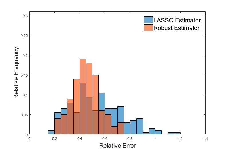
Figure 1: Lasso vs robust estimator without additive noise.

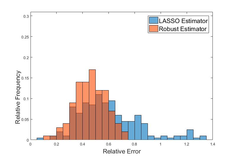
Figure 2: Lasso vs robust estimator under heavy-tailed noise with signal-to-noise ratio(SNR) equal to $10dB$.

In the second simulation study, the simulation framework similar to the second scenario above, the only difference being the increased sample size $m$. The results are plotted in Fig. 5-5 with sample sizes $m=128,~{}256$ and 512, respectively.

Figure 3: $m=128$

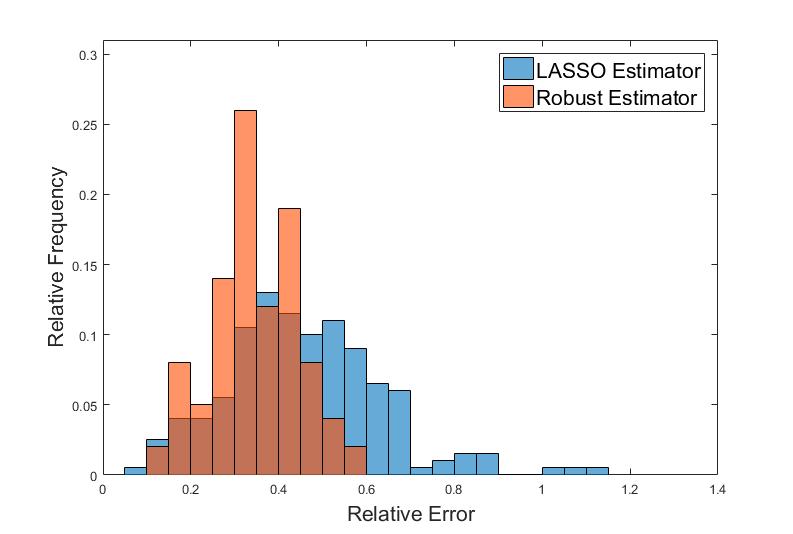
Figure 4: $m=256$

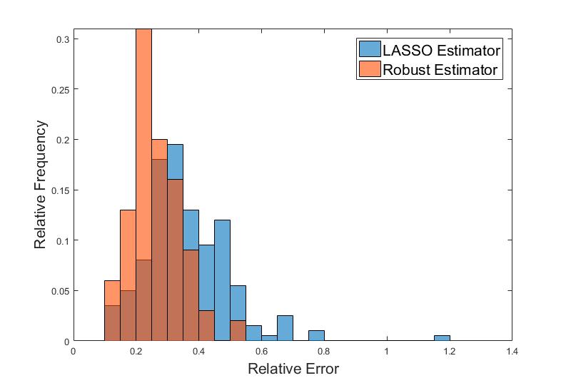
Figure 5: $m=512$

5 Proofs.

This section is devoted to the proofs of Theorems 3.1 and 3.2.

5.1 Preliminaries.

We recall several useful facts from probability theory that we rely on in the subsequent analysis.
The following well-known bound shows that the uniform distribution on a high-dimensional sphere enjoys strong concentration properties.

Lemma 5.1 (Lemma 2.2 of Ball (1997)).

Let $U$ have the uniform distribution on $\mathbb{S}^{d-1}$. Then for any $\Delta\in(0,1)$ and any fixed $\mathbf{v}\in\mathbb{S}^{d-1}$,

$$\mathbb{P}\left(\langle U,\mathbf{v}\rangle\geq\Delta\right)\leq e^{-d\Delta^{2}/2}.$$

Next, we state several useful results from the theory of empirical processes.

Definition 5.1 ($\psi_{q}$-norm).

For $q\geq 1$, the $\psi_{q}$-norm of a random variable $\xi\in\mathbb{R}$ is given by

$$\|\xi\|_{\psi_{q}}=\sup_{p\geq 1}p^{-\frac{1}{q}}(\mathbb{E}{\left(|X|^{p}\right)})^{\frac{1}{p}}.$$

Specifically, the cases $q=1$ and $q=2$ are known as the sub-exponential and sub-Gaussian norms respectively. We will say that $\xi$ is sub-exponential if $\|\xi\|_{\psi_{1}}<\infty$, and $X$ is sub-Gaussian if $\|\xi\|_{\psi_{2}}<\infty$.

Remark 5.1.

It is easy to check that $\psi_{q}$-norm is indeed a norm.

Remark 5.2.

A useful property, equivalent to the previous definition of a sub-Gaussian random variable $\xi$, is that there exists a positive constant $C$ such that

$$\mathbb{P}\left(|\xi|\geq u\right)\leq\exp(1-Cu^{2}).$$

For the proof, see Lemma 5.5 in Vershynin (2010).

Definition 5.2 (sub-Gaussian random vector).

A random vector $\mathbf{x}\in\mathbb{R}^{d}$ is called sub-Gaussian if there exists $C>0$ such that $\|\langle\mathbf{x},\mathbf{v}\rangle\|_{\psi_{2}}\leq C$ for any $\mathbf{v}\in\mathbb{S}^{d-1}$. The corresponding sub-Gaussian norm is then

$$\|\mathbf{x}\|_{\psi_{2}}:=\sup_{\mathbf{v}\in\mathbb{S}^{d-1}}\|\langle\mathbf{x},\mathbf{v}\rangle\|_{\psi_{2}}.$$

Next, we recall the notion of the generic chaining complexity. Let $(T,d)$ be a metric space. We say a collection $\{\mathcal{A}_{l}\}_{l=0}^{\infty}$ of subsets of $T$ is increasing when $\mathcal{A}_{l}\subseteq\mathcal{A}_{l+1}$ for all $l\geq 0$.

Definition 5.3 (Admissible sequence).

An increasing sequence of subsets $\{\mathcal{A}_{l}\}_{l=0}^{\infty}$ of $T$ is admissible if $|\mathcal{A}_{l}|\leq N_{l},~{}\forall l$, where $N_{0}=1$ and $N_{l}=2^{2^{l}},~{}\forall l\geq 1$.

For each $\mathcal{A}_{l}$, define the map $\pi_{l}:T\rightarrow\mathcal{A}_{l}$ as $\pi_{l}(t)=\textrm{arg}\min_{s\in\mathcal{A}_{l}}d(s,t),~{}\forall t\in T$. Note that, since each $\mathcal{A}_{l}$ is a finite set, the minimum is always achieved. When the minimum is achieved for multiple elements in $\mathcal{A}_{l}$, we break the ties arbitrarily. The generic chaining complexity $\gamma_{2}$ is defined as

$$\gamma_{2}(T,d):=\inf\sup_{t\in T}\sum_{l=0}^{\infty}2^{l/2}d(t,\pi_{l}(t)),$$ (21)

where the infimum is over all admissible sequences. The following theorem tells us that $\gamma_{2}$-functional controls the “size” of a Gaussian process.

Lemma 5.2 (Theorem 2.4.1 of Talagrand (2014)).

Let $\{G(t),\ t\in T\}$ be a centered Gaussian process indexed by the set $T$, and let

$$d(s,t)=\mathbb{E}{\left((G(s)-G(t))^{2}\right)}^{1/2},~{}\forall s,t\in T.$$

Then, there exists a universal constant $L$ such that

$$\frac{1}{L}\gamma_{2}(T,d)\leq\mathbb{E}{\left(\sup_{t\in T}G(t)\right)}\leq L\gamma_{2}(T,d).$$

Let $(T,d)$ be a semi-metric space, and let $X_{1}(t),\cdots,X_{m}(t)$ be independent stochastic processes indexed by $T$ such that $\mathbb{E}|X_{j}(t)|<\infty$ for all $t\in\mathbb{T}$ and $1\leq j\leq m$. We are interested in bounding the supremum of the empirical process

$$Z_{m}(t)=\frac{1}{m}\sum_{i=1}^{m}\left[X_{i}(t)-\mathbb{E}{\left(X_{i}(t)\right)}\right].$$ (22)

The following well-known symmetrization inequality reduces the problem to bounds on a (conditionally) Rademacher process $R_{m}(t)=\frac{1}{m}\sum_{i=1}^{m}\varepsilon_{i}X_{i}(t),~{}t\in T$, where $\varepsilon_{1},\ldots,\varepsilon_{m}$ are i.i.d. Rademacher random variables (meaning that they take values $\{-1,+1\}$ with probability $1/2$ each), independent of $X_{i}$’s.

Lemma 5.3 (Symmetrization inequalities).

$$\mathbb{E}\sup_{t\in T}|Z_{m}(t)|\leq 2\mathbb{E}\sup_{t\in T}|R_{m}(t)|,$$

and for any $u>0$, we have

$$\mathbb{P}\left(\sup_{t\in T}|Z_{m}(t)|\geq 2\mathbb{E}\sup_{t\in T}|Z_{m}(t)|+u\right)\leq 4\mathbb{P}\left(\sup_{t\in T}|R_{m}(t)|\geq u/2\right).$$

Proof.

See Lemmas 6.3 and 6.5 in (Ledoux and Talagrand, 1991) ∎

Finally, we recall Bernstein’s concentration inequality.

Lemma 5.4 (Bernstein’s inequality).

Let $X_{1},\cdots,X_{m}$ be a sequence of independent centered random variables. Assume that there exist positive constants $\sigma$ and $D$ such that for all integers $p\geq 2$

$$\frac{1}{m}\sum_{i=1}^{m}\mathbb{E}{\left(|X_{i}|^{p}\right)}\leq\frac{p!}{2}\sigma^{2}D^{p-2},$$

then

$$\mathbb{P}\left(\left|\frac{1}{m}\sum_{i=1}^{m}X_{i}\right|\geq\frac{\sigma}{\sqrt{m}}\sqrt{2u}+\frac{D}{m}u\right)\leq 2\exp(-u).$$

In particular, if $X_{1},\cdots,X_{m}$ are all sub-exponential random variables, then $\sigma$ and $D$ can be chosen as $\sigma=\frac{1}{m}\sum_{i=1}^{m}\|X_{i}\|_{\psi_{1}}$ and $D=\max\limits_{i=1\ldots m}\|X_{i}\|_{\psi_{1}}$.

5.2 Roadmap of the proof of Theorem 3.1.

We outline the main steps in the proof of Theorem 3.1, and postpone some technical details to sections 5.4 and 5.5.
As it will be shown below in Lemma 5.5, $\mathop{\mbox{argmin}}\limits_{\theta\in\Theta}L^{0}(\theta)=\eta\theta_{\ast}$ for $\eta=\mathbb{E}\left(\left\langle y\mathbf{x},\theta_{\ast}\right\rangle\right)$ and $L^{0}(\widehat{\theta}_{m})-L^{0}(\eta\theta_{\ast})=\|\widehat{\theta}_{m}-\eta\theta_{\ast}\|_{2}^{2}$, hence

$$\|\widehat{\theta}_{m}-\eta\theta_{\ast}\|_{2}^{2} =L^{\tau}(\widehat{\theta}_{m})-L^{\tau}(\eta\theta_{\ast})+\left(L^{0}(\widehat{\theta}_{m})-L^{\tau}(\widehat{\theta}_{m})-L^{0}(\eta\theta_{\ast})+L^{\tau}(\eta\theta_{\ast})\right)$$

$$=L^{\tau}(\widehat{\theta}_{m})-L^{\tau}(\eta\theta_{\ast})+(L_{m}^{\tau}(\widehat{\theta}_{m})-L_{m}^{\tau}(\eta\theta_{\ast}))$$

$$\quad-(L_{m}^{\tau}(\widehat{\theta}_{m})-L_{m}^{\tau}(\eta\theta_{\ast}))-2\mathbb{E}_{m}\left\langle y\mathbf{x}-\widetilde{q}\widetilde{U},\widehat{\theta}_{m}-\eta\theta_{\ast}\right\rangle,$$ (23)

where $\mathbb{E}_{m}(\cdot)$ stands for the conditional expectation given $(\mathbf{x}_{i},y_{i})_{i=1}^{m}$, and where we used the equality $L^{0}(\widehat{\theta}_{m})-L^{\tau}(\widehat{\theta}_{m})-L^{0}(\eta\theta_{\ast})+L^{\tau}(\eta\theta_{\ast})=-2\mathbb{E}_{m}\left(\left\langle y\mathbf{x}-\widetilde{q}\widetilde{U},\widehat{\theta}_{m}-\eta\theta_{\ast}\right\rangle\right)$ in the last step. Since $\widehat{\theta}_{m}$ minimizes $L_{m}^{\tau}$, $L_{m}^{\tau}(\widehat{\theta}_{m})-L_{m}^{\tau}(\eta\theta_{\ast})\leq 0$, and

$$\|\widehat{\theta}_{m}-\eta\theta_{\ast}\|_{2}^{2}\leq \,\frac{2}{m}\sum_{i=1}^{m}\left(\left\langle\widetilde{q}_{i}\widetilde{U}_{i},\widehat{\theta}_{m}-\eta\theta_{\ast}\right\rangle-\mathbb{E}_{m}\left(\left\langle\widetilde{q}\widetilde{U},\widehat{\theta}_{m}-\eta\theta_{\ast}\right\rangle\right)\right)$$

$$-2\mathbb{E}_{m}\left(\left\langle y\mathbf{x}-\widetilde{q}\widetilde{U},\widehat{\theta}_{m}-\eta\theta_{\ast}\right\rangle\right).$$

Note that $\widehat{\theta}_{m}-\eta\theta_{\ast}\in D(\Theta,\eta\theta_{\ast})$; dividing both sides of the inequality by $\|\widehat{\theta}_{m}-\eta\theta_{\ast}\|_{2}$, we obtain

$$\|\widehat{\theta}_{m}-\eta\theta_{\ast}\|_{2}\leq\sup_{\mathbf{v}\in D(\Theta,\eta\theta_{\ast})\cap\mathbb{S}^{d-1}}\left|\frac{2}{m}\sum_{i=1}^{m}\left\langle\widetilde{q}_{i}\widetilde{U}_{i},\mathbf{v}\right\rangle-\mathbb{E}\left\langle\widetilde{q}\widetilde{U},\mathbf{v}\right\rangle\right|+2\sup_{\mathbf{v}\in\mathbb{S}^{d-1}}\mathbb{E}\left\langle y\mathbf{x}-\widetilde{q}\widetilde{U},\mathbf{v}\right\rangle.$$ (24)

To get the desired bound, it remains to estimate two terms above. The bound for the first term is implied by Lemma 5.8: setting $T=D(\Theta,\eta\theta_{\ast})\cap\mathbb{S}^{d-1}$, and observing that the diameter $\Delta_{d}(T):=\sup_{t\in T}\|t\|_{2}=1$, we get that with probability $\geq 1-ce^{-\beta/2}$,

$$\sup_{\mathbf{v}\in D(\Theta,\eta\theta_{\ast})\cap\mathbb{S}^{d-1}}\left|\frac{2}{m}\sum_{i=1}^{m}\left\langle\widetilde{q}_{i}\widetilde{U}_{i},\mathbf{v}\right\rangle-\mathbb{E}\left\langle\widetilde{q}\widetilde{U},\mathbf{v}\right\rangle\right|\leq C\frac{(\omega(T)+1)\beta}{\sqrt{m}}.$$

To estimate the second term, we apply Lemma 5.7:

$$2\sup_{\mathbf{v}\in\mathbb{S}^{d-1}}\mathbb{E}\left\langle y\mathbf{x}-\widetilde{q}\widetilde{U},\mathbf{v}\right\rangle\ \leq\frac{\tilde{C}}{\sqrt{m}}.$$

Result of Theorem 3.1 now follows from the combination of these bounds. ∎

5.3 Roadmap of the proof of Theorem 3.2.

Once again, we will present the main steps while skipping the technical parts. Lemma 5.5 implies that $\mathop{\mbox{argmin}}\limits_{\theta\in\Theta}L^{0}(\theta)=\eta\theta_{\ast}$ for $\eta=\mathbb{E}\left\langle y\mathbf{x},\theta_{\ast}\right\rangle$ and

$$L^{0}(\widehat{\theta}_{m}^{\lambda})-L^{0}(\eta\theta_{\ast})=\|\widehat{\theta}_{m}^{\lambda}-\eta\theta_{\ast}\|_{2}^{2}.$$

Thus, arguing as in (23),

$$\|\widehat{\theta}_{m}^{\lambda}-\eta\theta_{\ast}\|_{2}^{2} =L^{\tau}(\widehat{\theta}_{m}^{\lambda})-L^{\tau}(\eta\theta_{\ast})+(L_{m}^{\tau}(\widehat{\theta}_{m}^{\lambda})-L_{m}^{\tau}(\eta\theta_{\ast}))$$

$$\quad-(L_{m}^{\tau}(\widehat{\theta}_{m}^{\lambda})-L_{m}^{\tau}(\eta\theta_{\ast}))-2\mathbb{E}_{m}\left\langle y\mathbf{x}-\widetilde{q}\widetilde{U},\widehat{\theta}_{m}^{\lambda}-\eta\theta_{\ast}\right\rangle.$$

Since $\widehat{\theta}^{\lambda}_{m}$ is a solution of problem (11), it follows that

$$L_{m}^{\tau}(\theta_{m}^{\lambda})+\lambda\left\|\theta_{m}^{\lambda}\right\|_{\mathcal{K}}\leq L_{m}^{\tau}\left(\eta\theta_{*}\right)+\lambda\left\|\eta\theta_{*}\right\|_{\mathcal{K}},$$

which further implies that

$$\|\widehat{\theta}_{m}^{\lambda}-\eta\theta_{*}\|_{2}^{2}\leq \frac{2}{m}\sum_{i=1}^{m}\left(\left\langle\widetilde{q}_{i}\widetilde{U}_{i},\widehat{\theta}_{m}^{\lambda}-\eta\theta_{\ast}\right\rangle-\mathbb{E}_{m}\left\langle\widetilde{q}\widetilde{U},\widehat{\theta}_{m}^{\lambda}-\eta\theta_{\ast}\right\rangle\right)-2\mathbb{E}_{m}\left\langle y\mathbf{x}-\widetilde{q}\widetilde{U},\widehat{\theta}_{m}^{\lambda}-\eta\theta_{\ast}\right\rangle$$

$$+\lambda\left(\|\eta\theta_{*}\|_{\mathcal{K}}-\|\widehat{\theta}_{m}^{\lambda}\|_{\mathcal{K}}\right)$$

$$= \left\langle\frac{2}{m}\sum_{i=1}^{m}\widetilde{q}_{i}\widetilde{U}_{i}-\mathbb{E}{\left(\widetilde{q}\widetilde{U}\right)},\widehat{\theta}_{m}^{\lambda}-\eta\theta_{\ast}\right\rangle-2\mathbb{E}_{m}\left\langle y\mathbf{x}-\widetilde{q}\widetilde{U},\widehat{\theta}_{m}^{\lambda}-\eta\theta_{\ast}\right\rangle$$

$$+\lambda\left(\|\eta\theta_{*}\|_{\mathcal{K}}-\|\widehat{\theta}_{m}^{\lambda}\|_{\mathcal{K}}\right).$$ (25)

Letting $\|\cdot\|_{\mathcal{K}}^{*}$ be the dual norm of $\|\cdot\|_{\mathcal{K}}$ (meaning that $\|\mathbf{x}\|_{\mathcal{K}}^{\ast}=\sup\left\{\left\langle\mathbf{x},\mathbf{z}\right\rangle,\ \|\mathbf{z}\|_{\mathcal{K}}\leq 1\right\}$), the first term in (25) can be estimated as

$$\left\langle\frac{1}{m}\sum_{i=1}^{m}\widetilde{q}_{i}\widetilde{U}_{i}-\mathbb{E}{\left(\widetilde{q}\widetilde{U}\right)},\widehat{\theta}_{m}^{\lambda}-\eta\theta_{\ast}\right\rangle\leq\left\|\frac{1}{m}\sum_{i=1}^{m}\widetilde{q}_{i}\widetilde{U}_{i}-\mathbb{E}{\left(\widetilde{q}\widetilde{U}\right)}\right\|_{\mathcal{K}}^{*}\cdot\|\widehat{\theta}_{m}^{\lambda}-\eta\theta_{*}\|_{\mathcal{K}}.$$ (26)

Since

$$\left\|\frac{1}{m}\sum_{i=1}^{m}\widetilde{q}_{i}\widetilde{U}_{i}-\mathbb{E}{\left(\widetilde{q}\widetilde{U}\right)}\right\|_{\mathcal{K}}^{*}=\sup_{\|t\|_{\mathcal{K}}\leq 1}\left\langle\frac{1}{m}\sum_{i=1}^{m}\widetilde{q}_{i}\widetilde{U}_{i}-\mathbb{E}{\left(\widetilde{q}\widetilde{U}\right)},t\right\rangle,$$

lemma 5.8 applies with $T=\mathcal{G}:=\{\mathbf{x}\in\mathbb{R}^{d}:~{}\|\mathbf{x}\|_{\mathcal{K}}\leq 1\}$. Together with an observation that $\Delta_{d}(T)\leq\sup_{t\in T}\|t\|_{\mathcal{K}}=1$ (due to the assumption $\|\mathbf{v}\|_{2}\leq\|\mathbf{v}\|_{\mathcal{K}},\ \forall\mathbf{v}\in\mathbb{R}^{d}$), this yiels

$$\mathbb{P}\left(\sup_{\|t\|_{\mathcal{K}}\leq 1}\left|\left\langle\frac{1}{m}\sum_{i=1}^{m}\widetilde{q}_{i}\widetilde{U}_{i}-\mathbb{E}{\left(\widetilde{q}\widetilde{U}\right)},t\right\rangle\right|\geq C^{\prime}\frac{\left(\omega(\mathcal{G})+1\right)\beta}{\sqrt{m}}\right)\leq c^{\prime}e^{-\beta/2},$$

for any $\beta\geq 8$ and some constants $C^{\prime},c>0$. For the second term in (25), we use Lemma 5.7 to obtain

$$2\mathbb{E}_{m}\left\langle y\mathbf{x}-\widetilde{q}\widetilde{U},\widehat{\theta}_{m}^{\lambda}-\eta\theta_{\ast}\right\rangle\leq\frac{C^{\prime\prime}}{\sqrt{m}}\|\widehat{\theta}_{m}^{\lambda}-\eta\theta_{*}\|_{2}\leq\frac{C^{\prime\prime}}{\sqrt{m}}\|\widehat{\theta}_{m}^{\lambda}-\eta\theta_{*}\|_{\mathcal{K}},$$

for some constant $C^{\prime\prime}>0$, where we have again applied the inequality $\|\mathbf{v}\|_{2}\leq\|\mathbf{v}\|_{\mathcal{K}}$. Combining the above two estimates gives that with probability at least $1-ce^{-\beta/2}$,

$$\|\widehat{\theta}_{m}^{\lambda}-\eta\theta_{*}\|_{2}^{2}\leq C\frac{\left(\omega(\mathcal{G})+1\right)\beta}{\sqrt{m}}\|\widehat{\theta}_{m}^{\lambda}-\eta\theta_{*}\|_{\mathcal{K}}+\lambda\left(\|\eta\theta_{*}\|_{\mathcal{K}}-\|\widehat{\theta}_{m}^{\lambda}\|_{\mathcal{K}}\right),$$ (27)

for some constant $C>0$ and any $\beta\geq 8$. Since $\lambda\geq 2C\left(\omega(\mathcal{G})+1\right)\beta/\sqrt{m}$ by assumption, and the right hand side of (27) is nonnegative, it follows that

$$\frac{1}{2}\|\widehat{\theta}_{m}^{\lambda}-\eta\theta_{*}\|_{\mathcal{K}}+\|\eta\theta_{*}\|_{\mathcal{K}}-\|\widehat{\theta}_{m}^{\lambda}\|_{\mathcal{K}}\geq 0.$$

This inequality implies that $\widehat{\theta}_{m}^{\lambda}-\eta\theta_{*}\in\mathbb{S}_{2}(\eta\theta_{*})$. Finally, from (27) and the triangle inequality,

$$\|\widehat{\theta}_{m}^{\lambda}-\eta\theta_{*}\|_{2}^{2}\leq\frac{3}{2}\lambda\|\widehat{\theta}_{m}^{\lambda}-\eta\theta_{*}\|_{\mathcal{K}}.$$

Dividing both sides by $\|\widehat{\theta}_{m}^{\lambda}-\eta\theta_{*}\|_{2}$ gives

$$\|\widehat{\theta}_{m}^{\lambda}-\eta\theta_{*}\|_{2}\leq\frac{3}{2}\lambda\frac{\|\widehat{\theta}_{m}^{\lambda}-\eta\theta_{*}\|_{\mathcal{K}}}{\|\widehat{\theta}_{m}^{\lambda}-\eta\theta_{*}\|_{2}}\leq\frac{3}{2}\lambda\cdot\Psi\left(\mathbb{S}_{2}(\eta\theta_{*})\right).$$

This finishes the proof of Theorem 3.2.

5.4 Bias of the truncated mean.

The following lemma is motivated by and is similar to Theorem 2.1 in (Li and Duan, 1989).

Lemma 5.5.

Let $\eta=\mathbb{E}\langle y\mathbf{x},\theta_{\ast}\rangle$. Then

$$\eta\theta_{\ast}=\mathop{\mbox{argmin}}_{\theta\in\Theta}L^{0}(\theta),$$

and for any $\theta\in\Theta$,

$$L^{0}(\theta)-L^{0}(\eta\theta_{\ast})=\|\theta-\eta\theta_{\ast}\|_{2}^{2}.$$

Proof.

Since $y=f(\left\langle\mathbf{x},\theta_{*}\right\rangle,\delta)$, we have that for any $\theta\in\mathbb{R}^{d}$

$$\mathbb{E}\left\langle y\mathbf{x},\theta\right\rangle= \mathbb{E}\langle\mathbf{x},\theta\rangle f(\langle\mathbf{x},\theta_{*}\rangle,\delta)$$

$$= \mathbb{E}\mathbb{E}{\left(\langle\mathbf{x},\theta\rangle f(\langle\mathbf{x},\theta_{*}\rangle,\delta)~{}|~{}\langle\mathbf{x},\theta_{*}\rangle,\delta\right)}$$

$$= \mathbb{E}\mathbb{E}\left(\langle\mathbf{x},\theta\rangle~{}|~{}\langle\mathbf{x},\theta_{*}\rangle\right)\cdot f(\langle\mathbf{x},\theta_{*}\rangle,\delta)$$

$$= \mathbb{E}\Big{(}\langle\theta_{*},\theta\rangle\langle\mathbf{x},\theta_{*}\rangle f(\langle\mathbf{x},\theta_{*}\rangle,\delta)\Big{)}$$

$$= \eta\langle\theta_{*},\theta\rangle,$$

where the third equality follows from the fact that the noise $\delta$ is independent of the measurement vector $\mathbf{x}$, the second to last equality from the properties of elliptically symmetric distributions (Corollary 2.1), and the last equality from the definition of $\eta$. Thus,

$$L^{0}(\theta)= \|\theta\|_{2}^{2}-2\mathbb{E}{\left(\left\langle y\mathbf{x},\theta\right\rangle\right)}=\|\theta\|_{2}^{2}-2\eta\langle\theta_{*},\theta\rangle=\|\theta-\eta\theta_{*}\|_{2}^{2}-\|\eta\theta_{*}\|_{2}^{2},$$

which is minimized at $\theta=\eta\theta^{*}$. Furthermore, $L^{0}(\eta\theta^{*})=-\|\eta\theta_{*}\|_{2}^{2}$, hence

$$L^{0}(\theta)-L^{0}(\eta\theta_{\ast})=\|\theta-\eta\theta_{\ast}\|_{2}^{2},$$

finishing the proof. ∎

Next, we estimate the “bias term” $\sup_{\mathbf{v}\in\mathbb{S}^{d-1}}\mathbb{E}\left\langle y\mathbf{x}-\widetilde{q}\widetilde{U},\mathbf{v}\right\rangle$ in inequality (24). In order to do so, we need the following preliminary result.

Lemma 5.6.

If $\mathbf{x}\sim\mathcal{E}(0,~{}\mathbf{I}_{d\times d},~{}F_{\mu})$, then the unit random vector $\mathbf{x}/\|\mathbf{x}\|_{2}$ is uniformly distributed over the unit sphere $\mathbb{S}^{d-1}$. Furthermore, $\widetilde{U}=\sqrt{d}\mathbf{x}/\|\mathbf{x}\|_{2}$ is a sub-Gaussian random vector with sub-Gaussian norm $\|\widetilde{U}\|_{\psi_{2}}$ independent of the dimension $d$.

Proof.

First, we use decomposition (3) for elliptical distribution together with our assumption that $\mathbf{\Sigma}$ is the identity matrix, to write $\mathbf{x}\stackrel{{\scriptstyle d}}{{=}}\mu U$, which implies that

$$\mathbf{x}/\|\mathbf{x}\|_{2}\stackrel{{\scriptstyle d}}{{=}}\textrm{sign}(\mu)U/\|U\|_{2}=\textrm{sign}(\mu)U\stackrel{{\scriptstyle d}}{{=}}U,$$

with the final distributional equality holding as $\mathbb{S}^{d-1}$, and hence its uniform distribution, is invariant with respect to reflections across any hyperplane through the origin.

To prove the second claim, it is enough to show that $\left\|\left\langle\widetilde{U},\mathbf{v}\right\rangle\right\|_{\psi_{2}}\leq C,~{}\forall\mathbf{v}\in\mathbb{S}^{d-1}$ with constant $C$ independent of $d$. By the first claim and Lemma 5.1, we have

$$\mathbb{P}\left(\langle\mathbf{x},\mathbf{v}\rangle/\|\mathbf{x}\|_{2}\geq\Delta\right)\leq e^{-d\Delta^{2}/2},~{}\forall\mathbf{v}\in\mathbb{S}^{d-1}.$$

Choosing $\Delta=u/\sqrt{d}$ gives

$$\mathbb{P}\left(\left\langle\widetilde{U},\mathbf{v}\right\rangle\geq u\right)\leq e^{-u^{2}/2},~{}\forall\mathbf{v}\in\mathbb{S}^{d-1},~{}\forall u>0.$$

By an equivalent definition of sub-Gaussian random variables (Lemma 5.5 of Vershynin (2010)), this inequality implies that $\left\|\left\langle\widetilde{U},\mathbf{v}\right\rangle\right\|_{\psi_{2}}\leq C$, hence finishing the proof. ∎

With the previous lemma in hand, we now establish the following result.

Lemma 5.7.

Under the assumptions of Theorem 3.1, there exists a constant $C=C(\kappa,\phi)>0$ such that

$$\left|\mathbb{E}\left\langle y\mathbf{x}-\widetilde{q}\widetilde{U},\mathbf{v}\right\rangle\right|\leq C/\sqrt{m},$$

for all $\mathbf{v}\in\mathbb{S}^{d-1}$.

Proof.

By (6), we have that $y\mathbf{x}=q\widetilde{U}$, thus the claim is equivalent to

$$\left|\mathbb{E}{\left(\left\langle\widetilde{U},\mathbf{v}\right\rangle(\widetilde{q}-q)\right)}\right|\leq C/\sqrt{m}.$$

Since $\widetilde{q}=\textrm{sign}(q)(|q|\wedge\tau)$, we have $|\widetilde{q}-q|=(|q|-\tau){\bf 1}(|q|\geq\tau)\leq|q|{\bf 1}(|q|\geq\tau)$, and it follows that

$$\left|\mathbb{E}\left\langle\widetilde{U},\mathbf{v}\right\rangle(\widetilde{q}-q)\right|\leq \mathbb{E}\left|\left\langle\widetilde{U},\mathbf{v}\right\rangle(\widetilde{q}-q)\right|$$

$$\leq \mathbb{E}\left(\left|\left\langle\widetilde{U},\mathbf{v}\right\rangle q\right|\cdot\mathbf{1}_{\{|q|\geq\tau\}}\right)$$

$$\leq \mathbb{E}{\left(\left|\left\langle\widetilde{U},\mathbf{v}\right\rangle q\right|^{2}\right)}^{1/2}\mathbb{P}\left(|q|\geq\tau\right)^{1/2}$$

$$\leq \mathbb{E}{\left(\left|\left\langle\widetilde{U},\mathbf{v}\right\rangle\right|^{\frac{2(1+\kappa)}{\kappa}}\right)}^{\frac{\kappa}{2(1+\kappa)}}\mathbb{E}{\left(|q|^{2(1+\kappa)}\right)}^{\frac{1}{2(1+\kappa)}}\mathbb{P}\left(|q|\geq\tau\right)^{1/2},$$

where the second to last inequality uses Cauchy-Schwarz, and the last inequality follows from Hölder’s inequality.

For the first term, by Lemma 5.6, $\widetilde{U}$ is sub-Gaussian with $\|\widetilde{U}\|_{\psi_{2}}$ independent of $d$. Thus, by the definition of the $\|\cdot\|_{\psi_{2}}$ norm and the fact that ${\bf v}\in\mathbb{S}^{d-1}$,

$$\mathbb{E}{\left(\left|\left\langle\widetilde{U},\mathbf{v}\right\rangle\right|^{\frac{2(1+\kappa)}{\kappa}}\right)}^{\frac{\kappa}{2(1+\kappa)}}\leq\sqrt{\frac{2(1+\kappa)}{\kappa}}\|\widetilde{U}\|_{\psi_{2}}.$$

Recall that $\phi=\mathbb{E}|q|^{2(1+\kappa)}$. Then, the second term is bounded by $\phi^{\frac{1}{2(1+\kappa)}}$. For the final term, since $\tau=m^{\frac{1}{2(1+\kappa)}}$, Markov’s inequality implies that

$$\left(\mathbb{P}\left(|q|>\tau\right)\right)^{1/2}\leq\left(\frac{\mathbb{E}|q|^{2(1+\kappa)}}{\tau^{2(1+\kappa)}}\right)^{1/2}\leq\frac{\phi^{1/2}}{\sqrt{m}}.$$

Combining these inequalities yields

$$\left|\mathbb{E}\left\langle y\mathbf{x}-\widetilde{q}\widetilde{U},\mathbf{v}\right\rangle\right|\leq\frac{\sqrt{\frac{2(1+\kappa)}{\kappa}}\|\widetilde{U}\|_{\psi_{2}}\phi^{\frac{2+\kappa}{2(1+\kappa)}}}{\sqrt{m}}:=C(\kappa,\phi)/\sqrt{m},$$

completing the proof. ∎

5.5 Concentration via generic chaining.

In the following sections, we will use $c,C,C^{\prime},C^{\prime\prime}$ to denote constants that are either absolute, or depend on underlying parameters $\kappa$ and $\phi$ (in the latter case, we specify such dependence). To make notation less cumbersome, constants denoted by the same letter ($c,C,C^{\prime}$, etc.) might be different in various parts of the proof.

The goal of this subsection is to prove the following inequality:

Lemma 5.8.

Suppose $\widetilde{U}_{i}$ and $\widetilde{q}_{i}$ are as defined according to (6) and (7) respectively. Then, for any bounded subset $T\subset\mathbb{R}^{d}$,

$$\mathbb{P}\left(\sup_{t\in T}\left|\frac{1}{m}\sum_{i=1}^{m}\left\langle\widetilde{U}_{i},t\right\rangle\widetilde{q}_{i}-\mathbb{E}{\left(\left\langle\widetilde{U},t\right\rangle\widetilde{q}\right)}\right|\geq C\frac{(\omega(T)+\Delta_{d}(T))\beta}{\sqrt{m}}\right)\leq ce^{-\beta/2},$$

for any $\beta\geq 8$, a positive constant $C=C(\kappa,\phi)$ and an absolute constant $c>0$. Here

$$\Delta_{d}(T):=\sup_{t\in T}\|t\|_{2}.$$ (28)

The main technique we apply is the generic chaining method developed by M. Talagrand (Talagrand, 2014) for bounding the supremum of stochastic processes. Recently, Mendelson, Pajor and Tomczak-Jaegermann (2007) and Dirksen (2013) advanced the technique to obtain a sharp bound for supremum of processes index by squares of functions. More recently, Mendelson (2014) proved a concentration result for the supremum of multiplier processes under weak moment assumptions. In the current work, we show that exponential-type concentration inequalities for multiplier processes, such as the one in Lemma 5.8, are achievable by applying truncation under a bounded $2(1+\kappa)$-moment assumption.

Define

$$\overline{Z}(t)= \frac{1}{m}\sum_{i=1}^{m}\left\langle\widetilde{U}_{i},t\right\rangle\widetilde{q}_{i}-\mathbb{E}{\left(\left\langle\widetilde{U},t\right\rangle\widetilde{q}\right)},$$

$$Z(t)= \frac{1}{m}\sum_{i=1}^{m}\varepsilon_{i}\widetilde{q}_{i}\left\langle\widetilde{U}_{i},t\right\rangle,~{}\forall t\in T,$$

where $T$ is a bounded set in $\mathbb{R}^{d}$ and $\{\varepsilon_{i}\}_{i=1}^{m}$ is a sequence i.i.d. Rademacher random variables taking values $\pm 1$ with probability $1/2$ each, and independent of $\{\widetilde{U}_{i},\widetilde{q}_{i},\ i=1,\ldots,m\}$. Result of Lemma 5.8 easily follows from the following concentration inequality:

Lemma 5.9.

For any $\beta\geq 8$,

$$\mathbb{P}\left[\sup_{t\in T}\left|Z(t)\right|\geq C\frac{(\omega(T)+\Delta_{d}(T))\beta}{\sqrt{m}}\right]\leq ce^{-\beta/2},$$ (29)

where $C=C(\kappa,\phi)$ is another constant possibly different from that of Lemma 5.8, and $c>0$ is an absolute constant.

To deduce the inequality of Lemma 5.8, we first apply the symmetrization inequality (Lemma 5.3), followed by Lemma A.1 with $\beta_{0}=8$. It implies that

$$\mathbb{E}{\left(\sup_{t\in T}\left|\overline{Z}(t)\right|\right)}\leq 2\mathbb{E}{\left(\sup_{t\in T}\left|Z(t)\right|\right)}\leq 2C\left(8+2ce^{-4}\right)\frac{\omega(T)+\Delta_{d}(T)}{\sqrt{m}}.$$

Application of the second bound of the symmetrization lemma with $u=2C(\omega(T)+\Delta_{d}(T))\beta/\sqrt{m}$ and (29) completes the proof of Lemma 5.8.

It remains to justify (29). We start by picking an arbitrary point $t_{0}\in T$ such that there exists an admissible sequence $\{t_{0}\}=\mathcal{A}_{0}\subseteq\mathcal{A}_{1}\subseteq\mathcal{A}_{2}\subseteq\cdots$ satisfying

$$\sup_{t\in T}\sum_{l=0}^{\infty}2^{l/2}\|\pi_{l}(t)-t\|_{2}\leq 2\gamma_{2}(T),$$ (30)

where we recall that $\pi_{l}$ is the closest point map from $T$ to $\mathcal{A}_{l}$ and the factor 2 is introduced so as to deal with the case where the infimum in the definition (21) of $\gamma_{2}(T)$ is not achieved. Then, write $Z(t)-Z(t_{0})$ as the telescoping sum:

$$Z(t)-Z(t_{0})=\sum_{l=1}^{\infty}Z(\pi_{l}(t))-Z(\pi_{l-1}(t))=\sum_{l=1}^{\infty}\frac{1}{m}\sum_{i=1}^{m}\varepsilon_{i}\widetilde{q}_{i}\left\langle\widetilde{U}_{i},\pi_{l}(t)-\pi_{l-1}(t)\right\rangle.$$

We claim that the telescoping sum converges with probability 1 for any $t\in T$. Indeed, note that for each fixed set of realizations of $\{\mathbf{x}_{i}\}_{i=1}^{m}$ and $\{\varepsilon_{i}\}_{i=1}^{m}$, each summand is bounded as

$$|\varepsilon_{i}\widetilde{q}_{i}\langle\widetilde{U}_{i},\pi_{l}(t)-\pi_{l-1}(t)\rangle|\leq|\widetilde{q}_{i}|\|\widetilde{U}_{i}\|_{2}\|\pi_{l}(t)-\pi_{l-1}(t)\|_{2}\leq|\widetilde{q}_{i}|\|\widetilde{U}_{i}\|_{2}(\|\pi_{l}(t)-t\|_{2}+\|\pi_{l-1}(t)-t\|_{2}).$$

Furthermore, since $T$ is a compact subset of $\mathbb{R}^{d}$, its Gaussian mean width is finite. Thus, by lemma 5.2, $\gamma_{2}(T)\leq L\omega(T)<\infty$. This inequality further implies that the sum on the left hand side of (30) converges with probability 1.

Next, with $\beta\geq 8$ being fixed, we split the index set $\{l\geq 1\}$ into the following three subsets:

$$I_{1} =\{l\geq 1:2^{l}\beta<\log em\};$$

$$I_{2} =\{l\geq 1:\log em\leq 2^{l}\beta<m\};$$

$$I_{3} =\{l\geq 1:2^{l}\beta\geq m\}.$$

By the assumptions in Theorem 3.1 and the bound $\beta\geq 8$, we have that $m\geq(\omega(T)+1)^{2}\beta^{2}\geq 64$, implying that $\log em=1+\log m<m$, and hence these three index sets are well defined. Depending on $\beta$, some of them might be empty, but this only simplifies our argument by making the partial sum over such an index set equal 0.

The following argument yields a bound for $Z(\pi_{l}(t))-Z(\pi_{l-1}(t))$, assuming all three index sets are nonempty. Specifically, we show that

$$\mathbb{P}\left(\sup_{t\in T}\left|\sum_{l\in I_{j}}\left(Z(\pi_{l}(t))-Z(\pi_{l-1}(t))\right)\right|\geq C\frac{\gamma_{2}(T)\beta}{\sqrt{m}}\right)\leq ce^{-\beta/2},$$ (31)

for $C=C(\kappa,\phi)$ and $j=1,2,3$, respectively.

5.5.1 The case $l\in I_{1}$.

Proof of inequality (31) for the index set $I_{1}$.

Recall that $\tau=m^{\frac{1}{2(1+\kappa)}}$.
For each $t\in T$ we apply Bernstein’s inequality (Lemma 5.4) to estimate each summand

$$Z(\pi_{l}(t))-Z(\pi_{l-1}(t))=\frac{1}{m}\sum_{i=1}^{m}\varepsilon_{i}\widetilde{q}_{i}\left\langle\widetilde{U}_{i},\pi_{l}(t)-\pi_{l-1}(t)\right\rangle.$$

For any integer $p\geq 2$, we have the following chains of inequalities:

$$\mathbb{E}{\left(\left|\varepsilon\widetilde{q}\left\langle\widetilde{U},\pi_{l}(t)-\pi_{l-1}(t)\right\rangle\right|^{p}\right)}$$

$$\leq \mathbb{E}{\left(\left|\varepsilon\left\langle\widetilde{U},\pi_{l}(t)-\pi_{l-1}(t)\right\rangle\right|^{p}q^{2}\cdot|\widetilde{q}|^{p-2}\right)}$$

$$\leq \mathbb{E}{\left(\left|\left\langle\widetilde{U},\pi_{l}(t)-\pi_{l-1}(t)\right\rangle\right|^{p}q^{2}\right)}\cdot\tau^{p-2}$$

$$\leq \tau^{p-2}\mathbb{E}{\left(\left|\left\langle\widetilde{U},\pi_{l}(t)-\pi_{l-1}(t)\right\rangle\right|^{\frac{1+\kappa}{\kappa}p}\right)}^{\frac{\kappa}{1+\kappa}}\mathbb{E}{\left(q^{2(1+\kappa)}\right)}^{\frac{1}{1+\kappa}}$$

$$\leq \tau^{p-2}\|\widetilde{U}\|_{\psi_{2}}^{p}\left(\frac{(1+\kappa)p}{\kappa}\right)^{p/2}\phi^{\frac{1}{1+\kappa}}\|\pi_{l}(t)-\pi_{l-1}(t)\|_{2}^{p},$$

where the second inequality follows from the truncation bound, the third from Hölder’s inequality, and the last from the assumption that $\mathbb{E}{\left(q^{2(1+\kappa)}\right)}\leq\phi$ and the following bound: by Lemma 5.6, $\widetilde{U}_{i}$ is sub-Gaussian, hence for any $p\geq 2$

$$\left(\mathbb{E}\left\langle\widetilde{U}_{i},\mathbf{v}\right\rangle^{\frac{1+\kappa}{\kappa}p}\right)^{\frac{\kappa}{(1+\kappa)p}}\leq\left(\frac{(1+\kappa)p}{\kappa}\right)^{1/2}\|\widetilde{U}_{i}\|_{\psi_{2}}\|\mathbf{v}\|_{2},~{}\forall\mathbf{v}\in\mathbb{R}^{d}.$$

We also note that $\|\widetilde{U}_{i}\|_{\psi_{2}}$ does not depend on $d$ by Lemma 5.6. Next, by Stirling’s approximation, $p!\geq\sqrt{2\pi}\sqrt{p}(p/e)^{p}$, thus there exist constants $C^{\prime}=C^{\prime}(\kappa,\phi)$ and $C^{\prime\prime}=C^{\prime\prime}(\kappa)$ such that

$$\mathbb{E}\left|\varepsilon\widetilde{q}\left\langle\widetilde{U},\pi_{l}(t)-\pi_{l-1}(t)\right\rangle\right|^{p}\leq\frac{p!}{2}C^{\prime}\|\pi_{l}(t)-\pi_{l-1}(t)\|_{2}^{2}(C^{\prime\prime}\tau\|\pi_{l}(t)-\pi_{l-1}(t)\|_{2})^{p-2}.$$

Bernstein’s inequality (Lemma 5.4), with $\sigma=C^{\prime}\|\pi_{l}(t)-\pi_{l-1}(t)\|_{2}$, $D=C^{\prime\prime}\tau\|\pi_{l}(t)-\pi_{l-1}(t)\|_{2}$ with $\tau=m^{1/2(1+\kappa)}$ now implies

$$\mathbb{P}\left(\left|\frac{1}{m}\sum_{i=1}^{m}\varepsilon_{i}\widetilde{q}_{i}\left\langle\widetilde{U}_{i},\pi_{l}(t)-\pi_{l-1}(t)\right\rangle\right|\geq\left(\frac{C^{\prime}\sqrt{2u}}{\sqrt{m}}+\frac{C^{\prime\prime}u}{m^{1-\frac{1}{2(1+\kappa)}}}\right)\|\pi_{l}(t)-\pi_{l-1}(t)\|_{2}\right)\leq 2e^{-u},$$

for any $u>0$. Taking $u=2^{l}\beta$, noting that as $\beta\geq 8$ by assumption, we have $m\geq(\omega(T)+1)^{2}\beta^{2}\geq 64$, and since $l\in I_{1}$, $2^{l}\leq 2^{l}\beta<\log em$. In turn, this implies

$$\frac{2^{l}}{m^{1-\frac{1}{2(1+\kappa)}}}=\frac{2^{l/2}}{m^{1/2}}\cdot\frac{2^{l/2}}{m^{\kappa/2(1+\kappa)}}\leq\frac{2^{l/2}}{m^{1/2}}\cdot\sqrt{\frac{\log em}{m^{\kappa/(1+\kappa)}}}\leq\sqrt{\frac{1+\kappa}{\kappa}}\frac{2^{l/2}}{m^{1/2}},$$

where the last inequality follows from the fact that $\log em$ is dominated by $\frac{1+\kappa}{\kappa}m^{\kappa/(1+\kappa)}$ for all $m\geq 1$. This inequality implies that there exists a positive constant $C=C(\kappa,\phi)$ such that for any $\beta\geq 8$

$$\mathbb{P}\left(\Omega_{l,t}\right)\leq 2\exp(-2^{l}\beta),$$ (32)

where for all $l\geq 1$ and $t\in T$ we let

$$\Omega_{l,t}=\left\{\omega:\left|\frac{1}{m}\sum_{i=1}^{m}\varepsilon_{i}\widetilde{q}_{i}\left\langle\widetilde{U}_{i},\pi_{l}(t)-\pi_{l-1}(t)\right\rangle\right|\geq C\frac{2^{l/2}\beta}{\sqrt{m}}\|\pi_{l}(t)-\pi_{l-1}(t)\|_{2}\right\}.$$

Notice that for each $l\geq 1$ the number of pairs $(\pi_{l}(t),\pi_{l-1}(t))$ appearing in the sum in (31) can be bounded by $|\mathcal{A}_{l}|\cdot|\mathcal{A}_{l-1}|\leq 2^{2^{l+1}}$. Thus, by a union bound and (32),

$$\mathbb{P}\left(\bigcup_{t\in T}\Omega_{l,t}\right)\leq\ 2\cdot 2^{2^{l+1}}\exp(-2^{l}\beta),$$

and hence,

$$\mathbb{P}\left(\bigcup_{l\in I_{1},t\in T}\Omega_{l,t}\right)\leq \sum_{l\in I_{1}}2\cdot 2^{2^{l+1}}\exp(-2^{l}\beta)$$

$$\leq \sum_{l\in I_{1}}2\cdot 2^{2^{l+1}}\exp\left(-2^{l-1}\beta-\beta/2\right)\leq ce^{-\beta/2},$$

for some absolute constant $c>0$, where in the last inequality we use the fact $\beta\geq 8$ to get a geometrically decreasing sequence. Thus, on the complement of the event $\cup_{l\in I_{1},t\in T}\Omega_{l,t}$, we have that with probability at least $1-ce^{-\beta/2}$,

$$\sup_{t\in T}\left|\sum_{l\in I_{1}}\left(Z(\pi_{l}(t))-Z(\pi_{l-1}(t))\right)\right|\leq \sup_{t\in T}\sum_{l\in I_{1}}\left|Z(\pi_{l}(t))-Z(\pi_{l-1}(t))\right|$$

$$\leq \sup_{t\in T}C\sum_{l\in I_{1}}\frac{2^{l/2}\beta}{\sqrt{m}}\|\pi_{l}(t)-\pi_{l-1}(t)\|_{2}$$

$$\leq \sup_{t\in T}C\sum_{l=1}^{\infty}\frac{2^{l/2}\beta}{\sqrt{m}}\|\pi_{l}(t)-\pi_{l-1}(t)\|_{2}$$

$$\leq 4C\frac{\gamma_{2}(T)\beta}{\sqrt{m}},$$

for $C=C(\kappa,\phi)$, where the last inequality follows from triangle inequality $\|\pi_{l}(t)-\pi_{l-1}(t)\|_{2}\leq\|\pi_{l-1}(t)-t\|_{2}+\|\pi_{l}(t)-t\|_{2}$ and (30). This proves the inequality (31) for $l\in I_{1}$. ∎

5.5.2 The case $l\in I_{2}$.

This is the most technically involved case of the three. For any fixed $t\in T$ and $l\in I_{2}$, we let $X_{i}=\widetilde{q}_{i}\left\langle\widetilde{U}_{i},\pi_{l}(t)-\pi_{l-1}(t)\right\rangle$ and $w_{i}=\langle\widetilde{U}_{i},\pi_{l}(t)-\pi_{l-1}(t)\rangle$. Then $X_{i}=\widetilde{q}_{i}w_{i}$ and

$$Z(\pi_{l}(t))-Z(\pi_{l-1}(t))=\frac{1}{m}\sum_{i=1}^{m}\varepsilon_{i}X_{i}=\frac{1}{m}\sum_{i=1}^{m}\varepsilon_{i}w_{i}\widetilde{q}_{i}.$$ (33)

For every fixed $k\in\{1,2,\cdots,m-1\}$ and fixed $u>0$, we bound the summation using the following inequality

$$\mathbb{P}\left(\left|\sum_{i=1}^{m}\varepsilon_{i}X_{i}\right|\geq\sum_{i=1}^{k}X^{*}_{i}+u\left(\sum_{i=k+1}^{m}(X_{i}^{*})^{2}\right)^{1/2}\right)\leq 2\exp(-u^{2}/2),$$

where $\{X_{i}^{*}\}_{i=1}^{m}$ is the non-increasing rearrangement of $\{|X_{i}|\}_{i=1}^{m}$ and $\{\varepsilon_{i}\}_{i=1}^{m}$ is a sequence of i.i.d. Rademancher random variables independent of $\{X_{i}\}_{i=1}^{m}$.

Remark 5.3.

This bound was first stated and proved in Montgomery-Smith (1990) with a sequence of fixed constants $\{X_{i}\}_{i=1}^{m}$. The current form can be obtained using independence property and conditioning on $\{X_{i}\}_{i=1}^{m}$. Furthermore, Montgomery-Smith (1990) tells us that the optimal choice of $k$ is at $\mathcal{O}(u^{2})$ Applications of this inequality to generic chaining-type arguments were previously introduced by Mendelson (2014).

Letting $J$ be the set of indices of the variables corresponding to the $k$ largest coordinates of $\{|w_{i}|\}_{i=1}^{m}$ and of $\{|\widetilde{q}_{i}|\}_{i=1}^{m}$, we have $|J|\leq 2k$ and with probability at least $1-2\exp(-u^{2}/2)$

$$\left|\sum_{i=1}^{m}\varepsilon_{i}X_{i}\right| \leq\sum_{i\in J}X^{*}_{i}+u\left(\sum_{i\in J^{c}}(X_{i}^{*})^{2}\right)^{1/2}$$

$$\leq 2\sum_{i=1}^{k}w_{i}^{*}\widetilde{q}_{i}^{*}+u\left(\sum_{i\in J^{c}}(w_{i}^{*}\widetilde{q}_{i}^{*})^{2}\right)^{1/2}$$

$$\leq 2\left(\sum_{i=1}^{k}(w_{i}^{*})^{2}\right)^{1/2}\left(\sum_{i=1}^{k}(\widetilde{q}_{i}^{*})^{2}\right)^{1/2}+u\left(\sum_{i=k+1}^{m}(w_{i}^{*})^{\frac{2(1+\kappa)}{\kappa}}\right)^{\frac{\kappa}{2(1+\kappa)}}\left(\sum_{i=k+1}^{m}(\widetilde{q}_{i}^{*})^{2(1+\kappa)}\right)^{\frac{1}{2(1+\kappa)}}$$

$$\leq 2\left(\sum_{i=1}^{k}(w_{i}^{*})^{2}\right)^{1/2}\left(\sum_{i=1}^{m}\widetilde{q}_{i}^{2}\right)^{1/2}+u\left(\sum_{i=k+1}^{m}(w_{i}^{*})^{\frac{2(1+\kappa)}{\kappa}}\right)^{\frac{\kappa}{2(1+\kappa)}}\left(\sum_{i=1}^{m}\widetilde{q}_{i}^{2(1+\kappa)}\right)^{\frac{1}{2(1+\kappa)}}$$ (34)

where the second to last inequality is a consequence of Hölder’s inequality. We take $u=2^{(l+1)/2}\sqrt{\beta}$. The key is to pick an appropriate cut point $k$ for each $l\in I_{2}$. Here, we choose $k=\lfloor 2^{l}\beta/\log(em/2^{l}\beta)\rfloor$, which makes $k=\mathcal{O}(2^{l}\beta)$ and also guarantees that $k\in\{1,2,\cdots,m-1\}$; see Lemma A.4. Under this choice, we have the following lemma:

Lemma 5.10.

Let $k=\lfloor 2^{l}\beta/\log(em/2^{l}\beta)\rfloor$, $w_{i}=\left\langle\widetilde{U}_{i},\pi_{l}(t)-\pi_{l-1}(t)\right\rangle$ and $\{w_{i}^{*}\}_{i=1}^{m}$ be the nonincreasing rearrangement of $\{|w_{i}|\}_{i=1}^{m}$. Then there exists an absolute constant $C>1$ such that for all $\beta\geq 8$,

$$\mathbb{P}\left(\left(\sum_{i=1}^{k}(w_{i}^{*})^{2}\right)^{1/2}\geq C2^{l/2}\|\pi_{l}(t)-\pi_{l-1}(t)\|_{2}\sqrt{\beta}\right)\leq 2\exp(-2^{l}\beta).$$

Proof.

By Lemma 5.6, we know that $\{w_{i}\}_{i=1}^{m}$ are i.i.d. sub-Gaussian random variables. Thus, by Lemma A.2, $w_{i}^{2}$ is sub-exponential with norm

$$\|w_{i}^{2}\|_{\psi_{1}}=2\|w_{i}\|_{\psi_{2}}^{2}\leq 2\|\widetilde{U}_{i}\|_{\psi_{2}}^{2}\|\pi_{l}(t)-\pi_{l-1}(t)\|_{2}^{2}.$$ (35)

It then follows from Bernstein’s inequality (Lemma 5.4) that for any fixed set $J\subseteq\{1,2,\cdots,m\}$ with $|J|=k$,

$$\mathbb{P}\left(\left|\frac{1}{k}\sum_{i\in J}\left(w_{i}^{2}-\mathbb{E}{\left(w_{i}^{2}\right)}\right)\right|\geq 2\|\widetilde{U}_{i}\|_{\psi_{2}}^{2}\|\pi_{l}(t)-\pi_{l-1}(t)\|_{2}^{2}\left(\sqrt{\frac{2u}{k}}+\frac{u}{k}\right)\right)\leq 2\exp(-u).$$

We choose $u=4\cdot 2^{l}\beta=2^{l+2}\beta$. Since $2^{l}\beta\geq\lfloor 2^{l}\beta/\log(em/2^{l}\beta)\rfloor=k\geq 1$, the factor $u/k$ dominates the right hand side. Noting that $\mathbb{E}{\left(w_{i}^{2}\right)}=\|\pi_{l}(t)-\pi_{l-1}(t)\|_{2}^{2}$, we obtain

$$\mathbb{P}\left(\left(\sum_{i\in J}w_{i}^{2}\right)^{1/2}\geq C2^{l/2}\|\pi_{l}(t)-\pi_{l-1}(t)\|_{2}\sqrt{\beta}\right)\leq 2\exp(-4\cdot 2^{l}\beta),$$

where $C\leq 4\|\widetilde{U}_{i}\|_{\psi_{2}}$; note that the upper bound for $C$ is independent of $d$ by Lemma 5.1. Thus,

$$\mathbb{P}\left(\left(\sum_{i=1}^{k}(w_{i}^{*})^{2}\right)^{1/2}\geq C2^{l/2}\|\pi_{l}(t)-\pi_{l-1}(t)\|_{2}\sqrt{\beta}\right)$$

$$= \mathbb{P}\left(\exists J\subseteq\{1,\cdots,m\},~{}|J|=k:\left(\sum_{i\in J}w_{i}^{2}\right)^{1/2}\geq C2^{l/2}\|\pi_{l}(t)-\pi_{l-1}(t)\|_{2}\sqrt{\beta}\right)$$

$$\leq \left(\begin{array}[]{c}m\\ k\end{array}\right)\cdot\mathbb{P}\left(\left(\sum_{i\in J}w_{i}^{2}\right)^{1/2}\geq C2^{l/2}\|\pi_{l}(t)-\pi_{l-1}(t)\|_{2}\sqrt{\beta}\right)$$

$$\leq 2\left(\begin{array}[]{c}m\\ k\end{array}\right)\exp(-4\cdot 2^{l}\beta)$$

$$\leq 2\left(\frac{em}{k}\right)^{k}\exp(-4\cdot 2^{l}\beta)\leq 2\exp(-2^{l}\beta),$$

where the last step follows from $\left(\frac{em}{k}\right)^{k}\leq\exp(3\cdot 2^{l}\beta)$, an inequality proved in lemma A.3 in Appendix A. ∎

Lemma 5.11.

Let $k=\lfloor 2^{l}\beta/\log(em/2^{l}\beta)\rfloor$, $w_{i}=\left\langle\widetilde{U}_{i},\pi_{l}(t)-\pi_{l-1}(t)\right\rangle$ and $\{w_{i}^{*}\}_{i=1}^{m}$ be the non-increasing rearrangement of $\{|w_{i}|\}_{i=1}^{m}$. Then

$$\mathbb{P}\left(\left(\sum_{i=k+1}^{m}(w_{i}^{*})^{\frac{2(1+\kappa)}{\kappa}}\right)^{\frac{\kappa}{2(1+\kappa)}}\geq C(\kappa)m^{\frac{\kappa}{2(1+\kappa)}}\|\pi_{l}(t)-\pi_{l-1}(t)\|_{2}\right)\leq\exp(-2^{l}\beta),$$

for any $\beta\geq 8$ and some constant $C(\kappa)>0$.

Proof.

To avoid possible confusion, we use $i$ to index the nonincreasing rearrangement and $j$ for the original sequence. We start by noting that $\{w_{j}\}_{j=1}^{m}$ are i.i.d. sub-Gaussian random variables with $\|w_{j}\|_{\psi_{2}}\leq\|\widetilde{U}_{j}\|_{\psi_{2}}\|\pi_{l}(t)-\pi_{l-1}(t)\|_{2}$. By an equivalent definition of sub-Gaussian random variables (Lemma 5.5. of Vershynin (2010)), we have for any fixed $j\in\{1,2,\ldots,m\}$,

$$\mathbb{P}\left(|w_{j}|-\mathbb{E}{\left(|w_{j}|\right)}\geq Cu\|\widetilde{U}_{j}\|_{\psi_{2}}\|\pi_{l}(t)-\pi_{l-1}(t)\|_{2}\right)\leq e^{-u^{2}},$$ (36)

for any $u>0$ and an absolute constant $C>0$.

To establish the claim of the lemma, we bound each $w_{i}^{*}$ separately for $i=1,2\ldots,m$ and then combine individual bounds. Instead of using a fixed value of $u$ in (36), our choice of $u$ will depend on the index $i$. Specifically, for each $w_{i}^{*}$, we choose $u=c_{\kappa}(m/i)^{\kappa/4(1+\kappa)}$ with

$$c_{\kappa}:=\max\left\{\frac{\sqrt{5}\left(2+\frac{4}{\kappa}\right)^{\frac{2+\kappa}{4(1+\kappa)}}}{e^{1/2(1+\kappa)}},\sqrt{\frac{4(1+\kappa)}{\kappa}}\right\}.$$ (37)

The reason for this choice will be clear as we proceed.

First, for a fixed nonincreasing rearrangement index $i>k$, by (36) and the fact that

$$\mathbb{E}{\left(|w_{j}|\right)}\leq\mathbb{E}{\left(w_{j}^{2}\right)}^{1/2}=\|\pi_{l}(t)-\pi_{l-1}(t)\|_{2},~{}\forall j\in\{1,2,\cdots,m\},$$

we have

$$\mathbb{P}\left(|w_{j}|\geq\left(1+Cc_{\kappa}\|\widetilde{U}_{j}\|_{\psi_{2}}\right)\left(\frac{m}{i}\right)^{\frac{\kappa}{4(1+\kappa)}}\|\pi_{l}(t)-\pi_{l-1}(t)\|_{2}\right)\leq\exp\left(-c_{\kappa}^{2}\left(\frac{m}{i}\right)^{\frac{\kappa}{2(1+\kappa)}}\right),$$

$$\forall j\in\{1,2,\cdots,m\}.$$

To simplify notation, let $C^{\prime}=1+Cc_{\kappa}\|\widetilde{U}_{j}\|_{\psi_{2}}$ (note that it depends only on $\kappa$). It then follows that

$$\mathbb{P}\left(w_{i}^{*}\geq C^{\prime}\left(\frac{m}{i}\right)^{\frac{\kappa}{4(1+\kappa)}}\|\pi_{l}(t)-\pi_{l-1}(t)\|_{2}\right)$$

$$= \mathbb{P}\left(\exists J\subseteq\{1,\cdots,m\},~{}|J|=i:~{}w_{j}\geq C^{\prime}\left(\frac{m}{i}\right)^{\frac{\kappa}{4(1+\kappa)}}\|\pi_{l}(t)-\pi_{l-1}(t)\|_{2},~{}\forall j\in J\right)$$

$$\leq \left(\begin{array}[]{c}m\\ i\end{array}\right)\mathbb{P}\left(|w_{j}|\geq C^{\prime}\left(\frac{m}{i}\right)^{\frac{\kappa}{4(1+\kappa)}}\|\pi_{l}(t)-\pi_{l-1}(t)\|_{2}\right)^{i}$$

$$\leq \left(\begin{array}[]{c}m\\ i\end{array}\right)\exp\left(-c^{2}m^{\frac{\kappa}{2(1+\kappa)}}i^{\frac{2+\kappa}{2(1+\kappa)}}\right)$$

$$\leq \left(\frac{em}{i}\right)^{i}\exp\left(-c^{2}m^{\frac{\kappa}{2(1+\kappa)}}i^{\frac{2+\kappa}{2(1+\kappa)}}\right).$$

By a union bound, we have

$$\mathbb{P}\left(\exists i>k:w_{i}^{*}\geq C^{\prime}\left(\frac{m}{i}\right)^{\frac{\kappa}{4(1+\kappa)}}\|\pi_{l}(t)-\pi_{l-1}(t)\|_{2}\right)$$

$$\leq \sum_{i=k+1}^{m}\left(\frac{em}{i}\right)^{i}\exp\left(-c^{2}m^{\frac{\kappa}{2(1+\kappa)}}i^{\frac{2+\kappa}{2(1+\kappa)}}\right)$$

$$= \sum_{i=k+1}^{m}\exp\left(i\log\left(\frac{em}{i}\right)-c^{2}m^{\frac{\kappa}{2(1+\kappa)}}i^{\frac{2+\kappa}{2(1+\kappa)}}\right)$$

$$\leq m\cdot\exp\left(k\log\left(\frac{em}{k}\right)-c^{2}m^{\frac{\kappa}{2(1+\kappa)}}k^{\frac{2+\kappa}{2(1+\kappa)}}\right)$$

$$\leq \exp\left(4\cdot 2^{l}\beta-c^{2}m^{\frac{\kappa}{2(1+\kappa)}}k^{\frac{2+\kappa}{2(1+\kappa)}}\right),$$

where the second to last inequality follows since by the definition (37) of $c_{\kappa}$, $c_{\kappa}\geq\sqrt{4(1+\kappa)/\kappa}$, the function $v(i)=i\log\left(\frac{em}{i}\right)-c_{\kappa}^{2}m^{\frac{\kappa}{2(1+\kappa)}}\cdot i^{\frac{2+\kappa}{2(1+\kappa)}}$ is monotonically decreasing with respect to $i$ (recall that $i\leq m$), and thus is dominated by $v(k)$. The final inequality follows from Lemma A.3 as well as the fact that $\log m\leq\log(em)\leq 2^{l}\beta$. Furthermore, by Lemma A.4 in the Appendix A and (37) implying $c_{\kappa}\geq\sqrt{5}\left(2+\frac{4}{\kappa}\right)^{\frac{2+\kappa}{4(1+\kappa)}}/e^{1/2(1+\kappa)}$, we have

$$c_{\kappa}^{2}m^{\frac{\kappa}{2(1+\kappa)}}k^{\frac{2+\kappa}{2(1+\kappa)}}\geq 5\cdot 2^{l}\beta.$$

Overall, we have the following bound:

$$\mathbb{P}\left[\exists i>k:w_{i}^{*}\geq C^{\prime}\left(\frac{m}{i}\right)^{\frac{\kappa}{4(1+\kappa)}}\|\pi_{l}(t)-\pi_{l-1}(t)\|_{2}\right]\leq\exp\left(4\cdot 2^{l}\beta-5\cdot 2^{l}\beta\right)\leq\exp(-2^{l}\beta).$$

Thus, with probability at least $1-\exp(-2^{l}\beta)$,

$$w_{i}^{*}\leq C^{\prime}\left(\frac{m}{i}\right)^{\frac{\kappa}{4(1+\kappa)}}\|\pi_{l}(t)-\pi_{l-1}(t)\|_{2},~{}\forall i>k,$$

hence with the same probability

$$\left(\sum_{i=k+1}^{m}(w_{i}^{*})^{\frac{2(1+\kappa)}{\kappa}}\right)^{\frac{\kappa}{2(1+\kappa)}}\leq C^{\prime}\|\pi_{l}(t)-\pi_{l-1}(t)\|_{2}\left(\sum_{i=k+1}\left(\frac{m}{i}\right)^{1/2}\right)^{\frac{\kappa}{2(1+\kappa)}}$$

$$\leq C^{\prime}\|\pi_{l}(t)-\pi_{l-1}(t)\|_{2}m^{\frac{\kappa}{4(1+\kappa)}}\left(\int_{1}^{m}\frac{dx}{x^{1/2}}\right)^{\frac{\kappa}{2(1+\kappa)}}$$

$$\leq 2^{\frac{\kappa}{2(1+\kappa)}}C^{\prime}\|\pi_{l}(t)-\pi_{l-1}(t)\|_{2}m^{\frac{\kappa}{2(1+\kappa)}},$$

and the desired result follows. ∎

Lemma 5.12.

The following inequalities hold for any $\beta\geq 8$:

$$\mathbb{P}\left(\left(\sum_{i=1}^{m}\widetilde{q}_{i}^{2}\right)^{1/2}\geq C^{\prime}\sqrt{\beta m}\right)\leq 2e^{-\beta},$$

$$\mathbb{P}\left(\left(\sum_{i=1}^{m}\widetilde{q}_{i}^{2(1+\kappa)}\right)^{\frac{1}{2(1+\kappa)}}\geq C^{\prime\prime}(\beta m)^{\frac{1}{2(1+\kappa)}}\right)\leq 2e^{-\beta},$$

for some positive constants $C^{\prime}=C^{\prime}(\phi,\kappa),\ C^{\prime\prime}=C^{\prime\prime}(\phi,\kappa)$.

Proof.

Recall that $\widetilde{q}_{i}=\textrm{sign}(q_{i})(|q_{i}|\wedge\tau)$, $\tau=m^{1/2(1+\kappa)}$, and $\phi=\mathbb{E}{\left(q_{i}^{2(1+\kappa)}\right)}$. Thus, $\mathbb{E}{\left(\widetilde{q}_{i}^{2}\right)}\leq\mathbb{E}{\left(q_{i}^{2}\right)}\leq\phi^{1/1+\kappa}$, and for any integer $p\geq 2$, we have

$$\mathbb{E}{\left(\widetilde{q}_{i}^{2p}\right)}=\mathbb{E}{\left(\widetilde{q}_{i}^{2p-2(1+\kappa)}\widetilde{q}_{i}^{2(1+\kappa)}\right)}\leq m^{\frac{p-1-\kappa}{1+\kappa}}\mathbb{E}{\left(q_{i}^{2(1+\kappa)}\right)}\leq m^{\frac{p-1-\kappa}{1+\kappa}}\phi.$$

Thus, for any $p\geq 2$,

$$\mathbb{E}{\left(|\widetilde{q}_{i}^{2}-\mathbb{E}{\left(\widetilde{q}_{i}^{2}\right)}|^{p}\right)}\leq\mathbb{E}{\left(\widetilde{q}_{i}^{2p}\right)}+\left(\mathbb{E}{\left(q_{i}^{2}\right)}\right)^{p}\leq m^{\frac{p-1-\kappa}{1+\kappa}}\phi+\phi^{\frac{p}{1+\kappa}}\leq(m+\phi)^{\frac{1-\kappa}{1+\kappa}}\phi(m+\phi)^{\frac{p-2}{1+\kappa}}.$$

By Bernstein’s inequality (Lemma 5.4), with probability at least $1-2e^{-\beta}$,

$$\left|\frac{1}{m}\sum_{i=1}^{m}\widetilde{q}_{i}^{2}-\mathbb{E}{\left(\widetilde{q}_{i}^{2}\right)}\right| \leq\left(\frac{\sqrt{2\beta}(m+\phi)^{\frac{1-\kappa}{2(1+\kappa)}}\phi^{1/2}}{m^{1/2}}+\frac{\beta(m+\phi)^{\frac{1}{1+\kappa}}}{m}\right)$$

$$\leq\frac{\sqrt{2\beta}(1+\phi)^{\frac{1-\kappa}{2(1+\kappa)}}\phi^{1/2}+\beta(1+\phi)^{\frac{1}{1+\kappa}}}{m^{\frac{\kappa}{1+\kappa}}},$$

which implies the first claim. To establish the second claim, note that for any $p\geq 2$,

$$\mathbb{E}\left|\widetilde{q}_{i}^{2(1+\kappa)}-\mathbb{E}{\left(\widetilde{q}_{i}^{2(1+\kappa)}\right)}\right|^{p}\leq C(p)\left(\mathbb{E}\left|\widetilde{q}_{i}^{2(1+\kappa)p}\right|+\left(\mathbb{E}\left|q_{i}^{2(1+\kappa)}\right|\right)^{p}\right)$$

$$\leq C(p)\left(\mathbb{E}\left|\widetilde{q}_{i}^{2(1+\kappa)(p-1)}q_{i}^{2(1+\kappa)}\right|+\phi^{p}\right)$$

$$\leq C(p)(m^{p-1}\phi+\phi^{p})\leq C(p)(m+\phi)^{p-2}(m+\phi)\phi,$$

where we used the fact that $|\widetilde{q_{i}}|\leq m^{1/2(1+\kappa)}$ to obtain the third inequality. Bernstein’s inequality implies that with probability at least $1-2e^{-\beta}$,

$$\left|\frac{1}{m}\sum_{i=1}^{m}\widetilde{q}_{i}^{2(1+\kappa)}-\mathbb{E}{\left(\widetilde{q}_{i}^{2(1+\kappa)}\right)}\right|\leq\sqrt{2\beta}(1+\phi)\phi^{1/2}+\beta(1+\phi),$$

which yields the second part of the claim. ∎

Proof of inequality (31) for the index set $I_{2}$.

Combining Lemmas 5.10 and 5.11 with the inequality (34), and setting $u=2^{l/2}\sqrt{\beta}$, we get that with probability at least $1-4\exp(-2^{l}\beta)$, for all $l\in I_{2}$,

$$|Z(\pi_{l}(t))- Z(\pi_{l-1}(t))|\leq$$

$$C\|\pi_{l}(t)-\pi_{l-1}(t)\|_{2}\frac{2^{l/2}\sqrt{\beta}}{m}\left(\left(\sum_{i=1}^{m}\widetilde{q}_{i}^{2}\right)^{1/2}+m^{\frac{\kappa}{2(1+\kappa)}}\left(\sum_{i=1}^{m}\widetilde{q}_{i}^{2(1+\kappa)}\right)^{\frac{1}{2(1+\kappa)}}\right),$$

for some constant $C=C(\kappa,\phi)>0$; note that the factor $1/m$ appears due to equality (33). Next, we apply a chaining argument similar to the one used in Section 5.5.1, we obtain that with probability at least $1-ce^{-\beta/2}$,

$$\sup_{t\in T}\left|\sum_{l\in I_{2}}\left(Z(\pi_{l}(t))-Z(\pi_{l-1}(t))\right)\right|\leq C\frac{\gamma_{2}(T)\sqrt{\beta}}{m}\left(\left(\sum_{i=1}^{m}\widetilde{q}_{i}^{2}\right)^{1/2}+m^{\frac{\kappa}{2(1+\kappa)}}\left(\sum_{i=1}^{m}\widetilde{q}_{i}^{2(1+\kappa)}\right)^{\frac{1}{2(1+\kappa)}}\right),$$ (38)

for a positive constant $C=C(\kappa,\phi)$ and an absolute constant $c>0$. In order to handle the remaining terms involving $\widetilde{q}_{i}$ in (38), we apply Lemma 5.12, which gives

$$\sup_{t\in T}\left|\sum_{l\in I_{2}}\left(Z(\pi_{l}(t))-Z(\pi_{l-1}(t))\right)\right|\leq C\frac{\gamma_{2}(T)\beta}{\sqrt{m}},$$

with probability at least $1-ce^{-\beta/2}$, where $C=C(\kappa,\phi)$ and $c>0$ are positive constants and $\beta\geq 8$. This completes the second part of the chaining argument. ∎

5.5.3 The case $l\in I_{3}$.

Proof of inequality (31) for the index set $I_{3}$.

Direct application of Cauchy-Schwartz on (33) yields, for all $t\in T$,

$$|Z(\pi_{l}(t))-Z(\pi_{l-1}(t))|\leq\left(\frac{1}{m}\sum_{i=1}^{m}w_{i}^{2}\right)^{1/2}\left(\frac{1}{m}\sum_{i=1}^{m}\widetilde{q}_{i}^{2}\right)^{1/2},$$

where $w_{i}=\left\langle\widetilde{U}_{i},\pi_{l}(t)-\pi_{l-1}(t)\right\rangle$ are sub-Gaussian random variables. Thus, by Lemma A.2, $\omega_{i}^{2}$ are sub-exponential with norm bounded as in (35). Using Bernstein’s inequality again, we deduce that

$$\mathbb{P}\left(\left|\frac{1}{m}\sum_{i=1}^{m}\left(w_{i}^{2}-\mathbb{E}{\left(w_{i}^{2}\right)}\right)\right|\geq 2\|\widetilde{U}_{i}\|_{\psi_{2}}^{2}\|\pi_{l}(t)-\pi_{l-1}(t)\|_{2}^{2}\left(\sqrt{\frac{2u}{m}}+\frac{u}{m}\right)\right)\leq 2\exp(-u).$$

Let $u=2^{l}\beta$. Using the fact that $2^{l}\beta/m\geq 1$ as well as $\mathbb{E}{\left(w_{i}^{2}\right)}=\|\pi_{l}(t)-\pi_{l-1}(t)\|_{2}^{2}$, we see that the term $u/m$ dominates the right hand side and

$$\mathbb{P}\left(\left(\frac{1}{m}\sum_{i=1}^{m}w_{i}^{2}\right)^{1/2}\geq C\|\pi_{l}(t)-\pi_{l-1}(t)\|_{2}\frac{2^{l/2}\sqrt{\beta}}{\sqrt{m}}\right)\leq 2\exp(-2^{l}\beta),$$

for some absolute constant $C>0$. Thus, repeating a chaining argument of section 5.5.1 (namely, the argument following (32)), we obtain

$$\sup_{t\in T}\left|\sum_{l\in I_{3}}\left(Z(\pi_{l}(t))-Z(\pi_{l-1}(t))\right)\right|\leq C\frac{\gamma_{2}(T)\sqrt{\beta}}{\sqrt{m}}\left(\frac{1}{m}\sum_{i=1}^{m}\widetilde{q}_{i}^{2}\right)^{1/2}$$

with probability at least $1-ce^{-\beta/2}$ for some absolute constants $C,c>0$. Combining this inequality with the first claim of Lemma 5.12 gives

$$\sup_{t\in T}\left|\sum_{l\in I_{3}}\left(Z(\pi_{l}(t))-Z(\pi_{l-1}(t))\right)\right|\leq C\frac{\gamma_{2}(T)\beta}{\sqrt{m}},$$

with probability at least $1-ce^{-\beta/2}$ for absolute constants $C,c>0$ and any $\beta\geq 8$. This finishes the bound for the third (and final) segment of the “chain”. ∎

5.5.4 Finishing the proof of Lemma 5.8

Proof.

So far, we have shown that

$$\sup_{t\in T}\left|Z(t)-Z(t_{0})\right|= \sup_{t\in T}\left|\sum_{l\geq 1}\left(Z(\pi_{l}(t))-Z(\pi_{l-1}(t))\right)\right|$$

$$\leq \sum_{j\in\{1,2,3\}}\sup_{t\in T}\left|\sum_{l\in I_{j}}\left(Z(\pi_{l}(t))-Z(\pi_{l-1}(t))\right)\right|$$

$$\leq C\frac{\gamma_{2}(T)\beta}{\sqrt{m}},$$ (39)

with probability at least $1-ce^{-\beta/2}$ for some positive constants $C=C(\kappa,\phi)$ and $c$, and any $\beta\geq 8$. To finish the proof, it remains to bound $|Z(t_{0})|=\left|\frac{1}{m}\sum_{i=1}^{m}\varepsilon_{i}\widetilde{q}_{i}\left\langle\widetilde{U}_{i},t_{0}\right\rangle\right|$. With $\Delta_{d}(T)$ defined in (28), and since $t_{0}$ is an arbitrary point in $T$, we trivially have $\|t_{0}\|_{2}\leq\Delta_{d}(T)$. Applying Bernstein’s inequality in a way similar to Section 5.5.1 yields

$$\mathbb{P}\left(\left|\frac{1}{m}\sum_{i=1}^{m}\varepsilon_{i}\widetilde{q}_{i}\left\langle\widetilde{U}_{i},t_{0}\right\rangle\right|\geq\left(\frac{C^{\prime}\sqrt{2u}}{\sqrt{m}}+\frac{C^{\prime\prime}u}{m^{1-\frac{1}{2(1+\kappa)}}}\right)\Delta_{d}(T)\right)\leq 2e^{-u},$$

for some constants $C^{\prime}=C^{\prime}(\kappa,\phi),\ C^{\prime\prime}=C^{\prime\prime}(\kappa,\phi)>0$ and any $u>0$. Choosing $u=\beta$ gives

$$\mathbb{P}\left(\left|\frac{1}{m}\sum_{i=1}^{m}\varepsilon_{i}\widetilde{q}_{i}\left\langle\widetilde{U}_{i},t_{0}\right\rangle\right|\geq\frac{C\Delta_{d}(T)\beta}{\sqrt{m}}\right)\leq 2e^{-\beta},$$

for a constant $C=C(\kappa,\phi)>0$ and any $\beta\geq 0$. Combining this bound with (39) shows that with probability at least $1-ce^{-\beta/2}$,

$$\sup_{t\in T}\left|\frac{1}{m}\sum_{i=1}^{m}\varepsilon_{i}\langle\widetilde{U}_{i},t\rangle\widetilde{q}_{i}\right|\leq C\frac{(\gamma_{2}(T)+\Delta_{d}(T))\beta}{\sqrt{m}}\leq C\frac{(L\omega(T)+\Delta_{d}(T))\beta}{\sqrt{m}},$$

for $C=C(\kappa,\phi)$, an absolute constant $L>0$ and all $\beta\geq 8$; note that the last inequality follows from Lemma 5.2. We have established (29), thus completing the proof. ∎

Appendix A Technical results.

Lemma A.1.

For any nonnegative random variable $X$, if $\mathbb{P}\left(X>K\beta\right)\leq ce^{-\beta/2}$ for some constants $K,c>0$ and all $\beta\geq\beta_{0}\geq 0$, then,

$$\mathbb{E}{\left(X\right)}\leq K\left(\beta_{0}+2ce^{-\beta_{0}/2}\right).$$

Proof.

Using a well known identity for the expectation of non-negative random variables,

$$\mathbb{E}{\left(X\right)}= \int_{0}^{\infty}\mathbb{P}\left(X>u\right)du=K\int_{0}^{\infty}\mathbb{P}\left(X>K\beta\right)d\beta$$

$$\leq K\left(\beta_{0}+\int_{\beta_{0}}^{\infty}\mathbb{P}\left(X>K\beta\right)d\beta\right)\leq K\left(\beta_{0}+\int_{\beta_{0}}^{\infty}ce^{-\beta/2}d\beta\right)$$

$$= K\left(\beta_{0}+2ce^{-\beta_{0}/2}\right).$$

∎

Lemma A.2.

If $X$ and $Y$ are sub-Gaussian random variables, then the product $XY$ is a subexponential random variable, and

$$\|XY\|_{\psi_{1}}\leq\|X\|_{\psi_{2}}\|Y\|_{\psi_{2}}.$$

Proof.

See (van der Vaart and Wellner, 1996).

∎

Lemma A.3.

Let $k=\lfloor 2^{l}\beta/\log(em/2^{l}\beta)\rfloor$ and $l\in I_{2}$, then, $\left(\frac{em}{k}\right)^{k}\leq\exp(3\cdot 2^{l}\beta).$

Proof.

If $k\geq 2$, then, $2^{l}\beta/\log(em/2^{l}\beta)\geq 2$, which implies $2^{l}\beta\geq 2\log(em/2^{l}\beta)$. Thus,

$$\left(\frac{em}{k}\right)^{k}\leq 2\exp\left(\frac{2^{l}\beta}{\log\frac{em}{2^{l}\beta}}\log\left(\frac{em}{\frac{2^{l}\beta}{\log\frac{em}{2^{l}\beta}}-1}\right)\right)$$

$$\leq 2\exp\left(\frac{2^{l}\beta}{\log\frac{em}{2^{l}\beta}}\log\left(\frac{em}{2^{l}\beta-\log\frac{em}{2^{l}\beta}}\log\frac{em}{2^{l}\beta}\right)\right)$$

$$\leq 2\exp\left(\frac{2^{l}\beta}{\log\frac{em}{2^{l}\beta}}\log\left(\frac{2em}{2^{l}\beta}\log\frac{em}{2^{l}\beta}\right)\right)\leq\exp(3\cdot 2^{l}\beta),$$

where the second from last inequality follows from $\left(\frac{em}{k}\right)^{k}\leq\exp(3\cdot 2^{l}\beta)$, and the last inequality follows from $m\geq 2^{l}\beta$, thus, $\log(2em/2^{l}\beta)/\log(em/2^{l}\beta)\leq 2$.

On the other hand, if $k=1$, then, since $\log em\leq 2^{l}\beta$, $\left(\frac{em}{k}\right)^{k}=em=\exp(\log em)\leq\exp(2^{l}\beta),$ finishing the proof. ∎

Lemma A.4.

With $m\geq 1,\beta\geq 1,\kappa\in(1,0)$ and $l\in I_{2}=\{l\geq 1:\log em\leq 2^{l}\beta<m\}$, the integer $k=\lfloor 2^{l}\beta/\log(em/2^{l}\beta)\rfloor$ satisfies $k\geq 1$, and

$$\frac{\left(2+\frac{4}{\kappa}\right)^{\frac{2+\kappa}{2(1+\kappa)}}}{e^{1/(1+\kappa)}}m^{\frac{\kappa}{2(1+\kappa)}}k^{\frac{2+\kappa}{2(1+\kappa)}}\geq 2^{l}\beta.$$

Proof.

Since $2^{l}\beta\geq\log(em)\geq 1$, it follows that $k\geq 1$, and thus $k\geq 2^{l}\beta/2\log(em/2^{l}\beta)$. It is then enough to show that

$$\frac{\left(1+\frac{2}{\kappa}\right)^{\frac{2+\kappa}{2(1+\kappa)}}}{e^{1/(1+\kappa)}}\left(\frac{m}{2^{l}\beta}\right)^{\frac{\kappa}{2(1+\kappa)}}\geq\left(\log\frac{em}{2^{l}\beta}\right)^{\frac{2+\kappa}{2(1+\kappa)}}.$$

Raising both sides to the power of $2(1+\kappa)/\kappa$, equivalently

$$\left.\left(1+\frac{2}{\kappa}\right)^{\frac{2+\kappa}{\kappa}}\right/e^{\frac{2}{\kappa}}\geq\left.\left(\log\frac{em}{2^{l}\beta}\right)^{\frac{2+\kappa}{\kappa}}\right/\frac{m}{2^{l}\beta}.$$

Consider the function $g(x)=\left(\log ex\right)^{\frac{2+\kappa}{\kappa}}/x$. Note that as $m>2^{l}\beta$, to prove the inequality above it suffices to show that the $\sup_{x\geq 1}g(x)$ is upper bounded by the left hand side. Taking the derivative of $g(x)$ yields

$$g^{\prime}(x)=\frac{\frac{2+\kappa}{\kappa}(1+\log x)^{2/\kappa}-(1+\log x)^{(2+\kappa)/\kappa}}{x^{2}}.$$

Since $x\geq 1$, the only critical point at which the global maximum occurs is given by $x=e^{2/\kappa}$. As $g\left(e^{2/\kappa}\right)$ is exactly equal to the left hand side the proof is complete. ∎

Appendix B Decomposable norms and Restricted Compatibility.

In this section, we recall some facts about decomposable norms that have been introduced in Negahban et al. (2012).

Definition B.1.

Suppose that $\mathcal{L}\subseteq\mathcal{L}_{1}$ are two subspace of $\mathbb{R}^{d}$, and let $\mathcal{L}_{1}^{\perp}$ be the orthogonal complement of $\mathcal{L}_{1}$. Norm $\|\cdot\|_{\mathcal{K}}$ is said to be decomposable with respect to $(\mathcal{L},~{}\mathcal{L}_{1}^{\perp})$ if for any $\theta\in\mathbb{R}^{d}$,

$$\|\theta_{1}+\theta_{2}\|_{\mathcal{K}}=\|\Pi_{\mathcal{L}}\theta_{1}\|_{\mathcal{K}}+\|\Pi_{\mathcal{L}_{1}^{\perp}}\theta\|_{\mathcal{K}},$$

where $\Pi_{\mathcal{L}}$ and $\Pi_{\mathcal{L}_{1}^{\perp}}$ stand for the orthogonal projectors onto $\mathcal{L}$ and $\mathcal{L}_{1}^{\perp}$ respectively.

It is well known that many frequently used norms, including the $\ell_{1}$ norm of a vector and the nuclear norm of a matrix, are decomposable with respect to the appropriately chosen pair of subspaces. For instance, the $\ell_{1}$ norm is decomposable with respect to the pair of subspaces $(\mathcal{L}(J),\mathcal{L}(J)^{\perp})$, where

$$\mathcal{L}(J):=\left\{v\in\mathbb{R}^{d}:\ v_{j}=0\text{ for all }j\notin J\right\}$$ (40)

consists of sparse vectors with non-zero coordinates indexed by a set $J\subseteq\left\{1,\ldots,d\right\}$.

Let $W_{1}\subseteq\mathbb{R}^{d_{1}},\ W_{2}\subseteq\mathbb{R}^{d_{2}}$ be two linear subspaces. Then we define the subspace $\mathcal{L}(W_{1},W_{2})\subseteq\mathbb{R}^{d_{1}\times d_{2}}$ via

$$\mathcal{L}(W_{1},W_{2}):=\left\{M\in\mathbb{R}^{d_{1}\times d_{2}}:\ \mathrm{row}(M)\subseteq W_{1},\ \mathrm{col}(M)\subseteq W_{2}\right\},$$

where $\mathrm{row}(M)$ and $\mathrm{col}(M)$ are the linear subspaces spanned by the rows and columns of $M$ respectively, and

$$\mathcal{L}_{1}^{\perp}(W_{1},W_{2}):=\left\{M\in\mathbb{R}^{d_{1}\times d_{2}}:\ \mathrm{row}(M)\subseteq W_{1}^{\perp},\ \mathrm{col}(M)\subseteq W_{2}^{\perp}\right\}.$$ (41)

Then the nuclear norm $\|\cdot\|_{\ast}$ is decomposable with respect to $\left(\mathcal{L}(W_{1},W_{2}),\mathcal{L}_{1}^{\perp}(W_{1},W_{2})\right)$ (see (Negahban et al., 2012) for details).

Assume that the norm $\|\cdot\|_{\mathcal{K}}$ is decomposable with respect to $(\mathcal{L},\mathcal{L}_{1}^{\perp})$, and let $\theta\in\mathcal{L}$. It is clear that for any $\mathbf{v}\in\mathbb{S}_{c_{0}}(\theta)$

$$\|\theta+\mathbf{v}\|_{\mathcal{K}}=\|\Pi_{\mathcal{L}}\theta+\Pi_{\mathcal{L}_{1}}\mathbf{v}+\Pi_{\mathcal{L}_{1}^{\perp}}\mathbf{v}\|_{\mathcal{K}}\leq\|\Pi_{\mathcal{L}}\theta\|_{\mathcal{K}}+\frac{1}{c_{0}}\|\Pi_{\mathcal{L}_{1}}\mathbf{v}\|_{\mathcal{K}}+\|\Pi_{\mathcal{L}_{1}^{\perp}}\mathbf{v}\|_{\mathcal{K}}.$$ (42)

Since $\theta\in\mathcal{L}$, decomposability and the triangle inequality imply that

$$\|\Pi_{\mathcal{L}}\theta+\Pi_{\mathcal{L}_{1}}\mathbf{v}+\Pi_{\mathcal{L}_{1}^{\perp}}\mathbf{v}\|_{\mathcal{K}} =\|\Pi_{\mathcal{L}}\theta+\Pi_{\mathcal{L}_{1}}\mathbf{v}\|_{\mathcal{K}}+\|\Pi_{\mathcal{L}_{1}^{\perp}}\mathbf{v}\|_{\mathcal{K}}$$

$$\geq\|\Pi_{\mathcal{L}}\theta\|_{\mathcal{K}}-\|\Pi_{\mathcal{L}_{1}}\mathbf{v}\|_{\mathcal{K}}+\|\Pi_{\mathcal{L}_{1}^{\perp}}\mathbf{v}\|_{\mathcal{K}}.$$

Substituting this bound into (42) gives

$$-\|\Pi_{\mathcal{L}}\mathbf{v}\|_{\mathcal{K}}+\|\Pi_{\mathcal{L}_{1}^{\perp}}\mathbf{v}\|_{\mathcal{K}}\leq\frac{1}{c_{0}}\|\Pi_{\mathcal{L}_{1}}\mathbf{v}\|_{\mathcal{K}}+\frac{1}{c_{0}}\|\Pi_{\mathcal{L}_{1}^{\perp}}\mathbf{v}\|_{\mathcal{K}},$$

which implies that for any $\mathbf{v}\in\mathbb{S}_{c_{0}}(\theta)$

$$\|\Pi_{\mathcal{L}_{1}^{\perp}}\mathbf{v}\|_{\mathcal{K}}\leq\frac{c_{0}+1}{c_{0}-1}\|\Pi_{\mathcal{L}_{1}}\mathbf{v}\|_{\mathcal{K}}.$$

It is easy to see that the set of all $\mathbf{v}$ satisfying the inequality above is a convex cone, which we will denote by $C_{c_{0}}=C_{c_{0}}(\mathcal{K})$. Since ${\mathbb{S}}_{c_{0}}(\theta)\subseteq C_{c_{0}}$,

$$\Psi\left(\mathbb{S}_{c_{0}}(\theta)\right)\leq\Psi\left(C_{c_{0}}\right)$$

by definition of the restricted compatibility constant. This inequality is useful due to the fact that it is often easier to estimate $\Psi\left(C_{c_{0}}\right)$.

Finally, we make a remark that is useful when dealing with non-isotropic measurements. Let $\mathbf{\Sigma}\succ 0$ be a $d\times d$ matrix, and consider the norm corresponding to the convex set $\mathbf{\Sigma}^{1/2}\mathcal{K}$, so that $\|\mathbf{v}\|_{\mathbf{\Sigma}^{1/2}\mathcal{K}}=\|\mathbf{\Sigma}^{-1/2}\mathbf{v}\|_{\mathcal{K}}$. It is easy to see that $C_{c_{0}}(\mathbf{\Sigma}^{1/2}\mathcal{K})=\mathbf{\Sigma}^{1/2}C_{c_{0}}(\mathcal{K})$, hence

$$\Psi\left(C_{c_{0}}(\mathbf{\Sigma}^{1/2}\mathcal{K});\mathbf{\Sigma}^{1/2}\mathcal{K}\right) =\sup_{\mathbf{v}\in\mathbf{\Sigma}^{1/2}\mathcal{K}\setminus\{0\}}\frac{\|\mathbf{v}\|_{\mathbf{\Sigma}^{1/2}\mathcal{K}}}{\|\mathbf{v}\|_{2}}=\sup_{\mathbf{u}\in\mathcal{K}\setminus\{0\}}\frac{\|\mathbf{u}\|_{\mathcal{K}}}{\|\mathbf{\Sigma}^{1/2}\mathbf{u}\|_{2}}$$

$$\leq\|\mathbf{\Sigma}^{-1/2}\|\,\Psi\left(C_{c_{0}}(\mathcal{K});\mathcal{K}\right).$$

Example 1: $\ell_{1}$ norm. Let $\mathcal{L}(J)$ be as in (40) with $|J|=s\leq d$. If $v\in\mathbb{R}^{d}$ belongs to the corresponding cone $C(c_{0})$, then clearly $\|v\|_{1}\leq\frac{2c_{0}}{c_{0}-1}\|v_{J}\|_{1}$, where $v_{J}:=\Pi_{\mathcal{L}(J)}v$. Hence

$$\|v\|_{1}\leq\frac{2c_{0}}{c_{0}-1}\|v_{J}\|_{1}\leq\frac{2c_{0}}{c_{0}-1}\sqrt{|J|}\|v\|_{2},$$

and $\Psi(C_{c_{0}})\leq\frac{2c_{0}}{c_{0}-1}\sqrt{s}.$
Example 2: nuclear norm. Let $\mathcal{L}_{1}^{\perp}(W_{1},W_{2})$ be as in (41). Note that for any $v\in\mathbb{R}^{d_{1}\times d_{2}}$, $\Pi_{\mathcal{L}_{1}^{\perp}(W_{1},W_{2})}v=\Pi_{W_{2}^{\perp}}v\Pi_{W_{1}^{\perp}}$, where $\Pi_{W_{1}^{\perp}}$ and $\Pi_{W_{2}^{\perp}}$ are the orthogonal projectors onto subspaces $W_{1}\subseteq\mathbb{R}^{d_{1}}$ and $W_{2}\subseteq\mathbb{R}^{d_{2}}$ respectively. Then for any $v\in C_{c_{0}}$, we have that

$$\|v\|_{\ast}\leq\|\Pi_{\mathcal{L}_{1}^{\perp}(W_{1},W_{2})}v\|_{\ast}+\|\Pi_{\mathcal{L}_{1}(W_{1},W_{2})}v\|_{\ast}\leq\frac{2c_{0}}{c_{0}-1}\|\Pi_{\mathcal{L}_{1}(W_{1},W_{2})}v\|_{\ast}.$$ (43)

Note that

$$\Pi_{\mathcal{L}_{1}(W_{1},W_{2})}v=v-\Pi_{W_{2}^{\perp}}v\Pi_{W_{1}^{\perp}}=\Pi_{W_{2}^{\perp}}v\Pi_{W_{1}}+\Pi_{W_{2}}v,$$

hence $\mathrm{rank}\left(\Pi_{\mathcal{L}_{1}(W_{1},W_{2})}v\right)\leq 2\max\left(\dim(W_{1}),\dim(W_{2})\right)$, which yields together with (43) that

$$\|v\|_{\ast}\leq\frac{2c_{0}}{c_{0}-1}\|\Pi_{\mathcal{L}_{1}(W_{1},W_{2})}v\|_{\ast}\leq\frac{2c_{0}}{c_{0}-1}\sqrt{2\max\left(\dim(W_{1}),\dim(W_{2})\right)}\|v\|_{2},$$

and $\Psi(C_{c_{0}})\leq\frac{2\sqrt{2}c_{0}}{c_{0}-1}\sqrt{\max\left(\dim(W_{1}),\dim(W_{2})\right)}.$

References

• Ai et al. (2014) {barticle}[author] \bauthor\bsnmAi, \bfnmAlbert\binitsA., \bauthor\bsnmLapanowski, \bfnmAlex\binitsA., \bauthor\bsnmPlan, \bfnmYaniv\binitsY. and \bauthor\bsnmVershynin, \bfnmRoman\binitsR. (\byear2014). \btitleOne-bit compressed sensing with non-Gaussian measurements. \bjournalLinear Algebra and its Applications \bvolume441 \bpages222–239. \endbibitem
• Ball (1997) {bbook}[author] \bauthor\bsnmBall, \bfnmK.\binitsK. (\byear1997). \btitleAn elementary introduction to modern convex geometry. \bpublisherCambridge University Press, \baddressNew York,. \endbibitem
• Banerjee et al. (2014) {barticle}[author] \bauthor\bsnmBanerjee, \bfnmA.\binitsA., \bauthor\bsnmChen, \bfnmS.\binitsS., \bauthor\bsnmFazayeli, \bfnmF.\binitsF. and \bauthor\bsnmSivakumar, \bfnmV.\binitsV. (\byear2014). \btitleEstimation with norm regularization. \bjournalAdvances Neural Information Processing Systems (NIPS) 27. \endbibitem
• Bickel, Ritov and Tsybakov (2009) {barticle}[author] \bauthor\bsnmBickel, \bfnmP. J.\binitsP. J., \bauthor\bsnmRitov, \bfnmY.\binitsY. and \bauthor\bsnmTsybakov, \bfnmA. B.\binitsA. B. (\byear2009). \btitleSimultaneous analysis of Lasso and Dantzig selector. \bjournalThe Annals of Statistics \bvolume37 \bpages1705–1732. \endbibitem
• Boufounos and Baraniuk (2008) {binproceedings}[author] \bauthor\bsnmBoufounos, \bfnmPetros T\binitsP. T. and \bauthor\bsnmBaraniuk, \bfnmRichard G\binitsR. G. (\byear2008). \btitle1-bit compressive sensing. In \bbooktitleInformation Sciences and Systems, 2008. CISS 2008. 42nd Annual Conference on \bpages16–21. \bpublisherIEEE. \endbibitem
• Brillinger (1983) {bincollection}[author] \bauthor\bsnmBrillinger, \bfnmDavid R.\binitsD. R. (\byear1983). \btitleA generalized linear model with “Gaussian” regressor variables. In \bbooktitleA Festschrift for Erich L. Lehmann. \bseriesWadsworth Statist./Probab. Ser. \bpages97–114. \bpublisherWadsworth, Belmont, CA. \bmrnumber689741 \endbibitem
• Cambanis, Huang and Simons (1981) {barticle}[author] \bauthor\bsnmCambanis, \bfnmS.\binitsS., \bauthor\bsnmHuang, \bfnmS.\binitsS. and \bauthor\bsnmSimons, \bfnmG.\binitsG. (\byear1981). \btitleOn the theory of elliptically contoured distributions. \bjournalJournal of Multivariate Analysis \bvolume11 \bpages368-385. \endbibitem
• Candès, Romberg and Tao (2006) {barticle}[author] \bauthor\bsnmCandès, \bfnmE. J.\binitsE. J., \bauthor\bsnmRomberg, \bfnmJ.\binitsJ. and \bauthor\bsnmTao, \bfnmT.\binitsT. (\byear2006). \btitleRobust uncertainty principles: Exact signal reconstruction from highly incomplete frequency information,. \bjournalIEEE Transaction on Information Theory \bvolume52 \bpages5406-5425. \endbibitem
• Candès et al. (2011) {barticle}[author] \bauthor\bsnmCandès, \bfnmE. J.\binitsE. J., \bauthor\bsnmLi, \bfnmX.\binitsX., \bauthor\bsnmMa, \bfnmY.\binitsY. and \bauthor\bsnmWright, \bfnmJ.\binitsJ. (\byear2011). \btitleRobust principal component analysis? \bjournalJournal of the ACM \bvolume58 \bpages3. \endbibitem
• Chandrasekaran et al. (2012) {barticle}[author] \bauthor\bsnmChandrasekaran, \bfnmVenkat\binitsV., \bauthor\bsnmRecht, \bfnmBenjamin\binitsB., \bauthor\bsnmParrilo, \bfnmPablo A\binitsP. A. and \bauthor\bsnmWillsky, \bfnmAlan S\binitsA. S. (\byear2012). \btitleThe convex geometry of linear inverse problems. \bjournalFoundations of Computational mathematics \bvolume12 \bpages805–849. \endbibitem
• Dirksen (2013) {barticle}[author] \bauthor\bsnmDirksen, \bfnmS.\binitsS. (\byear2013). \btitleTail bounds via generic chaining. \bjournalarXiv preprint arXiv:1309.3522. \endbibitem
• Fan, Wang and Zhu (2016) {barticle}[author] \bauthor\bsnmFan, \bfnmJ.\binitsJ., \bauthor\bsnmWang, \bfnmW.\binitsW. and \bauthor\bsnmZhu, \bfnmZ.\binitsZ. (\byear2016). \btitleRobust Low-Rank Matrix Recovery. \bjournalarXiv:1603.08315. \endbibitem
• Genzel (2016) {barticle}[author] \bauthor\bsnmGenzel, \bfnmMartin\binitsM. (\byear2016). \btitleHigh-Dimensional Estimation of Structured Signals from Non-Linear Observations with General Convex Loss Functions. \bjournalarXiv preprint arXiv:1602.03436. \endbibitem
• Gross (2011) {barticle}[author] \bauthor\bsnmGross, \bfnmDavid\binitsD. (\byear2011). \btitleRecovering low-rank matrices from few coefficients in any basis. \bjournalIEEE Transactions on Information Theory \bvolume57 \bpages1548–1566. \endbibitem
• Hardle et al. (1993) {barticle}[author] \bauthor\bsnmHardle, \bfnmWolfgang\binitsW., \bauthor\bsnmHall, \bfnmPeter\binitsP., \bauthor\bsnmIchimura, \bfnmHidehiko\binitsH. \betalet al. (\byear1993). \btitleOptimal smoothing in single-index models. \bjournalThe annals of Statistics \bvolume21 \bpages157–178. \endbibitem
• Hristache, Juditsky and Spokoiny (2001) {barticle}[author] \bauthor\bsnmHristache, \bfnmMarian\binitsM., \bauthor\bsnmJuditsky, \bfnmAnatoli\binitsA. and \bauthor\bsnmSpokoiny, \bfnmVladimir\binitsV. (\byear2001). \btitleDirect estimation of the index coefficient in a single-index model. \bjournalAnnals of Statistics \bpages595–623. \endbibitem
• Ledoux and Talagrand (1991) {bbook}[author] \bauthor\bsnmLedoux, \bfnmM.\binitsM. and \bauthor\bsnmTalagrand, \bfnmM.\binitsM. (\byear1991). \btitleProbability in Banach Spaces: isoperimetry and processes. \bpublisherSpringer-Verlag, \baddressBerlin. \endbibitem
• Li and Duan (1989) {barticle}[author] \bauthor\bsnmLi, \bfnmKer-Chau\binitsK.-C. and \bauthor\bsnmDuan, \bfnmNaihua\binitsN. (\byear1989). \btitleRegression analysis under link violation. \bjournalThe Annals of Statistics \bpages1009–1052. \endbibitem
• Mendelson (2014) {barticle}[author] \bauthor\bsnmMendelson, \bfnmS.\binitsS. (\byear2014). \btitleUpper bounds on product and multiplier empirical processes. \bjournalarXiv preprint arXiv:1410.8003. \endbibitem
• Mendelson, Pajor and Tomczak-Jaegermann (2007) {barticle}[author] \bauthor\bsnmMendelson, \bfnmS.\binitsS., \bauthor\bsnmPajor, \bfnmA.\binitsA. and \bauthor\bsnmTomczak-Jaegermann, \bfnmN.\binitsN. (\byear2007). \btitleReconstruction and subgaussian operators in asymptotic geometric analysis. \bjournalGeometric and Functional Analysis \bvolume17 \bpages1248-1282. \endbibitem
• Montgomery-Smith (1990) {binproceedings}[author] \bauthor\bsnmMontgomery-Smith, \bfnmS. J.\binitsS. J. (\byear1990). \btitleThe distribution of Rademacher sums. In \bbooktitleProceedings of the AMS \bpages517-522. \endbibitem
• Negahban et al. (2012) {barticle}[author] \bauthor\bsnmNegahban, \bfnmS. N.\binitsS. N., \bauthor\bsnmRavikumar, \bfnmP.\binitsP., \bauthor\bsnmWainwright, \bfnmM. J.\binitsM. J. and \bauthor\bsnmYu, \bfnmB.\binitsB. (\byear2012). \btitleA unified framework for high-dimensional analysis of m-estimators with decomposable regularizers. \bjournalStatistical Science \bvolume27 \bpages538-557. \endbibitem
• Oymak et al. (2015) {barticle}[author] \bauthor\bsnmOymak, \bfnmS.\binitsS., \bauthor\bsnmJalali, \bfnmA.\binitsA., \bauthor\bsnmFazel, \bfnmM.\binitsM., \bauthor\bsnmEldar, \bfnmY. C.\binitsY. C. and \bauthor\bsnmHassibi, \bfnmB.\binitsB. (\byear2015). \btitleSimultaneously structured models with application to sparse and low-rank matrices. \bjournalIEEE Transactions on Information Theory, \bvolume61 \bpages2886-2908. \endbibitem
• Plan, Vershynin and Yudovina (2014) {barticle}[author] \bauthor\bsnmPlan, \bfnmYaniv\binitsY., \bauthor\bsnmVershynin, \bfnmRoman\binitsR. and \bauthor\bsnmYudovina, \bfnmElena\binitsE. (\byear2014). \btitleHigh-dimensional estimation with geometric constraints. \bjournalarXiv preprint arXiv:1404.3749. \endbibitem
• Plan and Vershynin (2016) {barticle}[author] \bauthor\bsnmPlan, \bfnmYaniv\binitsY. and \bauthor\bsnmVershynin, \bfnmRoman\binitsR. (\byear2016). \btitleThe generalized Lasso with non-linear observations. \bjournalIEEE Transactions on Information Theory \bvolume62 \bpages1528–1537. \endbibitem
• Stoker (1986) {barticle}[author] \bauthor\bsnmStoker, \bfnmThomas M\binitsT. M. (\byear1986). \btitleConsistent estimation of scaled coefficients. \bjournalEconometrica: Journal of the Econometric Society \bpages1461–1481. \endbibitem
• Talagrand (2014) {bbook}[author] \bauthor\bsnmTalagrand, \bfnmM.\binitsM. (\byear2014). \btitleUpper and lower bounds for stochastic processes: modern methods and classical problems. \bpublisherErgebnisse der Mathematik und ihrer Grenzgebiete, \baddressSpringer. \endbibitem
• Thrampoulidis, Abbasi and Hassibi (2015) {binproceedings}[author] \bauthor\bsnmThrampoulidis, \bfnmChristos\binitsC., \bauthor\bsnmAbbasi, \bfnmEhsan\binitsE. and \bauthor\bsnmHassibi, \bfnmBabak\binitsB. (\byear2015). \btitleLasso with non-linear measurements is equivalent to one with linear measurements. In \bbooktitleAdvances in Neural Information Processing Systems \bpages3420–3428. \endbibitem
• Tibshirani (1996) {barticle}[author] \bauthor\bsnmTibshirani, \bfnmR.\binitsR. (\byear1996). \btitleRegression shrinkage and selection via the Lasso. \bjournalJournal of the Royal Statistical Society. Series B (Methodological) \bpages267–288. \endbibitem
• van der Vaart and Wellner (1996) {bbook}[author] \bauthor\bparticlevan der \bsnmVaart, \bfnmA. W.\binitsA. W. and \bauthor\bsnmWellner, \bfnmJ. A.\binitsJ. A. (\byear1996). \btitleWeak convergence and empirical processes. \bseriesSpringer Series in Statistics. \bpublisherSpringer-Verlag, \baddressNew York. \bmrnumberMR1385671 (97g:60035) \endbibitem
• Vershynin (2010) {bincollection}[author] \bauthor\bsnmVershynin, \bfnmR.\binitsR. (\byear2010). \btitleIntroduction to the non-asymptotic analysis of random matrices. In \bbooktitleCompressed Sensing: Theory and Applications (\beditor\bfnmY. C.\binitsY. C. \bsnmEldar and \beditor\bfnmG.\binitsG. \bsnmKutyniok, eds.). \endbibitem
• Vershynin (2015) {bincollection}[author] \bauthor\bsnmVershynin, \bfnmRoman\binitsR. (\byear2015). \btitleEstimation in high dimensions: a geometric perspective. In \bbooktitleSampling Theory, a Renaissance \bpages3–66. \bpublisherSpringer. \endbibitem
• Wright et al. (2009) {barticle}[author] \bauthor\bsnmWright, \bfnmJ.\binitsJ., \bauthor\bsnmYang, \bfnmA.\binitsA., \bauthor\bsnmGanesh, \bfnmA.\binitsA., \bauthor\bsnmSastry, \bfnmS.\binitsS. and \bauthor\bsnmMa., \bfnmY.\binitsY. (\byear2009). \btitleRobust face recognition via sparse representation. \bjournalIEEE Trans. PAMI \bvolume31 \bpages210-227. \endbibitem
• Yi et al. (2015) {binproceedings}[author] \bauthor\bsnmYi, \bfnmXinyang\binitsX., \bauthor\bsnmWang, \bfnmZhaoran\binitsZ., \bauthor\bsnmCaramanis, \bfnmConstantine\binitsC. and \bauthor\bsnmLiu, \bfnmHan\binitsH. (\byear2015). \btitleOptimal linear estimation under unknown nonlinear transform. In \bbooktitleAdvances in Neural Information Processing Systems \bpages1549–1557. \endbibitem